Abstract
The comprehensive application of spectral, spatial, and temporal (SST) features derived from remote sensing images is a significant technique for classifying and mapping forest types. Facing limitations in the availability of detailed forest type identification processes for large regions, a forest type classification framework based on SST features was developed in this study. The advantages of Sentinel-2 and Landsat series imagery were used to extract SST forest type classification features, using red-edge bands, a gray-level co-occurrence matrix, and harmonic analysis, with the assistance of the Google Earth Engine platform. Considering four representative Chinese geographic regions—middle and high latitudes, complex mountainous areas, cloudy and rainy areas, and the N–S climate transition zone—our method was proven to be effective, with overall classification accuracies > 85%. The scheme to assess the importance of SST features for forest classification in various regions was designed using the Gini criterion in the random forest algorithm and revealed that spectral features were more effective in classifying forest types with complex compositions. Temporal features were found to be favorable for identifying forest types with obvious evergreen and deciduous growth patterns, while spatial features produced better classification results for forest types with different spatial structures, such as needle- or broad-leaved forests. The findings of this study can provide a reference for feature selection in remote sensing forest type classification processes, and identifying forest types in this way could provide support for the accurate and sustainable management of forest resources.
1. Introduction
Forests perform various functions, including soil and water conservation, carbon sequestration, air purification, and moderating the global climate. According to the Global Forest Resources Assessment 2015, published by the United Nations Food and Agriculture Organization [1], the global forest area decreased by approximately 129 million hectares from 1990 to 2015, equivalent to the entire area of South Africa, reaching an annual net loss rate of 0.13% [1]. The UN formally released 17 sustainable development goals in 2015 [2]; goal 15 was to ensure the sustainable development of terrestrial ecosystems, including forests—and the response to this requires improvements to the conservation and management of forest resources at an unprecedented level. It is now urgent that timely, effective, and accurate forest monitoring methods are established in order to achieve sustainable forest resources management.
Remote sensing and digital image processing enable the observation, identification, classification, and monitoring of forests at a range of spatial, temporal, and thematic scales [3]. Liu et al. achieved forest type classification for Wuhan, China, using a machine learning algorithm and spectral and spatial features derived from multi-source remote sensing data [4]. Zhang et al. (2010) calculated spectral features using NIR and infrared bands and identified shrub forests in higher altitude areas located in Dingri County (Tibet Autonomous Region, China) [5]. Pasquarella et al. (2018) combined spectral and temporal features obtained from Landsat time series images and were able to extract forest type information for the western portion of Massachusetts [6]. Grabska et al. (2019) calculated temporal–spectral features and used them to retrieve information on various forest types, based on Sentinel-2 time series remote sensing images [7], while Cheng and Wang identified temporal patterns of different forest types and then combined them with spectral indexes and bands to identify forest types in Hunan, China, accurately and in detail [8]. Although these studies achieved forest type classification using spectral or temporal features at a local scale, these methods cannot be extended to large-scale forest type mapping owing to the limitations of remote sensing data acquisition, storage, and analysis capabilities [9,10]. Remote sensing cloud computing platforms have powerful geo-big data processing capabilities, which can effectively solve these limitations [11]. However, there is still an urgent challenge concerning how to use current big data processing platforms (such as Google Earth Engine) to design a general method that combines spectral, spatial, and temporal features suitable for large-scale forest type classification.
Using data from Landsat 7 long time series imagery, Hansen et al. (2013) produced global forest area change maps for 2000–2012 [12], while the Japanese Aviation Administration released a global forest/non-forest cover product at a spatial resolution of 25 m [13]; however, neither of these exceptional studies contained information on varying forest types. With the growth of cloud-computing technology, such as the Google Earth Engine (GEE) [11], and machine learning algorithms, the limitations of intensive data processing present for traditional remote sensing image classification have been effectively resolved [14]. In addition, publicly available medium- and high-resolution remote sensing data sources, such as Landsat and Sentinel satellite images, are becoming increasingly abundant, providing an unprecedented opportunity for data-intensive approaches to remote sensing forest type classification at larger scales.
Therefore, the overarching goal of this study was to explore forest type discrimination for large-scale mapping using spectral, spatial, and temporal (SST) features derived from earth observation big data. Through our research, we want to provide a general and reliable forest type classification method and reveal relative SST feature contributions to different geographical areas.
2. Materials and Methods
2.1. Study Area
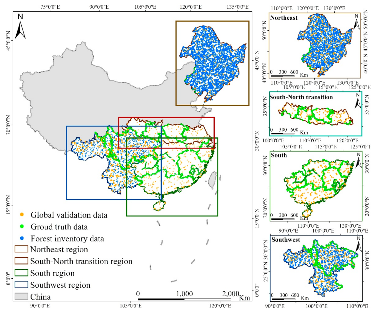
Four regions which have been identified as the main forested areas in China [15,16,17,18]—the northeast (NE), southwest (SW), south (SO), and south–north transition (SNT) regions, as shown in Figure 1—were selected for forest type classification. The NE region belongs to the mid- and high-latitude zone in China, extending between 118–135° E and 48–55° N. It straddles the temperate and cold temperate zones from S–N and has a temperate monsoon climate, with an annual precipitation in the 300–1000 mm range. NE forest areas are mostly distributed in the Daxing’an, Xiaoxing’an and Changbai Mountains and consist mainly of needle-leaved, mixed, and deciduous broad-leaved forests.
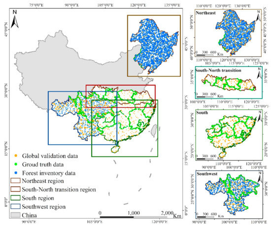
Figure 1.
Study area and reference data distribution.
The SW region is a complex mountainous area in southwest China, with a wide and balanced distribution of various geomorphic forms, and is located between 83–107° E and 21–30° N. It has a humid, subtropical monsoon climate, with an annual precipitation range of 800 mm–1600 mm. The forest areas in this region are concentrated in the Hengduan Mountains, at the junction of Sichuan, Yunnan, and Tibet, including the Yarlung Zangbo River great bend area, and the southern slope of the Himalayas in the SE Tibetan Plateau. It primarily comprises sub-alpine, needle-leaved forests.
The SO region has the highest rainfall in China, with an average annual precipitation of 6558 mm, and enjoys a tropical and subtropical monsoon climate. It is located between 102–127° E and 15–25° N. The SO forests cover a very large area to the south of the Qinling–Huaihe area and to the east of the Yunnan–Guizhou plateau, which mainly includes artificial, natural, and cash-crop forests.
The SNT zone spans the warm temperate and subtropical zones, and is the most important geological–ecological transition zone on the Chinese mainland, with a high degree of environmental complexity, biodiversity, and climate sensitivity [18]. It has mostly evergreen broad-leaved, deciduous broad-leaved, and deciduous needle-leaved forests [18,19].
2.2. Data
2.2.1. Spectral Remote Sensing Imagery
Sentinel-2 Top-of-Atmosphere (TOA) data from 2015–2019, available on the GEE cloud platform, were organized into composite, seamless, cloud-free 10 m resolution images and temporal features of red edge bands were extracted. We only took advantage of imagery obtained between the growing and deciduous seasons, which allowed us to use the monthly average normalized difference vegetation index (NDVI) for the forested regions. Cloudy pixels were masked using Sentinel-2 QA60 band [20].
Landsat Surface Reflectance (SR) data collections, with <80% cloud cover, covering the period 1985–2019, and including Landsat 5, 7, and 8 imagery available on the GEE cloud platform, were used to derive temporal features for forest type classification. Cloud cover was removed using the pixel QA band of the Landsat SR data.
2.2.2. Reference Data
Reference data included field survey data, global validation samples, and forest inventory data, which were collected in three ways:
- (1)
- field survey data: extensive field surveys in 2013, 2014, and 2018 were conducted to survey land-cover types, with 3556 ground samples collected, covering various forest types and non-forest areas;
- (2)
- global validation samples: this dataset was provided by the research team from Tsinghua University (http://data.ess.tsinghua.edu.cn/, accessed on 1 March 2020) and included 1076 data samples [21];
- (3)
- forest inventory data: these data were downloaded from the Chinese Forest Scientific Data Center (http://www.cfsdc.org/, accessed on 1 March 2020).
We randomly generated samples using ArcGIS 10.4 software and labeled the forest types using the nomenclature of the forest type inventory map. The distribution of all samples can be seen in Figure 1.
All forest type classification reference data acquired from the three sources above have been listed in Table 1. Among these, two-thirds of the training dataset were used for model training and one-third of the training dataset was used for testing to obtain the optimal feature set. The validation data were used to validate the classification map.

Table 1.
Forest classification reference data.
2.2.3. Auxiliary Data
Ancillary data included digital elevation model (DEM) data from the Shuttle Radar Topography Mission (SRTM), at a resolution of 1 arcsec (~30 m). To prepare this data, we initially applied mosaic and clip functions to SRTM data on GEE, and acquired the subset covering the study area. Then, we derived the slope and aspect features based on the resampled SRTM data, using a 10 m spatial resolution.
2.3. Methods
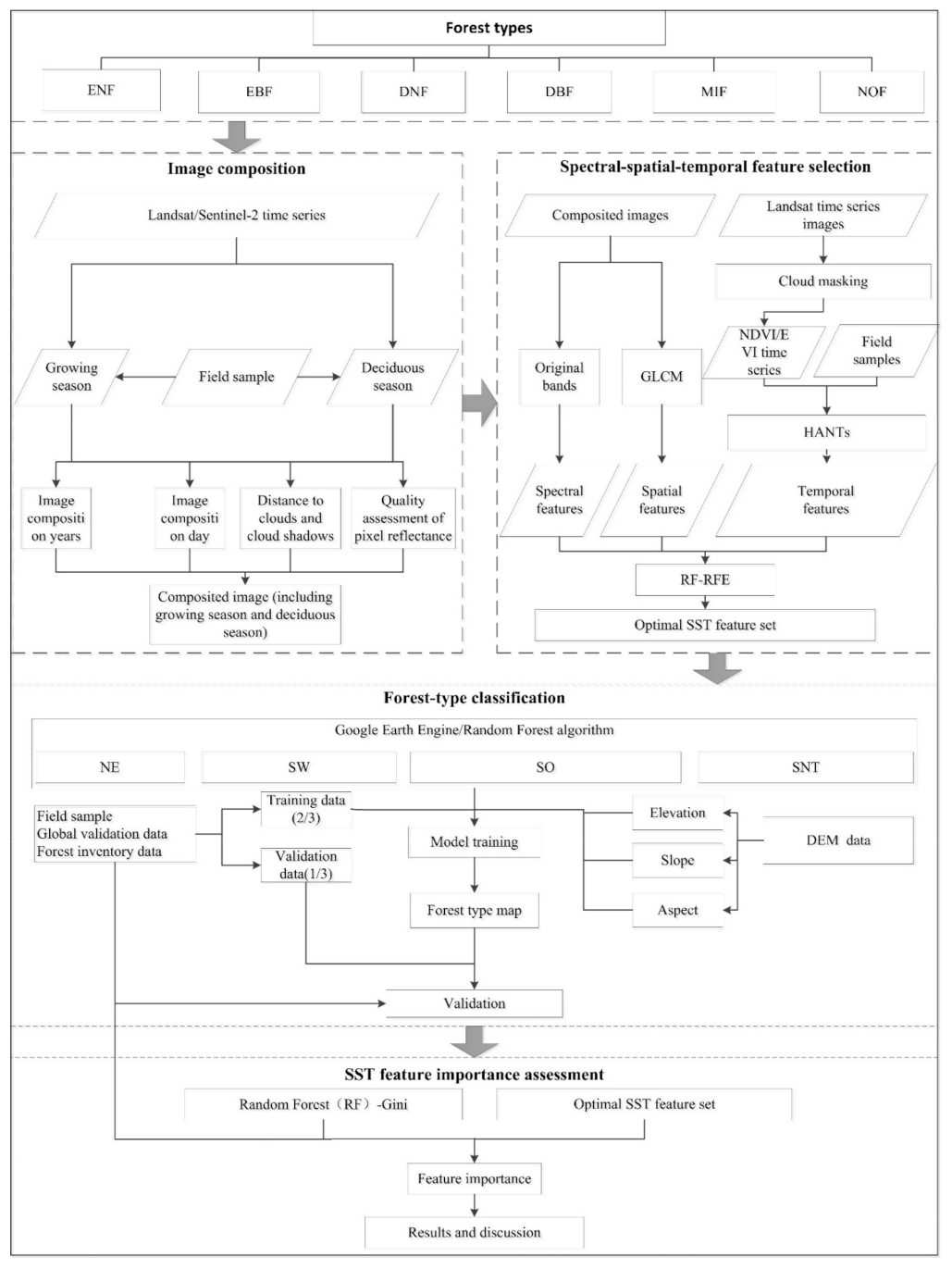
Our methodology involved the following steps (shown in Figure 2):
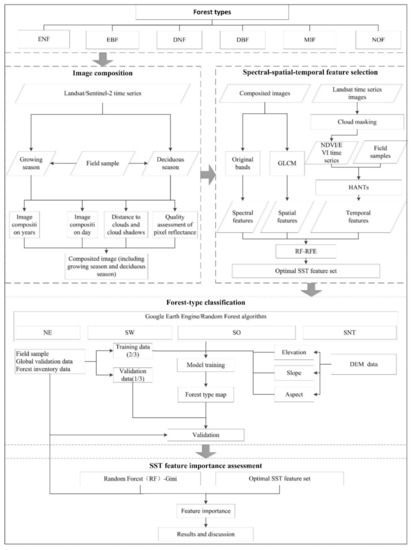
Figure 2.
Methodology workflow for mapping forest types using a 10 m resolution and based on spectral–spatial–temporal features.
- (1)
- image composition to create new images of growing and deciduous forests without cloud cover was undertaken using Sentinel-2 (TOA data for image composition) and Landsat (surface reflectance data to determine growing and deciduous season timing) time series imagery;
- (2)
- spectral–spatial–temporal feature selection was undertaken (see Section 2.3.2 for more details);
- (3)
- forest type classifications for different regions were established using the GEE platform and random forest (RF) algorithms and evaluations;
- (4)
- an SST feature-importance assessment was conducted using the Gini criterion.
2.3.1. Image Composition
- (1)
- Image composition period: the image composition period was obtained by using monthly average NDVI values for the period 1985–2019. The lengths of the growing season and deciduous season were determined by the months with an average NDVI ≥ 95% for the peak value of greenness [22,23]. This presented the period from June to October as the growing season and the months from November to April of the next year as the deciduous season in the NE forest region. For the SW forest region the growing season was from July to September and the deciduous season was between December and March of the next year. For the SO forest region the growing season was from June to October and the deciduous season was between December and April of the next year. For the SNT forest region the growing season was from June to September and the deciduous season was from December to the next year’s March. Temporal weight was calculated using a Gaussian function. The pixels whose acquisition date represented the date at which the maximum (for growing season) or minimum (deciduous season) average NDVI value was reached were assigned a value of 1 while pixels obtained at the beginning or end of the image composition period were assigned a value of 0.1.
- (2)
- Image composition years: in order to obtain high-quality remote sensing images covering the study area to the greatest extent and minimizing the impact of land class changes, the image composition years were set to three years from 2017 to 2019. Specifically, the highest weights were assigned to the pixels from 2018.
- (3)
- Distance to clouds and cloud shadows: we first masked “opaque” and “cirrus” pixels (bits 10 and 11 from the QA60 band) and then expanded these masks by 1200 m to exclude cloud edges from the images. Then, we computed a cost–distance function for the data to define the distance to clouds for all unclouded pixels and then assigned weights to the unclouded pixels based on this distance, using the sigmoid function. This s-shaped curve provided full weight to unclouded pixels, with a distance ≥ 1500 m to the clouds, and the weights then decreased, according to the sigmoid function, for pixels closer to the clouds or cloud shadows [24,25].
- (4)
- Quality assessment of pixel reflectance: NIR bands were used to perform pixel reflectance quality assessment [26]. Specifically, the median pixel-level NIR value of all image dates for the composition period was calculated to define the optimal quality of the NIR value. Pixels with an NIR value equivalent to the median NIR value were assigned the highest weight of 1, pixels with the largest absolute deviation from the median were given the lowest weight of 0, and pixels with intermediate NIR values were linearly weighted based on their absolute deviation from the median. Then, the image composition was determined by calculating the arithmetic mean of the temporal, cloud distance, and quality weights. We selected the highest mean value pixels to establish composites for each forest region [26].
2.3.2. SST Feature Selection for Forest Type Classification
- (1)
- SST Features
Four types of feature sets were derived under the SST framework, including spectral, spatial, temporal, and auxiliary features. Table 2 shows the composition of the features and the associated data sources and calculation methods. The SST framework in this study involved 114 features.

Table 2.
Descriptions of the features set in the spectral, spatial, and temporal (SST) framework.
- Spectral features were derived from composited images, which included two types. One type was the original band from the Sentinel-2 image, including seven bands from blue to NIR, which were proved efficient for vegetation identification [27], while the other was the vegetation index calculated by a combination of different bands, namely, NDVI, the normalized difference water index (NDWI), the modified soil-adjusted vegetation index (MSAVI), and the enhanced vegetation index (EVI). Three additional vegetation indices were based on derived normalized difference red-edge 1, 2, and 3 bands (NDVIre1, NDVIre2, and NDVIre3, respectively).
- Spatial features were represented by the contrast (Con), entropy (Ent), correlation (Cor), and variance (Var) of the texture features for each selected spectral feature band, based on a gray-level co-occurrence matrix (GLCM).
- Temporal features were extracted from Landsat imagery covering 1985–2019. Harmonic analysis (HANTS) was used to fit the blue, green, red, and NIR bands and the vegetation indices (NDVI and EVI). Three temporal features—including annual amplitude, phase, and root mean square error (RMSE)—were derived to describe phenological changes in different forest types. As Landsat data did not include red-edge bands, the available Sentinel-2 2015–2019 imagery was used to extract temporal features for red-edge bands.
In addition to the SST features above, auxiliary features, including elevation, slope, and aspect, were added. We implemented all of the above operations in GEE and resampled 114 features to 10 m to ensure a consistent spatial resolution.
- (2)
- Feature Selection
One hundred and fourteen features were obtained under the SST framework; however, redundant information existed among these features, causing an overfitting problem in model training. Accordingly, a random forest-recursive feature elimination (RF-RFE) algorithm was applied to execute feature selection and was implemented using Python software. Four steps were included in this process: (1) training of the RF model to obtain the importance of each feature; (2) sorting by feature importance; (3) removal of the least important feature; (4) repeat of steps 1–3 until all features have been either selected or removed [19].
2.3.3. Classification, Accuracy, and Feature Importance Assessments
Based on the optimal SST feature set, the RF algorithm on GEE was used to classify forest types for each region, building ensembles of 100 trees, while the other RF parameters were set to default values. The confusion matrix was calculated to evaluate the classification results, using the independently validated samples (Table 1). The overall accuracy (OA), producer’s accuracy (PA), and user’s accuracy (UA) were derived through the confusion matrix and were used to perform accuracy assessments.
Feature importance assessment was used to determine which SST features contributed more to the classification of various forest types in each region. This was performed using the Gini criterion in the RF algorithm, which could quantify feature contributions (as a value in the range zero to one). For the five forest types (EBF, DBF, ENF, DNF, and MIF), a total of 11 evaluation scenarios were designed to determine the importance of SST features in each paired forest type classification. They consisted of EBF paired with DBF (EBF vs. DBF), EBF paired with ENF (EBF vs. ENF), EBF paired with DNF (EBF vs. DNF), EBF paired with MIF (EBF vs. MIF), DBF paired with ENF (DBF vs. ENF), DBF paired with DNF (DBF vs. DNF), DBF paired with MIF (DBF vs. MIF), ENF paired with DNF (ENF vs. DNF), ENF paired with MIF (ENF vs. MIF), DNF paired with MIF (DNF vs. MIF), and all five forest types (for reference). In terms of each scenario, a single RF classifier was applied for training, using the data from only the specified types—for example, training for the EBF vs. DBF feature importance assessment was performed only on pixels from EBF and DBF samples.
3. Results
3.1. SST Features
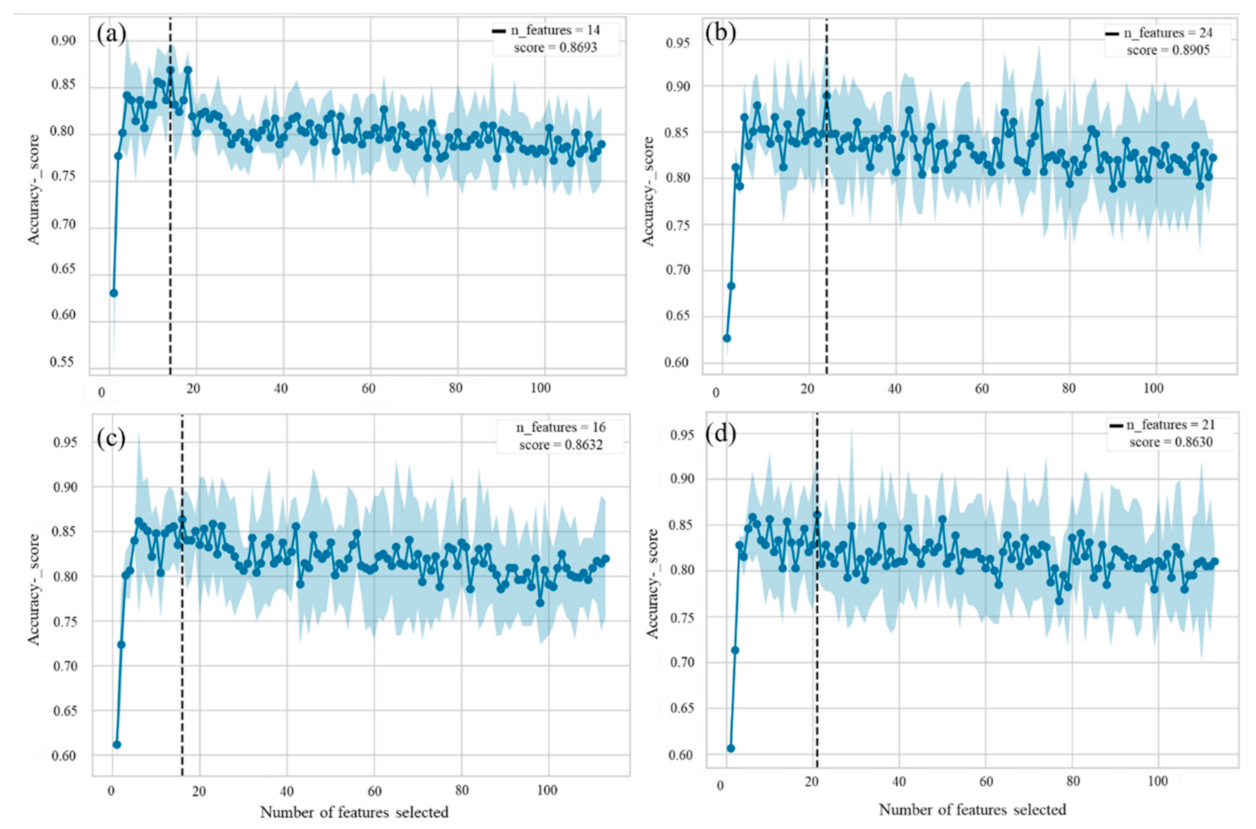
The optimal number of SST features for different regions was obtained by executing RF-RFE 20 times [19,27], as shown in Figure 3 and Table 3.
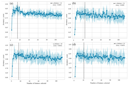
Figure 3.
Optimal numbers of features and SST feature lists for the (a) northeast (NE); (b) southwest (SW); (c) south (SO); and (d) south–north transition (SNT) regions.

Table 3.
Optimal SST feature list for the four studied regions.
NE (Figure 3a): the highest accuracy (0.8693) occurred when the number of features was 14, and as the number of features increased beyond this, classification accuracy dropped. Closer examination revealed that in this region (Table 3), the spectral features mainly included redE1, NDVIre1, and NDVIre2 for the growing season, and redE2, NDVIre2, and EVI for the deciduous season. Only three spatial features remained, namely, red_con and redE1_ent from the growing season and nir_var from the deciduous season. The temporal features remaining were NDVI_amp, NDVI_rmse, EVI_pha, and redE2_rmse, with the elevation indicator derived from the DEM also retained.
SW (Figure 3b): the best accuracy (0.8905) occurred when the number of features reached 24, and it showed a similar trend to NE, although with different remaining features (Table 3). Among all the features, the number of spectral features was apparently more than that of the other feature types and included the blue, redE1, and NIR bands, and the NDVIre1, NDVI, and EVI indices, from the growing season, along with the green, redE3, and NIR bands, and the NDVIre3 and EVI indices, from the deciduous season. The spatial features remaining were derived from the red, nir, and redE1 bands and included red_con, red_cor, and nir_ent, derived from the growing season, and redE1_var and nir_con from the deciduous season. Temporal features in the SW for forest type classification included redE1_rmse, redE2_rmse, NDVI_amp, NDVI_rmse, EVI_pha, and NDVI_pha and, except for elevation, the auxiliary features were also retained for this aspect.
SO (Figure 3c): the best-fit number for forest type classification in the SO was 16, with an accuracy of 0.8632. In the determined feature list (Table 3), spectral features included the blue and redE1 bands, together with the NDVIre1 and NDVIre2 indices for the growing season, along with the blue and redE3 bands and the NDVIre3 index from the deciduous season. The number of spatial features remained the smallest among the SST features, with only three—nir_con and nir_cor from the growing season and red_var from the deciduous season. The temporal features remaining in this region were redE1_amp, redE1_pha, NDVI_pha, and EVI_pha, while for the auxiliary features, elevation and slope remained, affecting the forest type classification.
SNT (Figure 3d): the peak classification accuracy (0.8630) corresponded to a feature quantity of 21. The detailed feature list indicated that spectral features constituted the largest number, including green, red, nir, NDVI, and EVI for the growing season and blue, green, red, nir, and NDVI for the deciduous season (Table 3). The only spatial features retained were nir_con and red_con from the growing season and nir_con and red_cor from the deciduous season. The temporal features were all derived from EVI and NDVI indices and included EVI_pha, NDVI_pha, EVI_amp, NDVI_amp, EVI_rmse, and NDVI_rmse, while only elevation remained in the auxiliary feature set.
3.2. Forest Cover Map
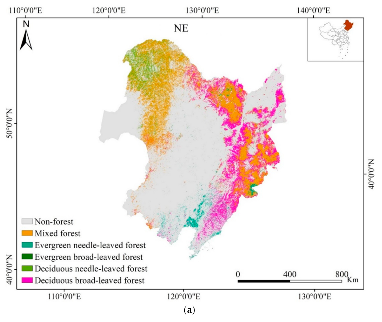
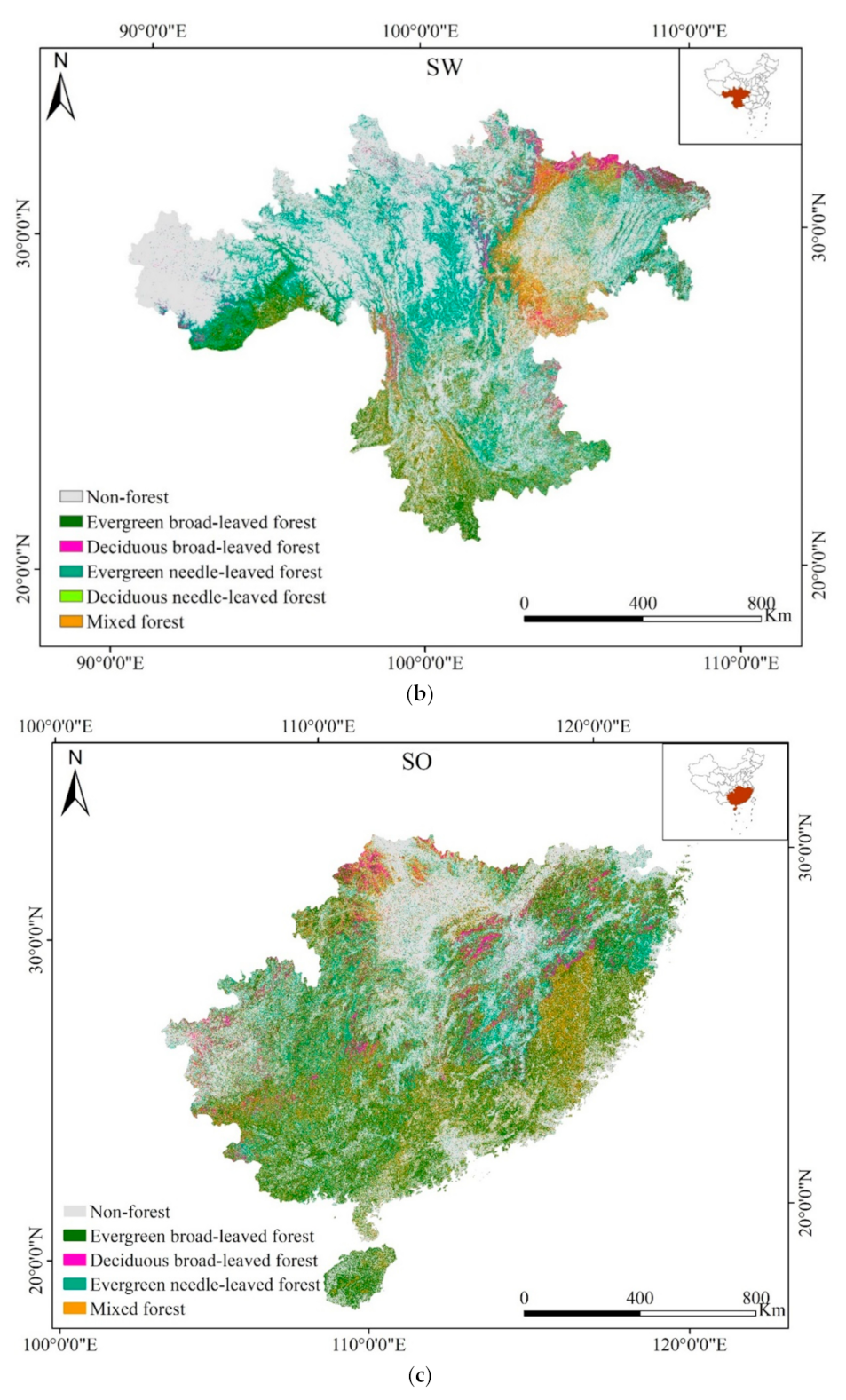
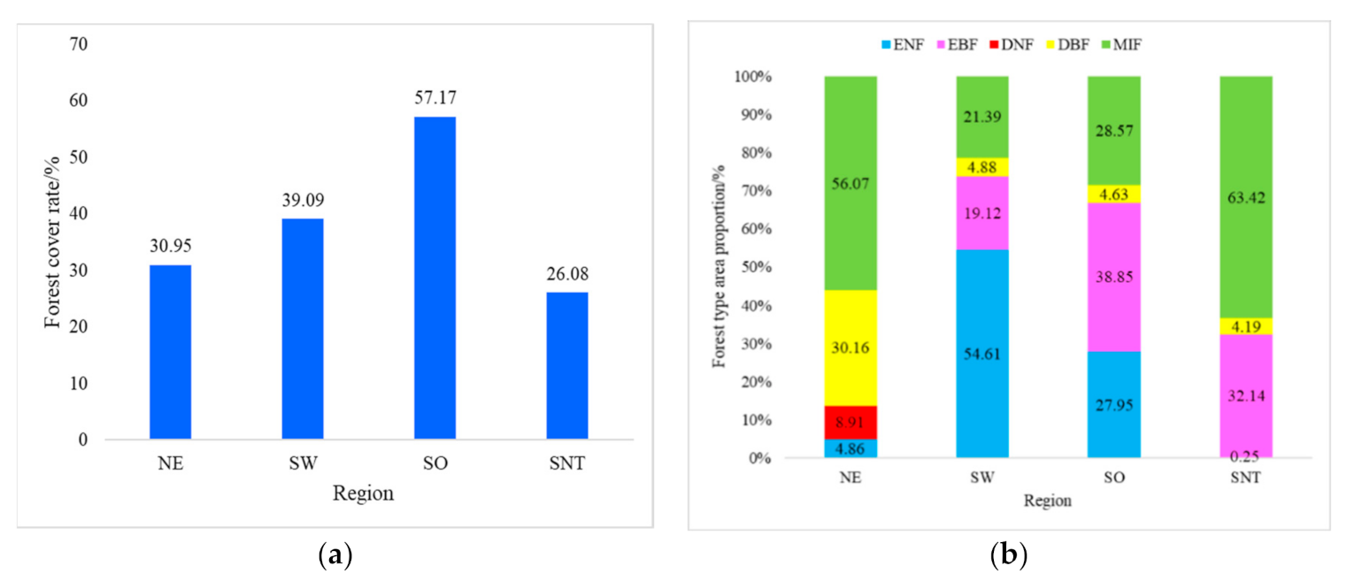
The classification results are shown in Figure 4. The forest cover rate and areal proportion for each forest type were calculated and are presented in Figure 5.

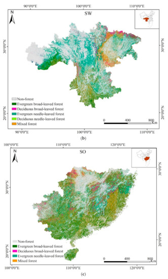
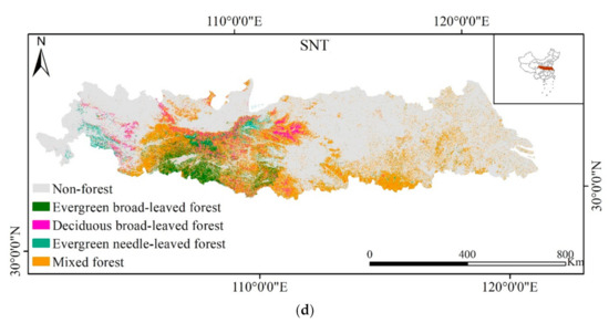
Figure 4.
Regional forest type coverage (10 m resolution) in 2018 for the (a) NE; (b) SW; (c) SO; and (d) SNT regions.

Figure 5.
Forest cover rate (a) and regional proportions of each forest type (b).
NE (Figure 4a): forest types mainly included MIF, DBF, and DNF, which were mostly distributed around the Daxing’an and Xiaoxing’an Mountains and around Changbai Mountain. It was apparent that the proportion of DNF in NE China was significantly higher than in the other three regions examined, and was distributed in the east and north of the Daxing’an Mountains. This was consistent with the fact that NE China is the largest DNF-producing area nationally [28]. It could also be seen that forest resources in NE were mainly concentrated in the border areas (adjacent to Russia, North Korea, and Mongolia), which included more forests than other areas. The forest coverage rate in NE was approximately 30.95%, with MIF contributing 56.07% of this, followed by DBF (~30.16%). The results showed that ENF contributed the least, accounting for just 4.86%.
SW (Figure 4b): the forest types in the SW region included ENF, EBF, DNF, DBF, and MIF. ENF and EBF were found distributed around the Hengduan Mountains, in the center, west, and south of the SW region. The amounts of MIF and DNF were relatively small, and were concentrated in the eastern part of the region, while the DBF was located mainly in the south-central region. Forest coverage rate in the SW was found to be approximately 39.09%, with ENF representing the largest portion, accounting for 54.62%. MIF and EBF followed, with 21.39% and 19.12%, respectively, with DBF having the smallest coverage, at approximately 4.88%.
SO (Figure 4c): EBF, ENF, MIF, DBF, and DNF forest types were seen to occur in SO, and were mostly concentrated in the southern and eastern areas of the region, with a forest-cover rate of 57.17%. The amount of EBF accounted for 38.85% of the forest area, followed by MIF and ENF (28.57% and 27.95%, respectively), with DBF covering the smallest area, at 4.63%.
SNT (Figure 4d): the forest resources here were found to be mainly distributed near the Qinling Mountains, in the central and western areas of this region. The forest types were mainly MIF, EBF, and DBF, and were concentrated in mountainous areas at higher elevations, such as Taibai Mountain of the Qinling Mountains area. The forest coverage rate in this zone was approximately 26.08%, with MIF accounting for 63.42% of the total, followed by EBF, at 32.14%, and then DBF and ENF, which covered 4.19% and 0.25% of the area, respectively.
3.3. Accuracy Assessment
In the NE area, 715 field validation samples were used to assess result accuracy and the OA was found to be 91.47% (Table 4). Among all the forest types, DBF had the highest PA and UA (98.89% and 100%, respectively), which suggested that almost all DBFs in this region had been mapped accurately.

Table 4.
Accuracy assessment confusion matrix for the NE forest type map.
In the SW, 616 field validation samples were employed to assess the accuracy, giving an OA of 86.85%, as shown in Table 5. Here, EBF acquired relatively high PA (97.44%) and UA (82.61%) results, which suggested that this forest type had been classified with fewer omission and commission errors than the others, and that EBF coverage had been provided at a relatively high accuracy level in this region.

Table 5.
Accuracy assessment confusion matrix for the SW forest type map.
In the SO, 815 field validation samples were used to evaluate classification accuracy, and the confusion matrix (Table 6) showed that the regional OA was 93.50%. The most accurate classification result here was obtained for EBF, with both PA and UA > 90%.

Table 6.
Accuracy assessment confusion matrix for the SO forest type map.
For the SNT, 302 field validation samples were obtained and, as shown in Table 7, the OA here was found to be 92.38%. ENF achieved PA and UA values of >90%, showing that the ENF area in the SNT region had been provided with a relatively high level of accuracy.

Table 7.
Accuracy assessment confusion matrix for the SNT forest type map.
3.4. Feature Importance Assessment
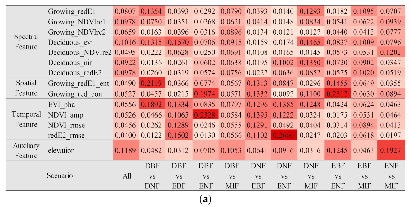
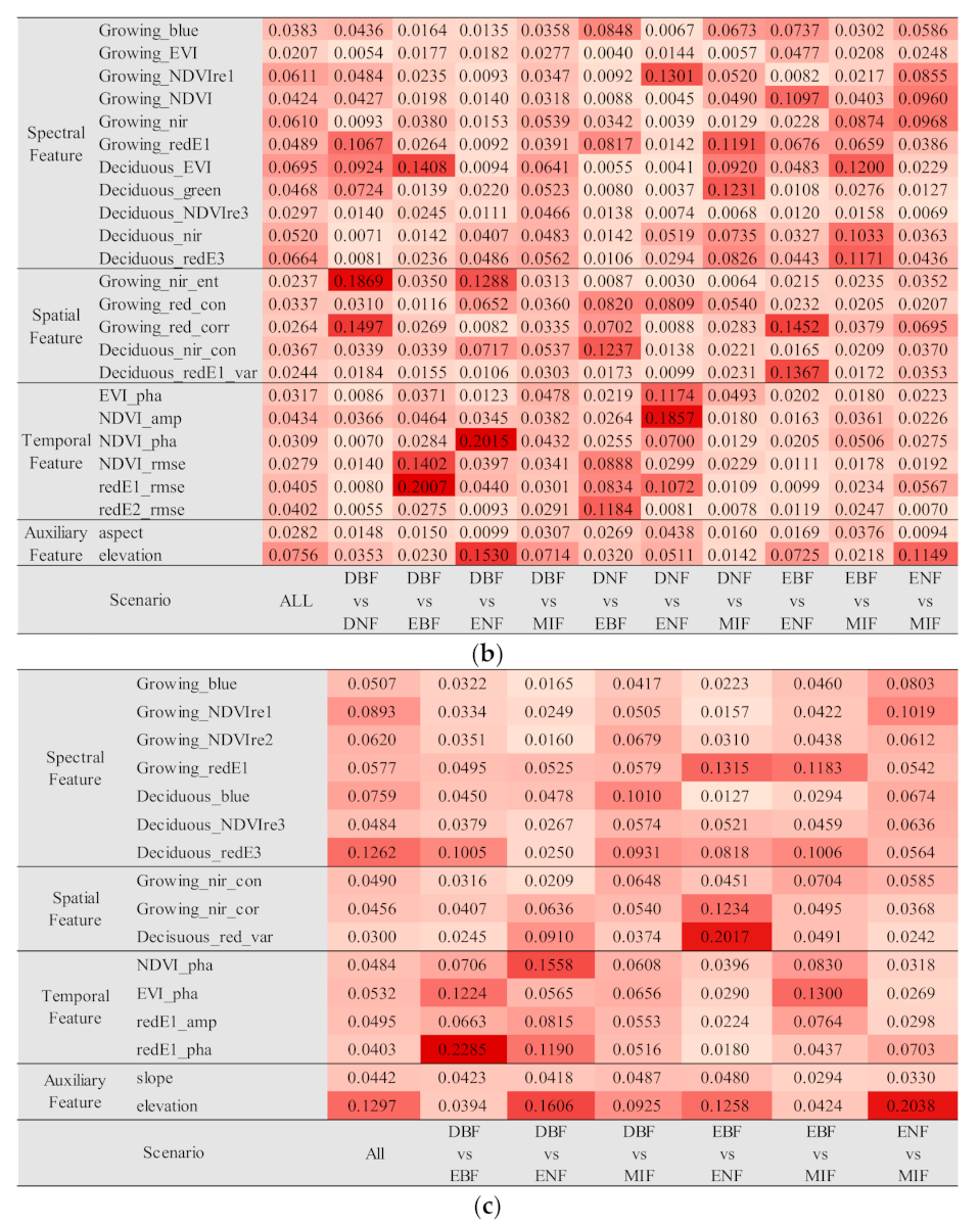
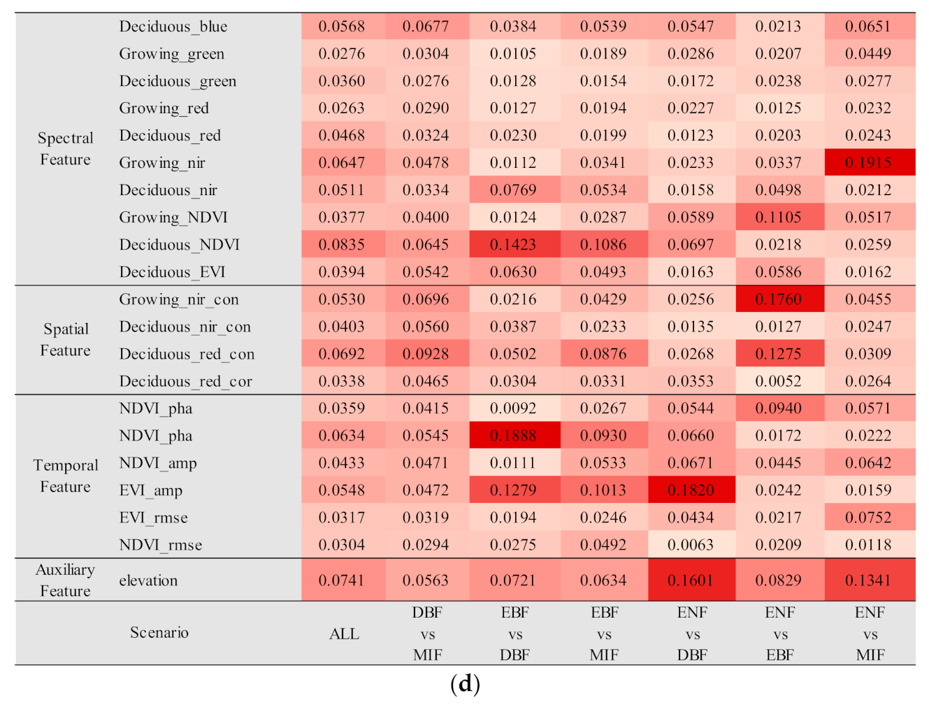
Feature importance represented differences in contribution when classifying various forest types in the four regions (Figure 6). Overall, when the classifier was trained on all forest types, it was found that the importance of the SST features was analogous and that the performance of each feature was relatively average, with no apparent mutation. However, when discriminating between any two forest types, the contributions from the features represented significant differences.

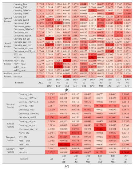
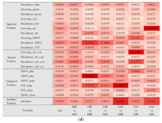
Figure 6.
Feature importance in forest type classifications for the (a) NE; (b) SW; (c) SO; and (d) SNT regions.
NE: temporal features played a vital role in discriminating between evergreen and deciduous forests, which were the main forest types in this region and were significantly seasonal. Spectral features contributed more to the classification of mixed forests with complex forest types, whereas spatial features played a more significant role in the classification of needle-leaved and broad-leaved forests.
SW: spectral and temporal characteristics were relatively more important in this region, with spatial characteristics being slightly less for all forest type divisions. Temporal features played a significant role in the classification of evergreen and deciduous forests, while spectral features were better suited to classifying all forest types and mixed forests. In addition, the auxiliary features of this region also made contributions, particularly with respect to the complex regional topography, as exemplified by Hengduan Mountain.
SO: the prominent feature here was the elevation featureof auxiliary features, which played a significant role in classifying all forest types and specific forest types, indicating that forest type distribution here was largely correlated with elevation. Temporal features played a greater role in the classification of evergreen and deciduous forests, while spectral features were generally more uniform, maintaining a stable role in identifying forest types. The contribution made by spatial features was insignificant compared with that made by other feature types.
SNT: spectral features contributed the most to forest type classifications here, accounting for the largest percentage in most assessment results and having the greatest significance in classifying evergreen and deciduous forests. This was followed by temporal features, particularly in the classification of evergreen and deciduous forests; spectral features had the greatest significance, with spatial features playing a lesser role, affecting only ENF and EBF classification. Auxiliary features were significant in the SNT region, which indicated that the forest types here were greatly affected by elevation—as was expected, given the significant vertical distribution of vegetation types in this area.
4. Discussion
4.1. Image Composition Method
Obtaining high quality and reliable composite images is an important prerequisite for studying the SST feature set and its application in the use of remote sensing data in forest classifications. In this study, we adopted a method for pixel-based, multi-rule compositing of Sentinel-2 archive data to generate cloud-free images for the four studied regions. The adopted image composition method made full use of pixels over the same period for many years and assigned weights according to set rules, making the composition results more reliable. The image composition method presented is flexible and the rules can be adjusted for different information needs.
Four parameters—image composition years, image composition period, distance to clouds and cloud shadows, and quality assessment of pixel reflectance—were used to obtain synthetic images of the growing and deciduous seasons in the four different regions [25,26,29]. The image composition years were set to three in this study, allowing composite images covering the growing and deciduous seasons to be obtained for the four regions. The image composition period was determined using those months with an average NDVI ≥ 95% of the peak greenness value [22,23,26], and the resulting periods for the four regions can be seen in Table 8. Distances to clouds/cloud shadows were calculated to determine the suitability of each pixel for the composition. The assessment of the pixel reflectance was performed to avoid oversaturation, clouds, or shadowed pixels that were omitted in the cloud masking. These pixels were included in the NIR image composite, as it showed the least noise over forested areas [22].

Table 8.
The image composition periods for growing and deciduous seasons.
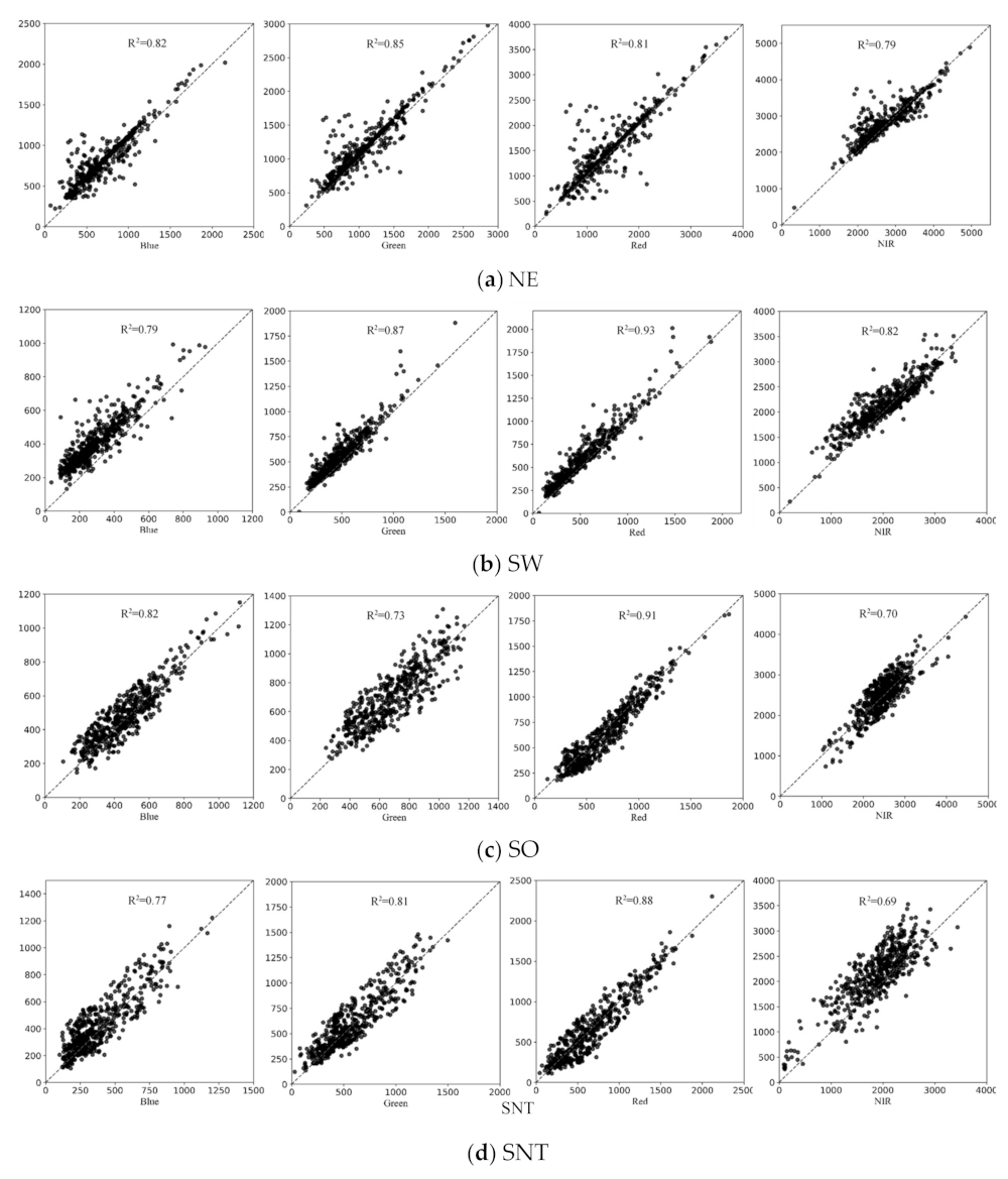
Furthermore, in order to assess the composition results, 500 sample points were randomly selected from a single image, withholding the most cloud-free pixels as a reference, to evaluate the consistency of the synthesis results for the four regions on GEE. The assessment result was as shown in Figure 7. The surface reflectance values in the composite image for the four regions exhibited strong correspondence with the reference images in the blue, green, red, and NIR bands, with R2 values ranging from 0.69–0.93.
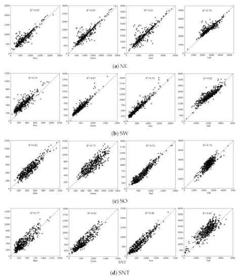
Figure 7.
Quality assessments for NE, SW, SO, and SNT composite images; surface reflectance values from a reference image are plotted against composite surface reflectance values (reflectance values are scaled by 10,000).
4.2. SST Forest Types Classification Framework
Forests can grow in many different climates, from the tropics to cold temperate zones, and forest compositions and types are diverse—which poses many challenges when using remote sensing technology for large-scale forest mapping. In previous studies, single classification methods and coarse resolution remote sensing images were used for forest classification and mapping on a large scale, often ignoring differences in forest distribution in different climate zones [21].
The SST forest type classification framework applied here comprehensively took account of the distribution characteristics of forests in different climates or latitudes, and registered differences between forest types from spectral, spatial, and temporal perspectives. This was the first study to make full use of the characteristics available in Landsat and Sentinel-2 time series data for application in forest classification, and we collected as much spectral, spatial, and temporal feature data as possible from them. The results showed the SST classification framework to be effective for mapping large-scale forest areas, especially across climate zones.
With regard to spectral features, we considered the fact that Sentinel-2 data include more spectral information than Landsat data and used the Sentinel-2 spectral feature set with the original bands and vegetation indices. Previous studies have shown that these features are all suitable for forest classification [6,7,19]. Considering the unique red-edge bands in Sentinel-2, we replaced the NIR band with the red-edge band, based on the theoretical NDVI, acquiring three red-edge indices (NDVIre1, NDVIre2, and NDVIre3). The evaluation results for feature importance also showed that various types of features related to the red-edge bands showed greater significance, indicating that the red-edge bands could make a relatively important contribution to forest type classifications.
Spatial features were derived from Sentinel-2 images composited using their high spatial resolution and were described using the texture index calculated using the GLCM method. We adopted this approach as the texture features could show basic attributes (size, density, and reflectance) of internal canopy shadows and leaves [30]. We selected the contrast (con), entropy (ent), correlation (cor), and variance (var) of the texture features for each selected band to represent spatial features, these having been previously shown to be effective in discriminating forest types [19,27,31,32,33].
Temporal features were extracted using the HANTS method, using the long NDVI and EVI time series derived from Landsat time series data. NDVI and EVI time series have been shown to reflect forest growth indicators and have been widely used in temporal feature extraction [19,34,35,36].
4.3. Feature Importance for Forest Type Classification
In the feature importance assessment, the indices ranked highly were mostly from the temporal feature set, suggesting that the time series indices were generally more helpful for forest type classification—which is consistent with the findings of Pasquarella [6]. Furthermore, our study found that in areas with different geographic characteristics, the features which were most important for forest type classification varied. In the middle- and high-altitude areas of NE China, the indicators in the temporal feature set played a significant role. For complex mountainous areas in SW China, the importance of spectral feature indicators increased, being significantly higher than that in other areas. In terms of cloudy and rainy southern regions, spectral and temporal features played a similar role, while spatial features clearly played a larger role in SW China than in the other studied regions. For the climate transition zone in China, elevation, from the auxiliary features set, played a relatively important role in classifying each forest type. We also saw that the role of time features was most important here, especially for separating evergreen and deciduous forests.
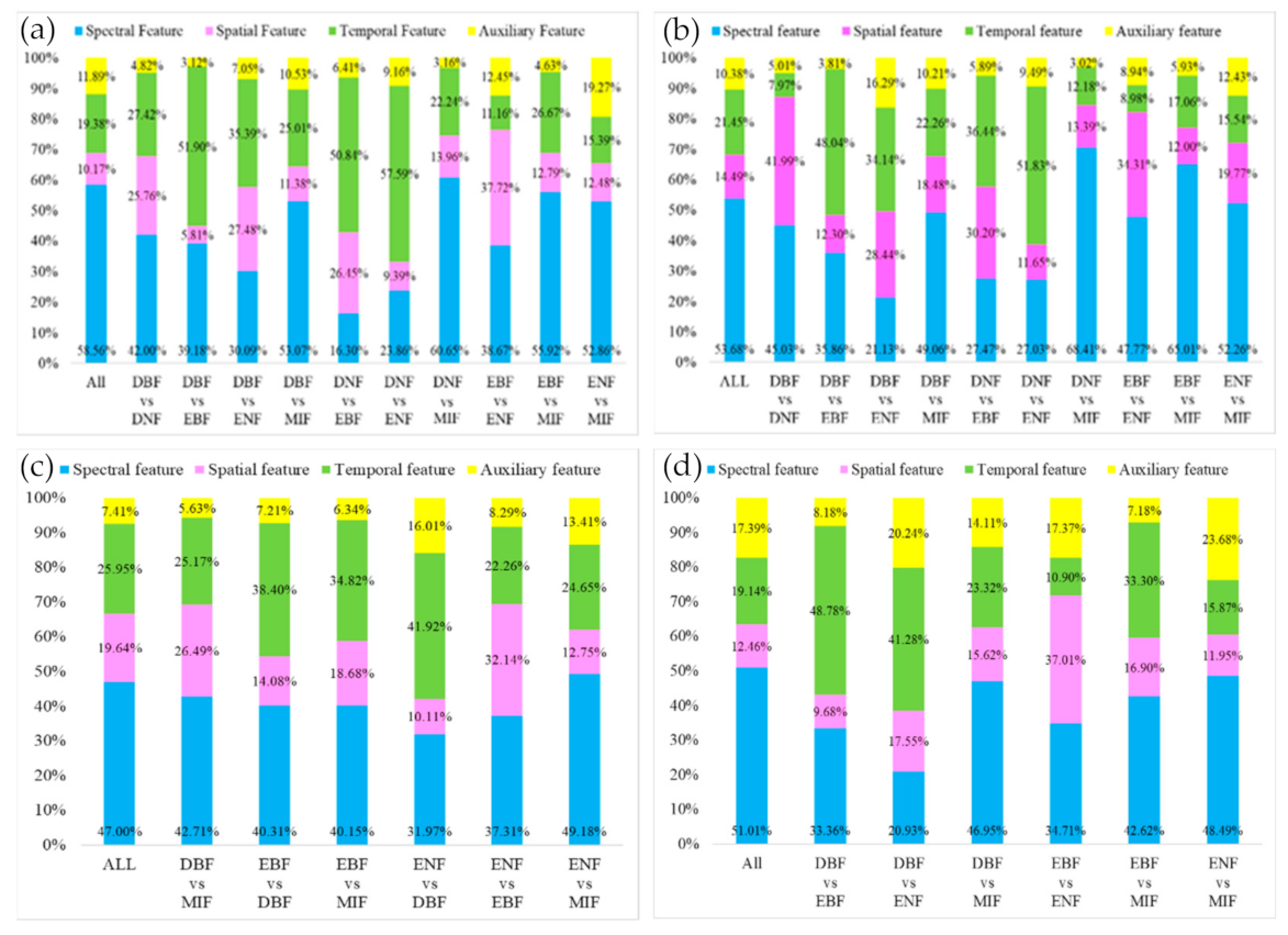
In terms of the general feature importance, spectral feature importance accounted for the majority of the ratio (Figure 8) in the four regions, suggesting that spectral features derived from remote sensing images remained the most important in forest type classification processes. We saw that spectral features performed particularly well in classifying complex forest types, such as MIF. The importance of temporal features was second only to spectral features in most scenarios (Figure 8), being particularly evident with regard to the classification of evergreen and deciduous forest types with significant differences in growth patterns, where temporal features were found to have major significance.

Figure 8.
Importance of individual features from the SST feature set in the (a) NE; (b) SW; (c) SO; and (d) SNT regions.
Although some features in the spatial features set had higher values—for example, in classifying DBF and DNF in the SW region, the spatial features Growing_nir_ent and Growing_red_cor presented the greatest significance among all the features—the overall effect produced by spatial features was the smallest among the SST features in most schemes, which may be related to their limited number. For some forest types with distinct spatial structural differences, however, such as needle-leaved and broad-leaved forests, spatial features produced optimal effects (Figure 8b). We found that topography was one of the major factors influencing forest type classification, especially in mountainous areas and areas with large elevation transitions, with forest type often affected by terrain elevation, slope, and aspect, as has been previously reported [19].
Overall, for forest type classification, although a single feature sometimes played a significant role (e.g., NDVI amplitude in the temporal feature set), the optimal result was often obtained through a combination of SST features. Hence, the power of SST features in our work depended on the combination of features which characterized SST variability in reflectance properties. This was illustrated by the results of the feature importance assessment and suggested that SST features all played significant roles in the forest type classification process.
5. Conclusions
In this study, we conducted a detailed classification of forest types, using characteristics available from multi-source time series remote sensing sources, particularly high spatial resolution image data for large areas. Based on the GEE cloud computing platform and machine learning algorithms, we established an extraction framework for the SST features of forest type classification. Considering four typical Chinese geographic regions (middle and high latitudes, complex mountainous areas, cloudy and rainy areas, and the SNT zone) as examples, the accuracy of the method was verified and a forest type map for 2018 was obtained with a 10 m spatial resolution. The results achieved an overall classification accuracy of > 85%, which indicated that the proposed method was reliable.
The feature indicators that affected the forest type classifications differed with geographical location. We found that when classifying each forest type, spectral features were more important in classifications involving complex compositions, with our feature importance assessment demonstrating that red-edge bands were very useful in forest type classification. Temporal features could be very important in identifying forest types with distinct evergreen and deciduous growth patterns, while spatial features produced better classification results for forest types with different spatial structures, such as needle- and broad-leaved forests. We also saw that topographic factors were indispensable indicators for classifying forest types in mountainous areas or areas with large elevation transitions.
Author Contributions
Conceptualization, Methodology, Investigation, Resources, K.C. and J.W.; Software, Validation, Data curation, Writing—original draft preparation, K.C.; Writing—review and editing, J.W., X.Y. All authors have read and agreed to the published version of the manuscript.
Funding
This research was funded by the Strategic Priority Research Program (class A) of the Chinese Academy of Sciences, grant number XDA19040501; the 13th Five-Year Informatization Plan of the Chinese Academy of Sciences, grant number XXH13505-07; and the Construction Project of the China Knowledge Center for Engineering Sciences and Technology, grant number CKCEST-2020-2-4.
Informed Consent Statement
Informed consent was obtained from all subjects involved in the study.
Data Availability Statement
Not applicable.
Conflicts of Interest
The authors declare no conflict of interest.
References
- Food and Agriculture Organization of the United Nations. The State of the World’s Forests 2018—Forest Pathways to Sustainable Development; Food and Agriculture Organization of the United Nations: Rome, Italy, 2018. [Google Scholar]
- UNSC. Revised List of Global Sustainable Development Goal Indicators, United Nations Statistical; UNSC: New York, NY, USA, 2015. [Google Scholar]
- Rogan, J.; Chen, D.M. Remote sensing technology for mapping and monitoring land-cover and land-use change. Prog. Plan. 2004, 61, 301–325. [Google Scholar] [CrossRef]
- Liu, Y.; Gong, W.; Hu, X.; Gong, J. Forest Type Identification with Random Forest Using Sentinel-1A, Sentinel-2A, Multi-Temporal Landsat-8 and DEM Data. Remote Sens. 2018, 10, 946. [Google Scholar] [CrossRef]
- Zhang, X.; Liu, L.; Zhang, Y.; Zhang, J.; Nie, Y.; Zhang, H. Extraction of Shrub Vegetation by Object-Oriented Classification Method Based on ENVI ZOOM in High-Altitude Area: A Case of Dingri County. Geogr. Geo-Inf. Sci. 2010, 26, 104–108. [Google Scholar]
- Pasquarella, V.J.; Holden, C.E.; Woodcock, C.E. Improved mapping of forest type using spectral-temporal Landsat features. Remote Sens. Environ. 2018, 210, 193–207. [Google Scholar] [CrossRef]
- Grabska, E.; Hostert, P.; Pflugmacher, D.; Ostapowicz, K. Forest Stand Species Mapping Using the Sentinel-2 Time Series. Remote Sens. 2019, 11, 1197. [Google Scholar] [CrossRef]
- Cheng, K.; Wang, J. Forest-Type Classification Using Time-Weighted Dynamic Time Warping Analysis in Mountain Areas: A Case Study in Southern China. Forest 2019, 10, 1040. [Google Scholar] [CrossRef]
- Zhu, X.; Chen, J.; Gao, F.; Chen, X.; Masek, J.G. An enhanced spatial and temporal adaptive reflectance fusion model for complex heterogeneous regions. Remote Sens. Environ. 2010, 114, 2610–2623. [Google Scholar] [CrossRef]
- Tamiminia, H.; Salehi, B.; Mahdianpari, M.; Quackenbush, L.; Adeli, S.; Brisco, B. Google Earth Engine for geo-big data applications: A meta-analysis and systematic review. ISPRS J. Photogramm. Remote Sens. 2020, 164, 152–170. [Google Scholar] [CrossRef]
- Gorelick, N.; Hancher, M.; Dixon, M.; Ilyushchenko, S.; Thau, D.; Moore, R. Google Earth Engine: Planetary-scale geospatial analysis for everyone. Remote Sens. Environ. 2017, 202, 18–27. [Google Scholar] [CrossRef]
- Hansen, M.C.; Potapov, P.V.; Moore, R.; Hancher, M.; Turubanova, S.A.; Tyukavina, A.; Thau, D.; Stehman, S.V.; Goetz, S.J.; Loveland, T.R.; et al. High-Resolution Global Maps of 21st-Century Forest Cover Change. Science 2013, 342, 850–853. [Google Scholar] [CrossRef]
- Shimada, M.; Itoh, T.; Motooka, T.; Watanabe, M.; Shiraishi, T.; Thapa, R.; Lucas, R. New global forest/non-forest maps from ALOS PALSAR data (2007–2010). Remote Sens. Environ. 2014, 155, 13–31. [Google Scholar] [CrossRef]
- Dong, J.; Xiao, X.; Menarguez, M.A.; Zhang, G.; Qin, Y.; Thau, D.; Biradar, C.; Moore, B., III. Mapping paddy rice planting area in northeastern Asia with Landsat 8 images, phenology-based algorithm and Google Earth Engine. Remote Sens. Environ. 2016, 185, 142–154. [Google Scholar] [CrossRef]
- Ge, Q.; Zhao, M.; Zhang, X.; Zheng, J.; Sun, H.; Zhang, P. Statistical analysis about the changes of forest resource and precipitation in China over the past 50 years. J. Nat. Resour. 2001, 16, 413–419. [Google Scholar]
- Li, M.; Zhu, Z.; Lu, H.; Xu, D.; Liu, A.; Peng, S. Assessment of forest geospatial patterns over the three giant forest areas of China. J. For. Res. 2008, 19, 25–31. [Google Scholar] [CrossRef]
- Shen, W.; Xu, T.; Li, M. Spatio-temporal changes in forest fragmentation, disturbance patterns over the three giant forested regions of China. J. Nanjing For. Univ. Nat. Sci. Ed. 2013, 37, 75–79. [Google Scholar]
- Zhang, B. Ten major scientific issues concerning the study of China’s north-south transitional zone. Prog. Geogr. 2019, 38, 305–311. [Google Scholar]
- Cheng, K.; Wang, J. Forest Type Classification Based on Integrated Spectral-Spatial-Temporal Features and Random Forest Algorithm-A Case Study in the Qinling Mountains. Forests 2019, 10, 559. [Google Scholar] [CrossRef]
- Traganos, D.; Aggarwal, B.; Poursanidis, D.; Topouzelis, K.; Chrysoulakis, N.; Reinartz, P. Towards Global-Scale Seagrass Mapping and Monitoring Using Sentinel-2 on Google Earth Engine: The Case Study of the Aegean and Ionian Seas. Remote Sens. 2018, 10, 1227. [Google Scholar] [CrossRef]
- Li, C.; Wang, J.; Hu, L.; Yu, L.; Clinton, N.; Huang, H.; Yang, J.; Gong, P. A Circa 2010 Thirty Meter Resolution Forest Map for China. Remote Sens. 2014, 6, 5325–5343. [Google Scholar] [CrossRef]
- Potapov, P.; Turubanova, S.; Hansen, M.C. Regional-scale boreal forest cover and change mapping using Landsat data composites for European Russia. Remote Sens. Environ. 2011, 115, 548–561. [Google Scholar] [CrossRef]
- Zhou, L.M.; Tucker, C.J.; Kaufmann, R.K.; Slayback, D.; Shabanov, N.V.; Myneni, R.B. Variations in northern vegetation activity inferred from satellite data of vegetation index during 1981 to 1999. J. Geophys. Res. Atmos. 2001, 106, 20069–20083. [Google Scholar] [CrossRef]
- Griffiths, P.; Kuemmerle, T.; Baumann, M.; Radeloff, V.C.; Abrudan, I.V.; Lieskovsky, J.; Munteanu, C.; Ostapowicz, K.; Hostert, P. Forest disturbances, forest recovery, and changes in forest types across the Carpathian ecoregion from 1985 to 2010 based on Landsat image composites. Remote Sens. Environ. 2014, 151, 72–88. [Google Scholar] [CrossRef]
- Griffiths, P.; van der Linden, S.; Kuemmerle, T.; Hostert, P. Pixel-Based Landsat Compositing Algorithm for Large Area Land Cover Mapping. IEEE J. Sel. Top. Appl. Earth Obs. Remote Sens. 2013, 6, 2088–2101. [Google Scholar] [CrossRef]
- Hurni, K.; Van Den Hoek, J.; Fox, J. Assessing the spatial, spectral, and temporal consistency of topographically corrected Landsat time series composites across the mountainous forests of Nepal. Remote Sens. Environ. 2019, 231, 111225. [Google Scholar] [CrossRef]
- Wang, D.; Wan, B.; Qiu, P.; Su, Y.; Guo, Q.; Wang, R.; Sun, F.; Wu, X. Evaluating the Performance of Sentinel-2, Landsat 8 and Pleiades-1 in Mapping Mangrove Extent and Species. Remote Sens. 2018, 10, 1468. [Google Scholar] [CrossRef]
- Fu, M. Nitrogen Transform and Release in Typical Temperate Forest Ecosystems in Northeastern China; Northeast Forestry University: Yangling, China, 2009. [Google Scholar]
- White, J.C.; Wulder, M.A.; Hobart, G.W.; Luther, J.E.; Hermosilla, T.; Griffiths, P.; Coops, N.C.; Hall, R.J.; Hostert, P.; Dyk, A.; et al. Pixel-Based Image Compositing for Large-Area Dense Time Series Applications and Science. Can. J. Remote Sens. 2014, 40, 192–212. [Google Scholar] [CrossRef]
- Sayn-Wittgenstein, L. Recognition of Tree Species on Aerial Photographs. Information Report FMR-X-118; Forest Management Institute: Ottawa, MO, USA, 1978. [Google Scholar]
- Wang, T.; Zhang, H.; Lin, H.; Fang, C. Textural-Spectral Feature-Based Species Classification of Mangroves in Mai Po Nature Reserve from Worldview-3 Imagery. Remote Sens. 2016, 8, 24. [Google Scholar] [CrossRef]
- Huang, X.; Liu, X.; Zhang, L. A Multichannel Gray Level Co-Occurrence Matrix for Multi/Hyperspectral Image Texture Representation. Remote Sens. 2014, 6, 8424–8445. [Google Scholar] [CrossRef]
- Ouma, Y.O.; Tetuko, J.; Tateishi, R. Analysis of co-occurrence and discrete wavelet transform textures for differentiation of forest and non-forest vegetation in very-high-resolution optical-sensor imagery. Int. J. Remote Sens. 2008, 29, 3417–3456. [Google Scholar] [CrossRef]
- Qin, Y.; Xiao, X.; Dong, J.; Zhang, G.; Shimada, M.; Liu, J.; Li, C.; Kou, W.; Moore, B., III. Forest cover maps of China in 2010 from multiple approaches and data sources: PALSAR, Landsat, MODIS, FRA, and NFI. ISPRS J. Photogramm. Remote Sens. 2015, 109, 1–16. [Google Scholar] [CrossRef]
- Yan, E.; Wang, G.; Lin, H.; Xia, C.; Sun, H. Phenology-based classification of vegetation cover types in Northeast China using MODIS NDVI and EVI time series. Int. J. Remote Sens. 2015, 36, 489–512. [Google Scholar] [CrossRef]
- Zhang, X.Y.; Friedl, M.A.; Schaaf, C.B.; Strahler, A.H.; Hodges, J.C.F.; Gao, F.; Reed, B.C.; Huete, A. Monitoring vegetation phenology using MODIS. Remote Sens. Environ. 2003, 84, 471–475. [Google Scholar] [CrossRef]
Publisher’s Note: MDPI stays neutral with regard to jurisdictional claims in published maps and institutional affiliations. |
© 2021 by the authors. Licensee MDPI, Basel, Switzerland. This article is an open access article distributed under the terms and conditions of the Creative Commons Attribution (CC BY) license (http://creativecommons.org/licenses/by/4.0/).

