Field Information Modeling (FIM)™: Best Practices Using Point Clouds

Abstract

This study presented established methods, along with new algorithmic developments, to automate point cloud processing in support of the Field Information Modeling (FIM)™ framework. More specifically, given a multi-dimensional (n-D) designed information model, and the point cloud’s spatial uncertainty, the problem of automatic assignment of point clouds to their corresponding model elements was considered. The methods addressed two classes of field conditions, namely (i) negligible construction errors and (ii) the existence of construction errors. Emphasis was given to defining the assumptions, potentials, and limitations of each method in practical settings. Considering the shortcomings of current frameworks, three generic algorithms were designed to address the point-cloud-to-model assignment. The algorithms include new developments for (i) point cloud vs. model comparison (negligible construction errors), (ii) robust point neighborhood definition, and (iii) Monte-Carlo-based point-cloud-to-model surface hypothesis testing (existence of construction errors). The effectiveness of the new methods was demonstrated in real-world point clouds, acquired from construction projects, with promising results. For the overall problem of point-cloud-to-model assignment, the proposed point cloud vs. model and point-cloud-to-model hypothesis testing methods achieved F-measures of 99.3% and 98.4%, respectively, on real-world datasets.

1. Field Information Modeling (FIM)™

Construction of project information modeling frameworks, such as building information modeling (BIM), heritage building information modeling (H-BIM), and bridge information modeling (BrIM), involves modeling and integrating intelligent and semantic information within multi-dimensional (n-D) computer-aided design (CAD) models [1,2,3]. During the design stages, the three-dimensional (3D) digital model of a construction project can be created, whereby each element is classified based on attributes such as functional type (e.g., structural wall), elemental relationships (e.g., structural wall and floor slab connectivity and interaction), and geometric properties (e.g., shape and size) [4,5]. Further modeling can be carried out so as to integrate project planning and control information, such as work sequences and duration (e.g., 4D BIM [6]), as well as cost (e.g., 5D BIM [7]), enabling the project management team to directly evaluate the impact of design changes on the project’s schedule and cost.

During construction, the designed n-D model serves as a detailed project baseline to aid field construction work. The n-D digital model must be somehow relayed to the field using an intermediary technology, such as robotic total station [8], augmented reality [9], information kiosks [10], or robotic machinery (e.g., 3D printing [11]). Once constructed, relevant field data must then be collected, converted into semantic digital information, and consequentially compared to the designed model to ensure compliance. Any incompatibility between the plan and the field must be immediately recognized to enable project proponents to take corrective measures on time.

Project management and control principles, including the Deming cycle [12] and lean project delivery [13], warrant fast, frequent, and reliable field data collection and analysis to foster continual improvement. In the context of schedule and cost control, for instance, daily measurement of percentage planned complete, recommended as part of the Last Planner^® system [14], combined with frequent earned value analysis [15], requires up-to-date knowledge of the progress of activities. As the amount and frequency of field data increases, the existence of a robust process for continuous collection, analysis, modeling, and management of the data becomes even more instrumental. The automation of the latter process is particularly important since field data collection and analysis are frequently required, repetitive tasks and generally not considered tool time [10]. This leads to the conception of an essential process to support project information modeling during construction, referred to as Field Information Modeling (FIM)™: the process of transforming field data into intelligent, tangible, and semantic digital information as a means of enabling the seamless flow of information between the field and the digital world.

1.1. FIM and Point Clouds

Amongst the various types of field information that can be acquired, 3D point clouds provide a unique opportunity to represent surrounding real-world surfaces as discrete point coordinates (and in some cases, with surface color or intensity information). This enables simultaneous control of the dimensional quality (e.g., size or plumbness) as well as progress (e.g., percentage of complete) of field objects corresponding to work packages/activities [16]. Irrespective of the method used to acquire the point clouds, automated assignment of points to their corresponding elements in the designed n-D information model is an integral part of automating the FIM process. The point clouds can then be converted into semantic information in the level of detail of the model for applications such as progress monitoring [16,17], dimensional quality checking [16], 3D BIM updating [18], and digital twin generation [19].

A typical framework to automate the assignment of points to the corresponding elements in the designed model consists of the following steps (shown visually in Figure 1):

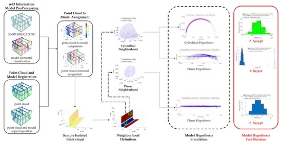
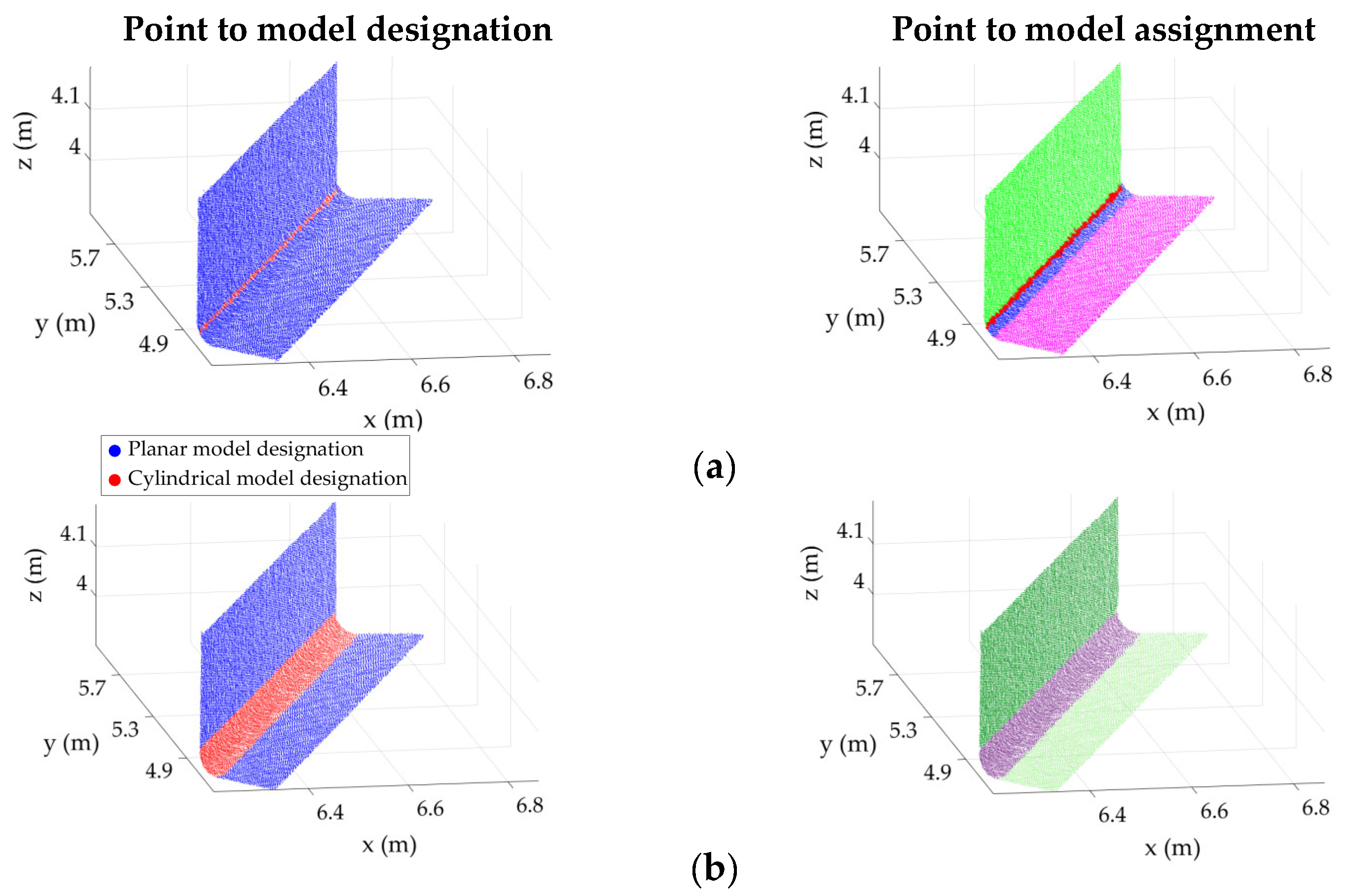
• Elemental classification of the design information model (Figure 1c), which is the process of labeling and detecting every element within the designed model based on criteria such as functional type and surface geometry. The surface geometry information related to the element type already exists within BIM and the industry foundation class (IFC) models [4,5] and, if available, can be used directly. In other cases, particularly when only 3D CAD models exist, the STereoLithography (STL) file format can be deployed, which approximates CAD object surfaces with triangular planes [20]. To further group triangular planes of the same surface together, a mesh segmentation process can be deployed, such as that proposed in [21,22,23]. The output of this stage is presented visually in Figure 1c, where each element is separated and shown with a unique color.
• Superimposition of the point cloud and the classified model (Figure 1d), which involves the registration of the coordinate systems of the point cloud and the model. To perform point-cloud-to-model registration, at least three non-colinear point correspondences between the model and the point cloud are necessary [24]. In the presence of a construction error, which is a reasonable assumption, given the statistics related to rework due to poor construction [25], it is recommended that we use identifiable and signalized targets on pre-surveyed site control points to perform the registration [16,26]. In cases where construction errors are less prominent, iterative closest point (ICP) registration of the point cloud and the closest surfaces on the model can be performed through methods such as the scan vs. BIM proposed in [20].
• Point-cloud-to-model comparison and assignment, which is used to aid with the assignment of the point cloud to the model elements. In the case of negligible construction errors, the distance of the point to the closest element can be used to determine correspondence, which is the metric used in the scan vs. BIM of [20]. A distance threshold must then be deployed to reject far points. Figure 1e shows an example of a heatmap used to visualize the distance of the points to the closest classified elements. Figure 1f presents the resulting point-cloud-to-element assignment with an arbitrarily defined distance threshold of 50 mm. In other cases, where possible local construction errors exist (e.g., a set of elements are incorrectly constructed or assembled), the correct assignment may require the use of additional information, such as point neighborhood behavior [26], curvature [27], color [28], or intensity [29].

The output of stage 3 above can then be employed for progress monitoring [16,17], dimensional quality checking [16], 3D BIM updating [18], and digital twinning [19].

1.2. Study Objectives, Scope, and Structure

The goal of this study is to present the best practices, along with new algorithmic developments, to automate the FIM process using point clouds, given a designed n-D information model. The presented state-of-the art methods describe the well-regarded scan vs. BIM [20], Reconstruct Inc. [17,30], Verity [31], entropy-based local point neighborhood definition [32,33], and random sample and consensus (RANSAC) shape detection [34]. Predicated on the gaps in the present methods, the new algorithms include leading developments for (i) point cloud vs. model comparison, (ii) robust point neighborhood definition, and (iii) Monte-Carlo-based point-cloud-to-model surface hypothesis testing. The scope of this study is to focus particularly on methods to solve stage 3 (and to a lesser extent stage 2) of the framework presented in Section 1.1 (Figure 1e,f) using only the geometric primitives (i.e., Cartesian coordinates) of the point clouds. The emphasis is on direct frameworks, which are generalizable, are robust to changes in scenery and point cloud type, and do not contain subjectively defined thresholds. To this end, the remainder of the manuscript is structured as follows:

• Section 2 describes the spatial uncertainty of point clouds and the necessity to incorporate this spatial uncertainty within a successful point cloud processing framework.
• Section 3 introduces point cloud processing when construction errors can be considered negligible. A new process for a point cloud vs. BIM is proposed, along with a demonstration of its effectiveness on real-world point clouds.
• Section 4 reveals the basic considerations for analysis of point clouds when the impact of construction errors cannot be neglected. New methods for point cloud neighborhood definition, surface-hypothesis-based classification, and surface segmentation, along with demonstrated real-world examples, are thoroughly discussed.
• Section 5 summarizes the findings and provides avenues for further explorations.

2. Point Cloud Spatial Uncertainty

Point clouds can be acquired through different means, such as terrestrial laser scanners (TLS; Figure 2a), simultaneous localization and mapping (SLAM)-based mobile systems (Figure 2b), and structure-from-motion (SfM)-based photogrammetric 3D reconstruction (Figure 2c). Each point cloud collection technique has unique characteristics that impact the level of spatial uncertainty of each point measurement. A generic framework to automate point cloud processing for construction projects must, hence, incorporate the impact of point measurement uncertainties corresponding to the optical instrument [35]. Figure 2 sheds light on the importance of integrating the expected point measurement uncertainties within automated point-cloud-processing frameworks. Figure 2 (right) shows histograms of point height, which have been shown to be an effective tool in extracting flat slab floors and ceilings from point clouds [36,37]. The points in the vicinity of the mode of the histograms represent the points of the floor (base slab). For reference, the root-mean-square error (RMSE) of the points on the floor for each histogram is also shown. As illustrated, the RMSE changes from 3 mm for TLS (Figure 2a, right) to 20 mm for dense 3D reconstruction from smartphone cameras (Figure 2c, right). This shows that if, for instance, a fixed distance threshold of, say, 5 mm is adopted to assign points around the mode of the histogram as floors, 99% of the TLS and only 32% of the smartphone 3D reconstruction points will be identified as belonging to the floor. Therefore, a successful distance threshold (Figure 1f) must incorporate the expected point measurement uncertainties related to a particular point cloud instrument [16,26,38,39].

Given a calibrated point cloud collection instrument (assumption of modeled systematic errors), the point measurement uncertainties in the Cartesian coordinate system (i.e., spatial uncertainty [38]) can be modeled through the propagation of instrumental measurement errors, typically approximated to the first order [40]. For instance, in TLS, the spatial uncertainty of points must incorporate the raw instrumental measurement errors (e.g., range and angular errors; see Equation (11) of [36]) along with possible scan station registration errors in the case of multiple scans (see Equation (5) of [16]). For each point, the variance propagation process provides a 3 × 3 covariance matrix, ${\mathsf{\Sigma }}_X$, as a measurement of spatial uncertainty. Closed formulations of the 3D positional uncertainty, ${\mathsf{\Sigma }}_X$, as a function of instrumental measurement errors can be found in Maalek et al. [16] for TLS (Figure 1a), Zhengchun et al. [38] for the laser radar measurement system (LRMS), Mourikis and Roumeliotis [41] for SLAM-based instruments (Figure 1b), and Beder and Steffen [42] for SfM-based techniques (Figure 1c). For each point, $X_i$, the corresponding spatial uncertainty, ${\mathsf{\Sigma }}_{X_i}$, can be used to construct an error ellipsoid as follows:

$${\left(X-X_i\right)}^T{\mathsf{\Sigma }}_{X_i}^{-1}\left(X-X_i\right)\le {\chi }^2{}_{p,\alpha },$$

(1)

where ${\chi }^2{}_{p,\alpha }$, the amplification coefficient, is considered a chi-squared probability with confidence $p$ (in this study, $p=97.5\%$ is used) and $\alpha$ degrees of freedom ($\alpha =3$ for 3D data). Throughout the remainder of the manuscript, every point will be represented by its error ellipsoid using Equation (1).

2.1. Assumptions of Input Parameters

Before describing the methods of processing point clouds in Section 3 and Section 4, it is worth outlining the basic assumptions and available input parameters, as follows:

• The n-D designed information model is available, accurate and up-to-date with the latest change orders.
• It is expected that stages 1 and 2 of the typical point cloud processing, corresponding to Figure 1a–d, are reliably completed. This means that a point cloud from the field is acquired, the instrument by which the point cloud was collected is known, the elemental classification of the n-D designed information model is carried out, and an initial target-based registration of the point cloud and the model is performed.
• The point cloud instrument is assumed to be calibrated, containing no (or negligible) systematic error trends.
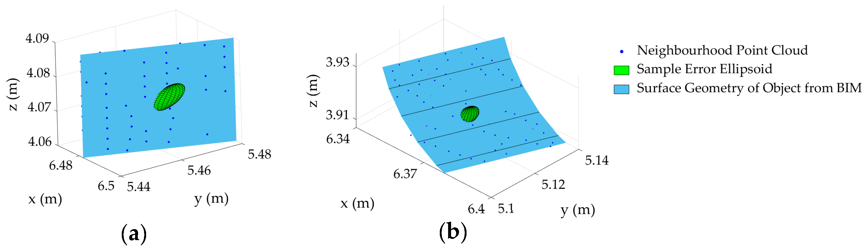
• The spatial uncertainty of each point is modeled, and the error ellipsoid as per Equation (1) is constructed for each point.

3. Point Cloud Analysis: Case of Negligible Construction Errors

This section describes the methods that can be incorporated when construction errors are considered negligible (for instance, in cases of reliable pre-fabrication [45] and/or 3D printing [11] processes). This suggests that the designed n-D model and the point cloud acquired from the constructed scene must comply with little to no construction errors. Therefore, given an initial reliable point-cloud-to-model registration, the problem of point cloud processing reduces to assigning the point to its closest element and rejecting points that are farther than a pre-defined threshold. This type of procedure was adopted for 3D-reconstructed photogrammetric point clouds in Golparvar-Fard [17] and for TLS point clouds within the scan vs. BIM of Bosche [20]. The two methods, however, differ in some points. For the photogrammetric case, since the positions and orientations of the images are estimated during the dense 3D reconstruction stage [46], Golparvar-Fard [17] proposed to perform a perspective projection of the 3D model with the same view angle at each camera position and orientation. The 3D model is now converted into a 2D image and superimposed onto the original image to enable pixel to model assignment within each image. The image pixel is assigned to the closest 2D model pixel. The conversion of the 3D model to a 2D image possesses some merits. First, since the positional uncertainties of the cameras have been already calculated during the SfM process, they can be incorporated within the assignment of each pixel to the corresponding model element in the image. Furthermore, the assignment is performed in 2D rather than 3D, which can be faster and, if required, can allow the use of the many available and established image-processing frameworks. The process will, however, lose efficiency when occlusions are present on-site due to the loss of information with dimensionality reduction of 3D to 2D. Therefore, additional steps, such as supervised learning, may be required to improve the pixel to model assignment in the existence of occlusions [47]. Furthermore, the process is only suited for images and cannot be generalized for point clouds acquired by other means, such as TLS.

The scan vs. BIM method [20] first generates a template-designed point cloud by parallel projection of the acquired point clouds onto the closest surfaces in the designed model. The method then performs an iterative closest point (ICP) registration between the point clouds and the designed template point clouds until convergence. At each iteration, only points within a distance threshold (a function of a constant distant, ${\epsilon }_{Const.}$, and the registration errors in the previous iteration) are used for registration and assignment. The method is attractive since it reduces the point-cloud-to-model assignment into a template-matching problem [48,49] and aims to also minimize possible target-based registration errors. The method, however, does not incorporate the impact of instrumental measurement errors pertaining to the point’s spatial uncertainties (see Section 2). Furthermore, ${\epsilon }_{Const.}$ was arbitrarily defined as 50 mm in the study, which may not be generic for all datasets (the impact of ${\epsilon }_{Const.}$ on the ICP registration will be demonstrated later). Finally, ICP registration is based on point-to-point correspondence, which is known to be less accurate than point-to-plane registration [50,51]. Therefore, direct point-cloud-to-plane registration can not only improve the registration accuracy (and the convergence rate) but also remove the necessity for generating the designed template point cloud altogether.

3.1. A New Generic Process for Point Cloud vs. Model

With due consideration of the limitations of the aforementioned methods, a new generic method, presented in Algorithm 1, given the assumptions and inputs of Section 2.1, is proposed as follows:

Algorithm 1 Point Cloud vs. Model

Iterative improvement of the point-cloud-to-model registration: 1.1. Assign points to corresponding planar surfaces in the model as below: 1.1.1. For each point, find the closest planar surfaces whose distances to the point are smaller than the semi-major length of the error ellipsoid (see reference [16] Algorithm 5-step 2). 1.1.2. Assign the point to the closest planar surface that intersects the error ellipsoid (ellipsoid-surface intersection is treated in Appendix A). 1.2. For each planar surface, find the inlier points of the set of points, which were assigned to the plane in step 1.1, using Algorithm A1 (Appendix B). 1.3. Perform the closed-form point to plane registration, proposed by Khoshelham [51] to transform the inlier points onto the corresponding model planes. 1.4. Transform all points using the registration parameters of step 1.3. 1.5. Perform steps 1.1–1.4 until the points used for registration between two consecutive iterations remain constant. Assignment of non-planar points to non-planar model surfaces: 2.1. Identify the points which were not assigned to a planar surface (the remaining points after step 1). 2.2. Find the closest non-planar surface that intersects the error ellipsoid of the point (Appendix A). 2.3. For each surface in the model, perform the robust model fitting of Algorithm A1 (Appendix B) to find the inlier points. 2.4. Assign the inlier points to the corresponding surface and exit the algorithm.

In Algorithm 1, given a reliable registration, a point is assigned to a surface if the following two conditions are met:

• Its error ellipsoid intersects the surface. This is schematically shown in Figure 3a,b for planar and cylindrical surfaces, respectively. The intersection of ellipsoids and common surfaces such as planes, cylinders, spheres, and ellipsoids will be covered in Appendix A.
• The point follows the pattern of the assigned surface (an inlier point). The algorithm for detecting inlier points, given a particular model, will be discussed in Appendix B.

Step 1 of Algorithm 1 involves an iterative process to improve the registration in the absence of a reliable initial target-based registration (similar to the ICP of [20]). The registration process, however, only uses planar surfaces. Point-to-plane registration is used particularly since it is known to be accurate [50], and a reliable closed-form linear solution to the point-to-plane registration problem already exists [51], unlike, say, cylinder-based registration, which is non-linear at best [52].

3.2. Demonstration 1: Comparison of Scan vs. BIM and Point Cloud vs. Model

3.2.1. Experimental Setup

Point cloud data from one rectangular concrete column with rebars on top, acquired from a building construction project, were used (Figure 4a; data presented in [16,36]). To simulate a model with no construction errors, the following processes were carried out:

• The point cloud of the sample column was subjected to a rigid body transformation (translation and rotation; Figure 4b).
• The as-built model of the rectangular column surfaces as well as the cylindrical rebars for the transformed point cloud were generated manually using FARO As-built Modeler software [53] (Figure 4c,d).
• The original point cloud was then superimposed onto the as-built model of the transformed point cloud for comparison (Figure 4e).
• The proposed point cloud vs. model was compared to the scan vs. BIM method. The scan vs. BIM method was performed using four distance configurations with ${\epsilon }_{Const.}$ changing from 50 mm to 125 mm in 25 mm increments.

3.2.2. Results: Registration Error Comparison

Figure 5 shows the results of the registration error in each iteration using our method and the four configurations of scan vs. BIM. Two main observations were made from the results shown in Figure 5. First, scan vs. BIM appears to be considerably impacted by the change in ${\epsilon }_{Const.}$. In our data, ${\epsilon }_{Const.}$ of 100 mm and 125 mm were the most optimum and produced almost identical registration results, whereas ${\epsilon }_{Const.}$ of 50 mm produced poor registration results. The second observation was that the proposed method, which is independent of arbitrarily defined thresholds, significantly outperformed scan vs. BIM, even at the most optimum distance of ${\epsilon }_{Const.}=100 \mathrm{mm}$. In fact, the proposed method after the first iteration produced better results than the converged scan vs. BIM after 30 iterations. The proposed method converged after only four iterations and produced a final registration error of 0.9 mm, about four times better than the best scan vs. BIM, which produced a registration error of 3.2 mm after 30 iterations.

3.2.3. Results: Quality of Point-to-Surface Assignment

Given the impact of ${\epsilon }_{Const.}$ on registration errors, it is also important to evaluate the quality of the point-to-model assignment for each method. Here, the precision, recall, accuracy, and F-measure, introduced in [54], are used to define the quality of the point-cloud-to-model assignment.

Table 1. Summary of the quality of point-cloud-to-model assignment using different methods.

Method	Precision	Recall	Accuracy	F-Measure
Scan vs. BIM −5 mm	87.9%	76.9%	69.7%	82.1%
Scan vs BIM −75 mm	98.8%	87.5%	86.6%	92.8%
Scan vs. BIM −100 mm	100.0%	87.5%	87.5%	93.3%
Scan vs. BIM −125 mm	100.0%	86.8%	86.8%	92.9%
Proposed point cloud vs. BIM	98.8%	99.9%	98.7%	99.3%

Bold numbers represent the best value in each column.

provides a summary of the assignment quality for each method. The scan vs. BIM at ${\epsilon }_{Const.}$ of 50 mm achieved comparatively poor results in both precision (type I errors) and recall (type II errors). The scan vs. BIM, however, appeared to become more robust to type I errors (i.e., the correct detection of points belonging to the surface) as the ${\epsilon }_{Const.}$ increased from 50 mm to 125 mm. In fact, scan vs. BIM slightly outperformed our proposed method in type I errors. Our method, however, considerably outperformed scan vs. BIM in type II errors (i.e., the correct rejection of points not belonging to the surface). The latter is a consequence of the robust inlier detection (Appendix B), which was used within the point-to-surface assignment process to reject outlying points.

The robustness of our proposed method to type II errors compared to scan vs. BIM with ${\epsilon }_{Const.}=100 \mathrm{mm}$ is visually presented in Figure 6. It can be observed that many points of both planar and cylindrical surfaces, which are within the distance threshold of ${\epsilon }_{Const.}=100 \mathrm{mm}$, are incorrectly assigned to the surface. In our method, other than the fact that the distance threshold (error ellipsoid) is systematically defined based on the spatial uncertainty of each point, a robust surface fitting is performed to further reduce the impact of outliers and consequentially improve type II errors.

3.3. Constraint for Negligible Construction Error

The aforementioned methods, e.g., scan vs. BIM, which use a distance metric to assign points to their corresponding elements, can only produce reliable results when the constraint of negligible construction error is met. This is attributed to the fact that the presence of construction errors cannot be quantified a priori, i.e., before the point cloud is analyzed. The existence of construction errors will hinder these methods in the following two ways:

• Distance metric: Since the distance threshold is the basis for the assignment or rejection of a point to an element, without a priori knowledge of the construction errors, the threshold will be a guess at best. The impact of the subjective definition of ${\epsilon }_{Const.}$ (introduced in the previous section), even for the case without construction errors, was thoroughly discussed in Section 3.2.
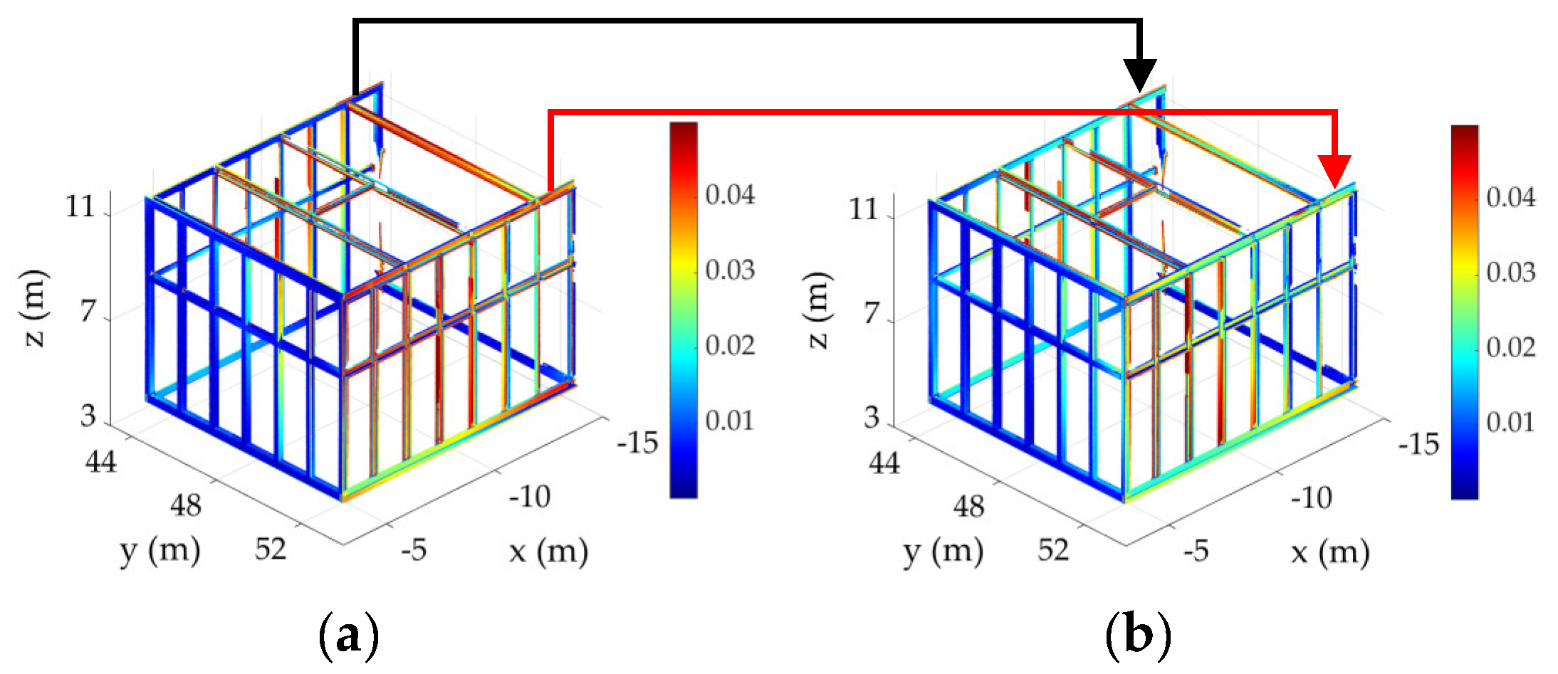
• Iterative registration: Since iterative ICP registration is performed on all elements, those elements with additional construction errors might also be used within the least-squares registration. Similar to any least-squares adjustment in the presence of outliers [55], the outlying elements due to construction errors will negatively impact the overall registration quality. An example of this phenomenon for scan vs. BIM is provided in Figure 7. In this example, even though the overall registration RMSE improved from 21 mm in Figure 7a to 18 mm in Figure 7b, the registration process, for example, sacrificed the accuracy of the element, shown with the black arrow, to accommodate the element, shown in red. However, Figure 7a represents the correct point-to-model distance, and hence, the element, shown in red, must not be allowed to influence the registration. It is possible to solve this problem by adopting a local registration and matching strategy, which will be treated in Section 4.

4. Point Cloud Analysis: Existence of Construction Errors

A construction error is defined, here, as the possibility of a set of model elements to be installed and built in the field incorrectly, particularly in terms of their positions, orientations, and/or dimensions. The problem of damaged elements, where the geometry of the element is altered (e.g., a bent rectangular column), was not considered in this study. In the existence (or speculation) of construction errors, given an initially reliable registration of the point cloud and the model, each element can be treated separately and point cloud processing can be carried out locally (unlike the global methods described in Section 3). To this end, for each element, a local set of points is first isolated [26] using a relaxed local tolerance to account for possible construction errors (say 200 mm). The assignment of the isolated points to the model elements can then be treated in one of the following two ways or a combination of the two:

• Fitting the model directly to the point cloud, which aims at finding the group of points that match the geometry of the element. This can be accomplished by means of heuristic methods such as template matching [48,49], and robust least-squares adjustment [26,55,56].
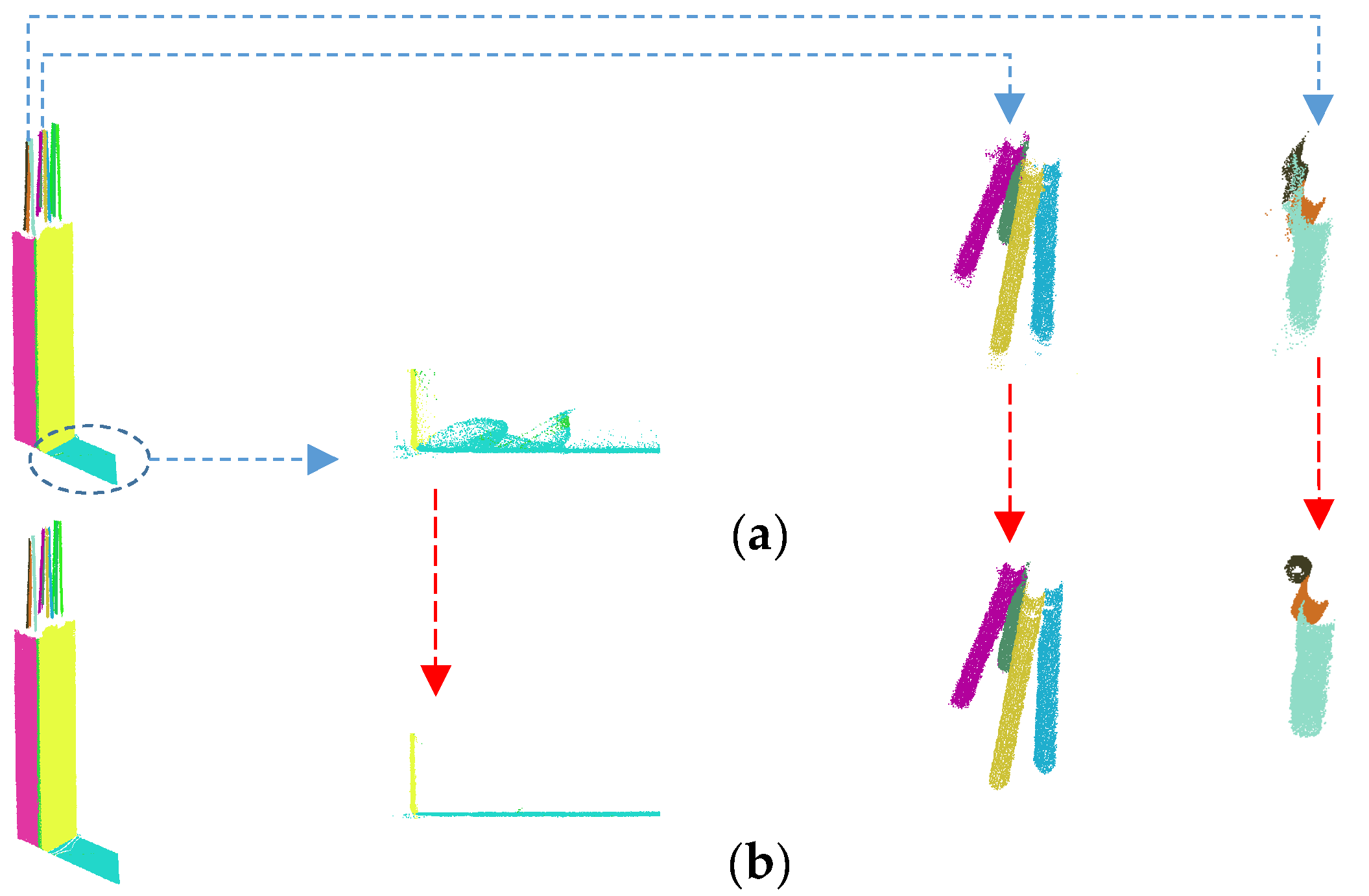
• Local point-cloud-to-model hypothesis testing, which aims at finding the points that locally follow the pattern of the element’s geometry.

The difference is that the second class of methods incorporates the local geometry of each of the isolated points to enable point-to-model assignment with higher confidence. This additional local information may become particularly useful when assigning non-analytical shapes in the presence of outliers. To provide some perspective, an example of a rectangular hollow structural section (HSS), analyzed using Verity [31], the first approach, is shown in Figure 8. As illustrated, due to the presence of outliers, the heuristic search of Verity found a non-optimal and incorrect transformation for the HSS element (Figure 8b). This is particularly attributed to the fact that only a limited combination of points (in this case, 1000 combinations) is used and the combination satisfying some decision criteria (e.g., the highest consensus [57]) is selected. Additional combinations might improve the results but increase the computation time without guarantee of optimality [58]. Local neighborhood information, such as curvature, may provide additional means to support the point-cloud-to-model assignment [27]. The remainder of this section is dedicated to presenting new methods to address class 2 local point-cloud-to-model hypothesis testing.

4.1. Local Point-Cloud-to-Model Hypothesis Testing

Given the geometric representation of the element in the design model, the problem is to find the sets of points that locally follow the element’s geometric pattern. The problem is solved using Algorithm 2, presented below:

Algorithm 2 Point-Cloud-to-Model Hypothesis Testing

Find the local neighborhood of each point (Figure 9b and Figure 10b). For each neighborhood, estimate the best fit parameters of the element’s surface geometry (e.g., best-fit plane Figure 9c and Figure 10c, cylinder Figure 10e, and so on) and record the RMSE of the fit, $RM{S}_{Real}$. If an element consists of more than one surface geometry (e.g., HSS with cylindrical and planar surfaces), perform the remaining steps on the model with the lowest RMSE in accordance with the Bayesian information criterion [59]. Determine the distribution of the RMSE (Figure 9d and Figure 10d,f) if the points were to follow the hypothesized model as follows: 3.1. Project the points onto the best-fit model (perspective projection is recommended for optical instruments such as perspective cameras and TLS). 3.2. Subject the projected points to additive measurement errors (Figure 9c and Figure 10c,e) by simulating a random point within the error ellipsoid of the original point to account for the spatial uncertainty of Equation (1). 3.3. Calculate the RMSE of the best-fit to the points subjected to spatial uncertainties. 3.4. Perform steps 3.1 through 3.3 $N_T$ times to develop the distribution of the RMSE. From step 3, record the maximum RMSE ($RM{S}_{Max}$), mean of the RMSE ($RM{S}_{mean}$), and standard deviation of the RMSE (${\sigma }_{std.}$) of the simulated RMSE distribution. The point belongs to the surface type if and only if the following condition is met: $$RM{S}_{Real}\le \max \left\{RM{S}_{Max}|RM{S}_{mean}+3{\sigma }_{std.}\right\},$$ (2)

Algorithm 2 uses the surface geometry of the element, along with the spatial uncertainty of the points, to simulate a probability distribution of the RMSE if the points were to follow the hypothesized geometry. The point will be designated to the geometry if and only if its RMSE complies with that of the simulated distribution. The use of Monte Carlo simulation, here, enables the generation of the distribution of the RMSE, which in general form is challenging to formulate analytically (e.g., finding the distribution of the smallest eigenvalue [60]). Furthermore, the information regarding the distribution of the best-fit parameters, such as covariance and the mean of the distribution of the surface normal, can also be estimated during the process, which is shown to be an asset in systematically determining the correct threshold for surface segmentation [36].

Figure 9 shows the process, described in Algorithm 2, for a neighborhood of points following a planar pattern. It can be observed from Figure 9d that the RMSE of the original point cloud neighborhood of Figure 9b is much smaller than even the mean of the probability distribution function of the RMSE of the simulated points, indicating that the point considered in Figure 9 satisfies Equation (2) and follows a planar pattern. This is, in fact, not the case for the cylindrical neighborhood, shown in Figure 10. For the cylindrical neighborhood, if the points are projected onto the best-fit plane, the RMSE of the best-fit plane to the cylindrical points considerably exceeds the maximum of the probability distribution of the RMSE of the simulated planar points (Figure 10d). Alternatively, if a cylinder is fitted to the cylindrical points, the RMSE of the best-fit cylinder is within the probability distribution of the RMSE of the simulated cylindrical surface and satisfies the requirement set in Equation (2) (Figure 10f). Therefore, the point considered in Figure 9 will be classified as a plane and the point considered in Figure 10 will be classified as a cylinder.

Algorithm 2 is non-parametric and only requires the spatial uncertainties of the points from Equation (1) as well as the type of geometric surface from the element’s design information model. Once the points are designated (classified) to the desired surface model (e.g., plane, cylinder, etc.) using Algorithm 2, Algorithm 1 (or template matching [48]) can be used on only the designated points for the final point-to-model assignment. The final considerations for Algorithm 2 are to define a reliable neighborhood around each point, and to determine the required number of Monte Carlo iterations, $N_T$, to form a reliable distribution of RMSE, which are discussed next.

4.2. Robust Neighborhood Definition

The neighborhood of points can be defined as fixed [36] or variable [32,33]. For the fixed neighborhood case, either a fixed radius around the point or a fixed number of neighboring points is considered. In practical settings, since the local point cloud resolution and density vary throughout the dataset, a fixed neighborhood cannot capture the impact of the change in point density effectively. Variable neighborhood sizes are generally more effective in capturing the local point density variations and consequentially better representing the behavior of the neighborhood of the points [32,33]. The most reliable methods for adaptively selecting the neighborhood of each point [32,33] use basic principles from decision and information theory [61] to find the set of points achieving the minimum information entropy. Theoretically, the set of points with the smallest entropy will contain the maximum information. To this end, a range of neighborhoods is considered and that achieving the lowest information entropy is selected [32,33]. The two methods presented in [32,33] differ in their definitions of features used to formulate the entropy function with Weinmann’s formulation [32], achieving slightly better results.

The problem of a variable neighborhood can be formulated in robust statistical sense as finding the set of points whose determinant of the covariance matrix is minimum (MCD [55,62]), which is the set of points with the least outliers. It turns out that minimizing the determinant of the covariance matrix also minimizes the differential entropy for Gaussian distributions (Equation (1) in [63]), which is also consistent with the principles of decision and information theory [61]. Hence, the optimum neighborhood can be cons as that achieving the MCD. However, to compare the MCD as the neighborhood size increases, the data must be normalized; otherwise, larger neighborhoods will produce greater covariance determinants. Here, the data are normalized such that the total variance, the sum of the eigenvalues of the covariance matrix, equals unity. The process is formulated using Algorithm 3, given the starting radius (or the number of points) ($r_{min}$), the final radius ($r_{max}$), and the sampling step (${\delta }_r$) for each point as follows:

Algorithm 3 Robust Neighborhood Definition

Generate the sampling radius: $\left\{r_i=r_{min}+i.{\delta }_r|i=0:1:\frac{r_{max}-r_{min}}{{\delta }_r}\right\}$. For each sampling radius, $r_i$, find the closest points to the point of desire within the spherical radius, $r_i$. Calculate the eigenvalues of the covariance matrix of the set of points from step 2, ${\mathsf{\Lambda }}_{r_i}=\left({\lambda }_1,{\lambda }_2,{\lambda }_3\right)$.

4. Calculate the normalized MCD, $E_{MCD}$, as follows: $$E_{MCD}={\prod }_{k=1}^3\frac{{\lambda }_k}{{\lambda }_1+{\lambda }_2+{\lambda }_3},$$ (3)

5. Select the $r_i$ that receives the smallest $E_{MCD}$.

4.3. Demonstration 2: Evaluation of the Point-to-Model Quality

This section involves the assessment of the effectiveness of the proposed methods on a point cloud of the sample HSS member of Figure 9a and Figure 10a, acquired using the Leica HDS6100 TLS [43]. The sample point cloud consists of two planar surfaces and a cylindrical fillet. Four experiments are described next, namely robust neighborhood evaluation, impact of Monte Carlo iteration, impact of neighborhood size, and comparison with random sample and consensus (RANSAC) [34,57].

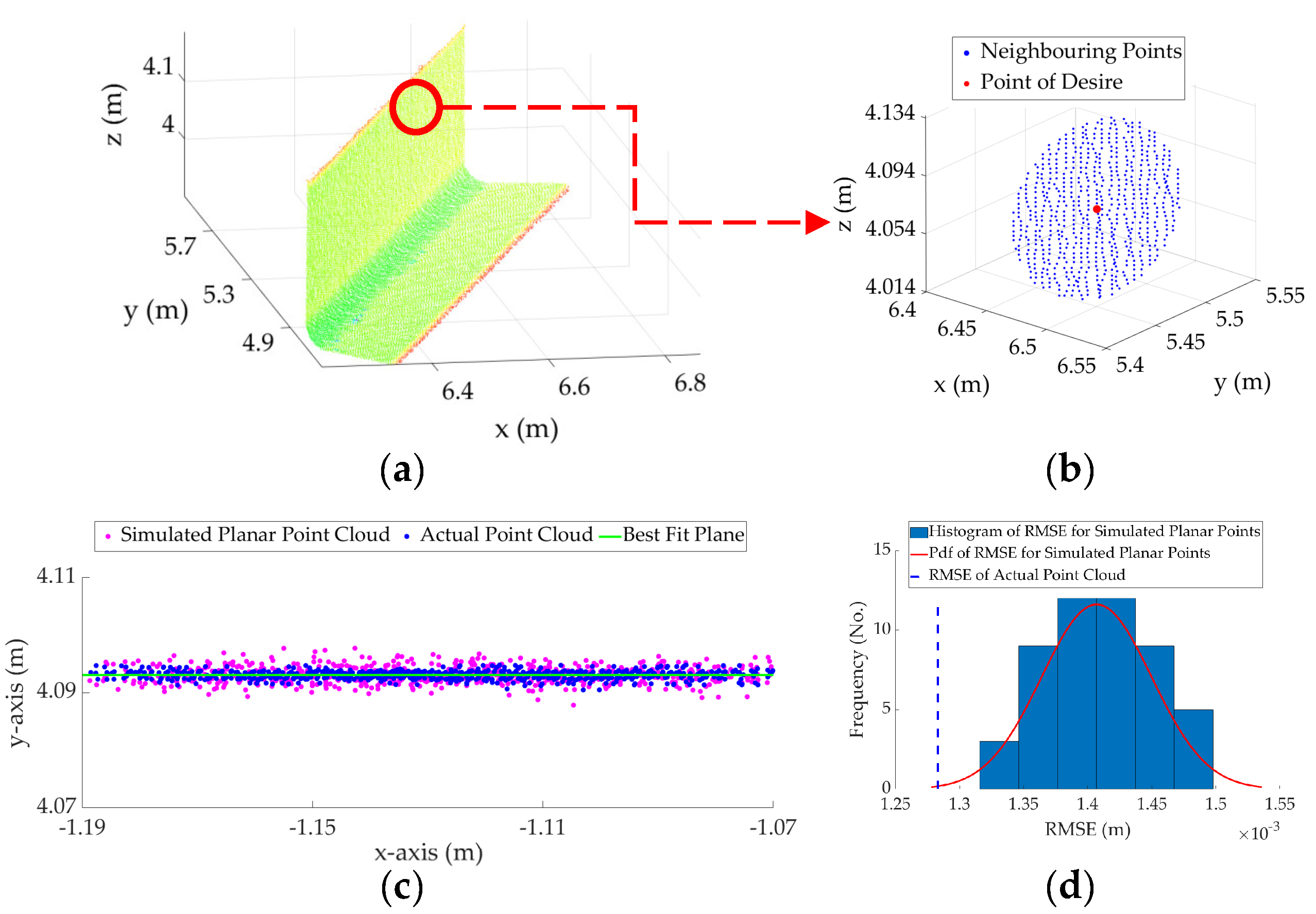
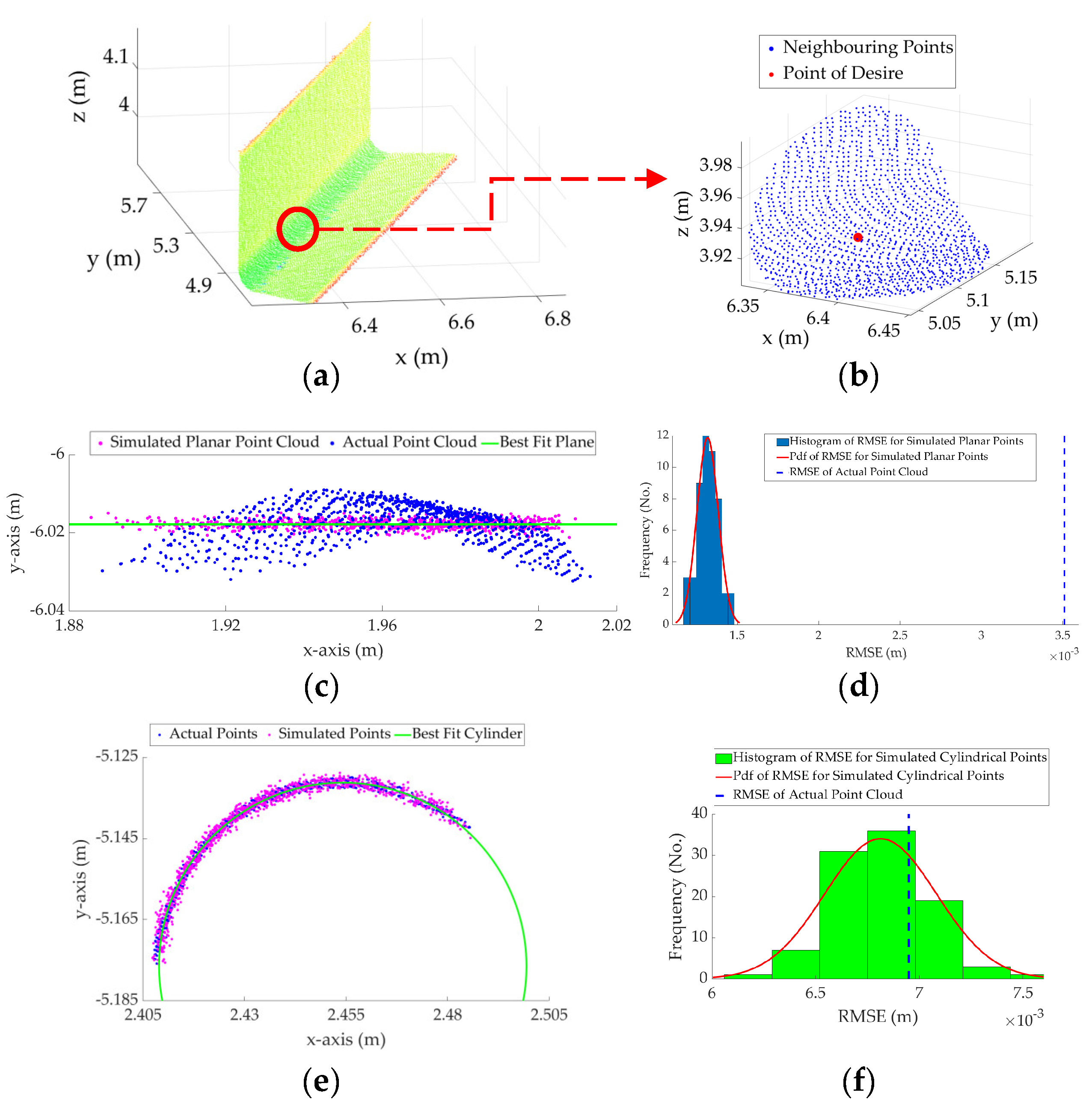
4.3.1. Robust Neighborhood Evaluation

The robust neighborhood definition of Algorithm 3 is compared to the reliable variable neighborhood definition of Weinmann [32] for the data presented in Figure 9a and Figure 10a. The neighborhood radius was set to change from 20 mm to 70 mm in 1 mm increments. The results of the defined neighborhood radius using Weinmann’s [32] and our methods are visually shown in Figure 11b,c, respectively. As illustrated, both methods produce similar patterns of neighborhood sizes for the planar (larger neighborhoods) and cylindrical (smaller neighborhood) regions. Our method, however, appears to be more consistent with defining the neighborhood of points for the planar and cylindrical regions. For instance, Weinmann’s method finds a smaller neighborhood for the points of the same planar surface on the edges of the surface (marked in black oval), whereas ours provides a consistent neighborhood around the points of the same surface. Further observations can be made from the green ovals, which are again from the same planar surface. Overall, the accuracy of the angle between the estimated normal and the ground truth normal vector was around 0.2° and 0.6°, using the proposed and Weinmann’s methods, respectively.

4.3.2. Impact of Monte Carlo Iteration

This experiment was designed to quantify the impact of the number of iterations, $N_T$, used to generate the probability distribution of the RMSE in Algorithm 2. To this end, Algorithm 2 in combination with Algorithm 3 was applied to the sample data, with $N_T$ increasing from 25 to 1000. The quality of the planar and cylindrical classification (precision, recall, accuracy, and F-measure) was quantified and recorded for each iteration. Figure 12 shows the quality of the classification as the number of iterations increases. It can be observed that the precision, recall, accuracy, and F-measure remain relatively constant as the number of iterations increases from 50 to 1000. The precision and, consequentially, the accuracy and F-measure were, however, relatively lower with 25 iterations compared to 50 iterations. Therefore, 50 iterations appear to be an appropriate choice for the number of iterations. $N_T=50$ was also tested on the dataset shown in Figure 4a, with similar results.

4.3.3. Impact of Neighborhood Size

In Section 4.3.1, it was established that the proposed neighborhood definition can provide accurate results, particularly to estimate the surface normal, in comparison to an established variable neighborhood definition method. Here, the impact of fixed neighborhood sizes on the quality of the point-to-model designation using Algorithm 2 is evaluated. To this end, the neighborhood size was changed from 25 mm to 75 mm in 5 mm increments and the precision, recall, accuracy, and F-measure were recorded. Figure 13 shows the quality of planar and cylindrical classifications of Algorithm 2 ($N_T=50$) using different fixed neighborhood sizes. The dashed lines show the classification quality using the robust neighborhood of Algorithm 3. As illustrated, the size of the neighborhood considerably impacts the quality of the classification. The precision appears to reduce as the neighborhood size increases. The recall, on the other hand, increases as the neighborhood size increases. Due to this counteraction between precision and recall, the F-measure and accuracy peak at the neighborhood size of around 30 mm. The robust neighborhood using Algorithm 3 provided a lower precision (indication of type I errors) but a relatively higher recall (indication of type II errors) compared to the neighborhood size of 30 mm. In fact, the F-measure and the recall using the robust neighborhood outperformed all neighborhood sizes of a fixed radius. The considerable impact of the neighborhood size on the classification quality also demonstrates that if the data were to be isotopically scaled, the most optimum fixed neighborhood size (in this case 30 mm) must also be scaled. Therefore, a fixed neighborhood cannot possibly provide the same point-to-model designation quality with models of different sizes and with varying point cloud densities.

4.3.4. Comparison with RANSAC

The proposed method for point designation to planar and cylindrical surfaces was compared to the established RANSAC methodology of [34], which was specifically designed for shape detection, and implemented in the popular software CloudCompare [64]. The results of the two methods are presented in Figure 14. Figure 14 (left) shows the results of the surface designation, where points detected as planar are shown in blue and points following cylindrical patterns are shown in red. As illustrated in Figure 14a (left), although the considered RANSAC method was successful in detecting most planar points, it failed to correctly classify most of the cylindrical points. In fact, the method incorrectly classified most cylindrical points as planar. Our method, shown in Figure 14b (left), on the other hand, correctly classified both planar and cylindrical points. Figure 14 (right) shows the results of the planar and cylindrical segmentation using the considered RANSAC method (Figure 14a, right) and the proposed method combined with the robust complete linkage segmentation of Maalek [36] (Figure 14b, right).

The precision, recall, accuracy, and F-measure for both methods are provided in

Table 2. Summary of the quality of point-to-model assignment using our method and RANSAC.

Method	Precision	Recall	Accuracy	F-Measure
RANSAC CloudCompare	94.7%	83.9%	81.3%	89.0%
Proposed point-to-model assignment	97.7%	99.0%	97.4%	98.4%

Bold numbers represent the best value in each column.

. Our proposed methods (Algorithms 2 and 3) and RANSAC of [34] achieved F-measures of 98.4% and 89.0%, respectively, which demonstrates the higher performance of the proposed methods. Our method particularly outperformed RANSAC in type II errors related to the correct assignment of points to cylindrical surfaces (as demonstrated from the recall rate).

4.4. Demonstration 3: Comparison with Local Scan vs. BIM

To complete the picture of local assignment of point clouds to a desired element in the presence of possible construction errors, an HSS member and the locally surrounded points of Figure 15a are considered. Even though the overall point cloud and model are registered, the HSS member of Figure 15a is locally not correctly registered to its corresponding points due to construction errors. The registration and assignment of the HSS model element to point cloud was carried out once using a local implementation of scan vs. BIM (Figure 15b) and again using Algorithms 1–3 (Figure 15c), for comparison. Using our method, first Algorithms 2 and 3 are applied to detect planes and cylinders. Algorithm 1 is then utilized to register and match the model to the correct point cloud. As illustrated in Figure 15b, local implementation of scan vs. BIM contains many Type II errors. The proposed combination of Algorithms 1–3, on the other hand, achieved considerably higher robustness to Type II errors compared to scan vs. BIM. In terms of point cloud to model registration, scan vs. BIM and our method achieved RMSE of 7.9 mm and 2.7 mm, respectively. The proposed methodology, hence, outperforms the local implementation of scan vs. BIM for both point cloud assignment and registration in data with local construction errors.

5. Discussion on the Summary of Findings

Two categories of methods were presented, critically assessed, and analytically compared to solve point cloud assignment with the following properties:

• Negligible construction errors, which considered the methods of scan vs. BIM [20] and Reconstruct Inc. [17,30] from previous literature, and the newly developed Algorithm 1 for point cloud vs. model comparison; and
• Existence (or speculation) of construction errors, which discussed the approaches taken by Verity [31], entropy-based local point neighborhood definition [32,33], and RANSAC shape detection [34] from existing studies, and the newly proposed Algorithms 2 and 3 for point-cloud-to-model hypothesis testing.

In the case of negligible construction errors, a generic point cloud vs. model framework was proposed, Algorithm 1, which first performs an iterative global point-to-plane registration between the point cloud and the model. The process then assigns the points to the closest model elements that intersect with the point’s error ellipsoid (representative of spatial uncertainty). It was shown that the popular scan vs. BIM is considerably influenced by the choice of the distance threshold, with the point assignment F-measure changing from 82.1% to 93.3% with different thresholds. The proposed point cloud vs. model method, which is not a function of a subjectively defined threshold, achieved an F-measure of 99.3%, outperforming scan vs. BIM in all considered thresholds.

In the existence of construction errors, it was argued that the local behavior of each point can provide additional information to aid with the point-cloud-to-model assignment. To this end, a new generic method was proposed to designate points to classes of surface geometries of each element in the designed model. The method first simulates point clouds of the surface geometry using the spatial uncertainty of each point and then decides whether the neighborhood of the point follows the pattern of the considered class of geometry. The method is non-parametric and generic; however, it requires a process for neighborhood definition. Therefore, a new method for neighborhood definition was proposed that is consistent with both robust statistics and information theory. The normal vectors, estimated using the proposed robust neighborhood definition, were found to achieve an angular error of only 0.2° on average, compared to the ground truth normal vectors. The proposed point-to-model hypothesis testing, for both cylinders and planes, achieved an F-measure of 98.4% on a real-world point cloud from an HSS member. It was also shown that the proposed method outperformed established RANSAC methods, particularly in the correct assignment of points to cylindrical surfaces. Finally, the efficient combination of Algorithms 1–3 on data with visible local construction error was compared to a local implementation of scan vs. BIM. It was observed that the proposed method outperformed local scan vs. BIM in both point cloud to model assignment and registration.

6. Concluding Remarks and Avenues for Future Exploration

The automated analysis of point clouds, acquired from construction projects, enables frequent measurement and reporting of the project’s performance, which is imperative to promote continual improvement. To this end, the study focused on the methods to assign point clouds to their corresponding elements, given a reliably designed n-D model, the spatial uncertainty of the point clouds and reliable registration between the model and the point cloud. The methods were further sub-categorized to address field conditions with negligible construction errors and the existence (or speculation) of construction errors.

Given some of the assumptions presented in this study, the following remain possible avenues for further investigation:

• Automated spatial uncertainty estimation: Currently, the proposed frameworks are predicated on the formulation of the error ellipsoid of each point a priori. While this can be accomplished for most instruments, it would still be attractive to formulate this spatial uncertainty automatically and directly from the point cloud.
• Closed formulation of distribution of the RMSE: Algorithm 2 involved simulating multiple sets of points to generate the distribution of the RMSE. Formulating this RMSE in closed form will remove the requirement for simulating the multiple sets of points, which, depending on the formulation, might improve computational efficiency.
• Point cloud assignment in the presence of damages: This study focused on errors during construction, including orientational, positional, and dimensional errors of a particular element. Automatic assignment of points to damaged elements, such as cracks and deformations, will be an interesting avenue for further exploration.
• Point cloud registration comparison: A comparison of the point cloud registration method proposed in Algorithm 1 with supervised learning methods such as that proposed in [65] could be of interest to some researchers.

References

1. Fu, C.; Aouad, G.; Lee, A.; Mashall-Ponting, A.; Wu, S. IFC model viewer to support nD model application. Autom. Constr. 2006, 15, 178–185. [Google Scholar] [CrossRef]
2. Ding, L.; Zhou, Y.; Akinci, B. Building Information Modeling (BIM) application framework: The process of expanding from 3D to computable nD. Autom. Constr. 2014, 46, 82–93. [Google Scholar] [CrossRef]
3. Jung, Y.; Joo, M. Building information modelling (BIM) framework for practical implementation. Autom. Constr. 2011, 20, 126–133. [Google Scholar] [CrossRef]
4. Autodesk. AUTODESK Revit IFC Manual: Detailed Instructions for Handling IFC Files; Autodesk: San Rafael, CA, USA, 2018. [Google Scholar]
5. BuildingSMART. IFC Standard. Available online: https://standards.buildingsmart.org/IFC/RELEASE/IFC4/ADD1/HTML/schema/ifcgeometricmodelresource/lexical/ifcfacebasedsurfacemodel.htm (accessed on 6 February 2021).
6. Koo, B.; Fischer, M. Feasibility Study of 4D CAD in Commercial Construction. J. Constr. Eng. Manag. 2000, 126, 251–260. [Google Scholar] [CrossRef] [Green Version]
7. Lee, X.S.; Tsong, C.W.; Khamidi, M.F. 5D Building Information Modelling—A Practicability Review. In Proceedings of the MATEC Web of Conferences EDP Sciences, Amsterdam, The Netherlands, 23–25 March 2016; Volume 66, p. 00026. [Google Scholar]
8. Kang, J.; Ganapathi, A.; Lee, J.; Faghihi, V. Robotic total station and BIM for quality control. In eWork and eBusiness in Architecture, Engineering and Construction, Proceedings of the European Conference on Product and Process Modelling (ECPPM), Reykjavik, Iceland, 25–27 July 2012; Taylor & Francis Group: London, UK, 2012. [Google Scholar]
9. Chi, H.L.; Kang, S.C.; Wang, X. Research trends and opportunities of augmented reality applications in architecture, engineering, and construction. Autom. Constr. 2013. [Google Scholar] [CrossRef]
10. Ruwanpura, J.Y.; Hewage, K.N.; Silva, L.P. Evolution of the i-Booth© onsite information management kiosk. Autom. Constr. 2012. [Google Scholar] [CrossRef]
11. Tay, Y.W.D.; Panda, B.; Paul, S.C.; Noor Mohamed, N.A.; Tan, M.J.; Leong, K.F. 3D printing trends in building and construction industry: A review. Virtual Phys. Prototyp. 2017, 12, 261–276. [Google Scholar] [CrossRef]
12. Petersen, P.B. Total quality management and the Deming approach to quality management. J. Manag. Hist. 1999. [Google Scholar] [CrossRef]
13. Netland, T.H. The Routledge Companion to Lean Management; Routledge: Abingdon, UK, 2016; ISBN 9781315686899. [Google Scholar]
14. Last Planner®. Handbook for Construction Planning and Scheduling; Baldwin, A., Bordoli, D., Eds.; Wiley: Hoboken, NJ, USA, 2014; ISBN 9781118838167. [Google Scholar]
15. Novinsky, M.; Nesensohn, C.; Ihwas, N.; Haghsheno, S. Combined Application of Earned Value Management and Last Planner System in Construction Projects. In Proceedings of the 26th Annual Conference of the International Group for Lean Construction (IGLC), Chennai, India, 16–22 July 2018; pp. 775–785. [Google Scholar]
16. Maalek, R.; Lichti, D.D.; Ruwanpura, J.Y. Automatic Recognition of Common Structural Elements from Point Clouds for Automated Progress Monitoring and Dimensional Quality Control in Reinforced Concrete Construction. Remote Sens. 2019, 11, 1102. [Google Scholar] [CrossRef] [Green Version]
17. Golparvar-Fard, M.; Peña-Mora, F.; Savarese, S. Automated Progress Monitoring Using Unordered Daily Construction Photographs and IFC-Based Building Information Models. J. Comput. Civ. Eng. 2015, 29, 04014025. [Google Scholar] [CrossRef]
18. Rausch, C.; Haas, C. Automated shape and pose updating of building information model elements from 3D point clouds. Autom. Constr. 2021, 124, 103561. [Google Scholar] [CrossRef]
19. Boje, C.; Guerriero, A.; Kubicki, S.; Rezgui, Y. Towards a semantic Construction Digital Twin: Directions for future research. Autom. Constr. 2020, 114, 103179. [Google Scholar] [CrossRef]
20. Bosché, F. Automated recognition of 3D CAD model objects in laser scans and calculation of as-built dimensions for dimensional compliance control in construction. Adv. Eng. Inform. 2010, 24, 107–118. [Google Scholar] [CrossRef]
21. Yan, D.-M.; Wang, W.; Liu, Y.; Yang, Z. Variational mesh segmentation via quadric surface fitting. Comput. Des. 2012, 44, 1072–1082. [Google Scholar] [CrossRef]
22. Wang, J.; Yu, Z. Surface feature based mesh segmentation. Comput. Graph. 2011, 35, 661–667. [Google Scholar] [CrossRef]
23. Wang, H.; Lu, T.; Au, O.K.-C.; Tai, C.-L. Spectral 3D mesh segmentation with a novel single segmentation field. Graph. Model. 2014, 76, 440–456. [Google Scholar] [CrossRef]
24. Horn, B.K.P.; Hilden, H.M.; Negahdaripour, S. Closed-form solution of absolute orientation using orthonormal matrices. J. Opt. Soc. Am. A 1988, 5, 1127–1135. [Google Scholar] [CrossRef] [Green Version]
25. Hwang, B.-G.; Thomas, S.R.; Haas, C.T.; Caldas, C.H. Measuring the Impact of Rework on Construction Cost Performance. J. Constr. Eng. Manag. 2009, 135, 187–198. [Google Scholar] [CrossRef]
26. Maalek, R.; Lichti, D.D.; Walker, R.; Bhavnani, A.; Ruwanpura, J.Y. Extraction of pipes and flanges from point clouds for automated verification of pre-fabricated modules in oil and gas refinery projects. Autom. Constr. 2019, 103, 150–167. [Google Scholar] [CrossRef]
27. Czerniawski, T.; Nahangi, M.; Haas, C.; Walbridge, S. Pipe spool recognition in cluttered point clouds using a curvature-based shape descriptor. Autom. Constr. 2016, 71, 346–358. [Google Scholar] [CrossRef]
28. Son, H.; Kim, C.; Hwang, N.; Kim, C.; Kang, Y. Classification of major construction materials in construction environments using ensemble classifiers. Adv. Eng. Inform. 2014, 28, 1–10. [Google Scholar] [CrossRef]
29. Wang, Q.; Cheng, J.C.P.; Sohn, H. Automated Estimation of Reinforced Precast Concrete Rebar Positions Using Colored Laser Scan Data. Comput. Civ. Infrastruct. Eng. 2017, 32, 787–802. [Google Scholar] [CrossRef]
30. Reconstruct. A Visual Command Center. Available online: https://www.reconstructinc.com (accessed on 12 October 2020).
31. Verity—Construction Verification Software. ClearEdge3D. Available online: https://www.clearedge3d.com/products/verity/ (accessed on 12 October 2020).
32. Weinmann, M.; Jutzi, B.; Hinz, S.; Mallet, C. Semantic point cloud interpretation based on optimal neighborhoods, relevant features and efficient classifiers. ISPRS J. Photogramm. Remote Sens. 2015, 105, 286–304. [Google Scholar] [CrossRef]
33. Demantké, J.; Mallet, C.; David, N.; Vallet, B. Dimensionality Based Scale Selection in 3D Lidar Point Clouds. ISPRS Int. Arch. Photogramm. Remote Sens. Spat. Inf. Sci. 2012, 38, 97–102. [Google Scholar] [CrossRef] [Green Version]
34. Schnabel, R.; Wahl, R.; Klein, R. Efficient RANSAC for Point-Cloud Shape Detection. Comput. Graph. Forum 2007, 26, 214–226. [Google Scholar] [CrossRef]
35. Rebolj, D.; Pučko, Z.; Babič, N.Č.; Bizjak, M.; Mongus, D. Point cloud quality requirements for Scan-vs-BIM based automated construction progress monitoring. Autom. Constr. 2017, 84, 323–334. [Google Scholar] [CrossRef]
36. Maalek, R.; Lichti, D.D.; Ruwanpura, J.Y. Robust Segmentation of Planar and Linear Features of Terrestrial Laser Scanner Point Clouds Acquired from Construction Sites. Sensors 2018, 18, 819. [Google Scholar] [CrossRef]
37. Macher, H.; Landes, T.; Grussenmeyer, P. From Point Clouds to Building Information Models: 3D Semi-Automatic Reconstruction of Indoors of Existing Buildings. Appl. Sci. 2017, 7, 1030. [Google Scholar] [CrossRef] [Green Version]
38. Zhengchun, D.; Zhaoyong, W.; Jianguo, Y. Point cloud uncertainty analysis for laser radar measurement system based on error ellipsoid model. Opt. Lasers Eng. 2016, 79, 78–84. [Google Scholar] [CrossRef]
39. Du, Z.; Wu, Z.; Yang, J. Error Ellipsoid Analysis for the Diameter Measurement of Cylindroid Components Using a Laser Radar Measurement System. Sensors 2016, 16, 714. [Google Scholar] [CrossRef] [PubMed] [Green Version]
40. Ku, H. Notes on the use of propagation of error formulas. J. Res. Natl. Bur. Stand. Sect. C Eng. Instrum. 1966, 70, 263. [Google Scholar] [CrossRef]
41. Mourikis, A.I.; Roumeliotis, S.I. Analysis of positioning uncertainty in simultaneous localization and mapping (SLAM). In Proceedings of the 2004 IEEE/RSJ International Conference on Intelligent Robots and Systems (IROS) (IEEE Cat No 04CH37566) IROS-04, Sendai, Japan, 28 September–2 October 2004. [Google Scholar]
42. Beder, C.; Steffen, R. Determining an Initial Image Pair for Fixing the Scale of a 3D Reconstruction from an Image Sequence. Comput. Vis. 2006, 4174, 657–666. [Google Scholar] [CrossRef]
43. Leica Geosystems. Leica HDS6100 Latest Generation of Ultra-High Speed Laser Scanner. Available online: https://w3.leica-geosystems.com/downloads123/hds/hds/hds6100/brochures/leica_hds6100_brochure_us.pdf (accessed on 20 February 2021).
44. Leica Geosystems. Leica BLK2GO—Handheld Imaging Laser Scanner. Available online: https://shop.leica-geosystems.com/de/learn/reality-capture/blk2go (accessed on 20 February 2021).
45. GOLDBECK GmbH. Available online: https://www.goldbeck.de/startseite/ (accessed on 11 December 2020).
46. Schönberger, J.L. Robust Methods for Accurate and Efficient 3D Modeling from Unstructured Imagery. Ph.D. Thesis, ETH Zurich, Zurich, Switzerland, 2018. [Google Scholar]
47. Han, K.K.; Golparvar-Fard, M. Potential of big visual data and building information modeling for construction performance analytics: An exploratory study. Autom. Constr. 2017, 73, 184–198. [Google Scholar] [CrossRef] [Green Version]
48. Vock, R.; Dieckmann, A.; Ochmann, S.; Klein, R. Fast template matching and pose estimation in 3D point clouds. Comput. Graph. 2019, 79, 36–45. [Google Scholar] [CrossRef]
49. Brunelli, R. Template Matching Techniques in Computer Vision; Wiley: Hoboken, NJ, USA, 2009. [Google Scholar]
50. Park, S.-Y.; Subbarao, M. A fast point-to-tangent plane technique for multi-view registration. In Proceedings of the 4th International Conference on 3-D Digital Imaging and Modeling, Banff, AB, Canada, 6–10 October 2003; p. 3. [Google Scholar]
51. Khoshelham, K. Closed-form solutions for estimating a rigid motion from plane correspondences extracted from point clouds. ISPRS J. Photogramm. Remote Sens. 2016, 114, 78–91. [Google Scholar] [CrossRef]
52. Moritani, R.; Kanai, S.; Date, H.; Watanabe, M.; Nakano, T.; Yamauchi, Y. Cylinder-based simultaneous registration and model fitting of laser-scanned point clouds for accurate as-built modeling of piping system. Comput. Des. Appl. 2018, 15, 720–733. [Google Scholar] [CrossRef] [Green Version]
53. FARO AS-BUILTTM Modeler. Available online: https://www.faro.com/en-gb/products/construction-bim-cim/faro-as-built/as-built-modeler (accessed on 9 February 2021).
54. Olson, D.L.; Delen, D. Advanced Data Mining Techniques. In Advanced Data Mining Techniques; Olson, D.L., Delen, D., Eds.; Springer: Berlin/Heidelberg, Germany, 2008. [Google Scholar]
55. Rousseeuw, P.J. Tutorial to robust statistics. J. Chemom. 1991, 5, 1–20. [Google Scholar] [CrossRef]
56. Nurunnabi, A.; Sadahiro, Y.; Laefer, D.F. Robust statistical approaches for circle fitting in laser scanning three-dimensional point cloud data. Pattern Recognit. 2018, 81, 417–431. [Google Scholar] [CrossRef]
57. Fischler, M.A.; Bolles, R.C. Random sample consensus: A paradigm for model fitting with applications to image analysis and automated cartography. Commun. ACM 1981, 24, 381–395. [Google Scholar] [CrossRef]
58. Klouda, K. An exact polynomial time algorithm for computing the least trimmed squares estimate. Comput. Stat. Data Anal. 2015, 84, 27–40. [Google Scholar] [CrossRef] [Green Version]
59. Kass, R.E.; Raftery, A.E. Bayes Factors. J. Am. Stat. Assoc. 1995, 90, 773–795. [Google Scholar] [CrossRef]
60. Wirtz, T.; Guhr, T. Distribution of the Smallest Eigenvalue in the Correlated Wishart Model. Phys. Rev. Lett. 2013, 111, 094101. [Google Scholar] [CrossRef] [PubMed] [Green Version]
61. Jaynes, E.T. Prior Probabilities. IEEE Trans. Syst. Sci. Cybern. 1968, 4, 227–241. [Google Scholar] [CrossRef]
62. Rousseeuw, P.J.; Leroy, A.M. Robust Regression and Outlier Detection; John Wiley & Sons: Hoboken, NJ, USA, 1987; Volume 42, ISBN 9780471852339. [Google Scholar]
63. Cai, T.T.; Liang, T.; Zhou, H.H. Law of log determinant of sample covariance matrix and optimal estimation of differential entropy for high-dimensional Gaussian distributions. J. Multivar. Anal. 2015, 137, 161–172. [Google Scholar] [CrossRef] [Green Version]
64. CloudCompare Wiki RANSAC Shape Detection (Plugin). Available online: https://www.cloudcompare.org/doc/wiki/index.php?title=RANSAC_Shape_Detection_(plugin) (accessed on 20 February 2021).
65. Aoki, Y.; Goforth, H.; Srivatsan, R.A.; Lucey, S. PointNetLK: Robust & Efficient Point Cloud Registration Using PointNet. In Proceedings of the 2019 IEEE/CVF Conference on Computer Vision and Pattern Recognition (CVPR), Long Beach, CA, USA, 15–21 June 2019; pp. 7156–7165. [Google Scholar]
66. Chernov, N.; Wijewickrema, S. Algorithms for projecting points onto conics. J. Comput. Appl. Math. 2013, 251, 8–21. [Google Scholar] [CrossRef]
67. Eberly, D. Intersection of Rectangle and Ellipse. Available online: https://www.geometrictools.com/Documentation/IntersectionRectangleEllipse.pdf (accessed on 20 February 2021).
68. Wang, W.; Wang, J.; Kim, M.-S. An algebraic condition for the separation of two ellipsoids. Comput. Aided Geom. Des. 2001, 18, 531–539. [Google Scholar] [CrossRef]
69. Hampel, F.R. The Influence Curve and its Role in Robust Estimation. J. Am. Stat. Assoc. 1974, 69, 383–393. [Google Scholar] [CrossRef]
Figure 1. Typical framework for automatic assignment of points to the designed multi-dimensional (n-D) information model elements: (a) point cloud, (b) n-D information model, (c) elemental classification of the designed model, (d) superimposition of the point cloud and the model, (e) point-cloud-to-model comparison (in this case, the color represents the distance of the points to the closest element’s surface), and (f) result of assignment of the point cloud to the corresponding elements.
Remotesensing 13 00967 g001
Figure 2. Sample point cloud (left) and histogram of point height (right) for (a) Leica HDS6100 terrestrial laser scanner (TLS) [43], (b) Leica BLK2GO mobile scanner [44], and (c) 3D reconstruction using iPhone X images.
Remotesensing 13 00967 g002
Figure 3. Schematic intersection of a sample ellipsoid with a 3D model: (a) planar surface and (b) cylindrical surface.
Remotesensing 13 00967 g003
Figure 4. Experimental setup for demonstration 1: (a) original point cloud, (b) translated and rotated point cloud, (c) as-built model of the transformed point cloud of Figure 4b superimposed onto the point cloud, (d) as-built model of the transformed point cloud, and (e) as-built model of the transformed point cloud superimposed onto the original point cloud.
Remotesensing 13 00967 g004
Figure 5. Registration error vs. the iteration number using proposed method of Algorithm 1, compared to the result of scan vs. building information modeling (BIM) [20], with ε C o n s t . = 50 mm, 75 mm, 100 mm and 125 mm.
Remotesensing 13 00967 g005
Figure 6. Comparison of type II errors during the point-to-model assignment: (a) scan vs. BIM with ε C o n s t . = 100   mm and (b) proposed point cloud vs. model.
Remotesensing 13 00967 g006
Figure 7. Distance of the point to the 3D element model using (a) only the initial reliable target-based registration and (b) the iterative closest point (ICP) fine registration [20].
Remotesensing 13 00967 g007
Figure 8. Results of heuristic model fitting of a hollow structural section (HSS) to contaminated point clouds using Verity: (a) original registered model and point cloud and (b) result of the incorrect model fitting.
Remotesensing 13 00967 g008
Figure 9. Sample of the planar hypothesis testing using Algorithm 2, applied to a planar neighborhood: (a) point cloud; (b) neighborhood of a point of desire; (c) best-fit plane (green), actual neighborhood points (blue), and simulated neighborhood points (magenta), rotated such that the plane’s normal vector is parallel to the y axis; and (d) distribution of the root mean squared error (RMSE) for the simulated planar points, where the RMSE of the actual neighborhood satisfies Equation (2), indicating that the point follows a planar pattern.
Remotesensing 13 00967 g009
Figure 10. Sample of the planar and cylindrical hypothesis testing using Algorithm 2, applied to a neighborhood from a cylindrical surface: (a) point cloud; (b) point cloud neighborhood of a point of desire; (c) best-fit plane (green), actual neighborhood points (blue), and simulated neighborhood points (magenta), rotated such that the plane’s normal vector is parallel to the y axis; (d) distribution of the RMSE for the simulated planar points, where the RMSE of the actual neighborhood does not satisfy Equation (2), indicating that the point does not follow a planar pattern; (e) best-fit cylinder (green), actual neighborhood points (blue), and simulated neighborhood points (magenta), rotated such that the cylinder’s axis is parallel to the z axis; and (f) distribution of the RMSE for the simulated cylindrical points, where the RMSE of the actual neighborhood satisfies Equation (2), indicating that the point follows a cylindrical pattern.
Remotesensing 13 00967 g010
Figure 11. Results of the neighborhood definition: (a) sample point cloud, (b) Weinmann’s [26] method, and (c) using Algorithm 3.
Remotesensing 13 00967 g011
Figure 12. Quality of point-to-model designation using Algorithm 2 vs. the number of iterations.
Remotesensing 13 00967 g012
Figure 13. Quality of point-to-model designation using Algorithm 2 vs. the neighborhood size.
Remotesensing 13 00967 g013
Figure 14. Results of the point-to-model designation (left) and final assignment (right) using (a) the random sample and consensus (RANSAC) method of [34] and (b) the proposed method (Algorithms 2 and 3).
Remotesensing 13 00967 g014
Figure 15. Comparison of Algorithms 1–3 with local implementation of scan vs. BIM: (a) sample HSS member (with rounded rectangular edges) and surrounding point cloud with visible local construction error; (b) local scan vs. BIM; and (c) proposed Algorithms 1–3.
Remotesensing 13 00967 g015