Abstract
The gross primary production (GPP) is important for regulating the global carbon cycle and climate change. Recent studies have shown that sun-induced chlorophyll fluorescence (SIF) is highly advantageous regarding GPP monitoring. However, using SIF to estimate GPP on a global scale is limited by the lack of a stable SIF-GPP relationship. Here, we estimated global monthly GPP at 0.05° spatial resolution for the period 2001–2017, using the global OCO-2-based SIF product (GOSIF) and other auxiliary data. Large amounts of flux tower data are not available to the public and the available data is not evenly distributed globally and has a smaller measured footprint than the GOSIF data. This makes it difficult to use the flux tower GPP directly as an input to the model. Our strategy is to scale in situ measurements using two moderate-resolution satellite GPP products (MODIS and GLASS). Specifically, these two satellite GPP products were calibrated and eventually integrated by in situ measurements (FLUXNET2015 dataset, 83 sites), which was then used to train a machine learning model (GBRT) that performed the best among five evaluated models. The GPP estimates from GOSIF were highly accurate coefficient of determination (R2) = 0.58, root mean square error (RMSE) = 2.74 g C·m−2, bias = –0.34 g C·m−2) as validated by in situ measurements, and exhibited reasonable spatial and seasonal variations on a global scale. Our method requires fewer input variables and has higher computational efficiency than other satellite GPP estimation methods. Satellite-based SIF data provide a unique opportunity for more accurate, near real-time GPP mapping in the future.
1. Introduction
Plant photosynthesis is an important biochemical process in terrestrial ecosystems, it regulates gas exchange between the atmosphere and the biosphere and effectively mitigates global warming [1,2,3]. Accordingly, being able to accurately estimate the amount of carbon dioxide that is fixed by terrestrial vegetation is critical to understanding the underlying mechanisms of ecosystem-climate interactions [4,5]. Gross primary production (GPP), which measures the total amount of carbon dioxide absorbed by plants through photosynthesis, is an important part of quantifying carbon sinks in terrestrial ecosystems [6,7,8,9,10]. It is necessary to grasp the temporal and spatial dynamics of terrestrial ecosystem GPP on both regional and global scales. This will help to correctly evaluate terrestrial carbon uptake, monitor crop yields, and investigate the impacts of climate change and human activities on ecosystems [11,12,13,14,15].
With the development and application of quantitative remote sensing technologies, estimating GPP via remote sensing is becoming increasingly effective [16]. At present, commonly GPP estimates based on remote sensing data estimation models can generally be divided into three categories: data-driven models upscaled from eddy covariance, light use efficiency (LUE) models, and process-based models. (1) Data-driven models upscaled from eddy covariance require a combination of flux data, remote sensing data (vegetation index or leaf area index), and meteorological data. Their methods consist of two fundamental steps [4,17,18,19]: (i) Using complex statistical methods to establish a relationship between GPP and explanatory variables, and (ii) using gridded remote sensing and meteorological data to calculate a space-time pattern of GPP, based on the established relationship. Data-driven models, however, can feature high uncertainty. For example, the relationships constructed by statistical models may only have regional applicability, the time scales of observational data can affect the time scales of GPP products, and there is no mechanism for describing plant physiological processes [17]. (2) LUE models are commonly used to estimate GPP. It is believed that under suitable environmental conditions (temperature, moisture, and nutrients), the amount of carbon sequestered by photosynthesis is directly related to the amount of solar photosynthetic effective radiation absorbed by plants [20,21]:
Here, PAR is the photosynthetically active radiation received by the plant canopy, fPAR is the proportion of PAR absorbed by plant canopies, and is the light energy efficiency of photosynthesis. These indicators are, however, often disturbed by the environment. fPAR is usually based on vegetation index [22,23] or fPAR remote sensing products [24]. These indicators are often disturbed by the environment. When vegetation is under stress (for example by extreme temperatures or limited water), they are not sensitive to rapid changes in plant photosynthetic status [25,26]. At the same time, exhibits greater variability in a single biological community [27,28]. (3) Process-based models involve mechanisms of plant ecology as series of nonlinear equations to represent the atmosphere-vegetation-soil system and associated fluxes simulating plant growth. These are characterized by complex interactions between vegetation and atmospheric processes, such as photosynthesis, respiration, transpiration, and evaporation [29,30,31,32]. However, many of the model parameters are difficult to obtain, and the estimation of GPP is still subject to significant uncertainties. Currently, data-driven models are considered to be the most accurate for estimating GPP. However, owing to the limited number of flux sites and their uneven distribution, global GPP spatial and temporal patterns cannot be obtained directly through the spatial expansion method.
Chlorophyll fluorescence, which is a byproduct of photosynthesis, responds immediately to disturbances in environmental conditions, such as light and water. Therefore, it can directly reflect the photosynthetic activity of plants, compared to the reflectance-based vegetation index that is traditionally used for vegetation remote sensing applications. Furthermore, it can be used as a remote sensing index for estimating photosynthetic energy conversion and carbon absorption [7,33,34,35]. In recent years, chlorophyll fluorescence analysis has been shown to be an effective method to monitor the photosynthesis of vegetation from space [25,33,36,37,38]. It can rapidly evaluate the growth status of plants, and its coupling with physiological processes is more closely related to dynamic changes in physiological functions and light energy utilization than the normalized difference vegetation index (NDVI) or enhanced vegetation index [39,40]. Recent studies have shown that sun-induced chlorophyll fluorescence (SIF) has great advantages regarding GPP monitoring, and can better track the seasonal and inter-annual changes of GPP for different plant functional types [9,25,41,42,43,44]. There are two approaches to estimating GPP based on SIF: one is to establish a direct empirical linear model of the two [7,9,45,46,47,48,49,50,51], and the other is based on the Soil-Canopy-Observation of Photosynthesis and the Energy Balance (SCOPE) model [3,52,53,54]. The latter, however, has a large number of input parameters, which limits its application on a large scale. Studies have shown the relationship between SIF and GPP, and have used this relationship to prove the ability of SIF to estimate GPP [9,35,55]. However, species-specific physical and physiological traits mean that the relationships between ecosystem GPP and SIF are biome-dependent [7,33,56]. Meanwhile, most studies in this field have been based on space-borne and airborne technologies, which ignore the influence of canopy structure on the relationship between SIF and GPP. This makes it difficult to explain clearly with a simple SIF-GPP linear relationship [57,58,59,60]. Furthermore, it is difficult to obtain high-quality SIF data with appropriate spatial and temporal resolutions, and it is difficult to quantitatively assess the factors that influence the relationship between SIF and GPP. Although SIF and GPP have a significant relationship at the regional scale, the mechanisms that drive and determine the relationship between them, reflect complex underlying physiological processes, which prohibit the use of SIF for estimating GPP across larger scales.
The purpose of this study was to estimate global GPP from the global, OCO-2-based SIF product (GOSIF) and other auxiliary data using machine learning techniques. In situ GPP measurements from flux towers are small in volume, not evenly distributed globally and has a smaller measured footprint than the GOSIF data (0.05°). It cannot be used directly for model building. Here, in situ measurements were scaled through two fine-resolution (500 m) satellite GPP products: Moderate Resolution Imaging Spectroradiometer (MODIS) and Global LAnd Surface Satellite (GLASS).
2. Methodology
2.1. Dataset
2.1.1. Global SIF Dataset
The GOSIF product was generated using a data-driven approach by training OCO-2 SIF data, the MODIS-derived vegetation index, and climate variables based on the reanalysis method by Li and Xiao [55]. Thus, the current short data record of OCO-2 SIF (from September 2014) was extended to a longer time period (from March 2000), and the sparse footprint was extended to the global scale (0.05°; eight-day) [55]. SIF estimates showed strong correlation with GPP data from 91 EC flux sites (R2 = 0.73, p < 0.001). More details on the GOSIF product are described in Li and Xiao [55]. These advantages suggest that GOSIF data may be more flexible and widely applicable to assessing terrestrial photosynthesis and ecosystem functions. The GOSIF data used here are available online at http://globalecology.unh.edu (accessed on 1 January 2021). Monthly SIF data were downloaded from this source.
2.1.2. GPP Dataset
Three GPP datasets were used in this study—a flux tower dataset and two GPP product datasets. The FLUXNET2015 dataset provides ecosystem-scale data on CO2, water, and energy exchange between the biosphere and the atmosphere, in addition to other meteorological and biological measurements from 212 sites around the globe (over 1500 site-years, up to and including the year 2014) [61]. The FLUXNET2015 dataset can be downloaded at https://fluxnet.org/data/fluxnet2015-dataset/ (accessed on 1 January 2021); Data quality control and processing for this dataset have been improved compared to previous versions. We used the monthly GPP product (GPP_NT_CUT_REF) of the GOSIF grid cell flux sites, which has a dominant vegetation coverage type of over 60%.
The first GPP product was the MODIS GPP product (MOD17A2H Version 6), which was obtained from the Distributed Active Archive Center (DAAC) of the U.S. National Aeronautics and Space Administration (NASA) (https://lpdaac.usgs.gov/products/mod17a2hv006/ (accessed on 1 January 2021)) [24]. It was generated using an LUE approach with a spatial resolution of 500 m and an eight-day interval. We also used the GPP product from the GLASS products suite [62]. It has a spatial resolution of 500 m and a temporal resolution of eight days. The algorithm originates from the Eddy Covariance Light Use Efficiency (EC-LUE) model, and it integrates eight LUE models that are widely used across the world [63,64]. The GLASS data are available online at http://glass-product.bnu.edu.cn/ (accessed on 1 January 2021). They have been extensively validated and are in agreement with FLUXNET observations and also been proven to be a reliable long-term estimate for global GPP [65,66].
2.1.3. Land Cover Dataset
The MODIS Land Cover Type Version 6 product is used in this study. It was derived using supervised classifications of MODIS Terra and Aqua reflectance data [67,68,69]. Additional post-processing was then performed, which incorporates prior knowledge and ancillary information, to further refine specific classes [69]. In this study, we used the International Geosphere-Biosphere Programme (IGBP) classification on annual scales of 500 m (MCD12Q1) and 0.05° (MCD12C1). The primary land cover scheme identifies 17 classes defined by the IGBP, including 11 natural vegetation classes, three human-altered classes, and three non-vegetated classes. Each pixel represents the type of annual dominant ground within a grid cell.
2.1.4. Near-Infrared Radiance of Vegetation (NIRv)
NIRv has been suggested as the effective substitution of satellite SIF through theoretical derivations and radiative transfer simulations [70,71]. It is the product of the NDVI and near-infrared reflectance; it can be used as an approximation of the canopy-escaping probability of emitted SIF. NIRv can explain most of the variation in GPP on monthly and annual scales and has been successfully used to estimate global GPP [70,72]. Badgley [72] and Wang [73] also suggested that using satellite NIRv to estimate global GPP does not need additional information on environmental conditions. It can also be used to convert observed SIF recorded at a given angle to hemispherical SIF emissions, which are better correlated to GPP [71,74]. In this study, we used NIRv at a spatial resolution of 0.05° and a monthly temporal resolution; it was calculated using surface reflectance data from MODIS data (MCD43C4) [47,75]:
where and are the reflectance acquired in the near-infrared (841–876 nm) and red (620–670 nm) portions of the electromagnetic spectrum, respectively [76]. The constant (0.08) was subtracted to reduce the impact of bare soil [77,78].
2.1.5. Digital Elevation Model
We used topographic data from the Global Multi-resolution Terrain Elevation Data 2010 (GMTED2010). GMTED2010 is a global continental-wide elevation dataset produced by the U.S. Geological Survey (USGS) and the U.S. National Geospatial-Intelligence Agency (NGA). It features improved vertical accuracy compared to the GTOPO30 dataset. It has several resolution levels: 30-arc-second (1 km), 15-arc-second (450 m), and 7.5-arc-second (225 m). The data can be accessed via the Earth Explorer site: https://earthexplorer.usgs.gov/ (accessed on 1 January 2021). To match the spatial resolution of GOSIF data, the GMTED2010 1 km data were resampled to a 0.05° spatial resolution.
2.2. Methodology
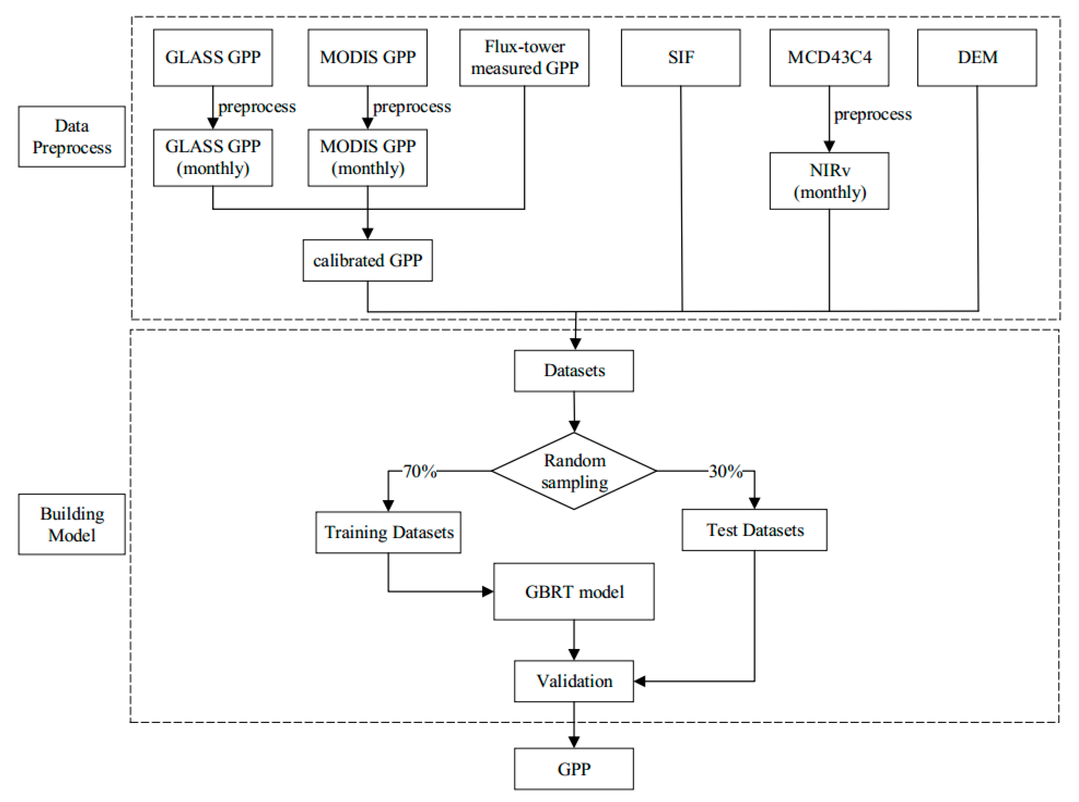
The schematic representation of the estimated GPP based on GOSIF SIF products and auxiliary data is shown in Figure 1.
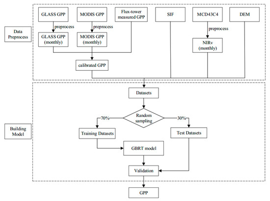
Figure 1.
Flowchart of the global GPP estimation from GOSIF SIF data.
The first step comprised data pre-processing. The data sources used in this study were not identical, and they featured different spatial and temporal resolutions. Therefore, to reduce the uncertainty caused by geographic location, all remote sensing data were converted to the same geographical projection (WGS84), and the data were resampled to the same spatial resolution as GOSIF (0.05°) using the bilinear interpolation method. In addition, to ensure the accuracy of machine learning methods during modeling, GPP ground observations should be used as the input variable in the training set of the machine learning model. However, the data volume derived from flux towers is small, the spatial scale of flux towers is small, the underlying ground surface is complex, and the vegetation types are diverse. As they are affected by spatial heterogeneity, it is difficult to directly apply the observations from the GPP flux towers to the regional scale. Therefore, we have calibrated the GPP products (MODIS GPP and GLASS GPP) through multiple linear regression methods, using flux observations from sites with different vegetation types. Thus, we have obtained new GPP datasets as “reference values” for the training set of the machine learning model.
The second step entailed building the model. In recent years, SIF and NIRv provide alternative approaches to estimate global GPP [45,70,73]. Meanwhile, precipitation and temperature are important for plant photosynthesis. Thus, we added SIF, DEM, land cover, NIRv, month, latitude, and longitude as explanatory variables. To ensure the robustness of the model, we randomly sampled the calibrated GPP datasets in 2001, 2004, 2007, 2010, and 2013, and added the explanatory variables. Then, the generated dataset was divided into a training dataset (70% of the generated dataset) and a validation dataset (30% of the generated dataset). Random forest (RF) is an integrated machine learning algorithm that integrates multiple weak classifiers (decision trees) [79]. Multivariate adaptive regression splines (MARS) is an automatic and adaptive nonparametric regression algorithm, which attempts to build a nonlinear regression model by fitting the weighted sum of multivariate spline basis functions [80]. The gradient boosting regression trees (GBRT) method proposed by Friedman is an iterative decision tree, which combines several weak classifiers in different proportions to form a strong classifier by additive model and forward distribution algorithm, and has been applied in remote sensing [81,82]. Light gradient boosting machine (LightTGBM) uses a decision tree-based learning algorithm that enables fast, efficient, parallel learning and large-scale data processing [83]. Long short-term memory (LSTM), a kind of neural network used for processing sequence data, is a special kind of recurrent neural network (RNN) [84]. In this study, global GPP estimation models were established using random forest (RF), MARS, GBRT, LightGBM, and LSTM algorithms using a training dataset. Subsequently, the validation dataset was used to validate these five models. The accuracies of models established by these algorithms were compared, and the optimal model and explanatory variables were selected to estimate the long-term global GPP.
Based on the five model results for the RF, MARS, GBRT, LightGBM, and LSTM algorithms, we compared two statistical indicators: coefficient of determination (R2) and root-mean-square error (RMSE) (see Appendix A for details). By comparing the accuracy of the model training dataset with the validation dataset and the efficiency of the model, we found that the GBRT model was more suitable for estimating global GPP based on GOSIF, and so we used this model to estimate global GPP from 2001 to 2017.
3. Results
3.1. Validation against Site GPP
We established linear correlations between the SIF-estimated GPP, MODIS GPP, and GLASS GPP (GPPSIF, GPPMOD, and GPPGLASS, respectively) and the flux tower GPP observations (GPPEC) for each vegetation type from 2001 to 2014, as shown in Table 1. For different vegetation types, GPPSIF (R2 = 0.16–0.78, RMSE = 1.50–4.72 g C·m−2·day−1, bias = –1.77–1.43 g C·m−2·day−1) performed well compared to GPPMODIS (R2 = 0.10–0.75, RMSE = 1.12–5.21 g C·m−2·day−1, bias = −2.14–0.54 g C·m−2·day−1) and GPPGLASS (R2 = 0.11–0.72, RMSE = 1.31–4.92 gC·m−2·day−1, bias = −1.14–2.23 g C·m−2·day−1). The poor performances of the different vegetation types may have been because of the small number of sites, or because of insufficient accuracy within the GPP products (e.g., the quality of the global land cover product). It is worth noting that the R2, RMSE, and the bias of wetlands (WET) did not perform well, meaning that more work is needed before the GPP of this vegetation type can be estimated using GOSIF datasets. The coefficients of determination of the three remote sensing products and GPPEC were small for evergreen broadleaf forests (EBF), savanna (SAV), and woody savannas (WSA), but were slightly higher for deciduous broadleaf forests (DBF), grasslands (GRA), and open shrublands (OSH). This indicates that the vegetation type had a great impact on the GPP estimations of remote sensing products. Referring to Table 1, the RMSE of the GPPMODIS–GPPEC model was the largest among the ten vegetation types. Overall, GPPSIF, GPPMOD, and GPPGLASS underestimated the GPP for croplands (CRO), DBF, evergreen needleleaf forests (ENF), mixed forests (MF), SAV, and WSA, whereas they overestimated GPP for OSH. More than half of the GPP values were underestimated by GPPMOD. MODIS GPP underestimated vegetation GPP, which has also been shown consistently in other studies [85,86]. For all sites, the correlations of GPPSIF–GPPEC, GPPMODIS–GPPEC, and GPPGLASS–GPPEC were similar, but GPPSIF–GPPEC had the lowest RMSE and bias. To some extent, GOSIF demonstrated the ability to estimate GPP, and SIF outperformed the LUE model with regards to estimating GPP. The poor performances of GPPMODIS and GPPGLASS may have been because MODIS and GLASS used the LUE model to calculate GPP. is a key parameter within the LUE model, but it exhibits great variability within a single biological community. In the LUE model, is often set as a fixed parameter according to a specific vegetation type, leading to great uncertainty in the estimation of GPP. Moreover, the vegetation index is not sensitive to changes in plant photosynthetic status when vegetation is under stress (e.g., due to temperature extremes or limited water). This could also lead to inaccuracies in the model. In contrast, SIF is very sensitive to plant growth status.

Table 1.
Comparisons of R2, RMSE, and bias between GPPSIF, GPPMODIS, GPPGLASS, and GPPEC for different vegetation types for the period 2001 to 2014. CRO: croplands, DBF: deciduous broadleaf forests, EBF: evergreen broadleaf forests, ENF: evergreen needleleaf forests, GRA: grasslands, MF: mixed forests, OSH: open shrublands, SAV: savannas, WET: wetland, and WSA: woody savannas.
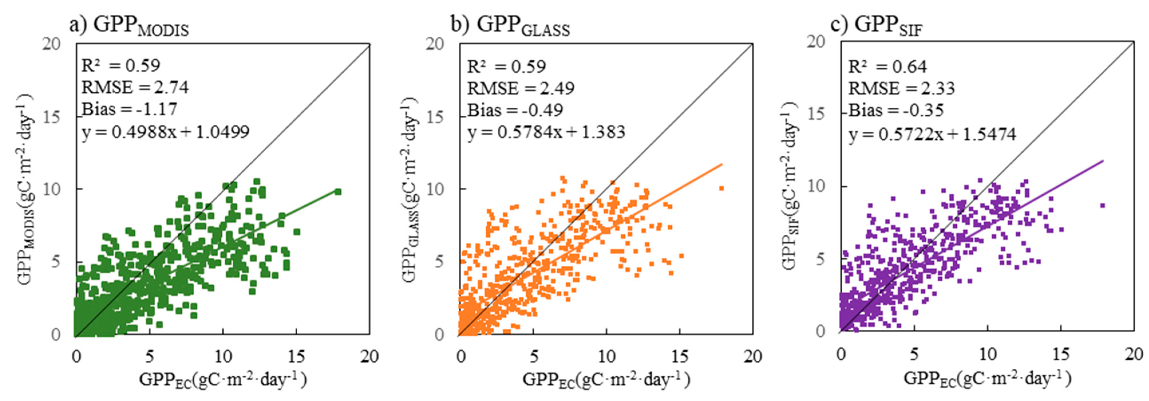
Scatter plots between GPPMOD and GPPEC, and scatter plots between GPPGLASS and GPPEC, and scatter plots between GPPSIF and GPPEC were analyzed in 2014, as shown in Figure 2. R2 between GPPMOD and GPPEC was 0.59, RMSE was 2.74 g C·m−2·day−1, and Bias was –1.17 g C·m−2·day−1. As for the GLASS GPP, R2 was 0.59, RMSE was 2.49 g C·m−2·day−1, and Bias was –0.49 g C·m−2·day−1. R2 between GPPSIF and GPPEC could be as high as 0.64, RMSE was 2.33 g C·m−2·day−1, and Bias was –0.35 g C·m−2·day−1. We found that RMSEs of GPPGLASS–GPPEC and GPPSIF–GPPEC in 2014 was marginally smaller than RMSE of GPPMOD–GPPEC in 2014. Therefore, we found that GPPSIF achieved the highest precision in 2014.

Figure 2.
Evaluation of GPPMOD, GPPGLASS and GPPSIF against FLUXNET GPP in 2014.
3.2. Spatial Patterns of Estimated GPP
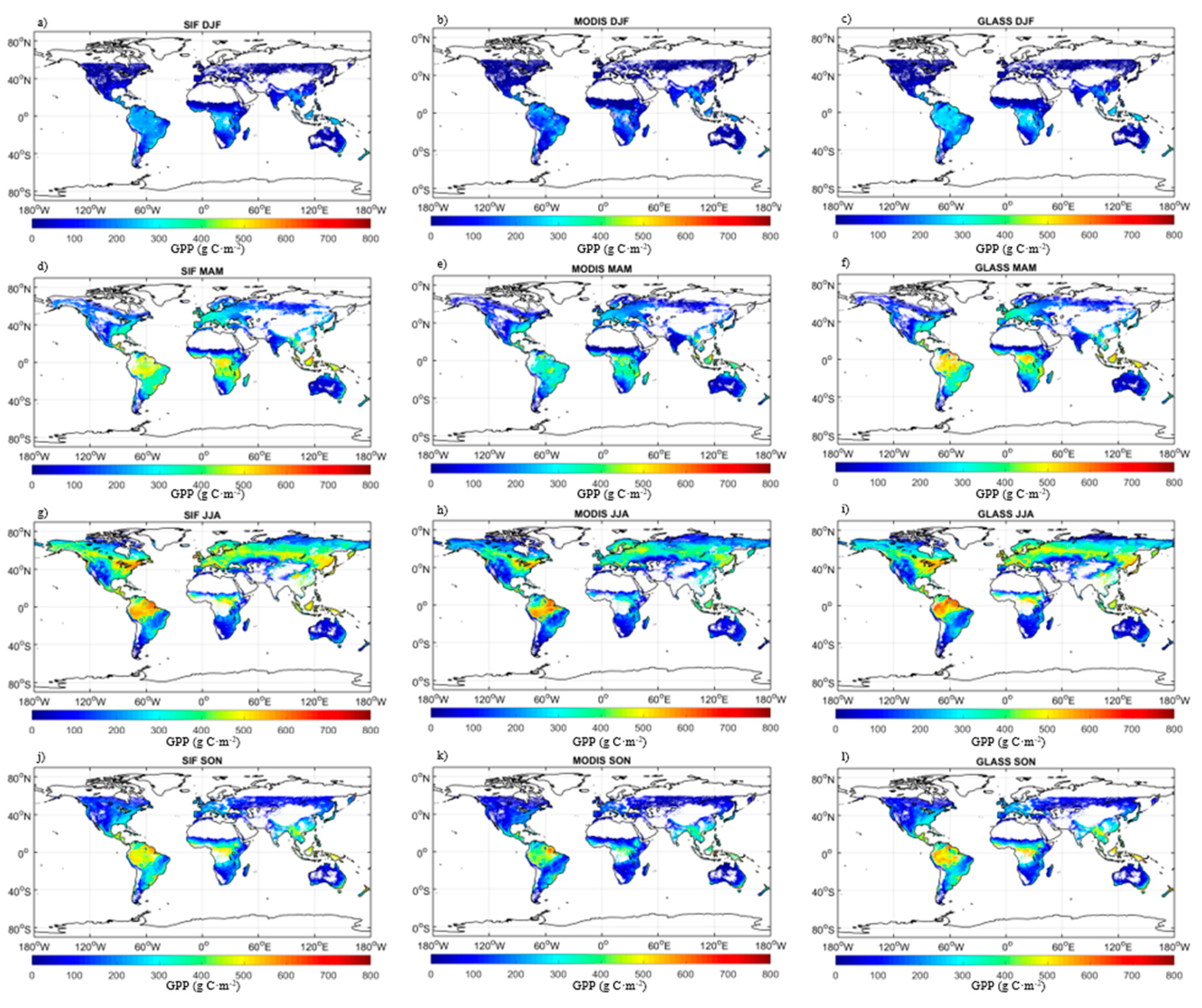
We generated 0.05° GPPSIF data from 2001 to 2017, and maps of global GPP in 2014, as shown in Figure 3. Maps of other years are given in Appendix B. The absence of input data at high latitudes led us to mask the seasonal results at high latitudes when comparing the spatial patterns and seasonal variations of the three products. Compared with GPPMOD and GPPGLASS, our GPPSIF exhibited reasonable spatial and seasonal variation on a global scale. Comparing the three GPP products for different seasons in 2014 revealed that GPPSIF exhibited a high level of agreement with GPPGLASS and a low level of agreement with the GPPMOD. The seasonal variation observed in GPPMOD was not as great as that in the other two GPP products. In addition, GPPGLASS and GPPSIF exhibited greater seasonal changes, especially in tropical regions. GPPMOD was visually different from the other two products in tropical regions.
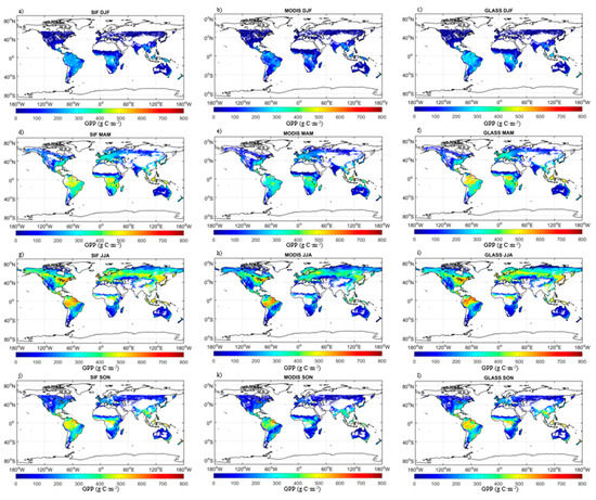
Figure 3.
Spatial patterns of global GPP in different seasons of 2014: (a) GPPSIF in December, January, and February (DJF); (b) GPPMODIS in DJF; (c) GPPGLASS in DJF; (d) GPPSIF in March, April and May (MAM); (e) GPPMODIS in MAM; (f) GPPGLASS in MAM; (g) GPPSIF in June, July, and August (JJA); (h) GPPMODIS in JJA; (i) GPPGLASS in JJA; (j) GPPSIF in September, October, and November (SON); (k) GPPMODIS in SON; (l) GPPGLASS in SON.
In December, January, and February (DJF), global GPP was mainly concentrated in the range of 0 to 300 g C·m−2, and the highest GPP (GPP > 200 g C·m−2) were found in humid tropical areas such as Amazonia, Central Africa, and Southeast Asia. In the Northern Hemisphere, GPP above 30° was generally below 100 g C·m−2. In March, April, and May (MAM), global GPP was mainly between 0and 500 g C·m−2. The GPP values of North America, Asia, and Europe ranged between 100 and 300 g C·m−2, whereas most of Australia was below 100 g C·m−2. The highest GPP (GPP > 300 g C·m−2) was found in Amazonia, Central Africa, and Southeast Asia. In June, July, and August (JJA), global GPP was mainly about 400 g C·m−2. The highest GPP were mainly between 500 and 600 g C·m−2, and was found in the Amazon. The GPP of North America, Europe, and Asia were mainly between 300 and 500 g C·m−2. Within this, GPP was lower in some high-altitude regions, such as the Iranian plateau, the Mongolian plateau, and the Rocky Mountains. In September, October, and November (SON), high GPP values ranged between 400 and 600 g C·m−2, and were distributed in the Amazon and Southeast Asia. Across the rest of the world, GPP was mainly between 100 and 300 g C·m−2 at this time. The seasonal pattern of global GPP revealed that the regions with the highest GPP were mainly in humid tropical areas such as the Amazon, Central Africa, and Southeast Asia, where both the temperature and moisture requirements for photosynthesis are adequately satisfied. Vegetation productivity in temperate regions was at an intermediate level, and vegetation productivity in cold and higher altitude regions was the lowest because temperature and or precipitation in these regions were limited.
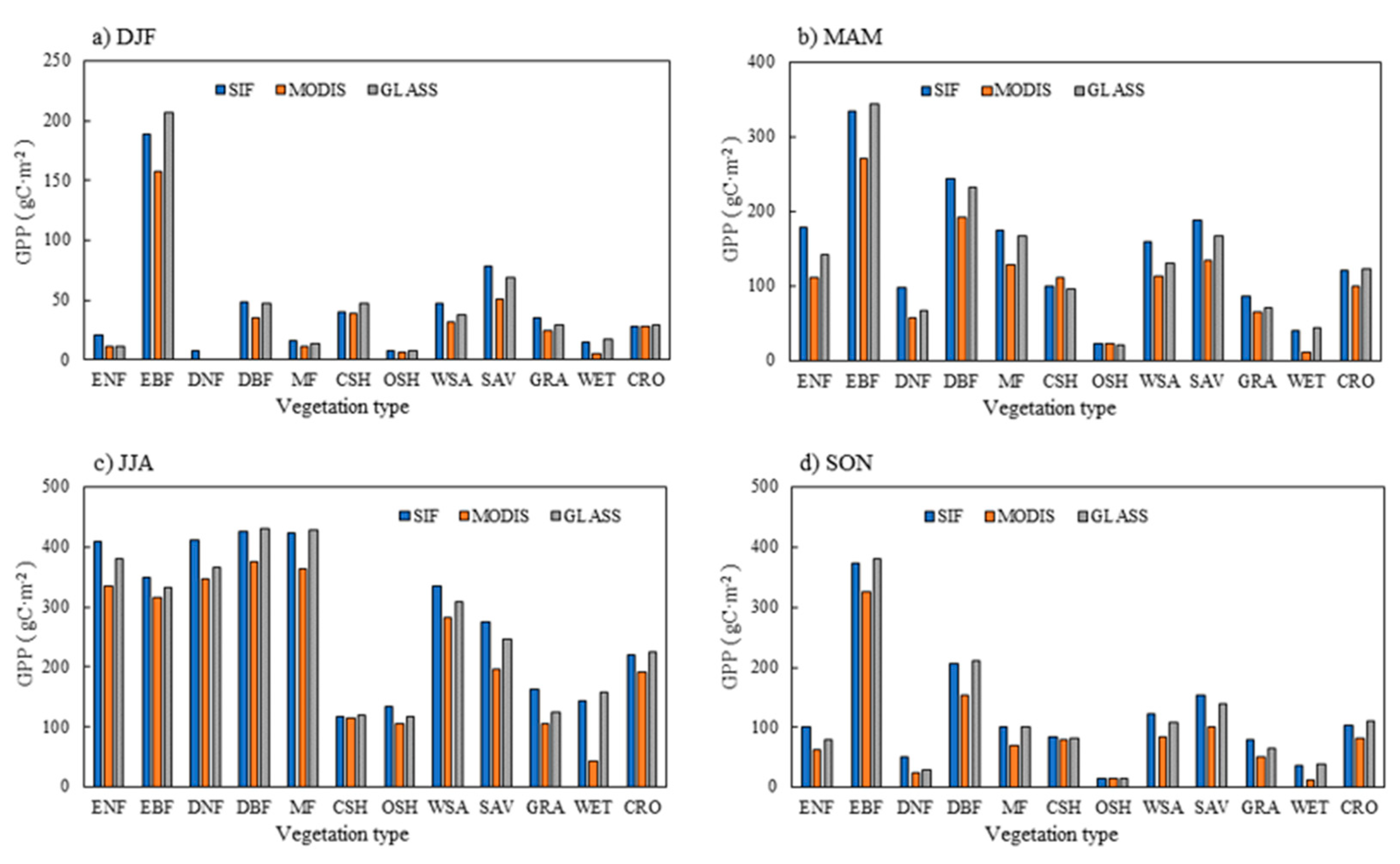
The GPP of different vegetation coverage types in each season in 2014 is shown in Figure 4 (note missing high latitude values). The GPP was highest in JJA, which was also related to the amount of data (GOSIF had fewer missing values at high latitudes for JJA). EBF had high GPP throughout the year, whereas GPP was always low for CSH, OSH, and WET. Comparing the statistics of the three GPP products for different vegetation coverage types, the barplot from the four seasons shows that the GPP of MODIS was low compared to the other two GPP products. In DJF, the EBF GPP reached as high as 189.30 g C·m−2(GPPSIF), 157.89 g C·m−2 (GPPMODIS), and 206.72 g C·m−2(GPPGLASS), with a difference of up to 48.83 g C·m−2 between the three products. Except for ENF, GPPMODIS was the lowest among the three products across different vegetation coverage types. The GPPSIF, GPPMODIS, and GPPGLASS of CRO were all almost equal (28.48 g C·m−2, 27.60 g C·m−2, and 29.49 g C·m−2, respectively). In MAM, the GPP of ENF, EBF, DBF, MF, SAV, and WSA all exceeded 100 g C·m−2. GPPGLASS was also higher than GPPSIF regarding EBF while the GPP of MODIS was higher than the other two GPP products in CSH and OSH. The GPPSIF, GPPMODIS, and GPPGLASS of OSH were similar (22.00 g C·m−2, 22.57 g C·m−2, and 19.97 g C·m−2, respectively). During JJA, the GPP of CSH, OSH, GRA, and WET did not exceed 150 g C·m−2. Among the different vegetation coverage types, the GPPSIF and GPPGLASS were all almost equal in EBF, DBF, MF, CSH, and CRO. For EBF, the differences between the three products were the smallest in a year. The GPPSIF, GPPMODIS, and GPPGLASS of CSH were all almost equal (118.07 g C·m−2, 114.89 g C·m−2, and 118.88 g C·m−2, respectively). During SON, the GPP of each vegetation coverage type decreased to a certain extent, compared with the previous season. The GPP of ENF, DNF, CSH, OSH, and WET were almost below 100 gc·m−2. The GPPSIF and GPPGLASS of EBF, DBF, MF, CSH, OSH, and WET were all very similar, which was in clear contrast with GPPMODIS. For CSH and OSH, GPPSIF, GPPMODIS, and GPPGLASS were almost equal.
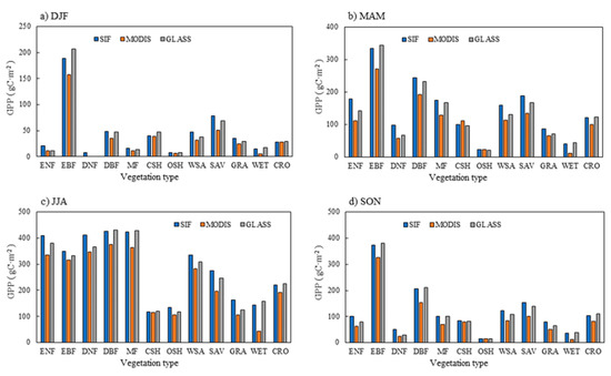
Figure 4.
Global GPP for all vegetation coverage types in GPPSIF, GPPMODIS and GPPGLASS in different seasons in 2014.
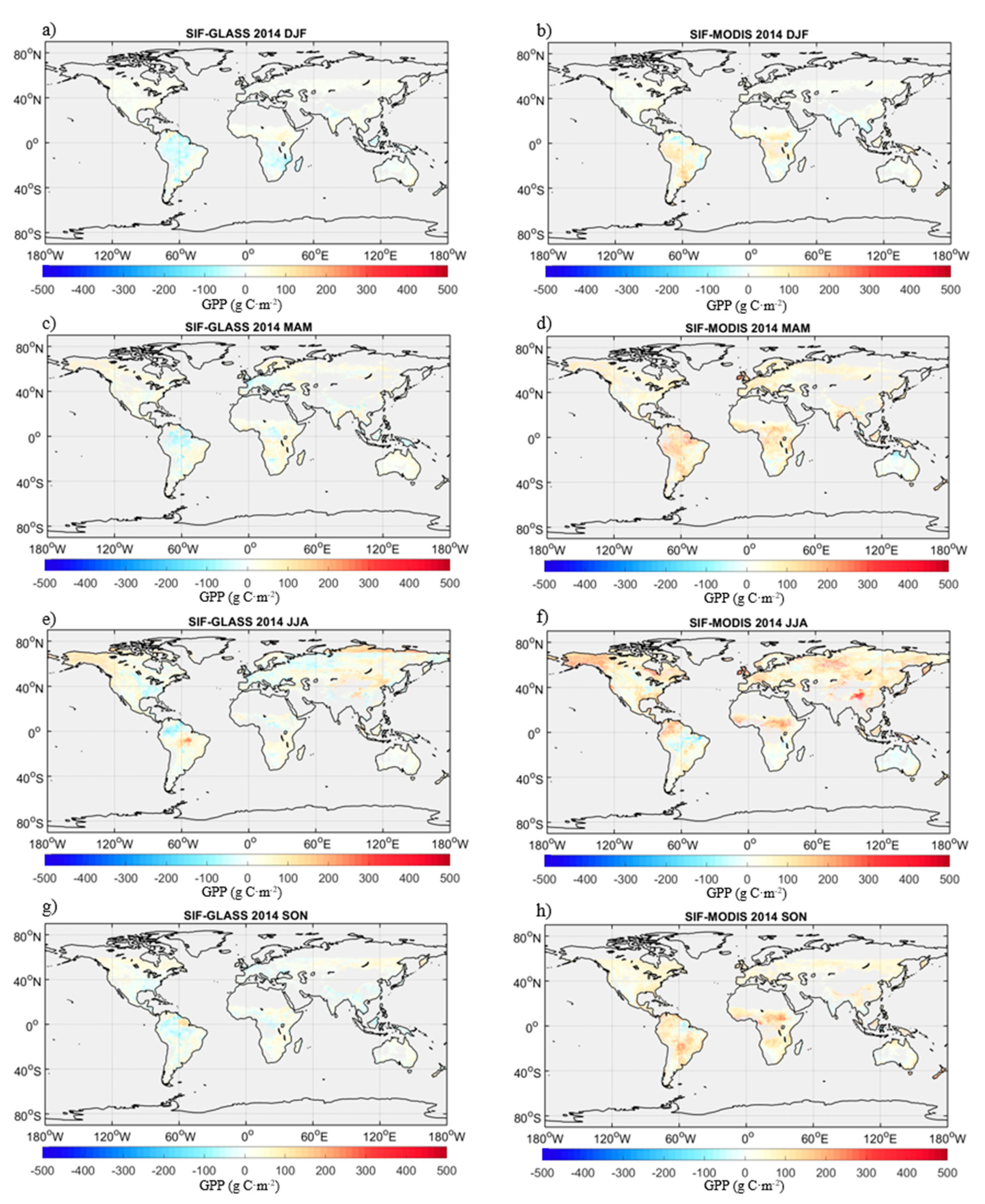
The differences between GPPSIF and those of the other products are shown in Figure 5. During DJF, the differences between GPPSIF and GPPMODIS were mainly between –100 and 200 g C·m−2, with differences ranged between 0 and 100 g C·m−2 in Europe and Asia, ranged between –100 and 0 g C·m−2 in Southern Asia and Southeast Asia, ranged between 100 and 200 g C·m−2 in Central Africa and the Amazon. The differences between the GPPSIF and GPPGLASS were mainly between –100 and 100 g C·m−2. In tropical regions such as Southeast Asia, Central Africa, and the Amazon, the differences were mainly between –100 and 0 g C·m−2. In MAM, the differences between GPPSIF and GPPMODIS were mainly between 0 and 100 g C·m−2, with a few regions in the Amazon, Central Africa, and Europe having differences ranged between 100 and 200 g C·m−2; in the northern part of Australia, it reached –100 g C·m−2. The differences between GPPSIF and GPPGLASS were mainly between 0 and 100 g C·m−2, with some parts of the Amazon, Central Africa, and Europe exhibiting differences around –100 g C·m−2. In JJA, the differences between GPPSIF and GPPMODIS were mainly between –100 and 200 g C·m−2, with differences between 100 and 200 g C·m−2 in the equatorial tropics. Some regions in Central Africa exhibited differences as high as 200 to 300 g C·m−2. The differences between GPPSIF and GPPGLASS were mainly between –100 and 200 g C·m−2; Eastern Europe and North Asia exhibited differences in the range of 100 to 200 g C·m−2, with one part of the central Amazon reaching a difference of 200 g C·m−2. In SON, the difference between GPPSIF and GPPMODIS was mainly in the range of –100 to 200 g C·m−2. The larger differences were mostly located near the equator. The differences between the GPPSIF and GPPGLASS were mainly between –100 and 100 g C·m−2. It is noteworthy that some of the differences around the equator reached 200 g C·m−2, especially in the Guiana Plateau in northern South America. It is not difficult to determine that many of the large differences were concentrated in tropical regions and regions with high altitudes. In humid tropical regions at lower latitudes, where the temperature and humidity requirements for photosynthesis are adequately satisfied, the vegetation coverage types are complex and unevenly distributed, resulting in large differences in GPP and inaccurate predictions. Areas at higher latitudes or altitudes, where there are limited temperature and precipitation and so photosynthesis is limited, have homogeneous vegetation distributions and are therefore less complex than areas in the tropics. As a result, the GPP of these areas is lower overall, and the differences in GPP between various vegetation types are small. Therefore, predictions in these areas have appeared to be more accurate.
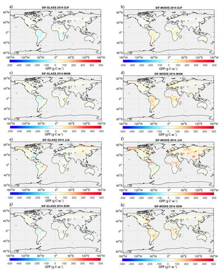
Figure 5.
Differences in spatial patterns of global GPP in different seasons in 2014: (a) difference between GPPSIF and GPPGLASS in DJF; (b) difference between GPPSIF and GPPMODIS in DJF; (c) difference between GPPSIF and GPPGLASS in MAM; (d) difference between GPPSIF and GPPMODIS in MAM; (e) difference between GPPSIF and GPPGLASS in JJA; (f) difference between GPPSIF and GPPMODIS in JJA; (g) difference between GPPSIF and GPPGLASS in SON; (h) difference between GPPSIF and GPPMODIS in SON.
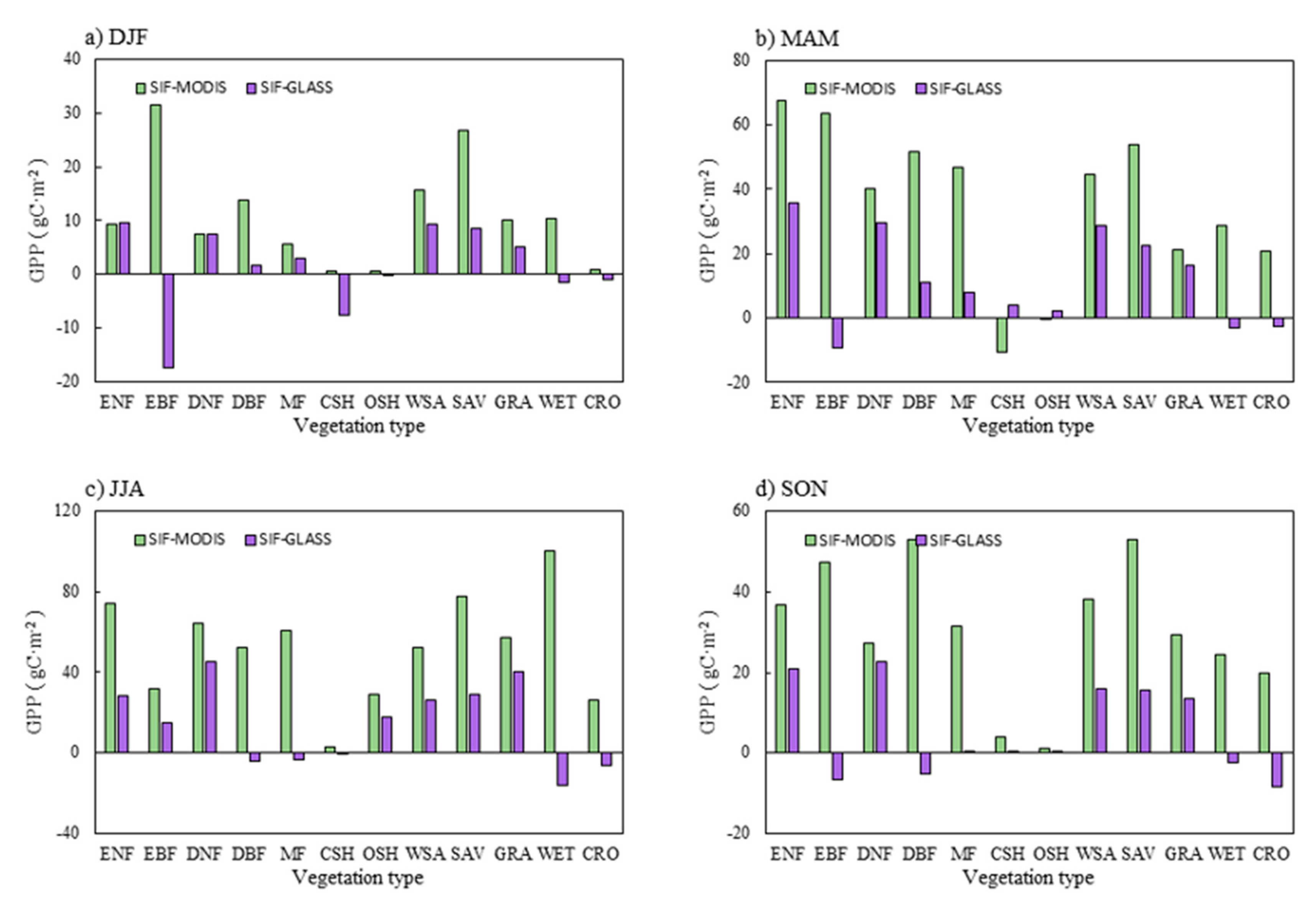
The differences between the three GPP products for different vegetation coverage types in each season in 2014 are shown in Figure 6. Regardless of the season, the GPPSIF was essentially higher than those of the other two products. The GPP productivity of the three products differed, especially for EBF, DBF, WSA, SAV, WET, and CRO. GPPGLASS is higher than the other two GPP products for DJF, MAM, and SON for EBF. GPPGLASS is greater than that of the other two products for CRO and WET. GPPMODIS is always lower than GPP except for CSH in MAM. CSH and OSH had the smallest differences because of their low global distribution.
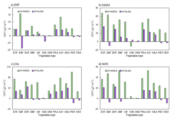
Figure 6.
Differences in global GPP for all vegetation coverage types in different seasons in 2014 (green represents the difference between GPPSIF and GPPMODIS, purple represents the difference between GPPSIF and GPPGLASS).
4. Discussion
4.1. Relative Importance of Variables
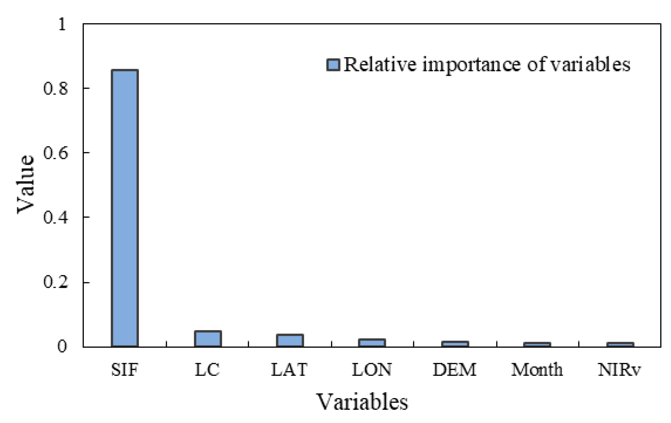
In estimating global GPP, the variables used in the model included monthly SIF, Land cover, latitude, longitude, DEM, month, and NIRv. We discussed the relative importance of variables and the results as shown in Figure 7. Generally, SIF was the most important variable in estimating global GPP. The other variables contributed less in estimating global GPP in this study. This conclusion fully reflects the relationship between SIF and GPP, which is strongly consistent with most research results [45,48,53,54]. Other variables used in this study, such as latitude, longitude, DEM, month, etc., reflect precipitation and temperature information and are important for plant photosynthesis. SIF and NIRv provide alternative approaches to estimate global GPP [45,70,73], but as shown in Figure 7, SIF was far more important than NIRv. The advantages and differences of SIF and NIRV estimation of GPP need to be further studied. Although the contribution of these variables to the estimation of GPP is small, the best estimates can only be obtained by using all GPP-related variables.
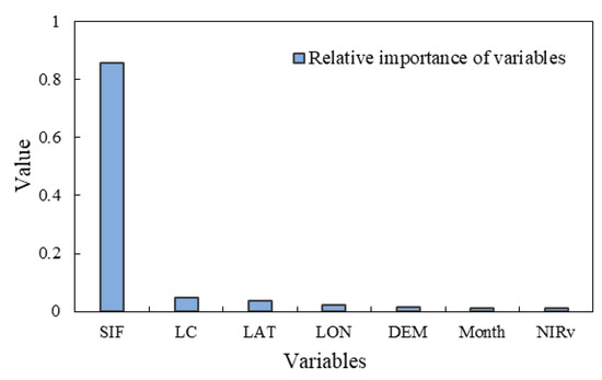
Figure 7.
The relative importance of variables to the GPP estimation GBRT model built from the training dataset.
4.2. Limitations of the Current Study
The results of this study reveal that the GOSIF dataset has great potential for estimating GPP for different vegetation coverage types. Our method requires fewer input variables and has higher computational efficiency than other satellite GPP estimation methods. Satellite-based SIF data provide a unique opportunity for more accurate, near real-time GPP mapping in the future.
However, its suitability varies somewhat. One of the main reasons for this is that significant amounts of flux tower data are not available to the public, and the available data are not evenly distributed across the globe. Consequently, there are huge challenges for using GPPEC to validate SIF-estimated GPP or other GPP products on a global scale. In addition, inaccurate GPPEC observations can also cause errors. To some extent, GPPEC observations obtained by flux towers can simply be considered as “reference values”. However, different flux towers have different qualities [85]. Moreover, in this study, we assumed that the vegetation coverage types around the flux towers were homogeneous and uneven. This assumption does not hold consistently. In general, we believe that the smaller the pixel corresponding to the product at the location of the flux tower, the more representative the reference value of the pixel likely is. Here, we used site data to calibrate the GPP products with a spatial resolution of 500 m, and then resampled to 0.05°; this will affect the accuracy of the results. Above all, the input variables of the model training set used in this study also introduced certain uncertainties.
The SIF signal exhibited a strong relationship with GPP, which can be explained mechanistically as follows. Based on the LUE model, GPP can be expressed as Equation (1).
SIF can be similarly conceptualized as a byproduct of photosynthesis, which can be expressed as [34]:
where is the spectral wavelength, is the fluorescence quantum yield (i.e., the rate at which a plant absorbs photosynthetically effective radiation and re-emits fluorescence at the wavelength ), and is the ratio at which fluorescence emitted by chloroplasts can escape out of the canopy. Equations (1) and (3) can be combined to describe the theoretical formulation of the GPP-SIF relationship as follows:
For the same vegetation type, remains relatively constant, and if the ratio is constant then should be a good constraint on the photosynthetic rate, regardless of changes in FPAR, PAR, or environmental stresses. Thus, for this study, the land cover type determined to some extent, whereas NIRv was used as an approximation of the canopy-escaping probability of emitted SIF.
Over the years, many researches have demonstrated that SIF and GPP have a strong linear relationship compared with the traditional vegetation index [9,45,48]. However, GPP estimates by SIF have been limited by the spatial resolution of the satellite spatial resolution. GOSIF(0.05°) offers a finer spatial resolution than other SIF products (e.g., 0.5°), providing an unprecedented opportunity to explore the estimation of GPP on an ecosystem or global scale. However, the spatial resolution of GOSIF is currently far from sufficient. To date, there is no global high-precision SIF remote sensing product for estimating GPP on a large regional scale. Here, MODIS datasets, such as the Enhanced Vegetation Index (EVI) and PAR, were used to calculate GOSIF data, and then data were resampled to 0.05°, which would have caused errors in the predictions. In addition to the uncertainty caused by additional model inputs, the quality of OCO-2 SIF also represented a source of uncertainty for GOSIF in this study. Currently, there are no satellites dedicated to SIF observation. Hence, it is necessary to obtain more accurate SIF datasets. The greatest limitation of the current research is that the spatial resolution and temporal resolution of SIF data are too low to reflect the greatest advantage of SIF estimation of GPP: real-time estimation [85]. Additionally, the linear relationship between SIF and GPP for different vegetation types is different on different time scales [56,87].
Further to the above-stated issues, other input variables in the model and the number of training samples will also have an impact on the results of this study. We argue that the uncertainty of GPP can be estimated by remote sensing data across vegetation coverage types. The accuracy of the vegetation coverage type data has a significant impact on the accuracy of the LUE model, which is one of the advantages of using SIF to estimate GPP. But in this study, we also used the land cover types data [17]. Hence, producing accurate estimates of predictions of land cover types and NIRv are further issues that urgently need to be addressed when estimating GPP.
5. Conclusions
Most current research into sun-induced chlorophyll fluorescence (SIF)-estimated Gross primary production (GPP) focuses on flux towers and at small regional scales. GPP can be obtained based on the relationship between SIF and GPP, but there are still complex basic physiological processes that need to be constrained. Therefore, it is difficult to quantitatively evaluate the factors that affect the relationship between SIF and GPP.
In this study, global GPP was estimated from GOSIF SIF data using the gradient boosting regression trees (GBRT) model at a spatial resolution of 0.05°. In this model, we also used land cover, DEM, NIRv, and other data as input variables while SIF was far more important than other variables. This is a new method for estimating GPP using SIF on a global scale. Subsequently, we evaluated the performance of three GPP products GPPSIF, GPPMODIS, and GPPGLASS, when estimating GPP from flux towers and for different vegetation types. Our results show that SIF can estimate global GPP very well, and the GPP estimated based on GOSIF is similar to the results of that derived from FLUXNET sites (R2 = 0.58, RMSE = 2.74 g C·m−2, bias = −0.34 g C·m−2). Furthermore, the GPP that we estimated using GOSIF demonstrated reasonable spatial and seasonal changes on a global scale. Although we have revealed that it is possible to estimate GPP from SIF at the satellite scale, challenges remain in estimating GPP directly from SIF at the regional or global scale. In the future, the accuracy of estimations of GPP using SIF could be improved by obtaining higher-quality SIF remote sensing datasets.
Author Contributions
Y.B. and S.L. designed the experiment. Y.B. collected and preprocessed the data. Y.B., S.L. and W.Y. performed the experiment and conducted the analysis. All authors have read and agreed to the published version of the manuscript.
Funding
This study was partially funded by the National Key Research and Development Program of China (no. 2016YFA0600101).
Data Availability Statement
All data used in this study were from open access satellite products or published field work cited in this article.
Conflicts of Interest
The authors declare no conflict of interest.
Appendix A
Results of Five Algorithms on Validation Datasets
In this study, we used random forest (RF), multivariate adaptive regression splines (MARS), gradient boosting regression trees (GBRT), light gradient boosting machine (LightGBM), and long short-term memory (LSTM) algorithms to build GPP estimation models. In addition, the testing dataset was a randomly selected 30% of the generated dataset used to validate these models. Based on the training and testing results for the five algorithms. The validation results for the five models are given in Table A1. We determined the optimal models by comparing their respective R2 and root mean square error (RMSE) values. Based on a comparison of results, we found that the GBRT model was better than the other four models in this study. The R2 values based on the GBRT model were higher than the other four models while the RMSE achieved by the GBRT model was also lower than others.

Table A1.
The validation results for five models.
Table A1.
The validation results for five models.
| Methods | Test | |
|---|---|---|
| R2 | RMSE (g C·m−2) | |
| RF | 0.95 | 0.72 |
| MARS | 0.87 | 1.19 |
| GBRT | 0.98 | 0.59 |
| LightGBM | 0.96 | 0.62 |
| LSTM | 0.92 | 0.92 |
Appendix B
Spatial Patterns of Global GPPSIF in Different Seasons
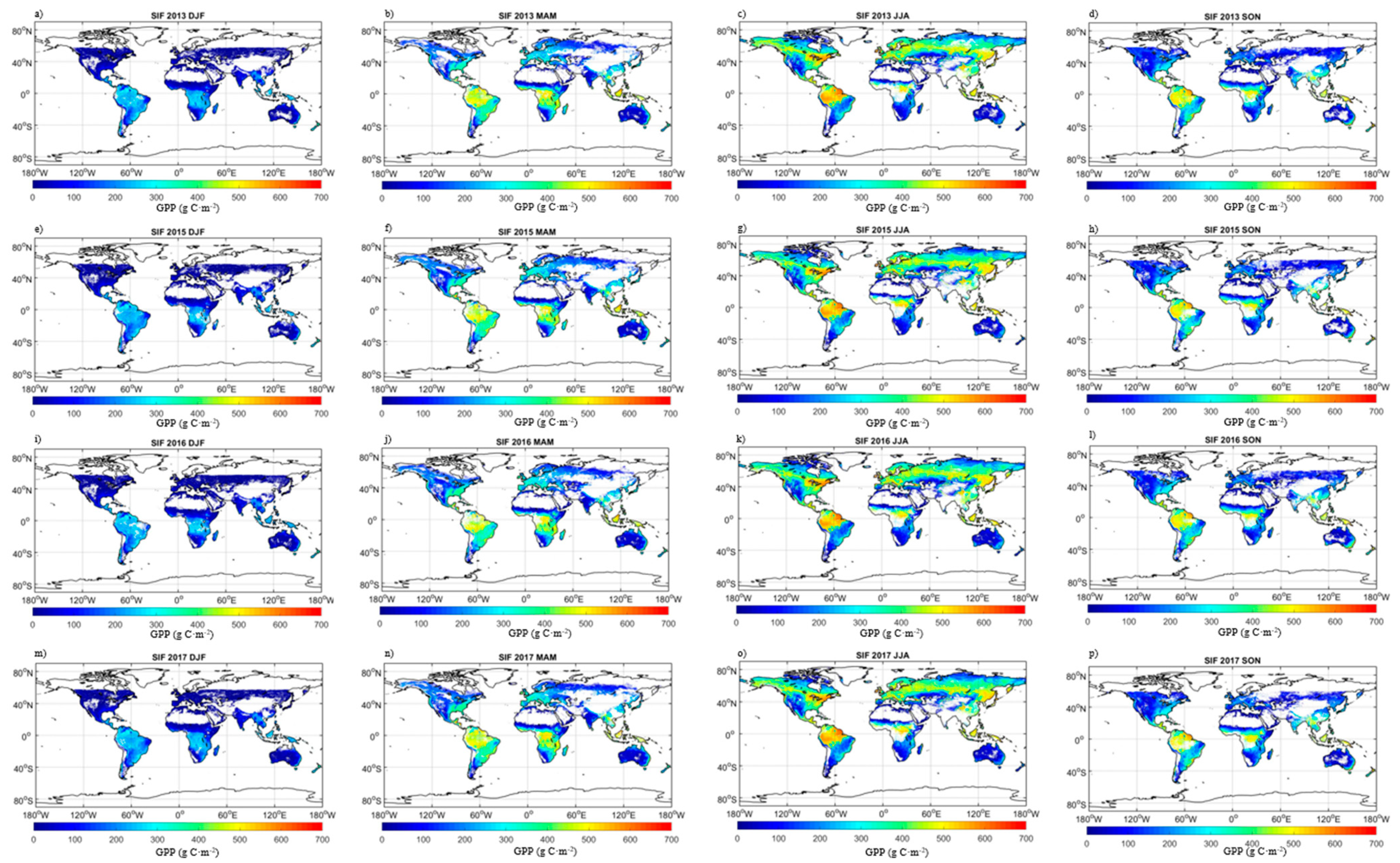
We mapped global GPPSIF for the period 2001–2017 (except 2014), as shown in Figure A1, Figure A2, Figure A3 and Figure A4.
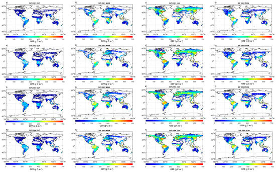
Figure A1.
Spatial patterns of global GPP in different seasons: (a) GPPSIF in DJF of 2001; (b) GPPSIF in MAM of 2001; (c) GPPSIF in JJA of 2001; (d) GPPSIF in SON of 2001; (e) GPPSIF in DJF of 2002; (f) GPPSIF in MAM of 2002; (g) GPPSIF in JJA of 2002; (h) GPPSIF in SON of 2002; (i) GPPSIF in DJF of 2003; (j) GPPSIF in MAM of 2003; (k) GPPSIF in JJA of 2003; (l) GPPSIF in SON of 2003; (m) GPPSIF in DJF of 2004; (n) GPPSIF in MAM of 2004; (o) GPPSIF in JJA of 2004; (p) GPPSIF in SON of 2004.
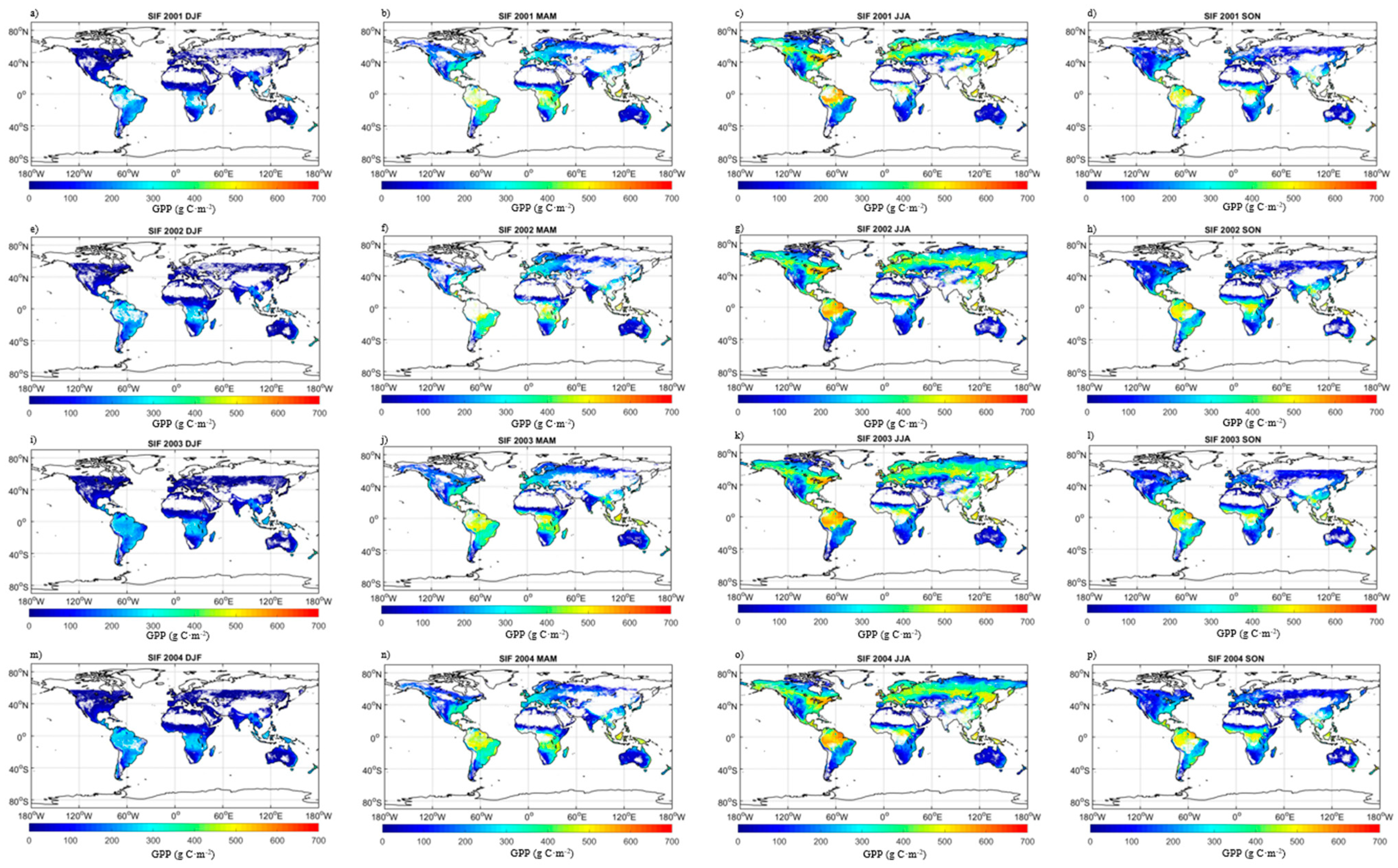
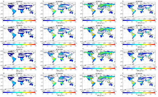
Figure A2.
Spatial patterns of global GPP in different seasons: (a) GPPSIF in DJF of 2005; (b) GPPSIF in MAM of 2005; (c) GPPSIF in JJA of 2005; (d) GPPSIF in SON of 2005; (e) GPPSIF in DJF of 2006; (f) GPPSIF in MAM of 2006; (g) GPPSIF in JJA of 2006; (h) GPPSIF in SON of 2006; (i) GPPSIF in DJF of 2007; (j) GPPSIF in MAM of 2007; (k) GPPSIF in JJA of 2007; (l) GPPSIF in SON of 2007; (m) GPPSIF in DJF of 2008; (n) GPPSIF in MAM of 2008; (o) GPPSIF in JJA of 2008; (p) GPPSIF in SON of 2008.
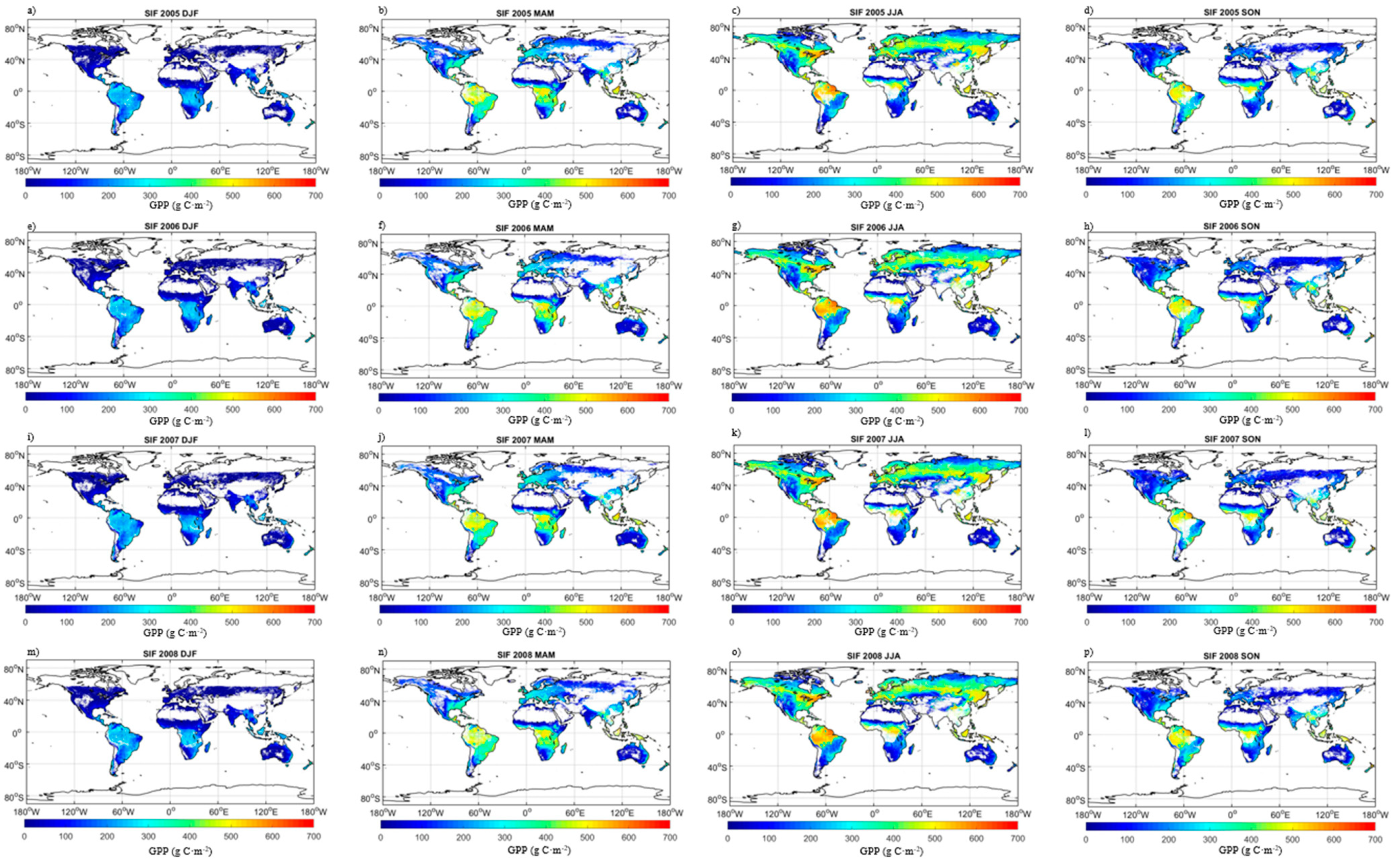
Figure A3.
Spatial patterns of global GPP in different seasons: (a) GPPSIF in DJF of 2009; (b) GPPSIF in MAM of 2009; (c) GPPSIF in JJA of 2009; (d) GPPSIF in SON of 2009; (e) GPPSIF in DJF of 2010; (f) GPPSIF in MAM of 2010; (g) GPPSIF in JJA of 2010; (h) GPPSIF in SON of 2010; (i) GPPSIF in DJF of 2011; (j) GPPSIF in MAM of 2011; (k) GPPSIF in JJA of 2011; (l) GPPSIF in SON of 2011; (m) GPPSIF in DJF of 2012; (n) GPPSIF in MAM of 2012; (o) GPPSIF in JJA of 2012; (p) GPPSIF in SON of 2012.
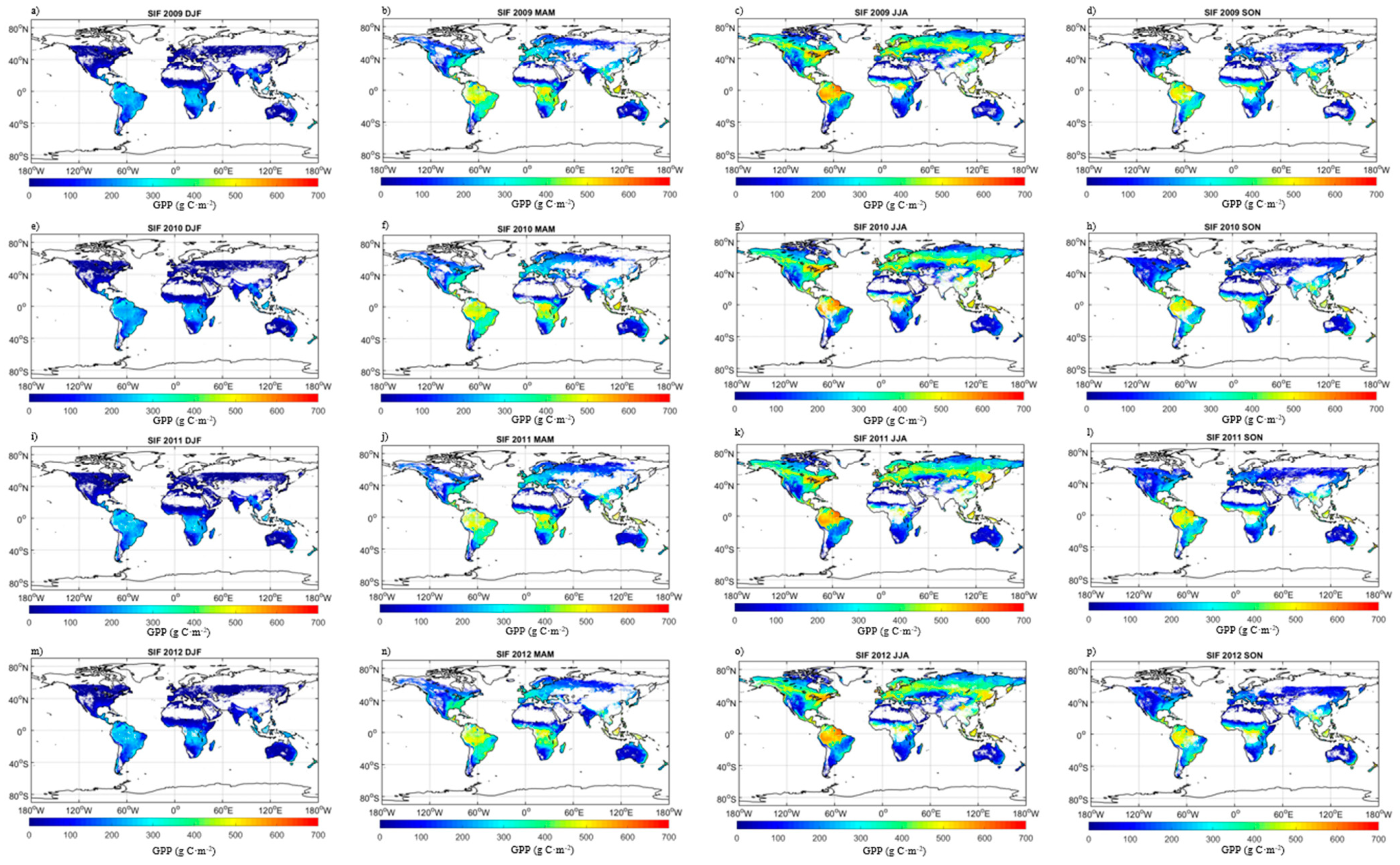
Figure A4.
Spatial patterns of global GPP in different seasons: (a) GPPSIF in DJF of 2013; (b) GPPSIF in MAM of 2013; (c) GPPSIF in JJA of 2013; (d) GPPSIF in SON of 2013; (e) GPPSIF in DJF of 2015; (f) GPPSIF in MAM of 2015; (g) GPPSIF in JJA of 2015; (h) GPPSIF in SON of 2015; (i) GPPSIF in DJF of 2016; (j) GPPSIF in MAM of 2016; (k) GPPSIF in JJA of 2016; (l) GPPSIF in SON of 2016; (m) GPPSIF in DJF of 2017; (n) GPPSIF in MAM of 2017; (o) GPPSIF in JJA of 2017; (p) GPPSIF in SON of 2017.
References
- Karlson, R.H.; Cornell, H.V.; Hughes, T.P. Coral communities are regionally enriched along an oceanic biodiversity gradient. Nature 2004, 429, 867–870. [Google Scholar] [CrossRef]
- Krausmann, F.; Erb, K.H.; Gingrich, S.; Haberl, H.; Bondeau, A.; Gaube, V.; Lauk, C.; Plutzar, C.; Searchinger, T.D. Global human appropriation of net primary production doubled in the 20th century. Proc. Natl. Acad. Sci. USA 2013, 110, 10324–10329. [Google Scholar] [CrossRef]
- Migliavacca, M.; Perez-Priego, O.; Rossini, M.; El-Madany, T.S.; Moreno, G.; van der Tol, C.; Rascher, U.; Berninger, A.; Bessenbacher, V.; Burkart, A.; et al. Plant functional traits and canopy structure control the relationship between photosynthetic CO2 uptake and far-red sun-induced fluorescence in a Mediterranean grassland under different nutrient availability. New Phytol. 2017, 214, 1078–1091. [Google Scholar] [CrossRef] [PubMed]
- Beer, C.; Reichstein, M.; Tomelleri, E.; Ciais, P.; Jung, M.; Carvalhais, N.; Rödenbeck, C.; Arain, M.A.; Baldocchi, D.; Bonan, G.B. Terrestrial gross carbon dioxide uptake: Global distribution and covariation with climate. Science 2010, 329, 834–838. [Google Scholar] [CrossRef]
- Yu, G.R.; Zhu, X.J.; Fu, Y.L.; He, H.L.; Wang, Q.F.; Wen, X.F.; Li, X.R.; Zhang, L.M.; Zhang, L.; Su, W.; et al. Spatial patterns and climate drivers of carbon fluxes in terrestrial ecosystems of China. Glob. Chang. Biol. 2013, 19, 798–810. [Google Scholar] [CrossRef]
- Damm, A.; Elbers, J.; Erler, A.; Gioli, B.; Hamdi, K.; Hutjes, R.; Kosvancova, M.; Meroni, M.; Miglietta, F.; Moersch, A. Remote sensing of sun-induced fluorescence to improve modeling of diurnal courses of gross primary production (GPP). Glob. Chang. Biol. 2010, 16, 171–186. [Google Scholar] [CrossRef]
- Damm, A.; Guanter, L.; Paul-Limoges, E.; van der Tol, C.; Hueni, A.; Buchmann, N.; Eugster, W.; Ammann, C.; Schaepman, M.E. Far-red sun-induced chlorophyll fluorescence shows ecosystem-specific relationships to gross primary production: An assessment based on observational and modeling approaches. Remote Sens. Environ. 2015, 166, 91–105. [Google Scholar] [CrossRef]
- Joiner, J.; Yoshida, Y.; Zhang, Y.; Duveiller, G.; Jung, M.; Lyapustin, A.; Wang, Y.; Tucker, C.J. Estimation of terrestrial global gross primary production (GPP) with satellite data-driven models and eddy covariance flux data. Remote Sens. 2018, 10, 1346. [Google Scholar] [CrossRef]
- Li, X.; Xiao, J.; He, B.; Altaf Arain, M.; Beringer, J.; Desai, A.R.; Emmel, C.; Hollinger, D.Y.; Krasnova, A.; Mammarella, I.; et al. Solar-induced chlorophyll fluorescence is strongly correlated with terrestrial photosynthesis for a wide variety of biomes: First global analysis based on OCO-2 and flux tower observations. Glob. Chang. Biol. 2018, 24, 3990–4008. [Google Scholar] [CrossRef]
- Verma, M.; Schimel, D.; Evans, B.; Frankenberg, C.; Beringer, J.; Drewry, D.T.; Magney, T.; Marang, I.; Hutley, L.; Moore, C.; et al. Effect of environmental conditions on the relationship between solar-induced fluorescence and gross primary productivity at an OzFlux grassland site. J. Geophys. Res. Biogeosci. 2017, 122, 716–733. [Google Scholar] [CrossRef]
- Coops, N.C.; Hilker, T.; Hall, F.G.; Nichol, C.J.; Drolet, G.G. Estimation of Light-use Efficiency of Terrestrial Ecosystems from Space: A Status Report. BioScience 2010, 60, 788–797. [Google Scholar] [CrossRef]
- Gentine, P.; Alemohammad, S.H. Reconstructed Solar-Induced Fluorescence: A Machine Learning Vegetation Product Based on MODIS Surface Reflectance to Reproduce GOME-2 Solar-Induced Fluorescence. Geophys. Res. Lett. 2018, 45, 3136–3146. [Google Scholar] [CrossRef]
- Liu, L.; Guan, L.; Liu, X. Directly estimating diurnal changes in GPP for C3 and C4 crops using far-red sun-induced chlorophyll fluorescence. Agric. For. Meteorol. 2017, 232, 1–9. [Google Scholar] [CrossRef]
- Mekonnen, Z.A.; Grant, R.F.; Schwalm, C. Contrasting changes in gross primary productivity of different regions of North America as affected by warming in recent decades. Agric. For. Meteorol. 2016, 218–219, 50–64. [Google Scholar] [CrossRef]
- Zhang, W.J.; Wang, H.M.; Yang, F.T.; Yi, Y.H.; Wen, X.F.; Sun, X.M.; Yu, G.R.; Wang, Y.D.; Ning, J.C. Underestimated effects of low temperature during early growing season on carbon sequestration of a subtropical coniferous plantation. Biogeosciences 2011, 8, 1667–1678. [Google Scholar] [CrossRef]
- Liang, S.; Wang, J. Advanced Remote Sensing: Terrestrial Information Extraction and Applications; Academic Press: Cambridge, MA, USA, 2019. [Google Scholar]
- Anav, A.; Friedlingstein, P.; Beer, C.; Ciais, P.; Harper, A.; Jones, C.; Murray-Tortarolo, G.; Papale, D.; Parazoo, N.C.; Peylin, P.; et al. Spatiotemporal patterns of terrestrial gross primary production: A review. Rev. Geophys. 2015, 53, 785–818. [Google Scholar] [CrossRef]
- Jung, M.; Reichstein, M.; Bondeau, A. Towards global empirical upscaling of FLUXNET eddy covariance observations: Validation of a model tree ensemble approach using a biosphere model. Biogeosciences 2009, 6, 2001–2013. [Google Scholar] [CrossRef]
- Jung, M.; Reichstein, M.; Margolis, H.A.; Cescatti, A.; Richardson, A.D.; Arain, M.A.; Arneth, A.; Bernhofer, C.; Bonal, D.; Chen, J.; et al. Global patterns of land-atmosphere fluxes of carbon dioxide, latent heat, and sensible heat derived from eddy covariance, satellite, and meteorological observations. J. Geophys. Res. 2011, 116. [Google Scholar] [CrossRef]
- Monteith, J. Solar radiation and productivity in tropical ecosystems. J. Appl. Ecol. 1972, 9, 747–766. [Google Scholar] [CrossRef]
- Sage, R.F.; Zhu, X.G. Exploiting the engine of C4 photosynthesis. J. Exp. Bot. 2011, 62, 2989–3000. [Google Scholar] [CrossRef]
- Xiao, X.; Hollinger, D.; Aber, J.; Goltz, M.; Davidson, E.A.; Zhang, Q.; Moore, B., III. Satellite-based modeling of gross primary production in an evergreen needleleaf forest. Remote Sens. Environ. 2004, 89, 519–534. [Google Scholar] [CrossRef]
- Potter, C.S.; Randerson, J.T.; Field, C.B.; Matson, P.A.; Vitousek, P.M.; Mooney, H.A.; Klooster, S.A. Terrestrial ecosystem production: A process model based on global satellite and surface data. Glob. Biogeochem. Cycles 1993, 7, 811–841. [Google Scholar] [CrossRef]
- Running, S.M.Q.; Zhao, M. MOD17A2H MODIS/Terra Gross Primary Productivity 8-Day L4 Global 500 m SIN Grid V006; NASA LP DAAC: Washington DC, USA, 2015. [Google Scholar]
- Frankenberg, C.; Fisher, J.B.; Worden, J.; Badgley, G.; Saatchi, S.S.; Lee, J.-E.; Toon, G.C.; Butz, A.; Jung, M.; Kuze, A.; et al. New global observations of the terrestrial carbon cycle from GOSAT: Patterns of plant fluorescence with gross primary productivity. Geophys. Res. Lett. 2011, 38. [Google Scholar] [CrossRef]
- Rascher, U.; Alonso, L.; Burkart, A.; Cilia, C.; Cogliati, S.; Colombo, R.; Damm, A.; Drusch, M.; Guanter, L.; Hanus, J.; et al. Sun-induced fluorescence—A new probe of photosynthesis: First maps from the imaging spectrometer HyPlant. Glob. Chang. Biol. 2015, 21, 4673–4684. [Google Scholar] [CrossRef]
- Gitelson, A.A.; Gamon, J.A. The need for a common basis for defining light-use efficiency: Implications for productivity estimation. Remote Sens. Environ. 2015, 156, 196–201. [Google Scholar] [CrossRef]
- Madani, N.; Kimball, J.S.; Affleck, D.L.R.; Kattge, J.; Graham, J.; van Bodegom, P.M.; Reich, P.B.; Running, S.W. Improving ecosystem productivity modeling through spatially explicit estimation of optimal light use efficiency. J. Geophys. Res. Biogeosci. 2014, 119, 1755–1769. [Google Scholar] [CrossRef]
- Chen, J.M.; Mo, G.; Pisek, J.; Liu, J.; Deng, F.; Ishizawa, M.; Chan, D. Effects of foliage clumping on the estimation of global terrestrial gross primary productivity. Glob. Biogeochem. Cycles 2012, 26. [Google Scholar] [CrossRef]
- Dickinson, R.E. Land surface processes and climate—Surface albedos and energy balance. In Advances in Geophysics; Elsevier: Amsterdam, The Netherlands, 1983; Volume 25, pp. 305–353. [Google Scholar]
- Farquhar, G.D.; von Caemmerer, S.v.; Berry, J.A. A biochemical model of photosynthetic CO2 assimilation in leaves of C 3 species. Planta 1980, 149, 78–90. [Google Scholar] [CrossRef]
- Schwalm, C.R.; Williams, C.A.; Schaefer, K.; Anderson, R.; Arain, M.A.; Baker, I.; Barr, A.; Black, T.A.; Chen, G.; Chen, J.M.; et al. A model-data intercomparison of CO2exchange across North America: Results from the North American Carbon Program site synthesis. J. Geophys. Res. 2010, 115. [Google Scholar] [CrossRef]
- Guanter, L.; Frankenberg, C.; Dudhia, A.; Lewis, P.E.; Gómez-Dans, J.; Kuze, A.; Suto, H.; Grainger, R.G. Retrieval and global assessment of terrestrial chlorophyll fluorescence from GOSAT space measurements. Remote Sens. Environ. 2012, 121, 236–251. [Google Scholar] [CrossRef]
- Porcar-Castell, A.; Tyystjarvi, E.; Atherton, J.; van der Tol, C.; Flexas, J.; Pfundel, E.E.; Moreno, J.; Frankenberg, C.; Berry, J.A. Linking chlorophyll a fluorescence to photosynthesis for remote sensing applications: Mechanisms and challenges. J. Exp. Bot 2014, 65, 4065–4095. [Google Scholar] [CrossRef]
- Sun, Y.; Frankenberg, C.; Wood, J.D.; Schimel, D.S.; Jung, M.; Guanter, L.; Drewry, D.; Verma, M.; Porcar-Castell, A.; Griffis, T.J. OCO-2 advances photosynthesis observation from space via solar-induced chlorophyll fluorescence. Science 2017, 358, 5747. [Google Scholar] [CrossRef] [PubMed]
- Joiner, J.; Guanter, L.; Lindstrot, R.; Voigt, M.; Vasilkov, A.P.; Middleton, E.M.; Huemmrich, K.F.; Yoshida, Y.; Frankenberg, C. Global monitoring of terrestrial chlorophyll fluorescence from moderate-spectral-resolution near-infrared satellite measurements: Methodology, simulations, and application to GOME-2. Atmos. Meas. Tech. 2013, 6, 2803–2823. [Google Scholar] [CrossRef]
- Joiner, J.; Yoshida, Y.; Vasilkov, A.P.; Yoshida, Y.; Corp, L.A.; Middleton, E.M. First observations of global and seasonal terrestrial chlorophyll fluorescence from space. Biogeosciences 2011, 8, 637–651. [Google Scholar] [CrossRef]
- Wang, S.; Ju, W.; Penuelas, J.; Cescatti, A.; Zhou, Y.; Fu, Y.; Huete, A.; Liu, M.; Zhang, Y. Urban-rural gradients reveal joint control of elevated CO2 and temperature on extended photosynthetic seasons. Nat. Ecol. Evol. 2019, 3, 1076–1085. [Google Scholar] [CrossRef]
- Joiner, J.; Yoshida, Y.; Vasilkov, A.P.; Schaefer, K.; Jung, M.; Guanter, L.; Zhang, Y.; Garrity, S.; Middleton, E.M.; Huemmrich, K.F.; et al. The seasonal cycle of satellite chlorophyll fluorescence observations and its relationship to vegetation phenology and ecosystem atmosphere carbon exchange. Remote Sens. Environ. 2014, 152, 375–391. [Google Scholar] [CrossRef]
- Zarco-Tejada, P.J.; Morales, A.; Testi, L.; Villalobos, F.J. Spatio-temporal patterns of chlorophyll fluorescence and physiological and structural indices acquired from hyperspectral imagery as compared with carbon fluxes measured with eddy covariance. Remote Sens. Environ. 2013, 133, 102–115. [Google Scholar] [CrossRef]
- Luus, K.A.; Commane, R.; Parazoo, N.C.; Benmergui, J.; Euskirchen, E.S.; Frankenberg, C.; Joiner, J.; Lindaas, J.; Miller, C.E.; Oechel, W.C.; et al. Tundra photosynthesis captured by satellite-observed solar-induced chlorophyll fluorescence. Geophys. Res. Lett. 2017, 44, 1564–1573. [Google Scholar] [CrossRef]
- Smith, W.K.; Biederman, J.A.; Scott, R.L.; Moore, D.J.P.; He, M.; Kimball, J.S.; Yan, D.; Hudson, A.; Barnes, M.L.; MacBean, N.; et al. Chlorophyll Fluorescence Better Captures Seasonal and Interannual Gross Primary Productivity Dynamics Across Dryland Ecosystems of Southwestern North America. Geophys. Res. Lett. 2018, 45, 748–757. [Google Scholar] [CrossRef]
- Yang, X.; Tang, J.; Mustard, J.F.; Lee, J.-E.; Rossini, M.; Joiner, J.; Munger, J.W.; Kornfeld, A.; Richardson, A.D. Solar-induced chlorophyll fluorescence that correlates with canopy photosynthesis on diurnal and seasonal scales in a temperate deciduous forest. Geophys. Res. Lett. 2015, 42, 2977–2987. [Google Scholar] [CrossRef]
- Zuromski, L.M.; Bowling, D.R.; Köhler, P.; Frankenberg, C.; Goulden, M.L.; Blanken, P.D.; Lin, J.C. Solar-Induced Fluorescence Detects Interannual Variation in Gross Primary Production of Coniferous Forests in the Western United States. Geophys. Res. Lett. 2018, 45, 7184–7193. [Google Scholar] [CrossRef]
- Li, X. Mapping Photosynthesis Solely from Solar-Induced Chlorophyll Fluorescence: A Global, Fine-Resolution Dataset of Gross Primary Production Derived from OCO-2. Remote Sens. 2019, 11, 2563. [Google Scholar] [CrossRef]
- Guanter, L.; Zhang, Y.; Jung, M.; Joiner, J.; Voigt, M.; Berry, J.A.; Frankenberg, C.; Huete, A.R.; Zarco-Tejada, P.; Lee, J.E.; et al. Global and time-resolved monitoring of crop photosynthesis with chlorophyll fluorescence. Proc. Natl. Acad. Sci. USA 2014, 111, E1327–E1333. [Google Scholar] [CrossRef]
- Mengistu, A.G.; Mengistu Tsidu, G.; Koren, G.; Kooreman, M.L.; Boersma, K.F.; Tagesson, T.; Ardö, J.; Nouvellon, Y.; Peters, W. Sun-induced Fluorescence and Near Infrared Reflectance of vegetation track the seasonal dynamics of gross primary production over Africa. Biogeosci. Discuss. 2020, 1–23. [Google Scholar] [CrossRef]
- Li, X.; Xiao, J.; He, B. Chlorophyll fluorescence observed by OCO-2 is strongly related to gross primary productivity estimated from flux towers in temperate forests. Remote Sens. Environ. 2018, 204, 659–671. [Google Scholar] [CrossRef]
- Chen, S.; Huang, Y.; Gao, S.; Wang, G. Impact of physiological and phenological change on carbon uptake on the Tibetan Plateau revealed through GPP estimation based on spaceborne solar-induced fluorescence. Sci. Total Environ. 2019, 663, 45–59. [Google Scholar] [CrossRef]
- Guan, K.; Berry, J.A.; Zhang, Y.; Joiner, J.; Guanter, L.; Badgley, G.; Lobell, D.B. Improving the monitoring of crop productivity using spaceborne solar-induced fluorescence. Glob. Chang. Biol. 2016, 22, 716–726. [Google Scholar] [CrossRef]
- Zhang, Z.; Zhang, Y.; Porcar-Castell, A.; Joiner, J.; Guanter, L.; Yang, X.; Migliavacca, M.; Ju, W.; Sun, Z.; Chen, S.; et al. Reduction of structural impacts and distinction of photosynthetic pathways in a global estimation of GPP from space-borne solar-induced chlorophyll fluorescence. Remote Sens. Environ. 2020, 240. [Google Scholar] [CrossRef]
- He, L.; Magney, T.; Dutta, D.; Yin, Y.; Köhler, P.; Grossmann, K.; Stutz, J.; Dold, C.; Hatfield, J.; Guan, K.; et al. From the Ground to Space: Using Solar-Induced Chlorophyll Fluorescence to Estimate Crop Productivity. Geophys. Res. Lett. 2020, 47. [Google Scholar] [CrossRef]
- Cui, T.; Sun, R.; Xiao, Z.; Liang, Z.; Wang, J. Simulating spatially distributed solar-induced chlorophyll fluorescence using a BEPS-SCOPE coupling framework. Agric. For. Meteorol. 2020, 295, 108169. [Google Scholar] [CrossRef]
- Wagle, P.; Zhang, Y.; Jin, C.; Xiao, X. Comparison of solar-induced chlorophyll fluorescence, light-use efficiency, and process-based GPP models in maize. Ecol. Appl. 2016, 26, 1211–1222. [Google Scholar] [CrossRef]
- Li, X.; Xiao, J. A Global, 0.05-Degree Product of Solar-Induced Chlorophyll Fluorescence Derived from OCO-2, MODIS, and Reanalysis Data. Remote Sens. 2019, 11, 517. [Google Scholar] [CrossRef]
- Sun, Y.; Frankenberg, C.; Jung, M.; Joiner, J.; Guanter, L.; Köhler, P.; Magney, T. Overview of Solar-Induced chlorophyll Fluorescence (SIF) from the Orbiting Carbon Observatory-2: Retrieval, cross-mission comparison, and global monitoring for GPP. Remote Sens. Environ. 2018, 209, 808–823. [Google Scholar] [CrossRef]
- Liu, X.; Guanter, L.; Liu, L.; Damm, A.; Malenovský, Z.; Rascher, U.; Peng, D.; Du, S.; Gastellu-Etchegorry, J.-P. Downscaling of solar-induced chlorophyll fluorescence from canopy level to photosystem level using a random forest model. Remote Sens. Environ. 2019, 231. [Google Scholar] [CrossRef]
- Liu, X.; Liu, L.; Hu, J.; Guo, J.; Du, S. Improving the potential of red SIF for estimating GPP by downscaling from the canopy level to the photosystem level. Agric. Forest Meteorol. 2020, 281. [Google Scholar] [CrossRef]
- Zhang, Z.; Chen, J.M.; Guanter, L.; He, L.; Zhang, Y. From Canopy-Leaving to Total Canopy Far-Red Fluorescence Emission for Remote Sensing of Photosynthesis: First Results From TROPOMI. Geophys. Res. Lett. 2019, 46, 12030–12040. [Google Scholar] [CrossRef]
- Sanders, A.; Verstraeten, W.; Kooreman, M.; van Leth, T.; Beringer, J.; Joiner, J. Spaceborne Sun-Induced Vegetation Fluorescence Time Series from 2007 to 2015 Evaluated with Australian Flux Tower Measurements. Remote Sens. 2016, 8, 895. [Google Scholar] [CrossRef]
- Pastorello, G.; Trotta, C.; Canfora, E.; Chu, H.; Christianson, D.; Cheah, Y.W.; Poindexter, C.; Chen, J.; Elbashandy, A.; Humphrey, M.; et al. The FLUXNET2015 dataset and the ONEFlux processing pipeline for eddy covariance data. Sci. Data 2020, 7, 225. [Google Scholar] [CrossRef]
- Liang, S.; Cheng, J.; Jia, K.; Jiang, B.; Liu, Q.; Xiao, Z.; Yao, Y.; Yuan, W.; Zhang, X.; Zhao, X. The Global LAnd Surface Satellite (GLASS) product suite. Bull. Am. Meteorol. Soc. 2020, 102, E323–E337. [Google Scholar] [CrossRef]
- Yuan, W.; Liu, S.; Yu, G.; Bonnefond, J.-M.; Chen, J.; Davis, K.; Desai, A.R.; Goldstein, A.H.; Gianelle, D.; Rossi, F.; et al. Global estimates of evapotranspiration and gross primary production based on MODIS and global meteorology data. Remote Sens. Environ. 2010, 114, 1416–1431. [Google Scholar] [CrossRef]
- Yuan, W.; Liu, S.; Zhou, G.; Zhou, G.; Tieszen, L.L.; Baldocchi, D.; Bernhofer, C.; Gholz, H.; Goldstein, A.H.; Goulden, M.L.; et al. Deriving a light use efficiency model from eddy covariance flux data for predicting daily gross primary production across biomes. Agric. For. Meteorol. 2007, 143, 189–207. [Google Scholar] [CrossRef]
- Yu, T.; Sun, R.; Xiao, Z.; Zhang, Q.; Liu, G.; Cui, T.; Wang, J. Estimation of Global Vegetation Productivity from Global LAnd Surface Satellite Data. Remote Sens. 2018, 10, 327. [Google Scholar] [CrossRef]
- Zheng, Y.; Shen, R.; Wang, Y.; Li, X.; Liu, S.; Liang, S.; Chen, J.M.; Ju, W.; Zhang, L.; Yuan, W. Improved estimate of global gross primary production for reproducing its long-term variation, 1982–2017. Earth Syst. Sci. Data Discuss. 2019, 2019, 1–31. [Google Scholar]
- Friedl, M.A.; McIver, D.K.; Hodges, J.C.; Zhang, X.Y.; Muchoney, D.; Strahler, A.H.; Woodcock, C.E.; Gopal, S.; Schneider, A.; Cooper, A. Global land cover mapping from MODIS: Algorithms and early results. Remote Sens. Environ. 2002, 83, 287–302. [Google Scholar] [CrossRef]
- Friedl, M.A.; Sulla-Menashe, D.; Tan, B.; Schneider, A.; Ramankutty, N.; Sibley, A.; Huang, X. MODIS Collection 5 global land cover: Algorithm refinements and characterization of new datasets. Remote Sens. Environ. 2010, 114, 168–182. [Google Scholar] [CrossRef]
- Sulla-Menashe, D.; Gray, J.M.; Abercrombie, S.P.; Friedl, M.A. Hierarchical mapping of annual global land cover 2001 to present: The MODIS Collection 6 Land Cover product. Remote Sens. Environ. 2019, 222, 183–194. [Google Scholar] [CrossRef]
- Badgley, G.; Field, C.B.; Berry, J.A. Canopy near-infrared reflectance and terrestrial photosynthesis. Sci. Adv. 2017, 3, e1602244. [Google Scholar] [CrossRef] [PubMed]
- Zeng, Y.; Badgley, G.; Dechant, B.; Ryu, Y.; Chen, M.; Berry, J.A. A practical approach for estimating the escape ratio of near-infrared solar-induced chlorophyll fluorescence. Remote Sens. Environ. 2019, 232. [Google Scholar] [CrossRef]
- Badgley, G.; Anderegg, L.D.L.; Berry, J.A.; Field, C.B. Terrestrial gross primary production: Using NIRV to scale from site to globe. Glob. Chang. Biol. 2019, 25, 3731–3740. [Google Scholar] [CrossRef] [PubMed]
- Wang, S.; Zhang, Y.; Ju, W.; Qiu, B.; Zhang, Z. Tracking the seasonal and inter-annual variations of global gross primary production during last four decades using satellite near-infrared reflectance data. Sci. Total Environ. 2021, 755, 142569. [Google Scholar] [CrossRef]
- Wang, X.; Chen, J.M.; Ju, W. Photochemical reflectance index (PRI) can be used to improve the relationship between gross primary productivity (GPP) and sun-induced chlorophyll fluorescence (SIF). Remote Sens. Environ. 2020, 246. [Google Scholar] [CrossRef]
- Schaaf, C.; Wang, Z. MCD43C4 MODIS/Terra+Aqua BRDF/Albedo Nadir BRDF-Adjusted Ref Daily L3 Global 0.05 Deg CMG V006. Available online: https://lpdaac.usgs.gov/products/mcd43c4v006/ (accessed on 4 March 2021).
- Huete, A.; Didan, K.; Miura, T.; Rodriguez, E.P.; Gao, X.; Ferreira, L.G. Overview of the radiometric and biophysical performance of the MODIS vegetation indices. Remote Sens. Environ. 2002, 83, 195–213. [Google Scholar] [CrossRef]
- Baldocchi, D.D.; Ryu, Y.; Dechant, B.; Eichelmann, E.; Hemes, K.; Ma, S.; Sanchez, C.R.; Shortt, R.; Szutu, D.; Valach, A.; et al. Outgoing Near-Infrared Radiation From Vegetation Scales With Canopy Photosynthesis Across a Spectrum of Function, Structure, Physiological Capacity, and Weather. J. Geophys. Res. Biogeosci. 2020, 125. [Google Scholar] [CrossRef]
- Huang, X.; Xiao, J.; Ma, M. Evaluating the Performance of Satellite-Derived Vegetation Indices for Estimating Gross Primary Productivity Using FLUXNET Observations across the Globe. Remote Sens. 2019, 11, 1823. [Google Scholar] [CrossRef]
- Surhone, L.M.; Tennoe, M.T.; Henssonow, S.F.; Breiman, L. Random Forest. Mach. Learn. 2010, 45, 5–32. [Google Scholar]
- Filippi, A.M.; Güneralp, İ.; Randall, J. Hyperspectral remote sensing of aboveground biomass on a river meander bend using multivariate adaptive regression splines and stochastic gradient boosting. Remote Sens. Lett. 2014, 5, 432–441. [Google Scholar] [CrossRef]
- Yang, L.; Liang, S.; Zhang, Y. A New Method for Generating a Global Forest Aboveground Biomass Map From Multiple High-Level Satellite Products and Ancillary Information. IEEE J. Sel. Top. Appl. Earth Obs. Remote Sens. 2020, 13, 2587–2597. [Google Scholar] [CrossRef]
- Friedman, J.H. Greedy function approximation: A gradient boosting machine. Ann. Stat. 2001, 29, 1189–1232. [Google Scholar] [CrossRef]
- Ke, G.; Meng, Q.; Finley, T.; Wang, T.; Chen, W.; Ma, W.; Ye, Q.; Liu, T.-Y. Lightgbm: A highly efficient gradient boosting decision tree. Adv. Neural Inf. Process. Syst. 2017, 30, 3146–3154. [Google Scholar]
- Da Silva, I.N.; Spatti, D.H.; Flauzino, R.A.; Liboni, L.H.B.; dos Reis Alves, S.F. Artificial neural network architectures and training processes. In Artificial Neural Networks; Springer: Berlin/Heidelberg, Germany, 2017; pp. 21–28. [Google Scholar]
- Qiu, R.; Han, G.; Ma, X.; Xu, H.; Shi, T.; Zhang, M. A Comparison of OCO-2 SIF, MODIS GPP, and GOSIF Data from Gross Primary Production (GPP) Estimation and Seasonal Cycles in North America. Remote Sens. 2020, 12, 258. [Google Scholar] [CrossRef]
- Zhang, Y.; Yu, Q.; Jiang, J.I.E.; Tang, Y. Calibration of Terra/MODIS gross primary production over an irrigated cropland on the North China Plain and an alpine meadow on the Tibetan Plateau. Glob. Chang. Biol. 2008, 14, 757–767. [Google Scholar] [CrossRef]
- Parazoo, N.C.; Bowman, K.; Fisher, J.B.; Frankenberg, C.; Jones, D.B.; Cescatti, A.; Pérez-Priego, Ó.; Wohlfahrt, G.; Montagnani, L. Terrestrial gross primary production inferred from satellite fluorescence and vegetation models. Glob. Chang. Biol. 2014, 20, 3103–3121. [Google Scholar] [CrossRef]
Publisher’s Note: MDPI stays neutral with regard to jurisdictional claims in published maps and institutional affiliations. |
© 2021 by the authors. Licensee MDPI, Basel, Switzerland. This article is an open access article distributed under the terms and conditions of the Creative Commons Attribution (CC BY) license (http://creativecommons.org/licenses/by/4.0/).

