
Retrieving Forest Canopy Elements Clumping Index Using ICESat GLAS Lidar Data

 ,
,  ,
, 
 ,
,
Abstract
1. Introduction
2. Materials
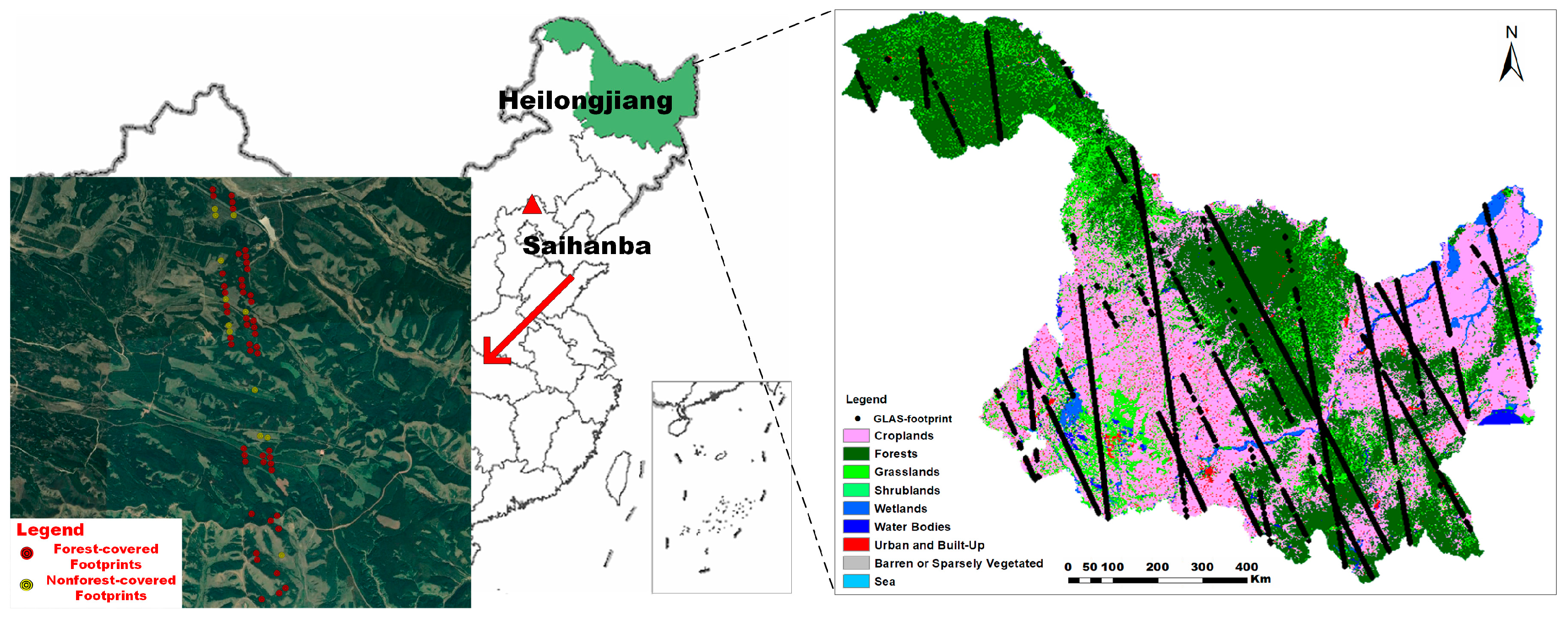
2.1. Study Area
2.2. GLAS Data
2.3. Ancillary Data
2.4. MODIS CI Products
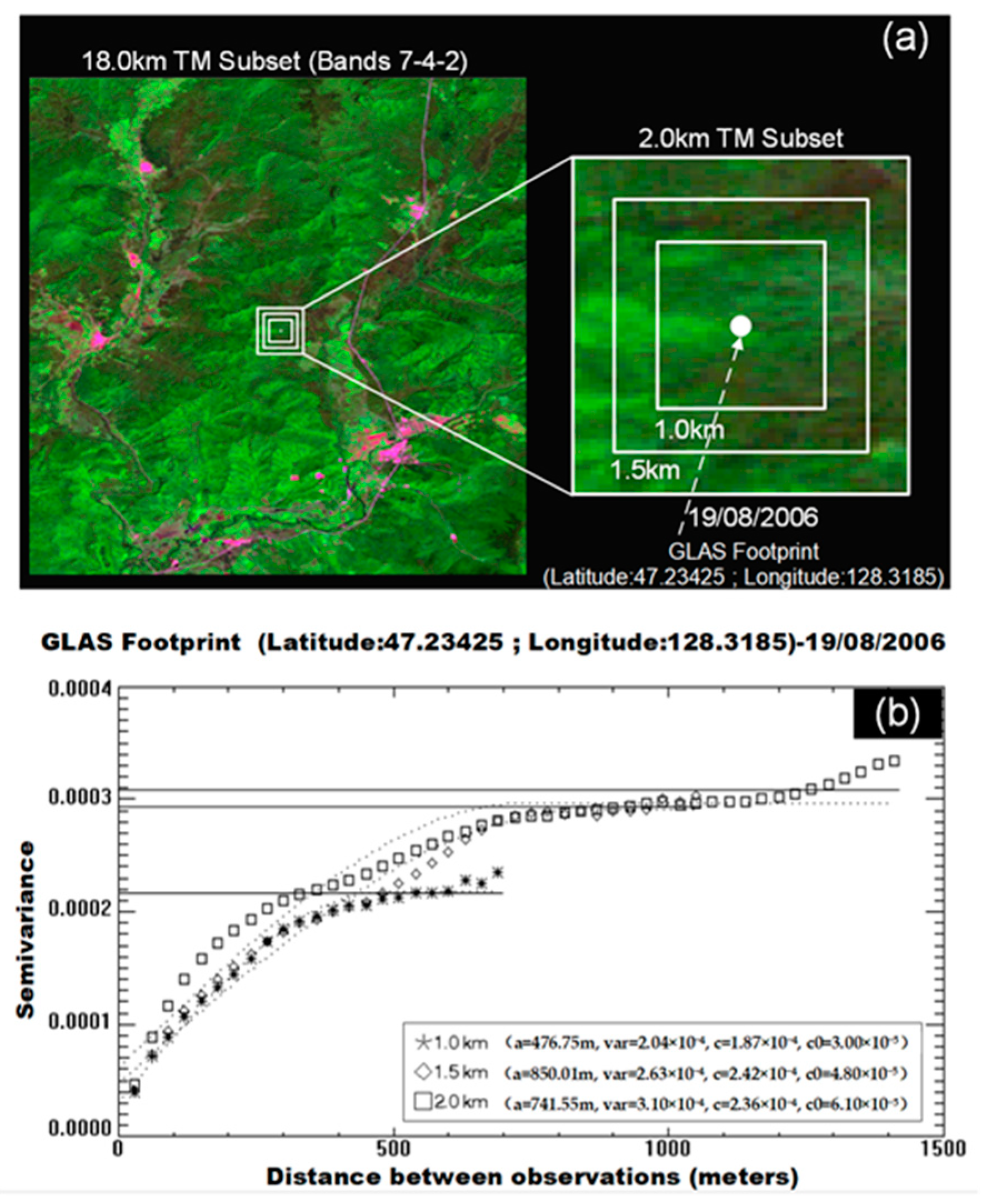
2.5. Data Used for Scale Effect Analysis
2.6. Ground-Based Data
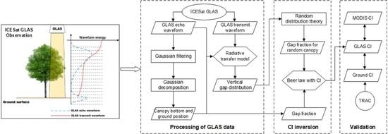
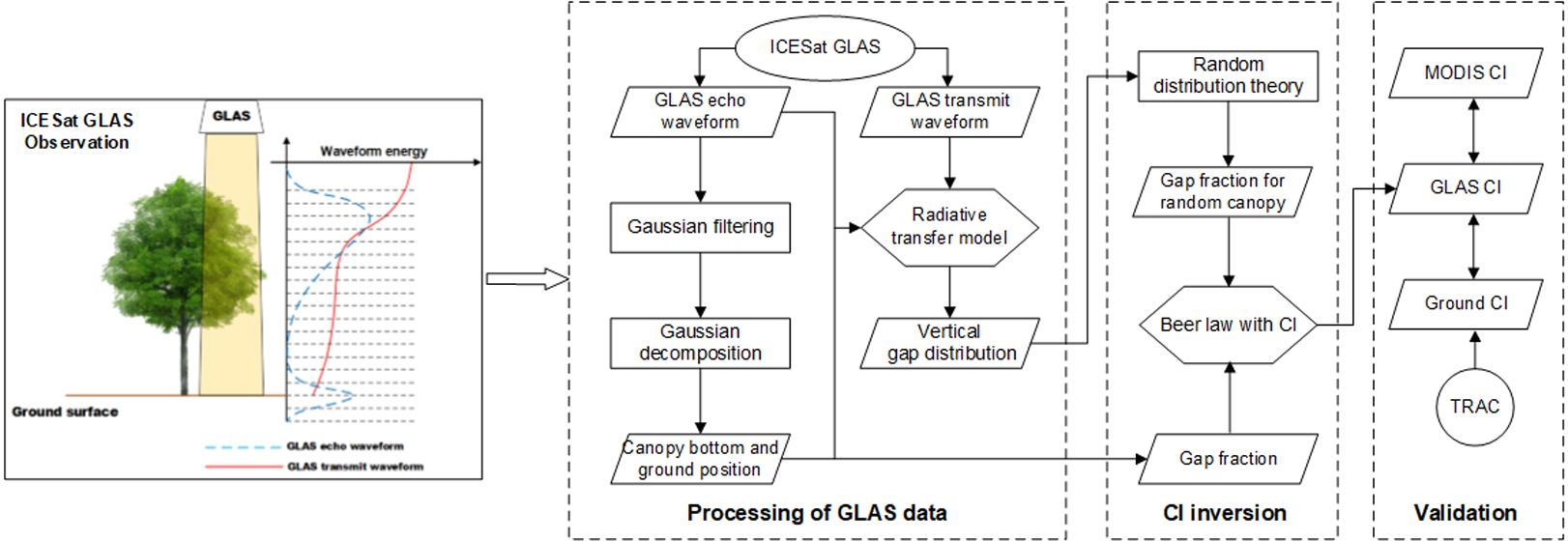
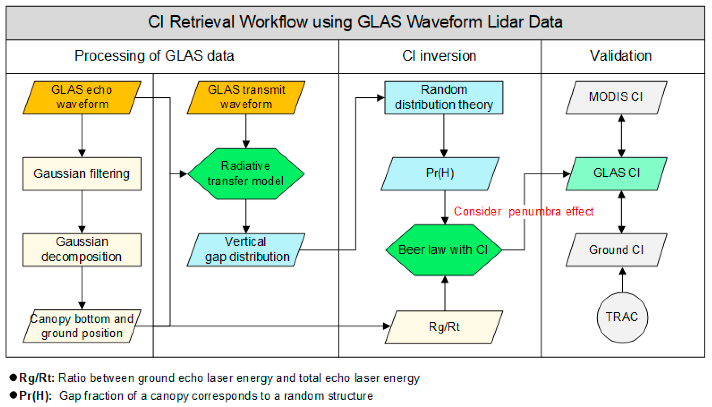
3. Methods
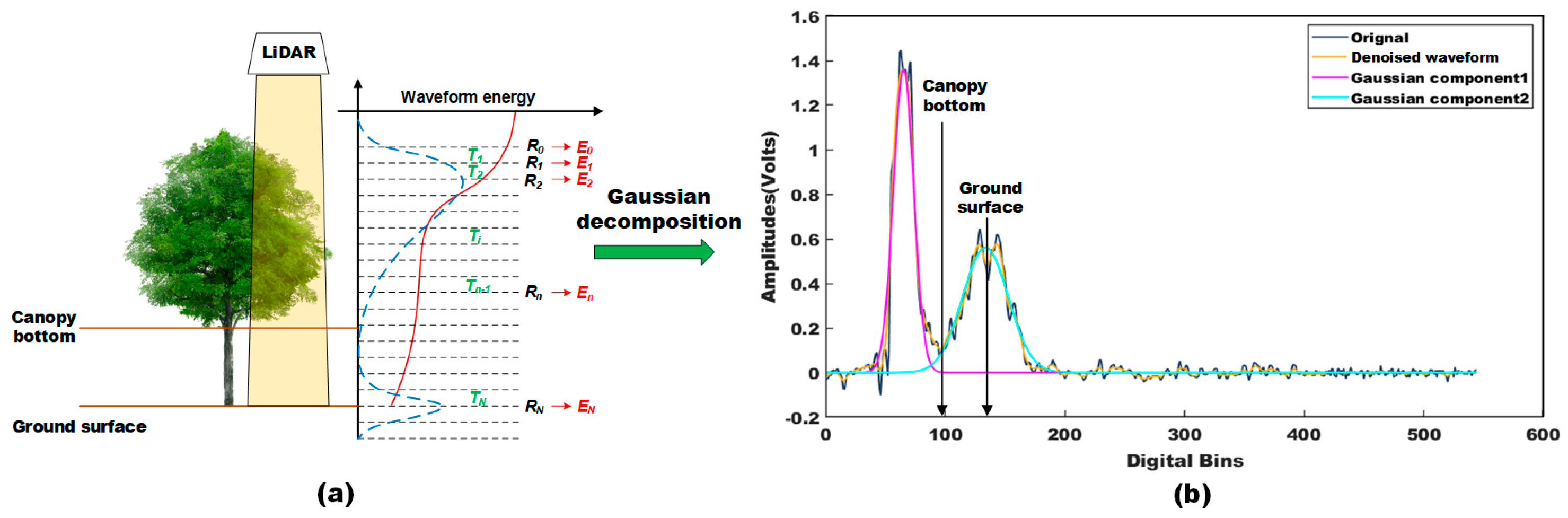
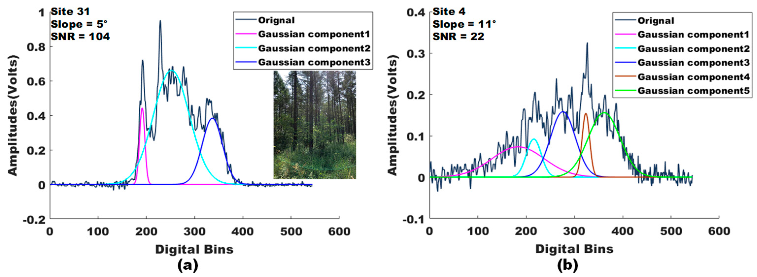
3.1. Processing of GLAS Data
3.1.1. Extraction of Canopy Bottom and Ground Position from GLAS Received Waveform
3.1.2. Calculation of Forest Vertical Gap Distribution Using GLAS data
3.2. CI Inversion
3.3. Validation
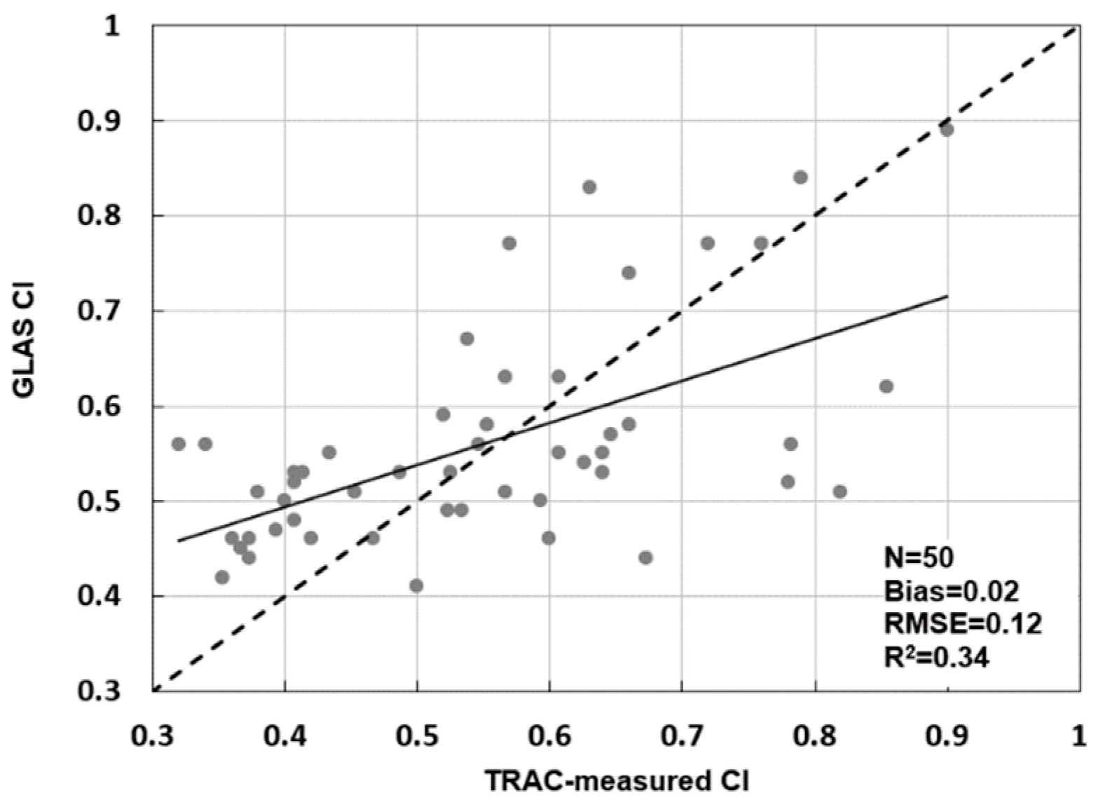
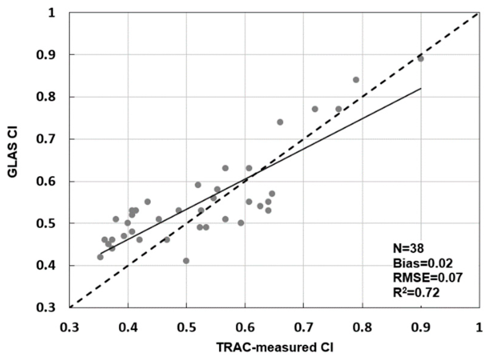
3.3.1. Comparison of GLAS CI and TRAC-Measured CI
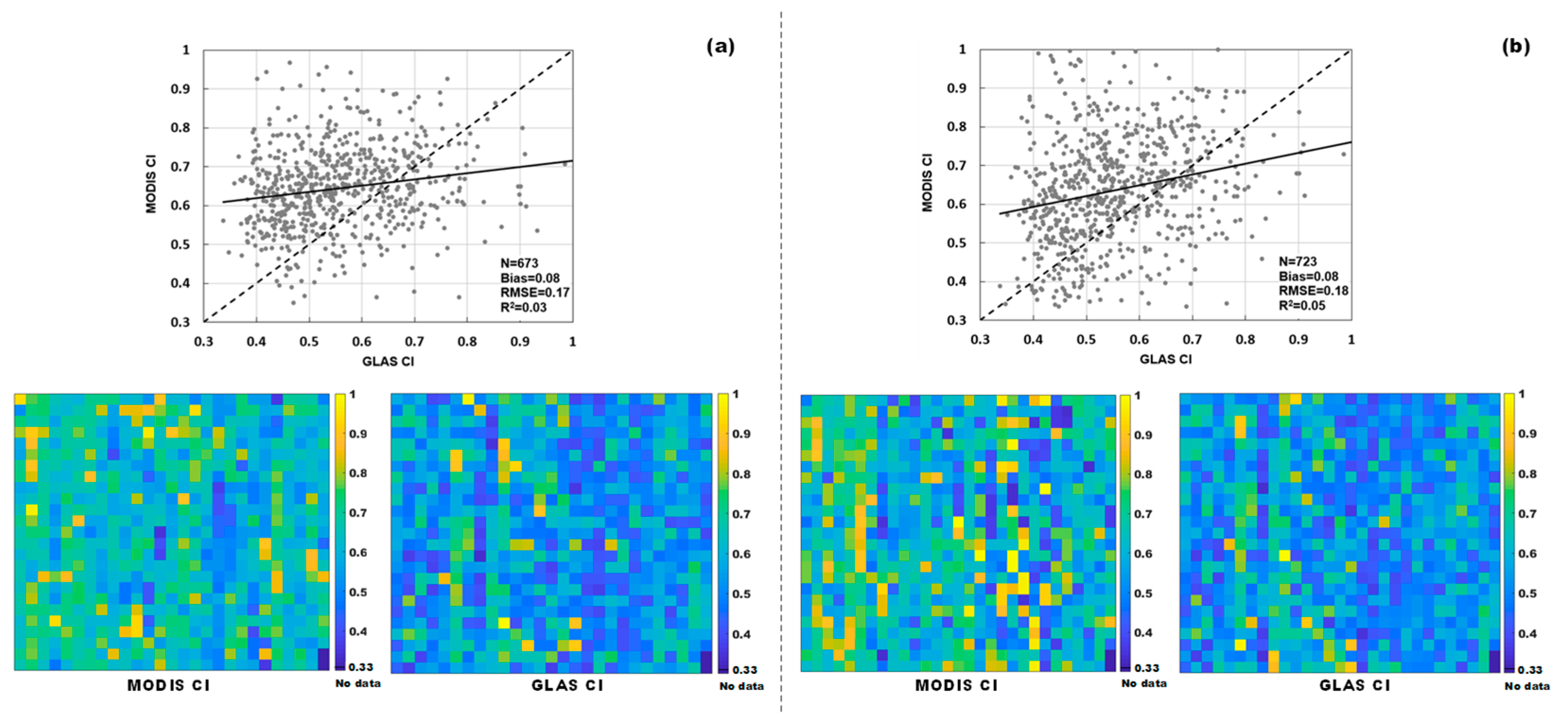
3.3.2. Comparison of GLAS CI and MODIS CI
4. Results and Analysis
4.1. GLAS CI vs. TRAC-Measured CI
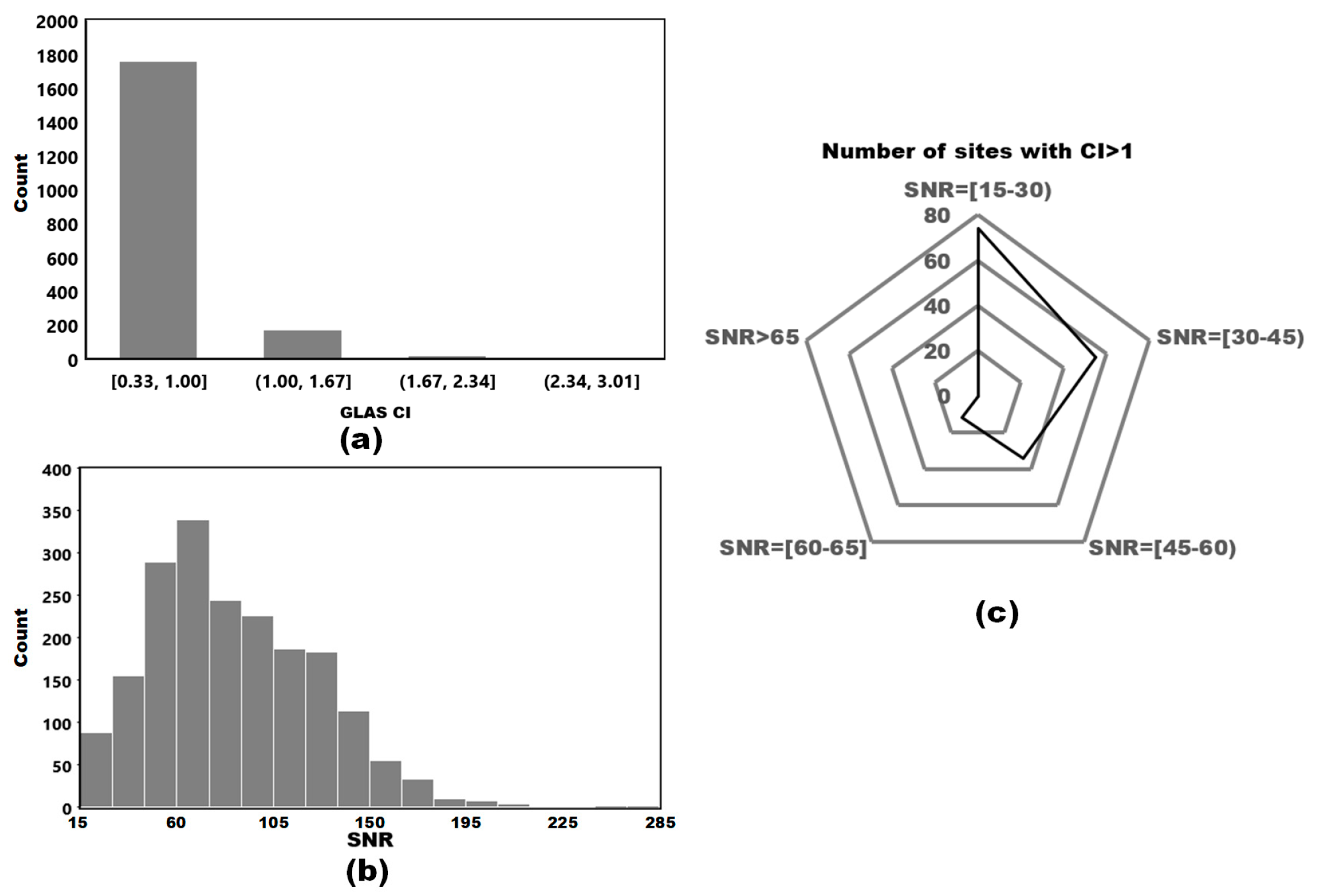
4.2. CI retrieval in Heilongjiang Province
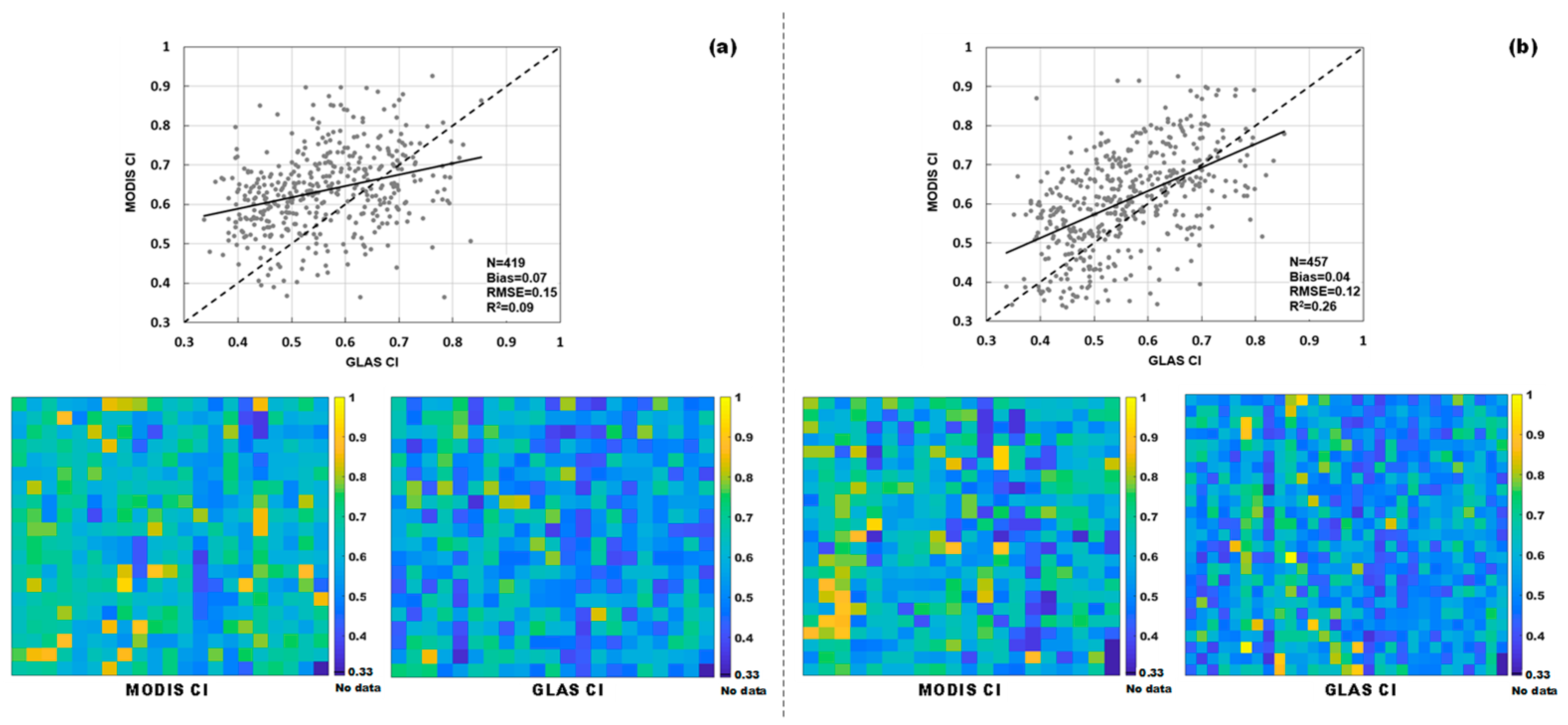
4.2.1. GLAS CI vs. MODIS CI
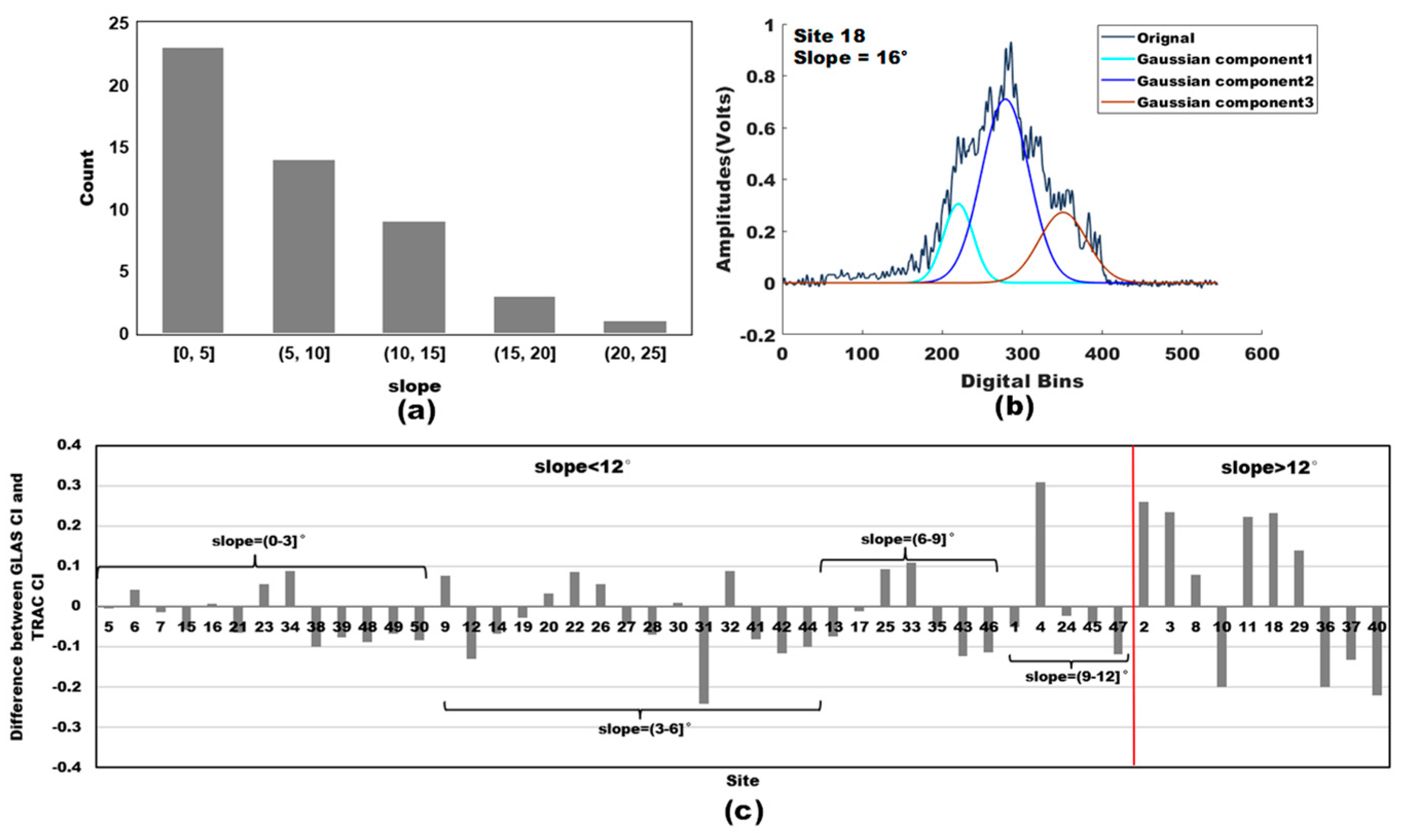
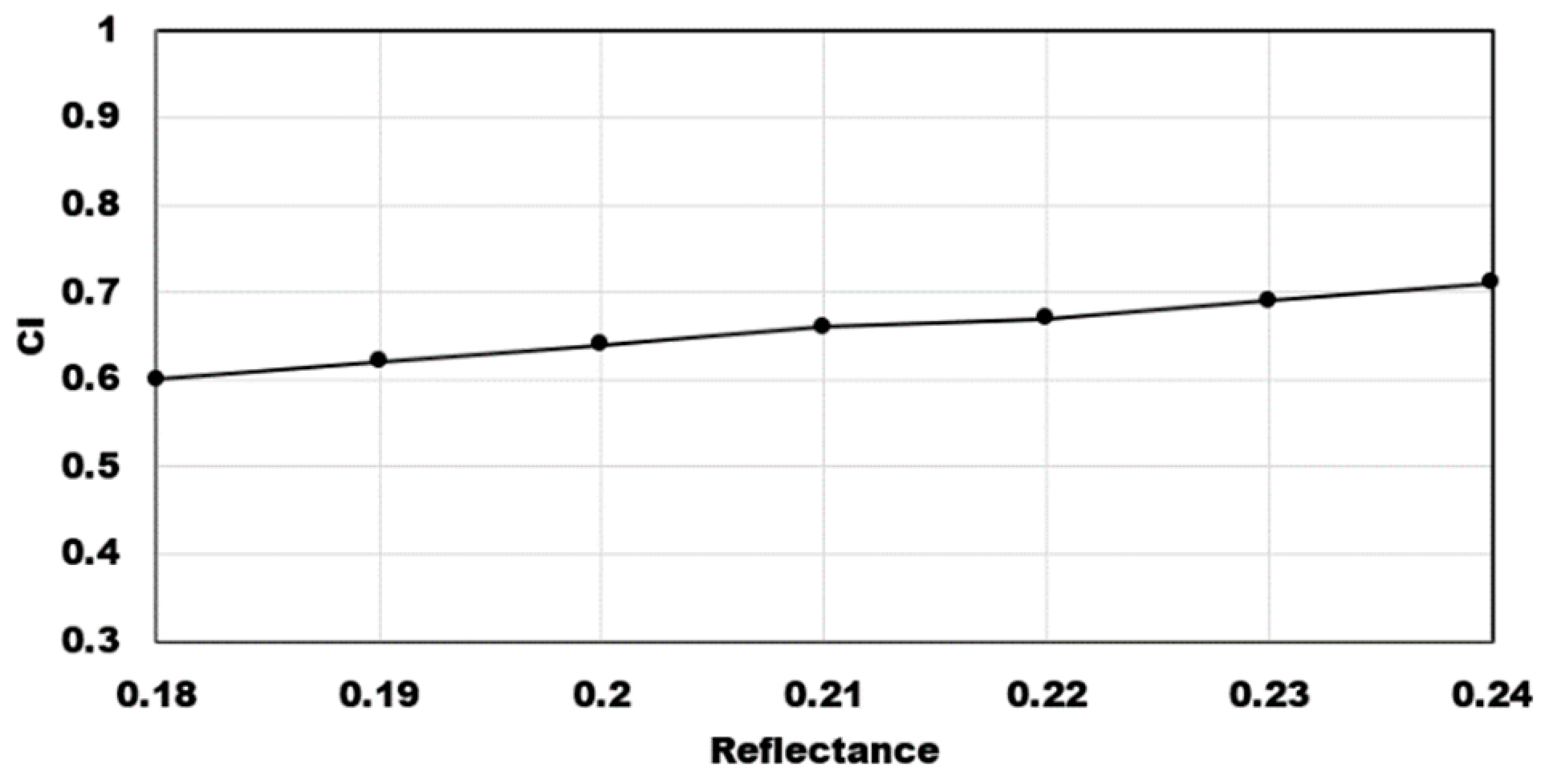
4.3. Model Uncertainty Analysis
5. Discussion
6. Conclusions
Author Contributions
Funding
Informed Consent Statement
Data Availability Statement
Conflicts of Interest
Appendix A
Appendix B

| GLAS ID | Latitude | Longitude | Vegetation Types | γ | Ωe(θ) | Field CI | ||
|---|---|---|---|---|---|---|---|---|
| Site | i_rec_ndx | i_shot_cout | ||||||
| 1 | 219109634 | 5 | 42.357381 | 117.35471 | birch | 1 | 0.77 | 0.77 |
| 2 | 219109634 | 11 | 42.366674 | 117.35291 | birch | 1 | 0.52 | 0.52 |
| 3 | 219109634 | 12 | 42.368221 | 117.35260 | birch | 1 | 0.62 | 0.62 |
| 4 | 219109634 | 18 | 42.377491 | 117.35078 | birch | 1 | 0.51 | 0.51 |
| 5 | 219109634 | 26 | 42.389872 | 117.34837 | larch | 1.5 | 0.8 | 0.53 |
| 6 | 219109634 | 27 | 42.391422 | 117.34806 | larch | 1.5 | 0.74 | 0.49 |
| 7 | 219109634 | 28 | 42.392973 | 117.34776 | larch | 1.5 | 0.84 | 0.56 |
| 8 | 219109639 | 4 | 42.419341 | 117.34263 | larch | 1.5 | 0.87 | 0.58 |
| 9 | 219109639 | 5 | 42.417794 | 117.34293 | larch | 1.5 | 0.86 | 0.57 |
| 10 | 219109639 | 9 | 42.427073 | 117.34111 | birch | 1 | 0.77 | 0.77 |
| 11 | 219109639 | 10 | 42.425525 | 117.34141 | birch | 1 | 0.56 | 0.56 |
| 12 | 219109639 | 12 | 42.430165 | 117.3405 | larch | 1.5 | 0.77 | 0.51 |
| 13 | 219109639 | 13 | 42.431711 | 117.3402 | larch | 1.5 | 0.72 | 0.48 |
| 14 | 219109639 | 15 | 42.434803 | 117.33959 | larch | 1.5 | 0.66 | 0.44 |
| 15 | 219109639 | 27 | 42.453392 | 117.33596 | larch | 1.5 | 0.77 | 0.51 |
| 16 | 219109639 | 28 | 42.454943 | 117.33566 | larch | 1.5 | 0.69 | 0.46 |
| 17 | 377874826 | 1 | 42.36017 | 117.36226 | birch | 1 | 0.77 | 0.77 |
| 18 | 377874826 | 10 | 42.37410 | 117.35957 | larch | 1.5 | 0.66 | 0.44 |
| 19 | 377874826 | 12 | 42.37718 | 117.35896 | larch | 1.5 | 0.87 | 0.58 |
| 20 | 377874826 | 19 | 42.387999 | 117.35687 | larch | 1.5 | 0.74 | 0.49 |
| 21 | 377874826 | 20 | 42.389544 | 117.35657 | larch | 1.5 | 0.95 | 0.63 |
| 22 | 377874826 | 21 | 42.391089 | 117.35627 | larch | 1.5 | 0.81 | 0.54 |
| 23 | 377874826 | 22 | 42.392634 | 117.35597 | larch | 1.5 | 0.77 | 0.51 |
| 24 | 377874826 | 37 | 42.415832 | 117.35146 | larch | 1.5 | 0.95 | 0.63 |
| 25 | 377874826 | 38 | 42.41738 | 117.35115 | larch | 1.5 | 0.75 | 0.50 |
| 26 | 377874826 | 40 | 42.420475 | 117.35055 | larch | 1.5 | 0.83 | 0.55 |
| 27 | 377874831 | 1 | 42.422022 | 117.35024 | larch | 1.5 | 0.8 | 0.53 |
| 28 | 377874831 | 2 | 42.423569 | 117.34994 | larch | 1.5 | 0.89 | 0.59 |
| 29 | 377874831 | 5 | 42.428203 | 117.34904 | larch | 1.5 | 0.69 | 0.46 |
| 30 | 377874831 | 6 | 42.42975 | 117.34874 | birch | 1 | 0.89 | 0.89 |
| 31 | 377874831 | 10 | 42.435944 | 117.347562 | larch | 1.5 | 0.84 | 0.56 |
| 32 | 377874831 | 11 | 42.437491 | 117.34726 | larch | 1.5 | 0.62 | 0.41 |
| 33 | 377874831 | 12 | 42.439036 | 117.34696 | larch | 1.5 | 0.8 | 0.53 |
| 34 | 377874831 | 13 | 42.44058 | 117.34666 | larch | 1.5 | 0.82 | 0.55 |
| 35 | 537071457 | 1 | 42.358912 | 117.36027 | birch | 1 | 0.84 | 0.84 |
| 36 | 537071457 | 4 | 42.363587 | 117.35937 | birch | 1 | 0.83 | 0.83 |
| 37 | 537071457 | 12 | 42.375961 | 117.356948 | mixed forest | 1.43 | 0.96 | 0.67 |
| 38 | 537071457 | 21 | 42.389854 | 117.35421 | larch | 1.5 | 0.75 | 0.50 |
| 39 | 537071457 | 22 | 42.391403 | 117.35391 | larch | 1.5 | 0.7 | 0.47 |
| 40 | 537071457 | 38 | 42.416399 | 117.3491 | larch | 1.5 | 0.84 | 0.56 |
| 41 | 537071457 | 39 | 42.41796 | 117.3488 | birch | 1 | 0.74 | 0.74 |
| 42 | 537071462 | 2 | 42.422629 | 117.34788 | mixed forest | 1.43 | 0.79 | 0.55 |
| 43 | 537071462 | 3 | 42.424179 | 117.34758 | larch | 1.5 | 0.8 | 0.53 |
| 44 | 537071462 | 7 | 42.430353 | 117.34636 | larch | 1.5 | 0.69 | 0.46 |
| 45 | 537071462 | 8 | 42.431895 | 117.34606 | larch | 1.5 | 0.69 | 0.46 |
| 46 | 537071462 | 9 | 42.433434 | 117.34576 | larch | 1.5 | 0.78 | 0.52 |
| 47 | 537071462 | 13 | 42.439595 | 117.34455 | larch | 1.5 | 0.8 | 0.53 |
| 48 | 537071462 | 20 | 42.450446 | 117.34242 | larch | 1.5 | 0.69 | 0.46 |
| 49 | 537071462 | 21 | 42.452004 | 117.34212 | larch | 1.5 | 0.63 | 0.42 |
| 50 | 537071462 | 22 | 42.453564 | 117.34182 | larch | 1.5 | 0.68 | 0.45 |
References
- Chen, J.M.; Black, T.A. Foliage Area and Architecture of Plant Canopies from Sunfleck Size Disributions. Agric. Forest Meteorol. 1992, 60, 249–266. [Google Scholar] [CrossRef]
- Nilson, T. Theoretical Analysis of Frequency of Gaps in Plant Stands. Agric. Meteorol. 1971, 8, 25. [Google Scholar] [CrossRef]
- Xiao, Z.; Liang, S.; Wang, J.; Chen, P.; Yin, X.; Zhang, L.; Song, J. Use of General Regression Neural Networks for Generating the Glass Leaf Area Index Product from Time-Series Modis Surface Reflectance. IEEE Trans. Geosci. Remote 2014, 52, 209–223. [Google Scholar] [CrossRef]
- Deng, F.; Chen, J.M.; Plummer, S.; Chen, M.; Pisek, J. Algorithm for Global Leaf Area Index Retrieval Using Satellite Imagery. IEEE Trans. Geosci. Remote 2006, 44, 2219–2229. [Google Scholar] [CrossRef]
- Liu, Y.; Liu, R.; Chen, J.M. Retrospective Retrieval of Long-Term Consistent Global Leaf Area Index (1981–2011) From Combined Avhrr and Modis Data. J. Geophys. Res. Biogeosci. 2012, 117, G04003. [Google Scholar] [CrossRef]
- Chen, J.M.; Liu, J.; Cihlar, J.; Goulden, M.L. Daily Canopy Photosynthesis Model through Temporal and Spatial Scaling for Remote Sensing Applications. Ecol. Model. 1999, 124, 99–119. [Google Scholar] [CrossRef]
- He, L.; Chen, J.M.; Gonsamo, A.; Luo, X.; Wang, R.; Liu, Y.; Liu, R. Changes in the Shadow: The Shifting Role of Shaded Leaves in Global Carbon and Water Cycles Under Climate Change. Geophys. Res. Lett. 2018, 45, 5052–5061. [Google Scholar] [CrossRef]
- Ryu, Y.; Baldocchi, D.D.; Kobayashi, H.; van Ingen, C.; Li, J.; Black, T.A.; Beringer, J.; van Gorsel, E.; Knohl, A.; Law, B.E.; et al. Integration of Modis Land and Atmosphere Products with a Coupled-Process Model to Estimate Gross Primary Productivity and Evapotranspiration From 1 Km to Global Scales. Glob. Biogeochem. Cycles 2011, 25, GB4017. [Google Scholar] [CrossRef]
- Chen, J.M.; Mo, G.; Pisek, J.; Liu, J.; Deng, F.; Ishizawa, M.; Chan, D. Effects of Foliage Clumping on the Estimation of Global Terrestrial Gross Primary Productivity. Glob. Biogeochem. Cycles 2012, 26, 1–18. [Google Scholar]
- Chen, B.; Liu, J.; Chen, J.M.; Croft, H.; Gonsamo, A.; He, L.; Luo, X. Assessment of Foliage Clumping Effects on Evapotranspiration Estimates in Forested Ecosystems. Agric. Forest Meteorol. 2016, 216, 82–92. [Google Scholar] [CrossRef]
- Chen, J.M.; Menges, C.H.; Leblanc, S.G. Global Mapping of Foliage Clumping Index Using Multi-Angular Satellite Data. Remote Sens. Environ. 2005, 97, 447–457. [Google Scholar] [CrossRef]
- Chen, J.M.; Leblanc, S.G. A Four-Scale Bidirectional Reflectance Model Based on Canopy Architecture. IEEE Trans. Geosci. Remote 1997, 35, 1316–1337. [Google Scholar] [CrossRef]
- Jiao, Z.; Schaaf, C.B.; Dong, Y.; Román, M.; Hill, M.J.; Chen, J.M.; Wang, Z.; Zhang, H.; Saenz, E.; Poudyal, R.; et al. A Method for Improving Hotspot Directional Signatures in Brdf Models Used for Modis. Remote Sens. Environ. 2016, 186, 135–151. [Google Scholar] [CrossRef]
- Pisek, J.; Chen, J.M.; Lacaze, R.; Sonnentag, O.; Alikas, K. Expanding Global Mapping of the Foliage Clumping Index with Multi-Angular Polder Three Measurements: Evaluation and Topographic Compensation. ISPRS J. Photogramm. 2010, 65, 341–346. [Google Scholar] [CrossRef]
- Wei, S.; Fang, H.; Schaaf, C.B.; He, L.; Chen, J.M. Global 500 M Clumping Index Product Derived from Modis Brdf Data (2001–2017). Remote Sens. Environ. 2019, 232, 111296. [Google Scholar] [CrossRef]
- He, L.; Chen, J.M.; Pisek, J.; Schaaf, C.B.; Strahler, A.H. Global Clumping Index Map Derived from the Modis Brdf Product. Remote Sens. Environ. 2012, 119, 118–130. [Google Scholar] [CrossRef]
- Jiao, Z.; Dong, Y.; Schaaf, C.B.; Chen, J.M.; Román, M.; Wang, Z.; Zhang, H.; Ding, A.; Erb, A.; Hill, M.J.; et al. An Algorithm for the Retrieval of the Clumping Index (Ci) From the Modis Brdf Product Using an Adjusted Version of the Kernel-Driven Brdf Model. Remote Sens. Environ. 2018, 209, 594–611. [Google Scholar] [CrossRef]
- Pisek, J.; Ryu, Y.; Sprintsin, M.; He, L.; Oliphant, A.J.; Korhonen, L.; Kuusk, J.; Kuusk, A.; Bergstrom, R.; Verrelst, J.; et al. Retrieving Vegetation Clumping Index from Multi-Angle Imaging Spectroradiometer (Misr) Data at 275M Resolution. Remote Sens. Environ. 2013, 138, 126–133. [Google Scholar] [CrossRef]
- Wei, S.; Fang, H. Estimation of Canopy Clumping Index from Misr and Modis Sensors Using the Normalized Difference Hotspot and Darkspot (Ndhd) Method: The Influence of Brdf Models and Solar Zenith Angle. Remote Sens. Environ. 2016, 187, 476–491. [Google Scholar] [CrossRef]
- Maignan, F.; Breon, F.M.; Lacaze, R. Bidirectional Reflectance of Earth Targets: Evaluation of Analytical Models Using a Large Set of Spaceborne Measurements with Emphasis on the Hot Spot. Remote Sens. Environ. 2004, 90, 210–220. [Google Scholar] [CrossRef]
- Brovelli, M.A.; Crespi, M.; Fratarcangeli, F.; Giannone, F.; Realini, E. Accuracy Assessment of High Resolution Satellite Imagery Orientation by Leave-One-Out Method (Article). ISPRS J. Photogramm. 2008, 63, 427–440. [Google Scholar] [CrossRef]
- Goetz, S.J. Synergistic Use of Spaceborne Lidar and Optical Imagery for Assessing Forest Disturbance: An Alaska Case Study. J. Geophys. Res. Biogeosci. 2010, 115, G00E07. [Google Scholar] [CrossRef]
- Mitchell, J.J.; Shrestha, R.; Spaete, L.P.; Glenn, N.F. Combining Airborne Hyperspectral and Lidar Data Across Local Sites for Upscaling Shrubland Structural Information: Lessons for Hyspiri. Remote Sens. Environ. 2015, 167, 98–110. [Google Scholar] [CrossRef]
- García, M.; Gajardo, J.; Riaño, D.; Zhao, K.; Martín, P.; Ustin, S. Canopy Clumping Appraisal Using Terrestrial and Airborne Laser Scanning. Remote Sens. Environ. 2015, 161, 78–88. [Google Scholar] [CrossRef]
- Li, Y.; Guo, Q.; Su, Y.; Tao, S.; Zhao, K.; Xu, G. Retrieving the Gap Fraction, Element Clumping Index, and Leaf Area Index of Individual Trees Using Single-Scan Data from a Terrestrial Laser Scanner. ISPRS J. Photogramm. Remote Sens. 2017, 130, 308–316. [Google Scholar] [CrossRef]
- Ma, L.; Zheng, G.; Wang, X.; Li, S.; Lin, Y.; Ju, W. Retrieving Forest Canopy Clumping Index Using Terrestrial Laser Scanning Data. Remote Sens. Environ. 2018, 210, 452–472. [Google Scholar] [CrossRef]
- Zhao, K.; Ryu, Y.; Hu, T.; Garcia, M.; Li, Y.; Liu, Z.; Londo, A.; Wang, C.; Chisholm, R. How to Better Estimate Leaf Area Index and Leaf Angle Distribution from Digital Hemispherical Photography? Switching to a Binary Nonlinear Regression Paradigm. Methods Ecol. Evol. 2019, 10, 1864–1874. [Google Scholar] [CrossRef]
- Thomas, V.T.V.E.; Noland, T.; Treitz, P.; McCaughey, J.H. Leaf Area and Clumping Indices for a Boreal Mixed-Wood Forest: Lidar, Hyperspectral, and Landsat Models. Int. J. Remote Sens. 2011, 32, 8271–8297. [Google Scholar] [CrossRef]
- Zhao, F.; Strahler, A.H.; Schaaf, C.L.; Yao, T.; Yang, X.; Wang, Z.; Schull, M.A.; Román, M.O.; Woodcock, C.E.; Olofsson, P.; et al. Measuring Gap Fraction, Element Clumping Index and Lai in Sierra Forest Stands Using a Full-Waveform Ground-Based Lidar. Remote Sens. Environ. 2012, 125, 73–79. [Google Scholar] [CrossRef]
- Kuusk, A.; Pisek, J.; Lang, M.; Märdla, S. Estimation of Gap Fraction and Foliage Clumping in Forest Canopies. Remote Sens. Basel 2018, 10, 1153. [Google Scholar] [CrossRef]
- Cui, L.; Jiao, Z.; Zhao, K.; Sun, M.; Dong, Y.; Yin, S.; Li, Y.; Chang, Y.; Guo, J.; Xie, R.; et al. Retrieval of Vertical Foliage Profile and Leaf Area Index Using Transmitted Energy Information Derived from Icesat Glas Data. Remote Sens. Basel 2020, 12, 2457. [Google Scholar] [CrossRef]
- Dubayah, R.; Blair, J.B.; Goetz, S.; Fatoyinbo, L.; Hansen, M.; Healey, S.; Hofton, M.; Hurtt, G.; Kellner, J.; Luthcke, S.; et al. The Global Ecosystem Dy-namics Investigation: High-Resolution Laser Ranging of the Earth’S Forests and Topography. Sci. Remote Sens. 2020, 1, 100002. [Google Scholar] [CrossRef]
- Heilongjiang Forestry and Grassland Bureau. Available online: http://hljforest.com/ (accessed on 18 December 2020).
- National Geomatics Center of China (NGCC). 30-Meter Global Land Cover Dataset (GlobeLand30)-Product Description Data. 2014. Available online: http://www.globallandcover.com/GLC30Download/index.aspx (accessed on 20 January 2020).
- Jun, C.; Ban, Y.; Li, S. Open Access to Earth Land-Cover Map. Nature 2014, 514, 434. [Google Scholar] [CrossRef] [PubMed]
- Pang, Y.; Li, Z.; Lefsky, M.; Guoqing, S.; Yu, X. Model Based Terrain Effect Analyses on ICEsat GLAS Waveforms. In Proceedings of the 2006 IEEE International Symposium on Geoscience and Remote Sensing, Denver, CO, USA, 31 July–4 August 2006; p. 3232. [Google Scholar]
- Farr, T.G.; Rosen, P.A.; Caro, E.; Crippen, R.; Duren, R.; Hensley, S.; Kobrick, M.; Paller, M.; Rodriguez, E.; Roth, L.; et al. The Shuttle Radar Topography Mission. Rev. Geophys. 2007, 45, 2005RG000183. [Google Scholar] [CrossRef]
- Hansen, M.C.; DeFries, R.S.; Townshend, J.R.G.; Carroll, M.; Dimiceli, C.; Sohlberg, R.A. Global Percent Tree Cover at a Spatial Resolution of 500 Meters: First Results of the Modis Vegetation Continuous Fields Algorithm. Earth Interact. 2003, 7, 1–15. [Google Scholar] [CrossRef]
- Wang, Z.; Schaaf, C.B.; Strahler, A.H.; Chopping, M.J.; Roman, M.O.; Shuai, Y.; Woodcock, C.E.; Hollinger, D.Y.; Fitzjarrald, D.R. Evaluation of Modis Albedo Product (Mcd43a) Over Grassland, Agriculture and Forest Surface Types During Dormant and Snow-Covered Periods. Remote Sens. Environ. 2014, 140, 60–77. [Google Scholar] [CrossRef]
- Roman, M.O.; Schaaf, C.B.; Woodcock, C.E.; Strahler, A.H.; Yang, X.; Braswell, R.H.; Curtis, P.S.; Davis, K.J.; Dragoni, D.; Goulden, M.L.; et al. The Modis (Collection V005) Brdf/Albedo Product: Assessment of Spatial Representativeness over Forested Landscapes. Remote Sens. Environ. 2009, 113, 2476–2498. [Google Scholar] [CrossRef]
- Pisek, J.; Chen, J.M.; Nilson, T. Estimation of Vegetation Clumping Index Using Modis Brdf Data. Int. J. Remote Sens. 2011, 32, 2645–2657. [Google Scholar] [CrossRef]
- Chen, J.M.; Cihlar, J. Plant Canopy Gap-Size Analysis Theory for Improving Optical Measurements of Leaf-Area Index. Appl. Opt. 1995, 34, 6211–6222. [Google Scholar] [CrossRef]
- Duong, V.H.; Lindenbergh, R.; Pfeifer, N.; Vosselman, G. Single and Two Epoch Analysis of Icesat Full Waveform Data Over Forested Areas. Int. J. Remote Sens. 2008, 29, 1453–1473. [Google Scholar] [CrossRef]
- Hofton, M.A.; Minster, J.B.; Blair, J.B. Decomposition of Laser Altimeter Waveforms. IEEE Trans. Geosci. Remote 2000, 38, 1989–1996. [Google Scholar] [CrossRef]
- Yang, X.; Wang, C.; Pan, F.; Nie, S.; Xi, X.; Luo, S. Retrieving Leaf Area Index in Discontinuous Forest Using Icesat/Glas Full-Waveform Data Based on Gap Fraction Model. ISPRS J. Photogramm. 2019, 148, 54–62. [Google Scholar] [CrossRef]
- Luo, S.; Wang, C.; Li, G.; Xi, X. Retrieving Leaf Area Index Using Icesat/Glas Full-Waveform Data. Remote Sens. Lett. 2013, 4, 745–753. [Google Scholar] [CrossRef]
- Chen, J.M. Optically-Based Methods for Measuring Seasonal Variation of Leaf Area Index in Boreal Conifer Stands. Agric. Forest Meteorol. 1996, 80, 135–163. [Google Scholar] [CrossRef]
- Wang, Z.; Schaaf, C.B.; Sun, Q.; Kim, J.; Erb, A.M.; Gao, F.; Roman, M.O.; Yang, Y.; Petroy, S.; Taylor, J.R.; et al. Monitoring Land Surface Albedo and Vegetation Dynamics Using High Spatial and Temporal Resolution Synthetic Time Series from Landsat and the Modis Brdf/Nbar/Albedo Product. Int. J. Appl. Earth Obs. 2017, 59, 104–117. [Google Scholar] [CrossRef] [PubMed]
- Huang, H.; Liu, C.; Wang, X.; Biging, G.S.; Chen, Y.; Yang, J.; Gong, P. Mapping Vegetation Heights in China Using Slope Correction Icesat Data, Srtm, Modis-Derived and Climate Data. ISPRS J. Photogramm. 2017, 129, 189–199. [Google Scholar] [CrossRef]
- Tang, H.; Dubayah, R.; Brolly, M.; Ganguly, S.; Zhang, G. Large-Scale Retrieval of Leaf Area Index and Vertical Foliage Profile from the Spaceborne Waveform Lidar (Glas/Icesat). Remote Sens. Environ. 2014, 154, 8–18. [Google Scholar] [CrossRef]
- Wang, X.; Huang, H.; Gong, P.; Liu, C.; Li, C.; Li, W. Forest Canopy Height Extraction in Rugged Areas with Icesat/Glas Data. IEEE Trans. Geosci. Remote 2014, 52, 4650–4657. [Google Scholar] [CrossRef]
- Harding, D.J. Icesat Waveform Measurements of within-Footprint Topographic Relief and Vegetation Vertical Structure. Geophys. Res. Lett. 2005, 32, L21S10. [Google Scholar] [CrossRef]
- Popescu, S.C.; Zhao, K.; Neuenschwander, A.; Lin, C. Satellite Lidar Vs. Small Footprint Airborne Lidar: Comparing the Accuracy of Aboveground Biomass Estimates and Forest Structure Metrics at Footprint Level. Remote Sens. Environ. 2011, 115, 2786–2797. [Google Scholar] [CrossRef]
- Nie, S.; Wang, C.; Li, G.; Pan, F.; Xi, X.; Luo, S. Signal-to-Noise Ratio-Based Quality Assessment Method for Icesat/Glas Waveform Data. Opt. Eng. 2014, 53, 103104. [Google Scholar] [CrossRef]
- Wang, M.; Sun, R.; Xiao, Z. Estimation of Forest Canopy Height and Aboveground Biomass from Spaceborne Lidar and Landsat Imageries in Maryland. Remote Sens. Basel 2018, 10, 344. [Google Scholar] [CrossRef]
- Wang, Z.; Schaaf, C.B.; Sun, Q.; Shuai, Y.; Roman, M.O. Capturing Rapid Land Surface Dynamics with Collection V006 Modis Brdf/Nbar/Albedo (Mcd43) Products. Remote Sens. Environ. 2018, 207, 50–64. [Google Scholar] [CrossRef]
- Lang, A.; Xiang, Y.Q. Estimation of Leaf-Area Index from Transmission of Direct Sunlight in Discontinuous Canopies. Agric. Forest Meteorol. 1986, 37, 229–243. [Google Scholar] [CrossRef]
- Leblanc, S.G.; Chen, J.M.; Fernandes, R.; Deering, D.W.; Conley, A. Methodology Comparison for Canopy Structure Parameters Extraction from Digital Hemispherical Photography in Boreal Forests. Agric. Forest Meteorol. 2005, 129, 187–207. [Google Scholar] [CrossRef]
- Yan, G.; Hu, R.; Luo, J.; Weiss, M.; Jiang, H.; Mu, X.; Xie, D.; Zhang, W. Review of Indirect Optical Measurements of Leaf Area Index: Recent Advances, Challenges, and Perspectives. Agric. Forest Meteorol. 2019, 265, 390–411. [Google Scholar] [CrossRef]
- Sun, X.; Abshire, J.B.; Borsa, A.A.; Fricker, H.A.; Yi, D.; DiMarzio, J.P.; Paolo, F.S.; Brunt, K.M.; Harding, D.J.; Neumann, G.A. Icesat/Glas Altimetry Measurements: Received Signal Dynamic Range and Saturation Correction. IEEE Trans. Geosci. Remote 2017, 55, 5440–5454. [Google Scholar] [CrossRef] [PubMed]


| Product | Attributes | Record Name in GLAS File |
|---|---|---|
| GLA01 & GLA05 & GLA14 | Record identification | i_rec_ndx |
| count | i_shot_count | |
| GLA01 | Transmitted pulse waveform | r_tx_wf |
| Received pulse waveform | r_rng_wf | |
| Starting address of the transmit pulse sample | i_TxWfStart | |
| Ending address of the range response | i_RespEndTime | |
| GLA05 | Gain value used for received pulse | i_gval_rcv |
| Gain value used for transmitted pulse | i_gval_tx | |
| GLA14 | Latitude | i_lat |
| Longitude | i_lon | |
| Standard deviation of background noise | i_sDevNsObl | |
| Maximum amplitude of signal | i_maxRecAmp | |
| Reflectivity | d_reflctUC | |
| Reflectivity correction factor for atmospheric effects | d_reflCor_atm |
| Parameter | Symbol | Unit | Values |
|---|---|---|---|
| GLAS sensor configuration parameter | S | dimensionless | Calculation process of S is shown in Appendix A. |
| GLAS sensor emitted total pulse energy intensity | volts | E0 is calculated by summing up the effective GLAS transmitted waveform recorded in the GLAS product (i.e., r_tx_wf). | |
| GLAS sensor received echo intensity at each recorded layer | Ri | volts | Ri is provided by the GLAS received waveform recorded in the GLAS product (i.e., r_rng_wf). |
Publisher’s Note: MDPI stays neutral with regard to jurisdictional claims in published maps and institutional affiliations. |
© 2021 by the authors. Licensee MDPI, Basel, Switzerland. This article is an open access article distributed under the terms and conditions of the Creative Commons Attribution (CC BY) license (http://creativecommons.org/licenses/by/4.0/).
Share and Cite
Cui, L.; Jiao, Z.; Zhao, K.; Sun, M.; Dong, Y.; Yin, S.; Zhang, X.; Guo, J.; Xie, R.; Zhu, Z.; et al. Retrieving Forest Canopy Elements Clumping Index Using ICESat GLAS Lidar Data. Remote Sens. 2021, 13, 948. https://doi.org/10.3390/rs13050948
Cui L, Jiao Z, Zhao K, Sun M, Dong Y, Yin S, Zhang X, Guo J, Xie R, Zhu Z, et al. Retrieving Forest Canopy Elements Clumping Index Using ICESat GLAS Lidar Data. Remote Sensing. 2021; 13(5):948. https://doi.org/10.3390/rs13050948
Chicago/Turabian StyleCui, Lei, Ziti Jiao, Kaiguang Zhao, Mei Sun, Yadong Dong, Siyang Yin, Xiaoning Zhang, Jing Guo, Rui Xie, Zidong Zhu, and et al. 2021. "Retrieving Forest Canopy Elements Clumping Index Using ICESat GLAS Lidar Data" Remote Sensing 13, no. 5: 948. https://doi.org/10.3390/rs13050948
APA StyleCui, L., Jiao, Z., Zhao, K., Sun, M., Dong, Y., Yin, S., Zhang, X., Guo, J., Xie, R., Zhu, Z., Li, S., & Tong, Y. (2021). Retrieving Forest Canopy Elements Clumping Index Using ICESat GLAS Lidar Data. Remote Sensing, 13(5), 948. https://doi.org/10.3390/rs13050948