Abstract
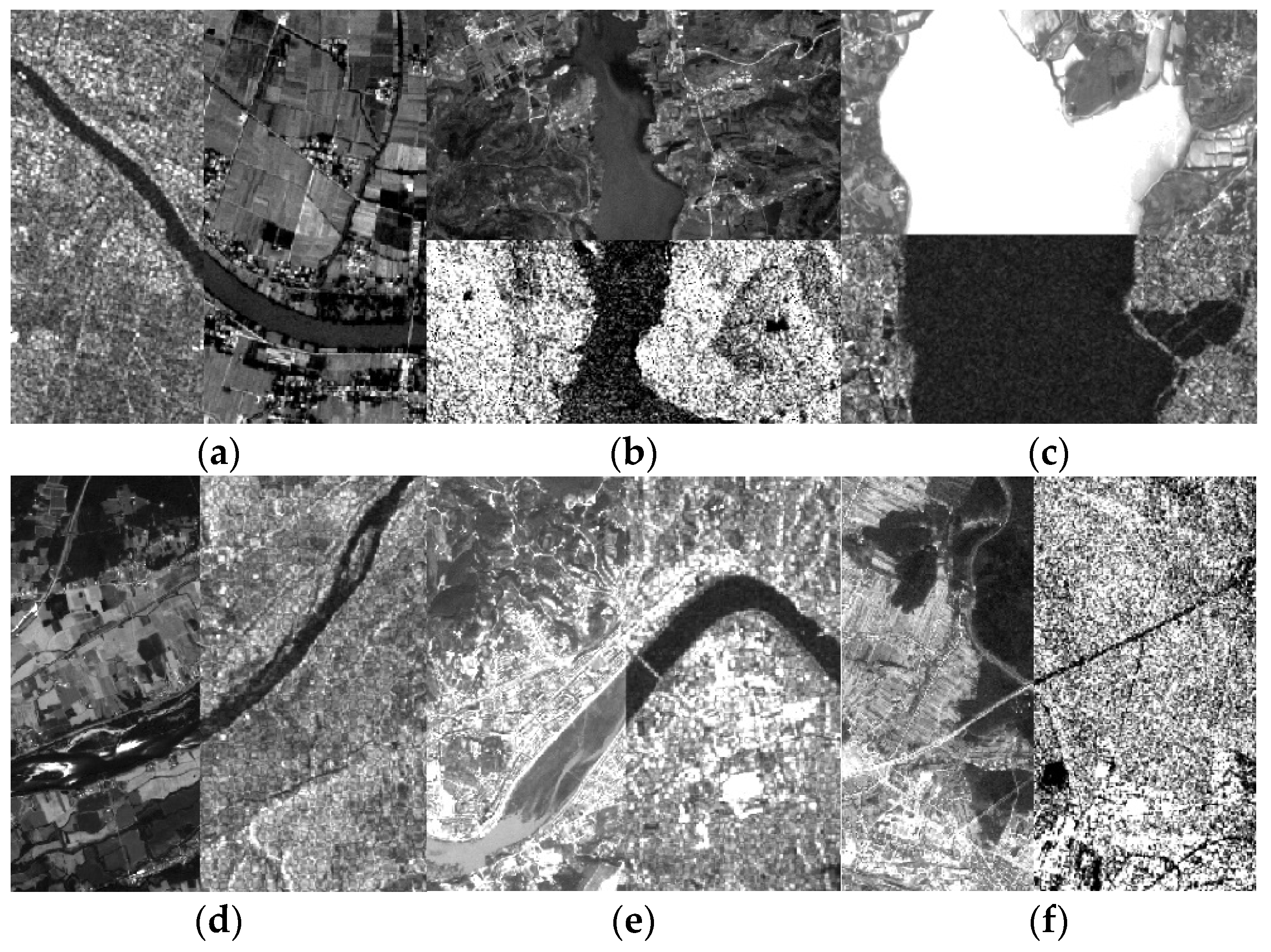
Co-registering the Sentinel-1 Synthetic Aperture Radar (SAR) and Sentinel-2 optical data of the European Space Agency (ESA) is of great importance for many remote sensing applications. However, we find that there are evident misregistration shifts between the Sentinel-1 SAR and Sentinel-2 optical images that are directly downloaded from the official website. To address that, this paper presents a fast and effective registration method for the two types of images. In the proposed method, a block-based scheme is first designed to extract evenly distributed interest points. Then, the correspondences are detected by using the similarity of structural features between the SAR and optical images, where the three-dimensional (3D) phase correlation (PC) is used as the similarity measure for accelerating image matching. Lastly, the obtained correspondences are employed to measure the misregistration shifts between the images. Moreover, to eliminate the misregistration, we use some representative geometric transformation models such as polynomial models, projective models, and rational function models for the co-registration of the two types of images, and we compare and analyze their registration accuracy under different numbers of control points and different terrains. Six pairs of the Sentinel-1 SAR L1 and Sentinel-2 optical L1C images covering three different terrains are tested in our experiments. Experimental results show that the proposed method can achieve precise correspondences between the images, and the third-order polynomial achieves the most satisfactory registration results. Its registration accuracy of the flat areas is less than 1.0 10 m pixel, that of the hilly areas is about 1.5 10 m pixels, and that of the mountainous areas is between 1.7 and 2.3 10 m pixels, which significantly improves the co-registration accuracy of the Sentinel-1 SAR and Sentinel-2 optical images.
1. Introduction
Sentinel-1 and 2 are special satellite series of European Copernicus program created by the European Space Agency (ESA). Equipped with new space sensors, Sentinel serial satellites carry out global observation with high revisit rate, and they use special wave bands to monitor the Earth surface. At present, Sentinel-1 Synthetic Aperture Radar (SAR) and Sentinel-2 Multiple Spectral Image (MSI) sensors have steadily provided products to the public. The public can download their original data (Level-0) and preprocessed data products (Level-1) free of charge. Although the Sentinel-1 SAR Level-1 (L1) and Sentinel-2 optical Level-1C (L1C) image productions have undergone geometric calibration and rectification, there are still evident misregistration shifts between the images due to their large differences in imaging mechanism. It is necessary to perform further co-registration for the two types of images. This is also a prerequisite step to integrate their image information for subsequent image processing and analysis tasks such as image fusion [1,2,3,4], change detection [5], biological information estimation [6], land-cover monitoring [7], and classification application [8]. Therefore, this research has practical significance in promoting the comprehensive application of the Sentinel SAR and optical products.
Image registration aims to align two or more images acquired by different sensors or on different dates, which mainly includes two steps [9]: image matching and geometric correction. Image matching is to detect correspondences or control points (CPs) between images, while geometric correction is to determine a geometric transform using CPs and perform image rectification.
The correspondence detection between the Sentienl-1 SAR and Sentinel-2 optical images belongs to the category of multimodal image matching because they acquire images in different spectral ranges, which results in significant nonlinear radiation or intensity differences between them. In general, multimodal image matching techniques can be divided into feature-based approaches and area-based approaches [10]. In feature-based approaches, salient features such as corners, line intersections, edges, or boundaries of objects are first detected, and then are matched by means of their similarity to find correspondences between images. Currently, feature-based approaches mainly utilize some invariant feature detectors and descriptors such as Harris [11], SIFT (scale-invariant feature transform) [12], SURF (speeded up robust features) [13], and their improved versions for image matching [14,15]. However, these features are sensitive to complex nonlinear radiometric changes [16], which makes their matching performance degraded. Area-based methods usually employ a template matching manner to detect correspondences using some similarity measures such as the SSD (sum of squared differences), the NCC (normalized cross-correlation), and MI (mutual information). SSD and NCC are vulnerable to multimodal image matching because they cannot effectively handle nonlinear radiometric differences [10,17]. MI can tolerate radiometric differences to a certain extent [18], but it is difficult to meet the requirement of real-time processing due to its large computational cost [17]. Recently, structure and shape features, such as HOG (histogram of orientated gradient) [19], LSS (local self-similarity) [20], HOPC (histogram of orientated phase congruency) [21], and their improved versions [16,22,23], have been integrated as similarity measures for multimodal matching. Since they can capture common properties between multimodal images, they are robust to nonlinear radiometric changes [24]. Accordingly, the area-based methods based on structure and shape features are suitable for the matching of the Sentinel-1 SAR and Sentinel-2 optical images. The main problem of these methods is how to raise their computational efficiency and make the achieved correspondences uniformly distributed over images, which is addressed in this document.
Remote sensing image rectification is a procedure to use rigorous and nonrigorous mathematical models to align the sense images with the reference images. Image rectification aims to find the optimal mathematical transformation model that can fit geometric distortions between images. In general, the precise geometric correction of remote sensing images is performed by using rigorous mathematical models and orbit ephemeris parameters of satellites. However, the orbit ephemeris parameters are not available for ordinary users. Accordingly, nonrigorous or empirical mathematical models are often used for remote sensing image registration. These models mainly include direct linear transformation (DLT), affine transformation models, polynomial models, rational function models (RFMs), and projective transformation models. El-Manadili and Novak suggested the use of DLT for geometric correction of SPOT images [25]. Okamoto et al. discussed affine models for SPOT level 1 and 2 stereo scenes and achieved good results [26]. Subsequently, geometric correction based on polynomial and projective models was performed on high-resolution images such as SPOT and IKONOS images, and the correction accuracy was evaluated under different numbers of CPs and different terrains [27,28,29]. Moreover, RFMs are widely applied for geometric correction and 3D reconstruction of high0resolution images [30,31,32,33,34,35]. These studies illustrated that the nonrigorous or empirical geometric models can be used for precise correction of remote sensing images. Accordingly, these empirical models are explored for the co-registration of the Sentinel-1 SAR and Sentinel-2 optical images in this document.
Sentinel serial satellites have provided a large number of time serial products since they were put into operation. Many researchers carried out relevant registration studies and geolocation accuracy analyses on the published product data. For example, Schubert et al. and Languille et al. presented the first results of geolocation assessment for Sentinel-1A SAR images and Sentinel-2A optical images, respectively [36,37]. Their results showed that both the SAR L1 productions and the optical L1C productions meet their geolocation accuracy specifications defined by the ESA. Then, the geolocation accuracy of Sentinel-1A and 1B SAR L1 productions was further validated and improved using highly precise corner reflectors [38,39] Meanwhile, Yan et al. characterized the misregistration errors and proposed a subpixel registration method for Sentinel-2A multitemporal images [40]. In addition, some researchers also conducted the registration tests between Sentinel-2 optical images and other satellite images such as Landsat-8 images. Barazzetti et al. analyzed the co-registration accuracy of the Sentinel-2 and Landsat-8 optical images [41]. Then, Yan et al. proposed an automatic subpixel registration method for the two types of images [42]. Subsequently, Skakun et al. explored a phase correlation method for CP detection, and they evaluated a variety of geometric transformation models for the co-registration of Sentinel-2 and Landsat-8 optical images [43]. Recently, Stumpf et al. improved the registration accuracy of Sentinel-2 and Landsat-8 optical images for Earth surface motion measurements using a dense matching method [44].
When using the Sentinel-1 SAR L1 images and Sentinel-2 optical L1C images which are directly downloaded from the official website (https://scihub.copernicus.eu/ (accessed on 1 January 2021)), it can be observed that the two types of images have significant misregistration shifts. This is because the Sentinel-1 SAR images have not undergone terrain correction, and the side-looking geometry of the SAR images results in significant geometric distortions with respect to the Sentinel-2 optical images. Current methods mainly perform the co-registration of the Sentinel-1 SAR and Sentinel-2 optical images by using the Sentinel Application Platform (SNAP) toolbox (available online: http://step.esa.int/main/toolboxes/snap/ (accessed on 1 January 2021)) to carry out the terrain correction process for Sentinel-1 SAR images [1,2,3], and this assumes that such a process can align the two types of images well [1]. However, the registration accuracy is quite satisfactory because the data instructions given by ESA [45,46] illustrate that the Sentinel-1 SAR L1 productions and the Sentinel-2 optical L1C productions have a geolocation accuracy of 7 m (3) and 12 m (3), respectively. In other words, the two types of images may have a registration error of ~2 10 m pixels. Moreover, the terrain correction process is quite time-consuming which cannot meet real-time applications. To address that, this paper presents a fast and robust matching method for the directly downloaded Sentinel-1 and Sentinel-2 images, which is used to measure their misregistration shifts and determine an optimum geometric transformation model for their co-registration. Firstly, we propose a block-based image matching scheme based on structural and shape features. In this procedure, a blocked extraction strategy with the features from accelerated segment test (FAST) operator is designed to detect evenly distributed interest points from images. Then, structure features are extracted by using gradient information of images, and three-dimensional (3D) phase correlation (PC) is used as the similarity measure for detecting correspondences via template matching. The proposed matching scheme can insure the uniform distribution of correspondences via the block extraction strategy, handle nonlinear radiometric differences using the similarity of structure features, and accelerate image matching because of the use of 3D PC. Subsequently, these correspondences are used to measure and analyze the misregistration shifts between the Sentinel SAR and optical images. Meantime, we also compare the registration accuracy of the current representative geometric transformation models (such as polynomials, projective transformations, and RFMs), and we analyze various acquisition factors that influence their performance (e.g., terrain and number of CPs). Lastly, we determine an optimal geometric transformation model for the co-registration of the Sentinel SAR and optical images, and we improve the registration accuracy of such images. The main contributions of this paper are as follows:
- (1)
- We design a block-based matching scheme based on structural features to detect evenly distributed correspondences between the Sentinel-1 SAR L1 images and the Sentinel-2 optical L1C images, which is computationally effective and is robust to nonlinear radiometric differences.
- (2)
- We precisely measure the misregistration shifts between the Sentinel SAR and optical images.
- (3)
- We compare and analyze the registration accuracy of various geometric transformation models, and we determine an optimal model for the co-registration of the Sentinel SAR and optical images.
This paper is structured as follows: Section 2 first gives the introduction for the Sentinel-1 SAR and Sentinel-2 optical image productions, and then Section 3 describes the proposed co-registration method for the two types of images. Subsequently, quantitative experimental results are presented in Section 4. Lastly, we conclude with a discussion of the results and recommendations for future work.
2. Sentinel-1 SAR and Sentinel-2 Optical Data Introduction
The Sentinel-1 SAR instrument provides long-term Earth observation with high reliability and improved revisit time at C-band, which captures data in four operation modes [47]: stripmap (SM), interferometric wide swath (IW), extra wide swath (EW), and wave (WV). The IW mode is the primary acquisition mode over land and satisfies the majority of service requirements. It provides a large swath of 250 km at 5 × 20 m spatial resolution (single look). The IW L1 productions include the single look complex (SLC) data and the ground range detected (GRD) data. The IW L1 GRD data involve multilooked intensity or gray images, which have similar visual features with optical images and are available in two resolutions (20 × 22 m and 88 × 87 m). The data in the two resolutions are resampled at the pixel spacing of 10 × 10 m and 40 × 40 m, respectively, and then distributed to users. In this paper, the 10 m data were used as they provide more spatial detail than the 40 m data. The Sentinel-1 IW L1 GRD 10 m productions are provided in geolocated tiles of about 25,000 × 16,000 pixels in geographic longitude/latitude coordinates using the World Geodetic System 84 (WGS84) datum. The downloaded Sentinel-1 L1 GRD images did not undergo terrain correction, which resulted in them having significant geometric distortions related to their side-looking geometry.
The Sentinel-2 carries the MSI that acquires data at 13 spectral bands: four visible and near-infrared bands with 10 m, six near-infrared, red-edge, and short-wave infrared bands with 20 m, and three bands with 60 m resolution. Similar to Sentinel-1, the Sentinel-2 10 m bands were used in this paper because of their higher resolution compared with the other bands. The Sentinel-2 MSI covers a field of view providing a 290 km swath and performs a systematic global observation with high revisit frequency. The processed L1C 10 m productions are available in geolocated tiles of 10,980 × 10,980 pixels with the Universal Transverse Mercator (UTM) projection in the WGS84 datum.
According to the above description, the Sentinel-1 IW L1 GRD 10 m productions and the Sentinel-2 L1C optical 10 m productions present fine image details and have the same resolution, which makes the two types of images easily intergraded for the subsequent remote sensing image application. Therefore, this paper carries out co-registration between the Sentinel-1 SAR L1 IW GRD 10 images and the Sentinel-2 optical L1C 10 m images.
3. Methodology
3.1. Detection of Correspondences or CPs
The first step of registering the Sentinel SAR and optical images is to achieve reliable and precise correspondences or CPs between such images. Due to different imaging modes, the Sentinel SAR and optical images have significant nonlinear radiometric differences; that is, the images present quite different intensity and texture information. To address that, we employ structure features for correspondence detection because structure properties can be preserved between SAR and optical images in spite of significant radiometric differences [16,21,48]. Moreover, to rapidly extract evenly distributed correspondences, this paper designs a block-based matching strategy and performs image matching in the frequency domain for acceleration. Meanwhile, this matching scheme also fully considers the characteristics of Sentinel images such as large data volume (more than 10,000 × 10,000 pixels) and initial georeference information. Generally speaking, the proposed matching method consists of four steps: interest point detection, structure feature extraction, interest point matching, and mismatch elimination, where the Sentinel-2 optical image is used as the reference image and the Sentinel-1 SAR image is used as the sensed image.
3.1.1. Interest Point Detection
Currently, there are many classical operators to detect interest points such as Moravec [49], Harris [11], difference of Gaussians (DoG) [12], and the features from accelerated segment test (FAST) [50]. Given the decisive advantage of its faster high computation speed than others, the FAST operator was employed to detect interest points in this paper.
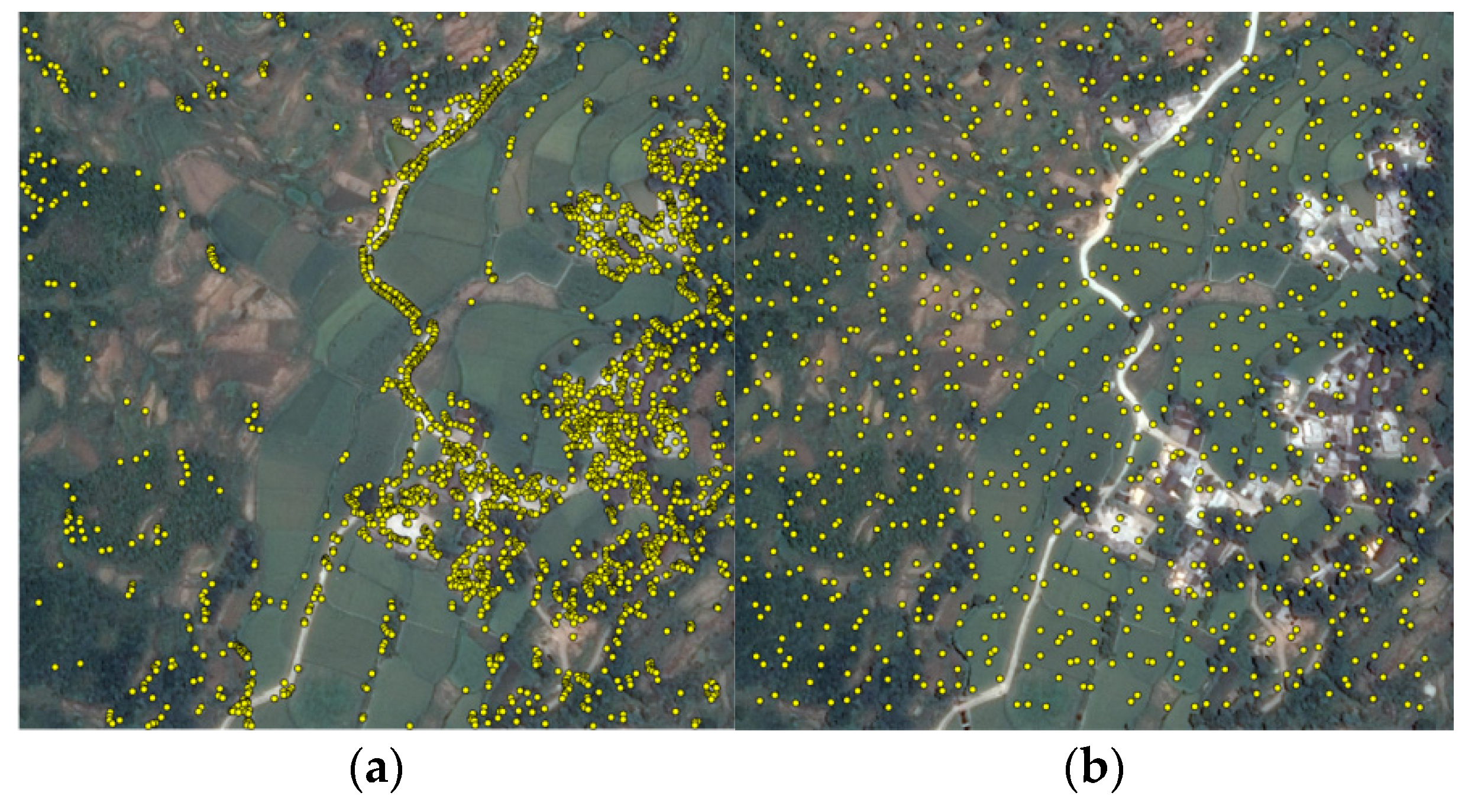
In order to detect evenly distributed interest points in the reference image, we designed a block detection strategy based on the FAST operator, which we named the block-based FAST operator. Specifically, the image was first divided into nonoverlapping blocks, and the FAST value was computed for each pixel of every block. Then, pixel points with the largest FAST values were selected as the interest points in a block. As a result, we can obtain interest points in the image, where the values of and can be decided by users. From Figure 1, it is obvious that the block-based FAST operator has a better representation than the initial one in extracting evenly distributed interest points, where and were set to 20 and 1, respectively.
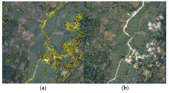
Figure 1.
Extraction results of interest points by two different strategies. (a) initial features from accelerated segment test (FAST) operator; (b) block-based FAST operator.
3.1.2. Structure Feature Extraction
Once a number of interest points are detected in the reference image, we can determine a template window centered on an interest point and predict its corresponding search window in the sensed image using the initial georeference information. Then, we can extract structure features for both the template and the search windows, before using them for correspondence detection via template matching. The selection of structural feature descriptors is crucial for image matching, and it needs to consider both robustness and computational efficiency. Accordingly, a recently published structural feature descriptor [24] named CFOG (channel features of orientated gradients) was employed for correspondence detection because it presents faster and more robust matching performance than other state-of-the-art structural feature descriptors such as HOG, LSS, and HOPC.
CFOG is built on the basis of dense orientated gradient features of images, and its construction process (see Figure 2) mainly includes two parts: orientated gradient channels and 3D Gaussian convolution. Given an image, the orientated gradient channels of the image first are calculated. Then, is used to represent each orientated gradient channel . In the actual calculation, the gradient amplitudes in the horizontal and vertical directions are used to calculate the value of each orientated gradient channel, denoted as and , respectively, which can be expressed using the following equation:
where represents the orientation of the gradient, while represents the absolute value, and its purpose is to limit the gradient direction within the range of 0° to 180°. After that, the feature channel of convolution is realized using a 3D-like Gaussian kernel.
where denotes the convolution operation, denotes the Gaussian function, and is its standard deviation. The aim of such an operation is to integrate orientated gradient information of the neighborhood for feature description, which can improve the robustness to noise and nonlinear radiometric differences.

Figure 2.
The construction process of channel features of orientated gradients (CFOG).
3.1.3. Interest Point Matching
CFOG yields the 3D pixel-wise descriptors with large data volume for both the template and the search windows. It is usually time-consuming if using these descriptors to perform the template matching with traditional similarity measures (e.g., SSD and NCC) in the spatial domain. Accordingly, we carried out the similarity evaluation in the frequency domain, where 3D PC was used as the similarity metric. Accordingly, 3D PC can effectively speed up image matching by using fast Fourier transform (FFT) because the dot product operation in the frequency domain is equal to the convolution operation in the spatial domain. The details of the matching technique are given below.
Given the CFOG descriptors of the template and search windows, their relationship is expressed as follows:
where represents the CFOG descriptors of the template window, represents the CFOG descriptors of the search window, is the offset of the two windows, and z is the dimensionality of CFOG. Let us use and to represent the corresponding and in the frequency domain. According to the translation property of Fourier transform, the corresponding relation can be expressed as
Their normalized cross-power spectrum can be expressed as
where * denotes the complex conjugate. According to the translation theory, a Dirac delta function can be obtained via the inverse Fourier transform of the normalized cross-power spectrum. The function has an obvious sharp peak value at the offset position, while the value of other positions is close to zero. Accordingly, the offset between the template and search windows can be determined by the peak position.
3.1.4. Mismatch Elimination
Due to some occlusions such as clouds and shadow, it is inevitable that some correspondences with large errors will result during the matching process. Therefore, it is necessary to eliminate these mismatches to improve the matching quality. In this paper, the random sample consensus (RANSAC) algorithm was applied to remove these outliers [51], achieving the final correspondences between the Sentinel SAR and optical images. After that, these correct correspondences were used for the subsequent analysis of geometric transformation models.
3.2. Mathematical Models of Geometric Transformation
After sufficient CPs are obtained between the Sentinel SAR and optical images, it is crucial to determine an optimum geometric transformation model for the co-registration of such images. Accordingly, we investigated several representative transformation models and analyzed their registration accuracy. These models included polynomial models, projective models, and RFMs, which are described in detail below.
3.2.1. Polynomial Models
Image correction based on polynomials does not take into account the geometric process of spatial imaging, and it deals with image deformation by means of a mathematical simulation. Geometric distortions of remote sensing images are often quite complicated because they are caused by a variety of factors such as imaging models, Earth curvature, and atmospheric refraction. In general, these distortions can be considered as the combined effect of translation, rotation, scaling, deflection, bending, affine, and higher-order deformation. It is difficult to build a rigorous mathematical model to correct these distortions, whereas an appropriate polynomial can be used to fit the geometric relationship between images. Due to their simplicity and availability, polynomials have been widely applied for image correction by many commercial software packages. Common polynomials include the first-, second-, third-, and higher-order polynomials. The general two-dimensional polynomial model is expressed as follows:
where are the coordinates of the sensed image, are the coordinates of the reference image, and are the polynomial parameters. The minimum number of correspondences for solving the parameters is related to the order of polynomials, which is calculated by
3.2.2. Projective Models
Projective transformation means that if a straight line in one image is mapped to another image, it is still a straight line, but the parallel relationship between lines cannot be maintained. The two-dimensional plane projective model is a linear transformation of homogeneous three-dimensional vectors. Under a homogeneous coordinate system, the projective transformation can be described in the following nonsingular 3 × 3 matrix form:
By setting and , Equation (9) can be rewritten as
where are the coordinates of the sensed image, and are the coordinates of the reference image.
With the development of geometric transformation models, the projective transformation can be extended by changing the properties of the same denominator and increasing the number of parameters, thus forming some flexible projective models for remote sensing image correction. These projective models are described below.
The projective model of 10 parameters is as follows:
The projective model of 22 parameters is as follows:
The projective model of 38 parameters is as follows:
where are the coordinates of the input image, are the coordinates of the reference images, and are the model parameters. The minimum number of CPs for the 10-parameter projective model is 5, that for the 22-parameter projective model is 11, and that for the 38-parameter projective model is 14.
3.2.3. RFM
Currently, the RFM is one of the commonly used geometric transformation models for remote sensing image correction. Several studies have shown that the RFM can be used as a generalized sensor model, which provides an exact approximation of rigorous sensor models for many satellite images, especially for high-resolution satellite images. This means that the RFM can replace rigorous senor models for precise geometric correction of high-resolution images. Due to its generalization, the RFM has been used as a standard data transfer format for high-resolution images. The RFM relates the object space coordinates to image space coordinates in the form of rational functions that are ratios of two polynomials. The generic form of the RFM is given as follows:
where are the coordinates in image space, are the coordinates in object space, denote the polynomials of , and their highest order is often limited to 3. In such a case, the polynomial has the following form:
where are the model parameters called rational polynomial coefficients.
The RFM has two types with the same denominator (i.e., P2 = P4) and different denominator (i.e., P2 ≠ P4). The minimum number of CPs is determined by the order of this model, which is given in Table 1. It is worth noting that the RFM is a three-dimensional polynomial model when P2 = P4 = 1.

Table 1.
Nine cases for the rational function model (RFM).
3.3. Image Co-Registration
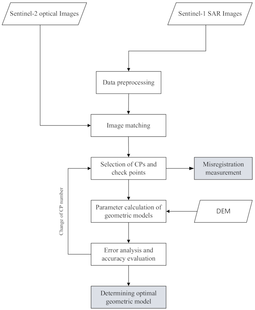
Based on the above matching approach and geometric transformation models, this paper proposes a technical solution to measure the misregistration shifts and improve the co-registration accuracy between the Sentinel SAR and optical images. Figure 3 shows the technique flowchart.

Figure 3.
Flowchart of misregistration measurement and improvement for the Sentinel-1 Synthetic Aperture Radar (SAR) and the Sentinel-2 optical images.
3.3.1. Data Preprocessing
According to the data description in Section 2, the Sentinel-1 SAR L1 images and Sentinel-2 optical L1C images have different projection coordinate systems and different sizes. Accordingly, a reprojection and a crop operation are carried out for the two types of images before co-registration. In this study, the SAR images were reprojected into the coordinate system (i.e., UTM and WGS84) of the optical images. Considering that the SAR images have some geolocation errors, and their sizes are larger than the optical images, we cropped the SAR images by using the geographical range of the optical images with adding some margin (e.g., 100 pixels) in each direction. Such a process ensured that the two types of images could cover the same geographical range.
3.3.2. Image Matching
We detected sufficient and evenly distributed correspondences between images using the technique described in Section 3.1. Some of these correspondences were selected as CPs which were used to calculate the parameters of geometric transformation models, while others were used as checkpoints to evaluate the registration accuracy of these models.
3.3.3. Misregistration Measurement
The correspondences between the Sentinel SAR and optical images should have the same geographical coordinates if the two types of images are co-registered exactly. According to this precondition, the differences in geographical coordinates of the correspondences correspond to the misregistration shifts between the Sentinel SAR and optical images. Accordingly, the misregistration shift is quantified as follows:
where , and , are the matched location for correspondence between the Sentinel SAR and optical images, are the misregistration shifts (units: 10 m pixels) in the and directions for one correspondence, and are the mean misregistration shifts in the and directions. is the mean misregistration shift between the SAR and optical images, and there are a total of correspondences.
3.3.4. Parameter Calculation of Geometric Models
Using the obtained CPs, we calculated the parameters of the employed geometric models including polynomial models, projective models, and RFMs using the least square method. Meanwhile, the digital elevation model (DEM) was introduced for the parameter calculation of RFMs.
3.3.5. Accuracy Analysis and Evolution
We adjusted the number of CPs to perform the registration experiment, and then computed the root-mean-square errors (RMSEs, Equation (27)) of checkpoints for accuracy evaluation of each geometric model. Lastly, the optimal geometric model was determined for the co-registration of the SAR and optical images.
where denotes the geometric transformation model, and is the number of checkpoints.
4. Experiments
4.1. Experimental Data
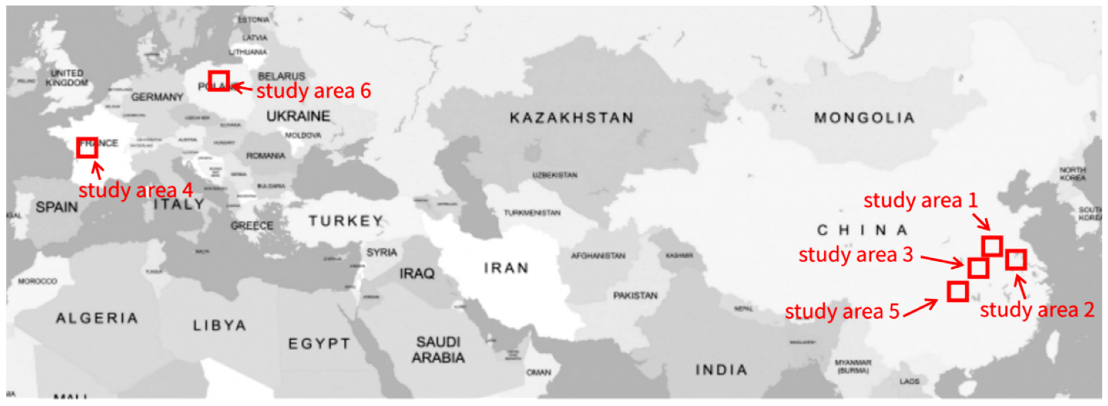
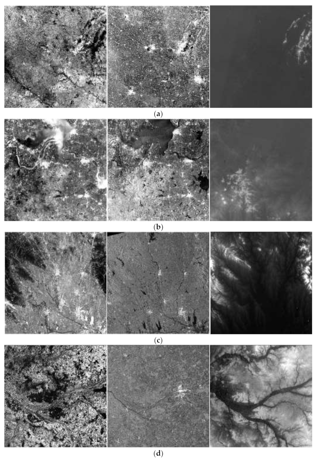
We selected six pairs of Sentinel-1 SAR L1 images and Sentinel-2 optical L1C images for the experiment. These images were located in China and Europe (see Figure 4) and covered three types of different terrains: flat areas, hilly areas, and mountainous areas. Each type included two pairs of images. These images were almost cloud-free, which makes the applied matching technique reliable to detect correspondences between such images. Table 2 gives the detail description of the experimental data. In addition, the 30 m DEM data were obtained from Advanced Spaceborne Thermal Emission and Reflection Radiometer DEM (ASTER GDEM), and were used as the elevation reference data for image correction. All these experimental data are shown in Figure 5.

Figure 4.
Study areas in China and Europe.

Table 2.
Detailed description of experimental data.

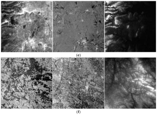
Figure 5.
Experimental data including optical images (left), SAR images (middle), and DEMs (right): (a) study area 1; (b) study area 2; (c) study area 3; (d) study area 4; (e) study area 5; (f) study area 6.
4.2. Image Matching
For image matching, the optical image was first divided into 20 × 20 girds and one FAST interest point was detected in each grid, reaching a total of 400 interest points. Then, their match points in the SAR image were determined by using CFOG and 3D PC via template matching, where the template window was set to 100 × 100 pixels, and the search window was set to 200 × 200 pixels. Lastly, the RANSAC algorithm was employed to remove the outliers to obtain the correspondences. The matching process was performed on a personal computer (PC) with an Intel Core i7-10700KF central processing unit (CPU) 3.80 GHz. Table 3 shows the number of interest points, the correspondences, and the run time. It can be found that these image pairs achieved different numbers of correspondences because of their different image characteristics. Specifically, the images covering flat areas obtained more correspondences than the images covering mountain areas. This may be attributed to the images of mountain areas having more significant local geometric distortions than flat areas. These geometric distortions resulted in the extracted structural features between the images not corresponding well, which degraded the matching performance to some degree. In addition, the run time was about 6.6 s for all the image pairs, which demonstrated the high computational efficiency of the proposed match method. Overall, our match approach was fast and reliable for the matching of the Sentinel SAR and optical images, and the obtained correspondences for all the tested image pairs were sufficient for their co-registration. To make a fair and reasonable test, it is necessary to use the same number of correspondences to perform the following misregistration measurement and compare the registration accuracy of different transformation models. Accordingly, we selected 143 correspondences with the fewest residuals for each image pair in the subsequent tests.

Table 3.
Matching statistics of all study areas.
4.3. Misregistration Measurement
According to the 143 obtained correspondences in the previous subsection, we used their mean offsets of match locations to compute the misregistration shifts , , and (see Equation (21)–(26)). Figure 6 shows the misregistration shifts of the six pairs of images covering three different terrains. In general, the misregistration shifts presented a large difference for different terrains. The misregistration shifts were kept at about 20–30 pixels in the flat areas and about 20–40 pixels in hilly areas, respectively. On the other hand, in the mountainous areas with large topographic relief, the misregistration shifts increased sharply to about 50–60 pixels. This is because the Sentinel SAR and optical images had different imaging geometry models, whereby the SAR sensor acquired data in a side-looking geometry while the optical sensor captured data via push-broom imaging. This increased the geometric distortions between them with the increase in terrain fluctuation.
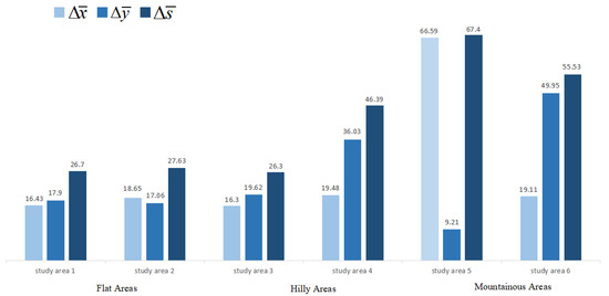
Figure 6.
Statistics of mean misregistration shifts (units: pixels) of correspondences for different terrains.
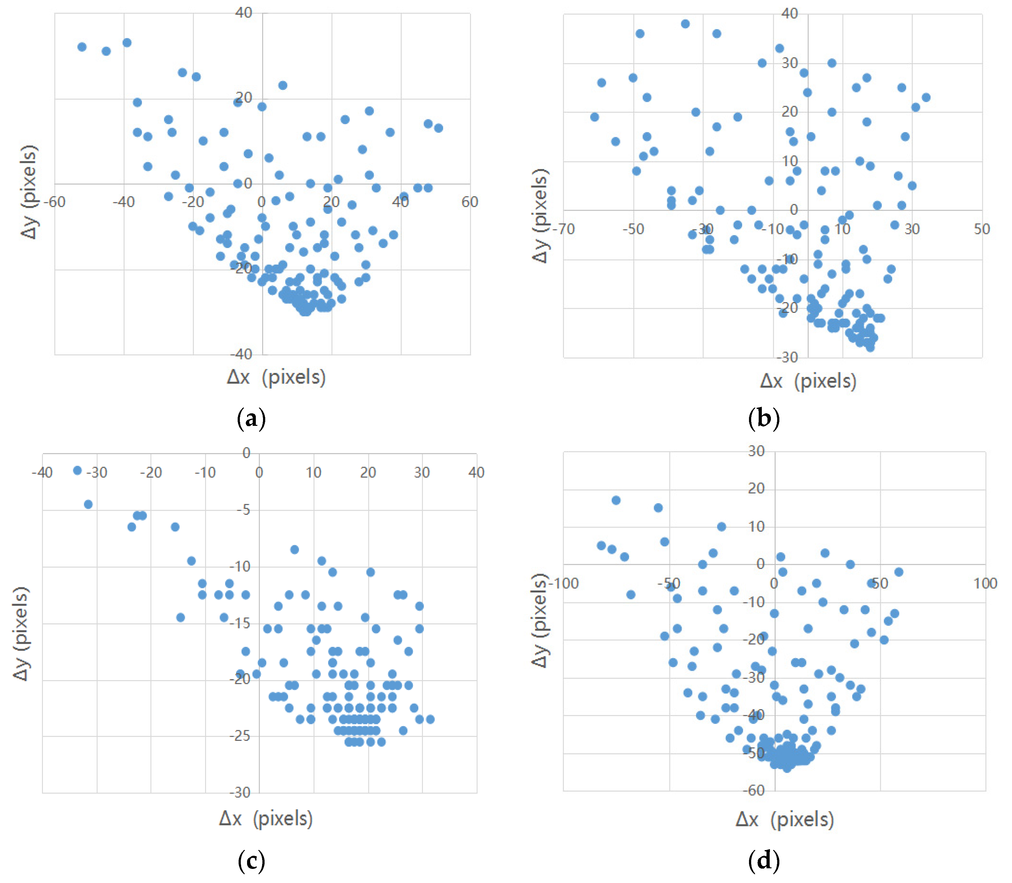
Table 4 gives the statistics of the misregistration shifts for each image pair. We can see that all these images pairs had large standard deviations (STDs), which means that the misregistration shifts were unevenly distributed across the images; that is, the misregistration shifts were quite different for the correspondences in different regions of each image pair (see Figure 7). The results indicate that these images have significant nonlinear geometric distortions, and different image regions correspond to different misregistration shifts. The main reason is that the Sentinel-1 SAR images did not undergo terrain correction.

Table 4.
Statistics of the misregistration shifts (units: pixels) of all the study areas.
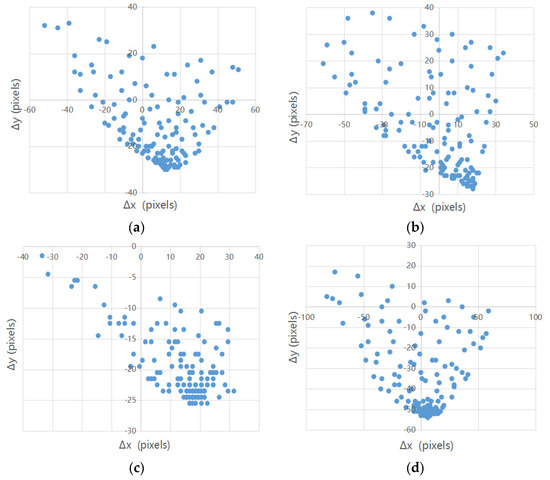
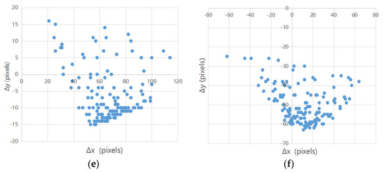
Figure 7.
Distribution of misregistration shifts (units pixels) and of different correspondences for all the study areas: (a) study area 1; (b) study area 2; (c) study area 3; (d) study area 4; (e) study area 5; (f) study area 6.
The above results demonstrate that there are evident misregistration shifts between the Sentinel-1 SAR and Sentinel-2 optical images. Accordingly, a further co-registration process for the SAR and optical images is presented below.
4.4. Co-Registration Accuracy Analysis and Evaluation
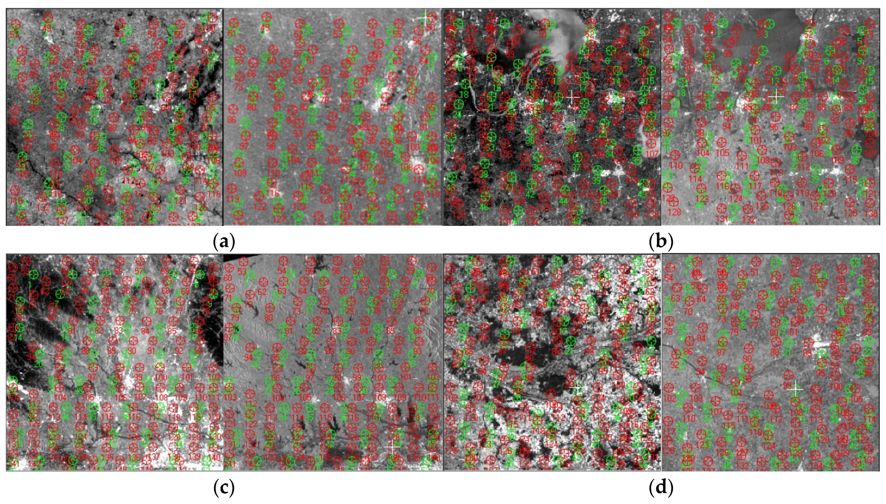
In this subsection, we evaluate the registration accuracy of different geometric transformation models for the Sentinel-1 SAR and Sentinel-2 optical images. Firstly, the obtained 143 correspondences (in Section 4.2) were divided into checkpoints and CPs (see Figure 8), where 48 correspondences were used as checkpoints and the others were used as CPs (their number is variable). Then, we compared the performance of the polynomials (from first up to fifth order), the projective transformations (for 10 parameters up to 38 parameters), and the RFMs (from first up to third) under different numbers of CPs (from 25 to 95) and different terrains. Lastly, an optimum geometric model was determined for the co-registration of the two types of images. The experimental analysis for different terrains is given below.
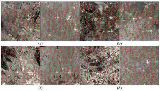

Figure 8.
Control points (CPs) (red) and checkpoints (green) for optical (left) and SAR (right) images: (a) study area 1; (b) study area 2; (c) study area 3; (d) study area 4; (e) study area 5; (f) study area 6.
4.4.1. Accuracy Analysis of Flat Areas
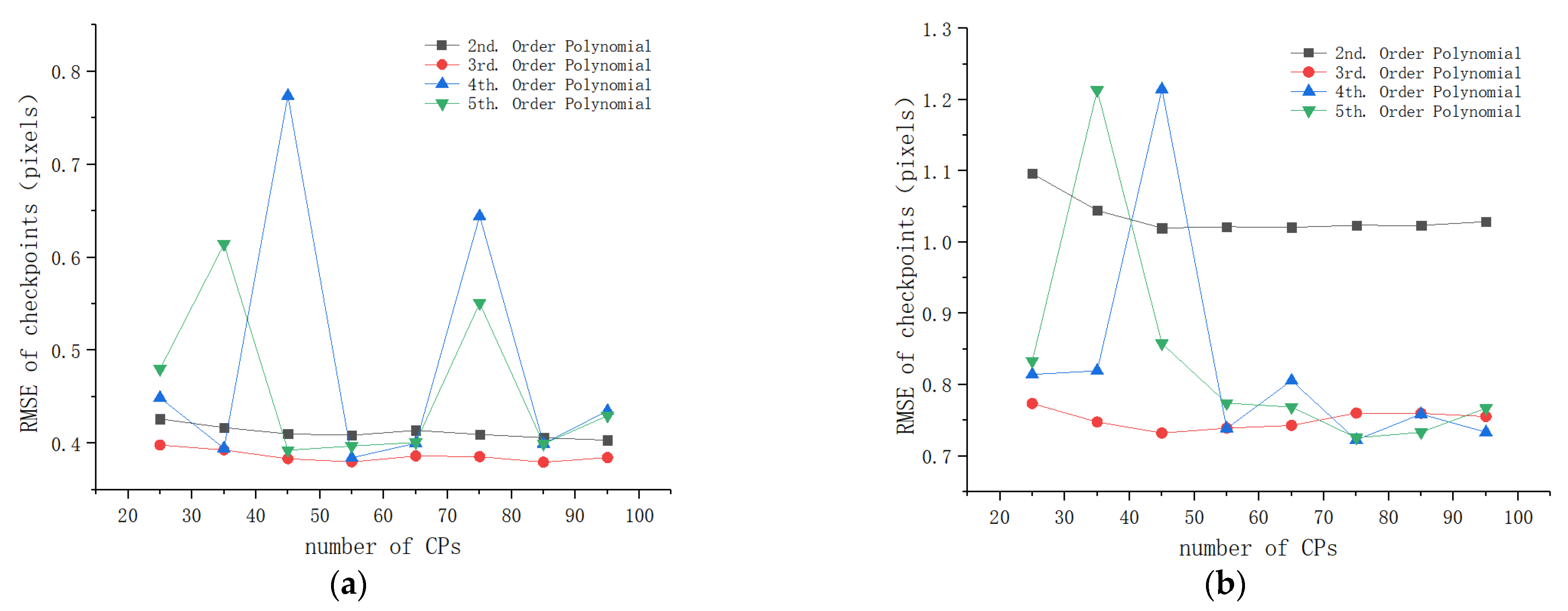
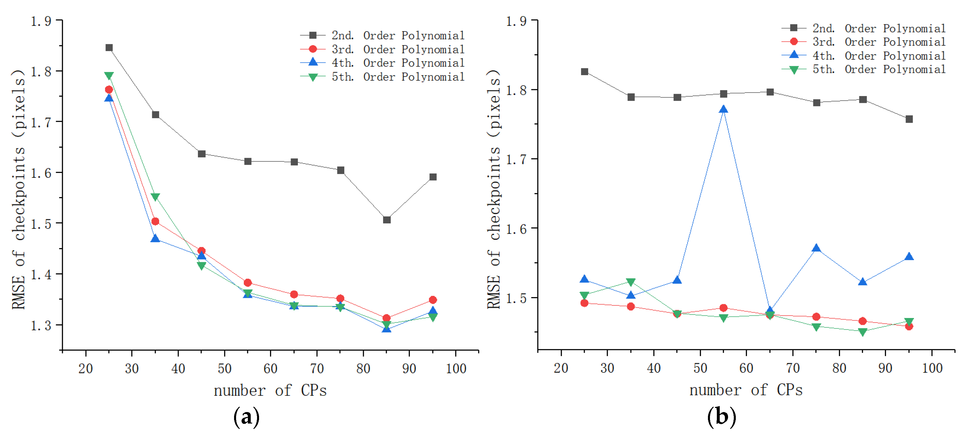
Let us first analyze the registration accuracy of the polynomial models. It can be found from Table 5 that the RMSEs of the first-order polynomial were more than 10 pixels for the two flat areas, which are much larger than these of the other polynomials. Accordingly, we mainly compared the registration accuracy of the polynomials (from second- to fifth-order) because their RMSEs were relatively close. Figure 9 shows the checkpoint RMSEs versus the number of CPs for these polynomials. It can be observed that the second-order and the third-order polynomials presented a stable performance when the number of CPs changed. The third-order polynomial achieved higher registration accuracy than the second-order polynomial, and its accuracy was kept at about 0.4 pixels for study area 1 and about 0.75 pixels for study area 2. For the fourth-order and fifth-order polynomials, although their accuracy was close to that of the third-order polynomial under a large number of control points (e.g., more than 80), their performance had a significant fluctuation with the change in the number of CPs. Moreover, they required more CPs for image registration compared with the third-order polynomial, which would increase computational cost and is not beneficial to practical application. According to the above analysis, the third-order polynomial performed better compared with the other polynomials.

Table 5.
Checkpoint error statistics (units: pixels) of different geometric models in the flat areas, where the number of CPs was 95 and the number of checkpoints was 48. RMSE, root-mean-square error.
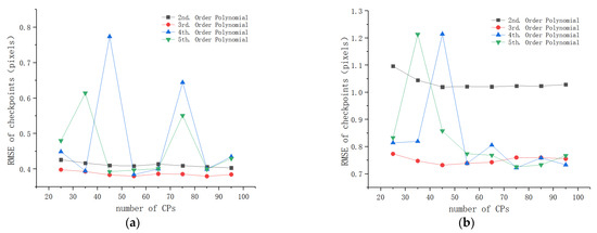
Figure 9.
Checkpoint RMSEs of polynomials for the flat areas: (a) study area 1; (b) study area 2.
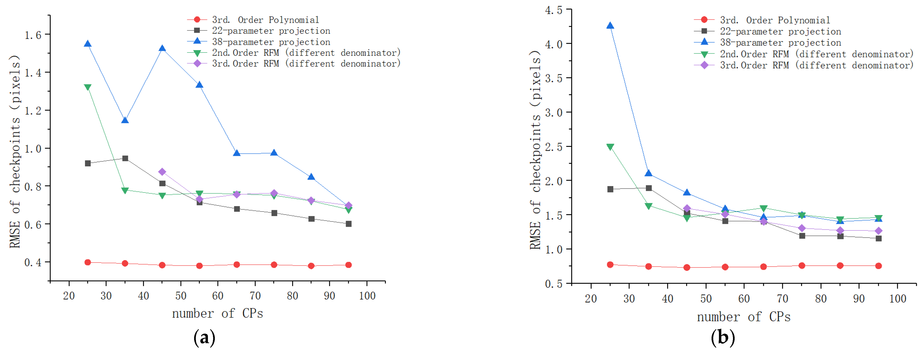
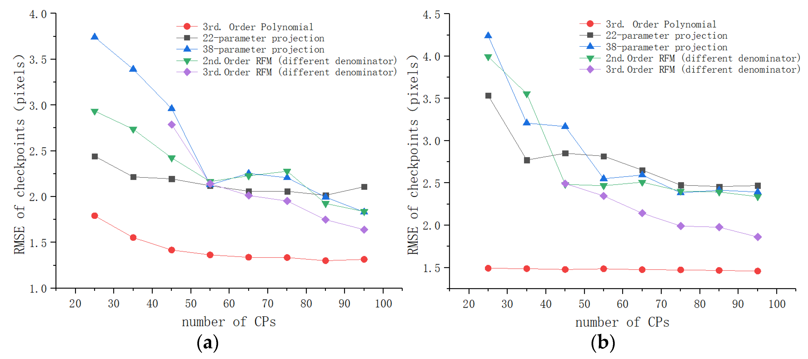
For projective models and RFMs, we can see from Table 5 that the 22-parameter and 38-parameter projective models performed better than the other projective models, and the second-order and third-order RFMs (different denominator) achieved higher accuracy than the others. Accordingly, these models were compared with the third-order polynomial. Figure 10 shows their checkpoint RMSEs versus the number of CPs. It can be clearly observed that the third-order polynomial achieved the smallest RMSEs under any number of CPs among these models. Moreover, the performance of the third-order polynomial was more stable than that of the other models when the number of CPs changed. These results demonstrate that the third-order polynomial was the best geometric transformation model for the co-registration of the Sentinel-1 SAR and Sentinel-2 optical images in flat areas.
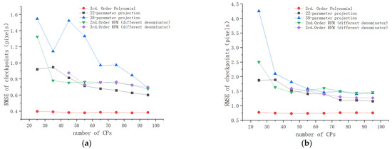
Figure 10.
Checkpoint RMSEs of the third-order polynomial and other geometric models for the flat areas: (a) study area 1; (b) study area 2.
4.4.2. Accuracy Analysis of Hilly Areas
The experimental analysis was similar to that in the flat areas. We also first compared and analyzed the registration accuracy of the polynomials. From Table 6, we can see that the first-order polynomial performed much worse than the other polynomials. Accordingly, the comparative analysis focuses on the polynomials of second-order to fifth-order. Figure 11 shows the checkpoint RMSEs versus the number of CPs for these polynomials. It can be seen that the second-order polynomial obtained lower accuracy than the other polynomials, while the third-order, the fourth-order, and the fifth-order polynomials achieved similar accuracy. However, in study area 4, the accuracy of the fourth-order polynomial had a sharp fluctuation when the number of CPs changed (see Figure 11b), which shows its instability for image registration. The third-order and the fifth-order polynomials presented a stable performance and had the same level of accuracy, but the third-order polynomial required fewer CPs and was more computationally efficient than the fifth-order polynomial. Accordingly, the third-order polynomial was more preferable than the other polynomials.

Table 6.
Checkpoint error statistics (units: pixels) of different geometric models in the hilly area, where the number of CPs was 95 and the number of checkpoints was 48.
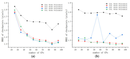
Figure 11.
Checkpoint RMSEs of polynomials for the flat areas: (a) study area 3; (b) study area 4.
For the other geometric models, those with higher accuracy were selected to compare with the third-order polynomial. We can see from Table 6 that these models were the 22-parameter projective transformation, the 38-paremeter projective transformation, and the second-order and the third-order RFMs (different denominator). Figure 12 shows the checkpoint RMSEs versus the number of CPs for these models. Apparently, the third-order polynomial achieved a registration accuracy of about 1.5 pixels for both study area 3 and study area 4, and it outperformed the other models under any number of CPs. These results confirm that the third-order polynomial was optimal among these models for the co-registration of the Sentinel-1 SAR and Sentinel-2 optical images in hilly areas.
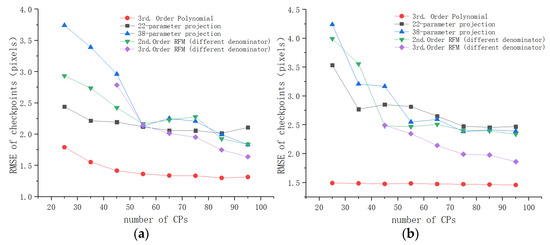
Figure 12.
Checkpoint RMSEs of the third-order polynomial and the other geometric models for hilly areas: (a) study area 3; (b) study area 4.
4.4.3. Accuracy Analysis of Mountainous Areas
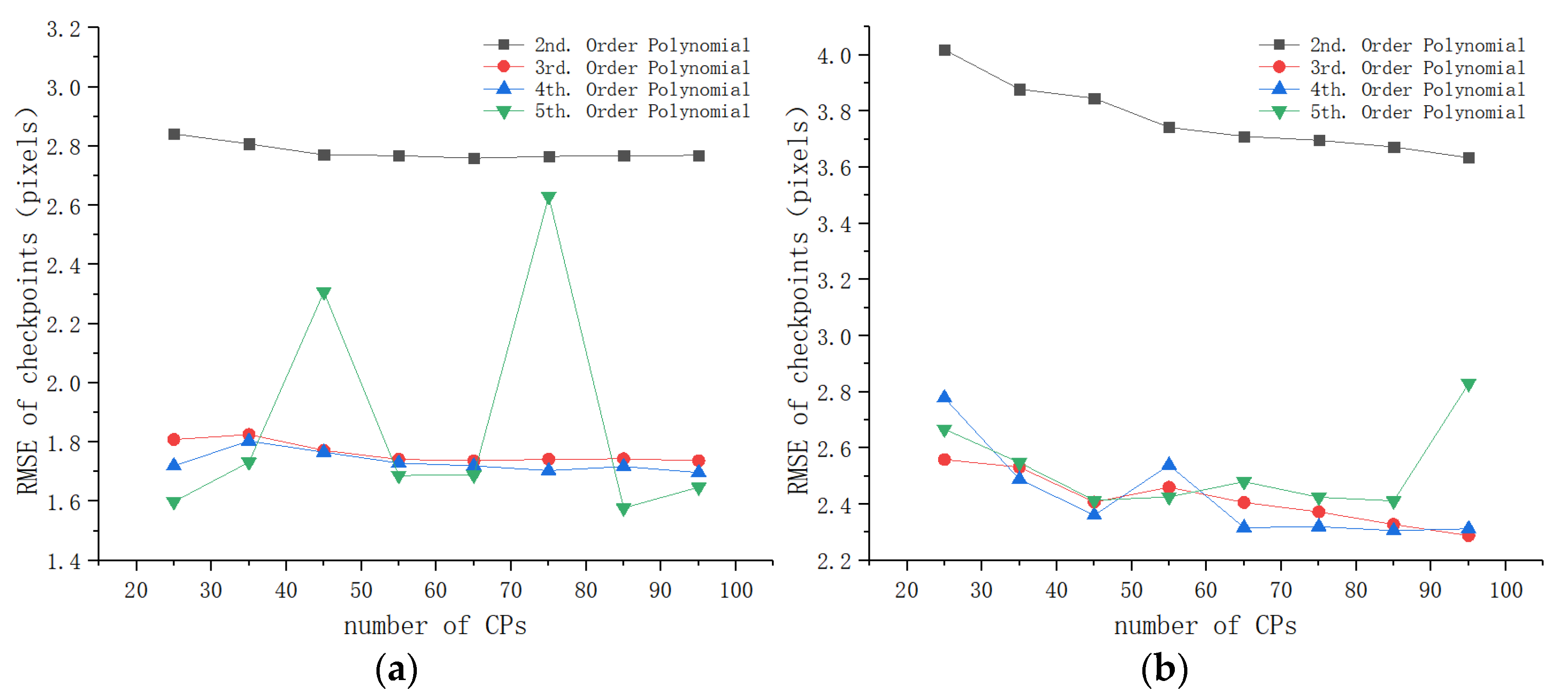
Figure 13 shows the checkpoint RMSEs versus the number of CPs for the polynomials. We can see that the second-order polynomial performed much worse than the other polynomials. The accuracy of the fifth-order polynomial had a significant fluctuation when the number of control points changed. By comparison, the third-order and the fourth-order polynomials had a more stable performance and achieved higher accuracy. Compared to the fourth-order polynomial, the performance of the third-order polynomial was more stable for study area 6, and it required fewer CPs. Accordingly, the third-order polynomial was more suitable than the other polynomials for the co-registration of these images.
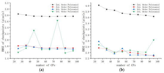
Figure 13.
Checkpoint RMSEs of the polynomials for the mountainous areas: (a) study area 5; (b) study area 6.
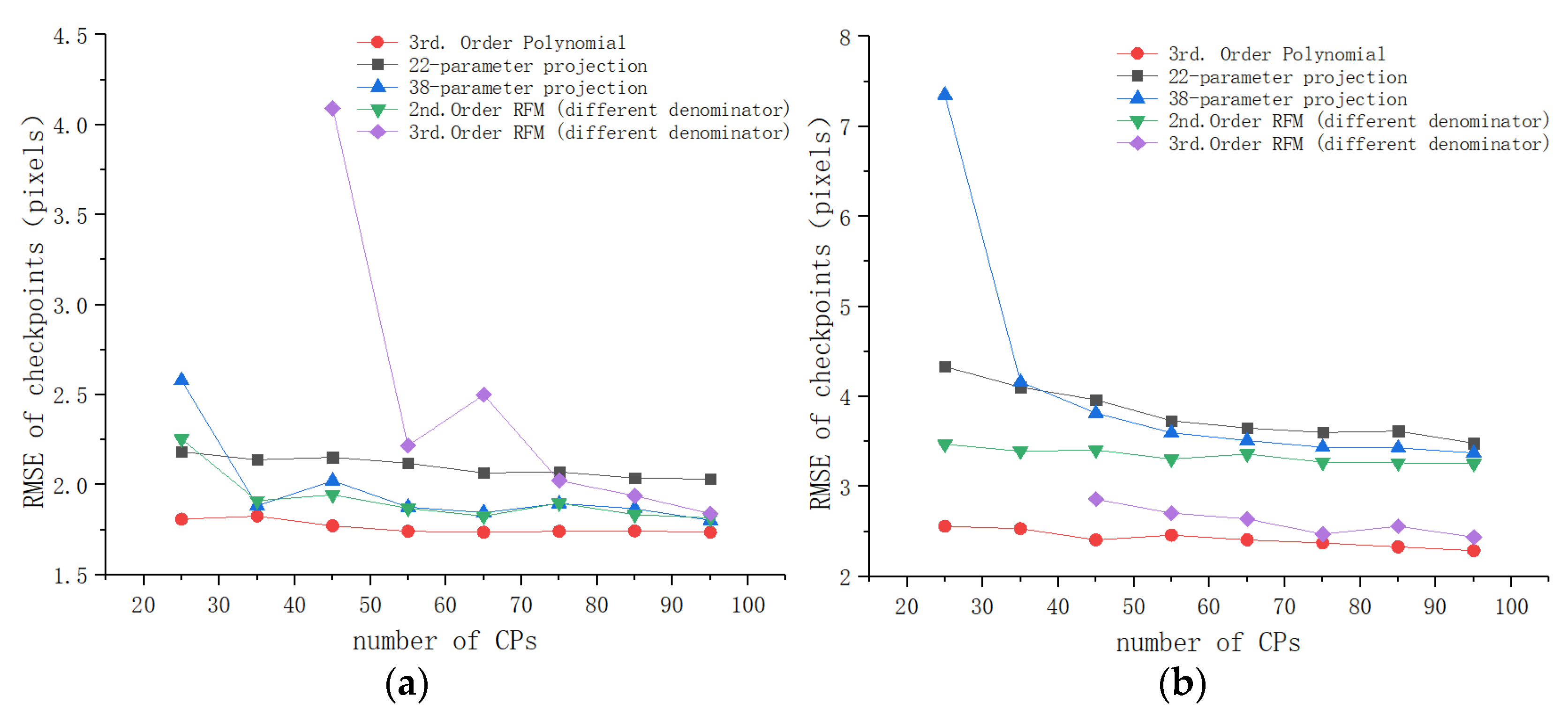
As with the analysis scheme in flat and hilly areas, we chose several other models with higher accuracy from Table 7, and we compared them with the third-order polynomial. Figure 14 shows the checkpoint RMSEs versus the number of CPs for these models. For study area 5, the accuracy of the third-order polynomial was about 1.7 pixels, which is much better than that of the other models. In the case of study area 6, the accuracy of the third-order RFM model improved with the increase in the number of CPs, and its accuracy was close to that of the third-order polynomial when the number of CPs reached 95. However, the third-order polynomial still yielded slightly better accuracy than the third-order RFM model. The accuracy was about 2.3 pixels. Furthermore, the third-order polynomial required fewer control points compared with the third-order RFM model. Therefore, the third-order polynomial outperformed the other geometric transformation models for the co-registration of the Sentinel-1 SAR and Sentinel-1 optical images in mountainous areas.

Table 7.
Checkpoint error statistics (units: pixels) of different geometric models in mountainous areas, where the number of CPs was 95 and the number of checkpoints was 48.
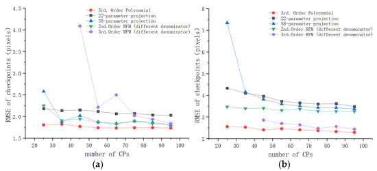
Figure 14.
Checkpoint RMSEs of the third-order polynomial and the other geometric models for mountainous areas: (a) study area 5; (b) study area 6.
4.4.4. Evaluation of Registration Results
According to the above experimental analysis, the third-order polynomial was the optimal geometric transformation model for the co-registration of the Sentinel-1 SAR and Sentinel-2 optical images; thus, this model was used to perform the image registration. This process took about 3 s for one image pair using our PC. Since the previous image matching process took about 6.7 s, the proposed method took less than 10 s to complete the whole co-registration.
To illustrate the advantage of the proposed method, it was compared with the terrain correction process using the SNAP toolbox. Table 8 gives the registration accuracy and run time of the two methods. We can see that the proposed method outperformed the terrain correction process for most test cases in terms of registration accuracy, especially for the images covering flat and hilly areas. Moreover, the proposed method was almost 100 times faster than the terrain correction process, which is quite beneficial for the response to emergency events such as earthquakes and floods. The registration results are shown in Figure 15. It can be observed that the Sentinel-1 SAR and Sentinel-2 optical images aligned well.

Table 8.
Comparison of registration results of the proposed method and the terrain correction process.

Figure 15.
Examples of Sentinel-1 SAR and Sentinel-2 optical image registration: (a) study area 1; (b) study area 2; (c) study area 3; (d) study area 4; (e) study area 5; (f) study area 6.
5. Discussion and Conclusions
This paper first proposed a fast and robust block-based match scheme using structural features and 3D PC for correspondence detection between the Sentinel-1 SAR L1 IW GRD 10 m images and the Sentinel-2 optical L1C 10 m images. Then, the obtained correspondences were used to measure the misregistration shifts of the two types of images and analyze the performance of various geometric transformation models for their co-registration. Lastly, an optimal geometric model was determined to improve the registration accuracy.
For image matching, we applied various techniques to ensure the matching quality. The block-based scheme is aimed at evenly distributing the correspondences over the images, the CFOG structural feature descriptor can handle significant radiometric differences between the images, and 3D PC greatly improves the computational efficiency. The mismatches were removed using the RANSAC algorithm. Accordingly, the obtained correspondences were reliable for misregistration measurement and the accuracy evaluation of geometric transformation models.
The misregistration was measured by computing the geometric shifts of correspondences between the two types of images. Six pairs of images covering different terrains were matched and used for the misregistration measurement, as well as for the subsequent co-registration tests. Experimental results showed that the misregistration shifts between them were between 20 and 60 10 m pixels, and the shifts varied drastically in different regions of images. Furthermore, the misregistration increased with the increase in topographic relief. Specifically, the misregistration of the flat areas was kept at 20–30 10 m pixels, that of the hilly areas was kept at 20–40 10 m pixels, and that of the mountainous areas increased to 50–60 10 m pixels. Such large registration shifts resulted in the two types of images not being effectively integrated for subsequent remote sensing applications without a precise co-registration. Since only six pairs of images were used to measure the misregistration shifts, the shifts may be different when using images located in other areas and acquired at other times. However, this research found that misregistration shifts are common between the Sentinel-1 SAR L1 and Sentinel-2 optical L1C images. Moreover, a larger topographic relief leads to larger misregistration shifts.
To improve the co-registration accuracy between the Sentinel-1 SAR and Sentinel-2 optical images, we compared the performance of a variety of geometric transformation models including polynomials, projective models, and RFMs. In general, considering some factors such as registration accuracy, required number of CPs, and stability of performance, the third-order polynomial performed better than the other models, while the projective models did not achieve satisfactory registration accuracy. For the RFMs, especially the third-order RFM, although they consider the influence of terrain height and are widely used for the correction and registration of high-resolution images, their performance was not quite satisfactory for the co-registration of the Sentinel SAR and optical images. The main reason may be that the parameters of the RFMs were calculated using numerous CPs in the case of high-resolution images [31]. On the other hand, in our experiments, the number of CPs was limited within 95, which may not have been able to provide the exact solution for the RFM parameters. Accordingly, the accuracy of the RFMs could be improved by increasing the number of CPs. In summary, our experiments showed that the third-order polynomial is the optimal geometrical model under a limited number of CPs (e.g., fewer than 95) for the co-registration of Sentinel-1 SAR and Sentinel-2 optical images.
Compared with the co-registration process pipeline where the terrain correction is applied to the Sentinel-1 SAR images using the SNAP toolbox, the proposed method is almost 100 times faster, and it obtains higher registration accuracy for most tested image pairs, especially for images covering flat and hilly areas. Therefore, the proposed method can effectively improve the co-registration for Sentinel SAR and optical images, while also meeting the requirements of real-time processing. In addition, the registration accuracy of the proposed method varied for different terrains. When using the optimal geometric model (i.e., the third-order polynomial), The flat areas achieved the highest accuracy, reaching the sub-pixel level (approximately 0.4 to 0.75 pixels), followed by the hilly areas which achieved an accuracy of about 1.5 pixels, whereas the mountainous areas had the lowest accuracy between 1.7 and 2.3 pixels. These results illustrate that the registration accuracy decreased with the increase in topographic relief. This is because large topographic relief increases local geometric distortions between images, and the third-order polynomial can only approximately fit these distortions. To track this problem, a possible solution is to perform a true ortho-rectification using the rigorous physical models and orbit ephemeris parameters of Sentinel-1 and Sentinel-2 satellites. Meanwhile, high-resolution DEM data should also be used in this process. These studies will be carried out in future research. Moreover, we will also test some nonrigid geometric transformation models such as the piecewise linear and thin plate spline functions for the co-registration of Sentinel-1 SAR and Sentinel-2 optical images.
Author Contributions
Y.Y., C.Y. and L.Z. developed the method and wrote the manuscript. B.Z., Y.H. and H.J. designed and carried out the experiments. All authors analyzed the results and improved the manuscript. All authors have read and agreed to the published version of the manuscript.
Funding
This paper was supported by the National Natural Science Foundation of China (No.41971281) and the Sichuan Science and Technology Program (No. 2020JDTD0003).
Institutional Review Board Statement
Not applicable.
Informed Consent Statement
Not applicable.
Data Availability Statement
The publicly available datasets were used in this study. The Sentinel-1 SAR and Sentinel-1 optical images can be downloaded from here: [https://scihub.copernicus.eu/ (accessed on 1 January 2021)].
Conflicts of Interest
The authors declare no conflict of interest.
References
- Scarpa, G.; Gargiulo, M.; Mazza, A.; Gaetano, R. A CNN-Based Fusion Method for Feature Extraction from Sentinel Data. Remote Sens. 2018, 10, 236. [Google Scholar] [CrossRef]
- Haas, J.; Ban, Y. Sentinel-1A SAR and sentinel-2A MSI data fusion for urban ecosystem service mapping. Remote Sens. Appl. Soc. Environ. 2017, 8, 41–53. [Google Scholar] [CrossRef]
- He, W.; Yokoya, N. Multi-Temporal Sentinel-1 and -2 Data Fusion for Optical Image Simulation. ISPRS Int. J. Geo Inf. 2018, 7, 389. [Google Scholar] [CrossRef]
- Meraner, A.; Ebel, P.; Zhu, X.X.; Schmitt, M. Cloud removal in Sentinel-2 imagery using a deep residual neural network and SAR-optical data fusion. ISPRS J. Photogramm. Remote Sens. 2020, 166, 333–346. [Google Scholar] [CrossRef]
- Urban, M.; Berger, C.; Mudau, T.; Heckel, K.; Truckenbrodt, J.; Onyango Odipo, V.; Smit, I.; Schmullius, C. Surface Moisture and Vegetation Cover Analysis for Drought Monitoring in the Southern Kruger National Park Using Sentinel-1, Sentinel-2, and Landsat-8. Remote Sens. 2018, 10, 1482. [Google Scholar] [CrossRef]
- Chang, J.; Shoshany, M. Mediterranean shrublands biomass estimation using Sentinel-1 and Sentinel-2. In Proceedings of the 2016 IEEE International Geoscience and Remote Sensing Symposium (IGARSS), Beijing, China, 10–15 June 2016; pp. 5300–5303. [Google Scholar]
- Clerici, N.; Valbuena Calderón, C.A.; Posada, J.M. Fusion of Sentinel-1A and Sentinel-2A data for land cover mapping: A case study in the lower Magdalena region, Colombia. J. Maps 2017, 13, 718–726. [Google Scholar] [CrossRef]
- Whyte, A.; Ferentinos, K.P.; Petropoulos, G.P. A new synergistic approach for monitoring wetlands using Sentinels -1 and 2 data with object-based machine learning algorithms. Environ. Model. Softw. 2018, 104, 40–54. [Google Scholar] [CrossRef]
- Ye, Y.; Shan, J. A local descriptor based registration method for multispectral remote sensing images with non-linear intensity differences. ISPRS J. Photogramm. Remote Sens. 2014, 90, 83–95. [Google Scholar] [CrossRef]
- Zitová, B.; Flusser, J. Image registration methods: A survey. Image Vis. Comput. 2003, 21, 977–1000. [Google Scholar] [CrossRef]
- Harris, C.; Stephens, M. A Combined Edge and Corner Detector. In Proceedings of the fourth Alvey Vision Conference (ACV88), Manchester, UK, September 1988; pp. 147–152. [Google Scholar]
- Lowe, D.G. Distinctive Image Features from Scale-Invariant Keypoints. Int. J. Comput. Vis. 2004, 60, 91–110. [Google Scholar] [CrossRef]
- Bay, H.; Ess, A.; Tuytelaars, T.; Van Gool, L. Speeded-Up Robust Features (SURF). Comput. Vis. Image Underst. 2008, 110, 346–359. [Google Scholar] [CrossRef]
- Sedaghat, A.; Ebadi, H. Remote Sensing Image Matching Based on Adaptive Binning SIFT Descriptor. IEEE Trans. Geosci. Remote Sens. 2015, 53, 5283–5293. [Google Scholar] [CrossRef]
- Bouchiha, R.; Besbes, K. Automatic Remote-sensing Image Registration Using SURF. Int. J. Comput. Theory Eng. 2013, 5, 88–92. [Google Scholar] [CrossRef]
- Fan, J.; Wu, Y.; Li, M.; Liang, W.; Cao, Y. SAR and Optical Image Registration Using Nonlinear Diffusion and Phase Congruency Structural Descriptor. IEEE Trans. Geosci. Remote Sens. 2018, 56, 5368–5379. [Google Scholar] [CrossRef]
- Hel-Or, Y.; Hel-Or, H.; David, E. Matching by Tone Mapping: Photometric Invariant Template Matching. IEEE Trans. Pattern Anal. Mach. Intell. 2014, 36, 317–330. [Google Scholar] [CrossRef]
- Suri, S.; Reinartz, P. Mutual-Information-Based Registration of TerraSAR-X and Ikonos Imagery in Urban Areas. IEEE Trans. Geosci. Remote Sens. 2010, 48, 939–949. [Google Scholar] [CrossRef]
- Dalal, N.; Triggs, B. Histograms of Oriented Gradients for Human Detection. In Proceedings of the 2005 IEEE Computer Society Conference on Computer Vision and Pattern Recognition (CVPR’05), San Diego, CA, USA, 20–25 June 2005; pp. 886–893. [Google Scholar]
- Shechtman, E.; Irani, M. Matching Local Self-Similarities across Images and Videos. In Proceedings of the 2007 IEEE Conference on Computer Vision and Pattern Recognition, Minneapolis, MN, USA, 17–27 June 2007; pp. 1–8. [Google Scholar]
- Ye, Y.; Shan, J.; Bruzzone, L.; Shen, L. Robust Registration of Multimodal Remote Sensing Images Based on Structural Similarity. IEEE Trans. Geosci. Remote Sens. 2017, 55, 2941–2958. [Google Scholar] [CrossRef]
- Yan, X.; Zhang, Y.; Zhang, D.; Hou, N. Multimodal image registration using histogram of oriented gradient distance and data-driven grey wolf optimizer. Neurocomputing 2020, 392, 108–120. [Google Scholar] [CrossRef]
- Ye, Y.; Shen, L.; Hao, M.; Wang, J.; Xu, Z. Robust Optical-to-SAR Image Matching Based on Shape Properties. IEEE Geosci. Remote Sens. Lett. 2017, 14, 564–568. [Google Scholar] [CrossRef]
- Ye, Y.; Bruzzone, L.; Shan, J.; Bovolo, F.; Zhu, Q. Fast and Robust Matching for Multimodal Remote Sensing Image Registration. IEEE Trans. Geosci. Remote Sens. 2019, 57, 9059–9070. [Google Scholar] [CrossRef]
- El-Manadili, Y.; Novak, K. Precision rectification of SPOT imagery using the Direct Linear Transformation model. Photogramm. Eng. Remote Sens. 1996, 62, 67–72. [Google Scholar]
- Okamoto, A. An alternative approach to the triangulation of spot imagery. Int. Arch. Photogramm. Remote Sens. 1998, 32, 457–462. [Google Scholar]
- Smith, D.P.; Atkinson, S.F. Accuracy of rectification using topographic map versus GPS ground control points. Photogramm. Eng. Remote Sens. 2001, 67, 565–570. [Google Scholar]
- Gao, J. Non-differential GPS as an alternative source of planimetric control for rectifying satellite imagery. Photogramm. Eng. Remote Sens. 2001, 67, 49–55. [Google Scholar]
- Shaker, A.; Shi, W.; Barakat, H. Assessment of the rectification accuracy of IKONOS imagery based on two-dimensional models. Int. J. Remote Sens. 2005, 26, 719–731. [Google Scholar] [CrossRef]
- Dowman, L.; Dolloff, J.T. An evaluation of relational functions for photogrammetric restitution. Int. Arch. Photogramm. Remote Sens. 2000, 33, 254–266. [Google Scholar]
- Tao, C.V.; Hu, Y. A comprehensive study of the rational function model for photogrammetric processing. Photogramm. Eng. Remote Sens. 2001, 67, 1347–1357. [Google Scholar]
- Tao, C.V.; Hu, Y. 3D reconstruction methods based on the rational function model. Photogramm. Eng. Remote Sens. 2002, 68, 705–714. [Google Scholar]
- Hu, Y.; Tao, C.V. Updating solutions of the rational function model using additional control information. Photogramm. Eng. Remote Sens. 2002, 68, 715–723. [Google Scholar]
- Fraser, C.; Baltsavias, E.; Gruen, A. Processing of Ikonos imagery for submetre 3D positioning and building extraction. ISPRS J. Photogramm. Remote Sens. 2002, 56, 177–194. [Google Scholar]
- Fraser, C.; Hanley, H.; Yamakawa, T. Three-Dimensional Geopositioning Accuracy of Ikonos Imagery. Photogramm. Rec. 2002, 17, 465–479. [Google Scholar] [CrossRef]
- Schubert, A.; Small, D.; Miranda, N.; Geudtner, D.; Meier, E. Sentinel-1A Product Geolocation Accuracy: Commissioning Phase Results. Remote Sens. 2015, 7, 9431–9449. [Google Scholar] [CrossRef]
- Languille, F.; Déchoz, C.; Gaudel, A.; Greslou, D.; de Lussy, F.; Trémas, T.; Poulain, V. Sentinel-2 geometric image quality commissioning: First results. In Proceedings of the Image and Signal Processing for Remote Sensing XXI, Toulouse, France, 21–23 September 2015; p. 964306. [Google Scholar]
- Schubert, A.; Miranda, N.; Geudtner, D.; Small, D. Sentinel-1A/B Combined Product Geolocation Accuracy. Remote Sens. 2017, 9, 607. [Google Scholar] [CrossRef]
- Schmidt, K.; Reimann, J.; Ramon, N.T.; Schwerdt, M. Geometric Accuracy of Sentinel-1A and 1B Derived from SAR Raw Data with GPS Surveyed Corner Reflector Positions. Remote Sens. 2018, 10, 523. [Google Scholar] [CrossRef]
- Yan, L.; Roy, D.P.; Li, Z.; Zhang, H.K.; Huang, H. Sentinel-2A multi-temporal misregistration characterization and an orbit-based sub-pixel registration methodology. Remote Sens. Environ. 2018, 215, 495–506. [Google Scholar] [CrossRef]
- Barazzetti, L.; Cuca, B.; Previtali, M. Evaluation of registration accuracy between Sentinel-2 and Landsat 8. In Proceedings of the Fourth International Conference on Remote Sensing and Geoinformation of the Environment (RSCy2016), Paphos, Cyprus, 4–8 April 2016; p. 968809. [Google Scholar]
- Yan, L.; Roy, D.; Zhang, H.; Li, J.; Huang, H. An Automated Approach for Sub-Pixel Registration of Landsat-8 Operational Land Imager (OLI) and Sentinel-2 Multi Spectral Instrument (MSI) Imagery. Remote Sens. 2016, 8, 520. [Google Scholar] [CrossRef]
- Skakun, S.; Roger, J.-C.; Vermote, E.F.; Masek, J.G.; Justice, C.O. Automatic sub-pixel co-registration of Landsat-8 Operational Land Imager and Sentinel-2A Multi-Spectral Instrument images using phase correlation and machine learning based mapping. Int. J. Digit. Earth 2017, 10, 1253–1269. [Google Scholar] [CrossRef] [PubMed]
- Stumpf, A.; Michéa, D.; Malet, J.-P. Improved Co-Registration of Sentinel-2 and Landsat-8 Imagery for Earth Surface Motion Measurements. Remote Sens. 2018, 10, 160. [Google Scholar] [CrossRef]
- ESA. Sentinel-2 ESA’s optical high-resolution mission for GMES operational services (ESA SP-1322/). 2012. Available online: http://esamultimedia.esa.int/multimedia/publications/SP-1322_2/offline/download.pdf. (accessed on 10 February 2021).
- ESA. Sentinel-1 Product Definition. Ref: S1-RS-MDA-52-7440, Issue: 02, Date: 25/03/2016. 2016. Available online: https://sentinel.esa.int/documents/247904/1877131/Sentinel-1-Product-Definition (accessed on 10 February 2021).
- Sentinel-SAR User Guides. Available online: https://sentinels.copernicus.eu/web/sentinel/user-guides/sentinel-1-sar/product-types-processing-levels/level-1 (accessed on 10 February 2021).
- Xiang, Y.; Tao, R.; Wan, L.; Wang, F.; You, H. OS-PC: Combining Feature Representation and 3-D Phase Correlation for Subpixel Optical and SAR Image Registration. IEEE Trans. Geosci. Remote Sens. 2020, 58, 6451–6466. [Google Scholar] [CrossRef]
- Moravec, H. Obstacle Avoidance and Navigation in the Real World by a Seeing Robot Rover. Doctoral Dissertation, Stanford University, Stanford, CA, USA, 1980; pp. 1–92. [Google Scholar]
- Rosten, E.; Drummond, T. Machine Learning for High-Speed Corner Detection. In Proceedings of the 9th European Conference on Computer Vision, Part I, Graz, Austria, 7–13 May 2006; pp. 430–443. [Google Scholar]
- Fischler, M.A.; Bolles, R.C. Random sample consensus: A paradigm for model fitting with applications to image analysis and automated cartography. Commun. ACM 1981, 24, 381–395. [Google Scholar] [CrossRef]
Publisher’s Note: MDPI stays neutral with regard to jurisdictional claims in published maps and institutional affiliations. |
© 2021 by the authors. Licensee MDPI, Basel, Switzerland. This article is an open access article distributed under the terms and conditions of the Creative Commons Attribution (CC BY) license (http://creativecommons.org/licenses/by/4.0/).

