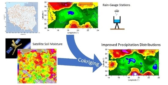
Improvement of Spatial Interpolation of Precipitation Distribution Using Cokriging Incorporating Rain-Gauge and Satellite (SMOS) Soil Moisture Data

Abstract

Precipitation data provide a crucial input for examining hydrological issues, including watershed management and mitigation of the effects of floods, drought, and landslides. However, they are collected frequently from the scarce and often insufficient network of ground-based rain-gauge stations to generate continuous precipitation maps. Recently, precipitation maps derived from satellite data have not been sufficiently linked to ground-based rain gauges and satellite-derived soil moisture to improve the assessment of precipitation distribution using spatial statistics. Kriging methods are used to enhance the estimation of the spatial distribution of precipitations. The aim of this study was to assess two geostatistical methods, ordinary kriging (OK) and ordinary cokriging (OCK), and one deterministic method (i.e., inverse distance weighting (IDW)) for improved spatial interpolation of quarterly and monthly precipitations in Poland and near-border areas of the neighbouring countries (~325,000 or 800,000 km²). Quarterly precipitation data collected during a 5-year period (2010–2014) from 113–116 rain-gauge stations located in the study area were used. Additionally, monthly precipitations in the years 2014–2017 from over 400 rain-gauge stations located in Poland were used. The spatiotemporal data on soil moisture (SM) from the Soil Moisture and Ocean Salinity (SMOS) global satellite (launched in 2009) were used as an auxiliary variable in addition to precipitation for the OCK method. The predictive performance of the spatial distribution of precipitations was the best for OCK for all quarters, as indicated by the coefficient of determination (R² = 0.944–0.992), and was less efficient (R² = 0.039–0.634) for the OK and IDW methods. As for monthly precipitation, the performance of OCK was considerably higher than that of IDW and OK, similarly as with quarterly precipitation. The performance of all interpolation methods was better for monthly than for quarterly precipitations. The study indicates that SMOS data can be a valuable source of auxiliary data in the cokriging and/or other multivariate methods for better estimation of the spatial distribution of precipitations in various regions of the world.

1. Introduction

Soil moisture–precipitation feedback provides a crucial input for numerous hydrological and agricultural issues, including watershed management [1], mitigation of the effects of floods and landslides [2], climate change [3,4,5,6,7], irrigation [8,9], waterborne diseases [10], field trafficability and soil tillage [11,12], and simulation of crop growth and productivity [13,14].

The spatial distribution of rainfall is frequently assessed using ground-based rain-gauge stations [15,16] since they provide the most precise and reliable measured data [17]. However, the network of the stations varies considerably and is often scarcely and not adequately distributed to obtain sufficiently dense point measurements for generating continuous high-quality rainfall maps in target areas [7,18,19]. Hence, to gain a suitable spatial distribution of precipitations based on point data, spatial interpolation methods should be used [18,20,21]. The recent literature review [22] may suggest a conclusion that, due to the particularly complex spatiotemporal variability and physical mechanism of rainfall, acquisition of rainfall data of high quality and resolution is still challenging.

Several spatial interpolation methods employing rain-gauge records have been developed (e.g., conventional trend surface analysis Thiessen polygons, deterministic methods such as inverse distance weighted (IDW) estimating values at unsampled points by the weighted average at surrounding points [23,24], and more complex geostatistical methods (e.g., kriging) that count the spatial dependence between rain gauges and the spatial arrangement around the forecasting place) [25,26,27,28]. The suitability of each interpolator depends on the environmental conditions, and hence, a comparative study aiming at the selection of the best method in the target area is recommended [4,15,29].

Precipitations frequently exhibit high spatial variability related to topographic and climate factors [30,31,32]. Therefore, to improve the estimation of the spatial distribution of rainfall, a multi-element survey using the geostatistical cokriging method can be appropriate [5,15,18,29]. The cokriging method allows the joint use of, for example, a sparsely distributed variable such as rain gauges and a densely sampled secondary variable that complements the former [26,27]. A recent study conducted by Adhikary et al. [15] revealed that elevation employed as a secondary variable in the cokriging method significantly enhanced the estimation of rainfall in Australian catchments with mountainous and complex terrain. In another recent study carried out by Pellicone et al. [29] in a mountainous region of Calabria (Italy), ordinary cokriging (OCK) and kriging with external drift (KED) interpolators using elevation and distance to the coastline as secondary variables improved the spatial rainfall distribution. However, in a relatively flat region in Belgium, the OCK and KED methods with elevation as a secondary variable did not enhance the estimation of spatial rainfall distribution [33]. In Swiss conditions, cokriging using temporal rain-gauge data as a secondary variable improved the estimations of the precipitations compared with radar estimates [34]. In another study [35], blending satellite and ground precipitation observations using a Bayesian kriging approach significantly improved the satellite-derived estimates. The above literature suggests that further developments that include new secondary variables are required to improve the prediction of the spatial distribution of rainfall.

A secondary variable that has not been used so far in the cokriging method is the soil moisture content available from satellite data of the Soil Moisture and Ocean Salinity (SMOS) mission [36,37]. Soil moisture (SM), in general, rises upon the incidence of rain events [38,39] and affects precipitation events on the other hand [40,41]. The SMOS mission launched in November 2009 [42] offers soil moisture observations for the topsoil (up to several centimetres’ depth) [43,44] using the interferometric radiometry method (1.4 GHz) from the orbit. SM data can be obtained every 1–3 days [45]. Validation has shown that SMOS SM data are well correlated with in situ soil moisture (R > 0.7) [46], exhibit reasonable root square mean error (RMSE) (≤0.04 m³ m⁻³) [43,46,47,48,49], and thus show good global performance [43,45]. Recent studies have demonstrated that assimilation of remotely sensed soil moisture has the potential to improve the quality of the near-real-time SMOS-based rainfall product [50,51] and to determine soil water resources [52].

It has been shown that the soil moisture–precipitation (SMP) feedback can be positive [53,54] or negative [55] depending on the environmental conditions. Several studies have demonstrated [40,53,56] that soil moisture information promotes rainfall generation, and the strength of this feedback is enhanced during warm seasons. In a study conducted by Vivoni et al. [40], the greater areal range of the storm maximum occurring in the high terrain of the Nacimiento Mountains was attributed to interaction between initial soil moisture and orographically induced rainfall. A negative SMP feedback was observed under a strong stability barrier at the top of the terrestrial boundary layer, which requires more sensible heat to induce appropriate turbulent mixing [55].

The main objective of this study was to examine whether satellite SMOS soil moisture data used along with rain-gauge records in the cokriging method are suitable for enhancing the estimation of the spatial distribution of quarterly (in the years 2010–2014) and monthly (in the years 2014–2017) precipitation over the area of Poland and near-border areas of neighbouring countries. The results of the cokriging method are compared with those of two methods (i.e., ordinary kriging and inverse distance weighting), which do not include satellite soil moisture data. Adequate evaluation of the spatial distribution of precipitation is important in a target area where rainfed agriculture is mostly practised and precipitation is the key uncertainty affecting water availability.

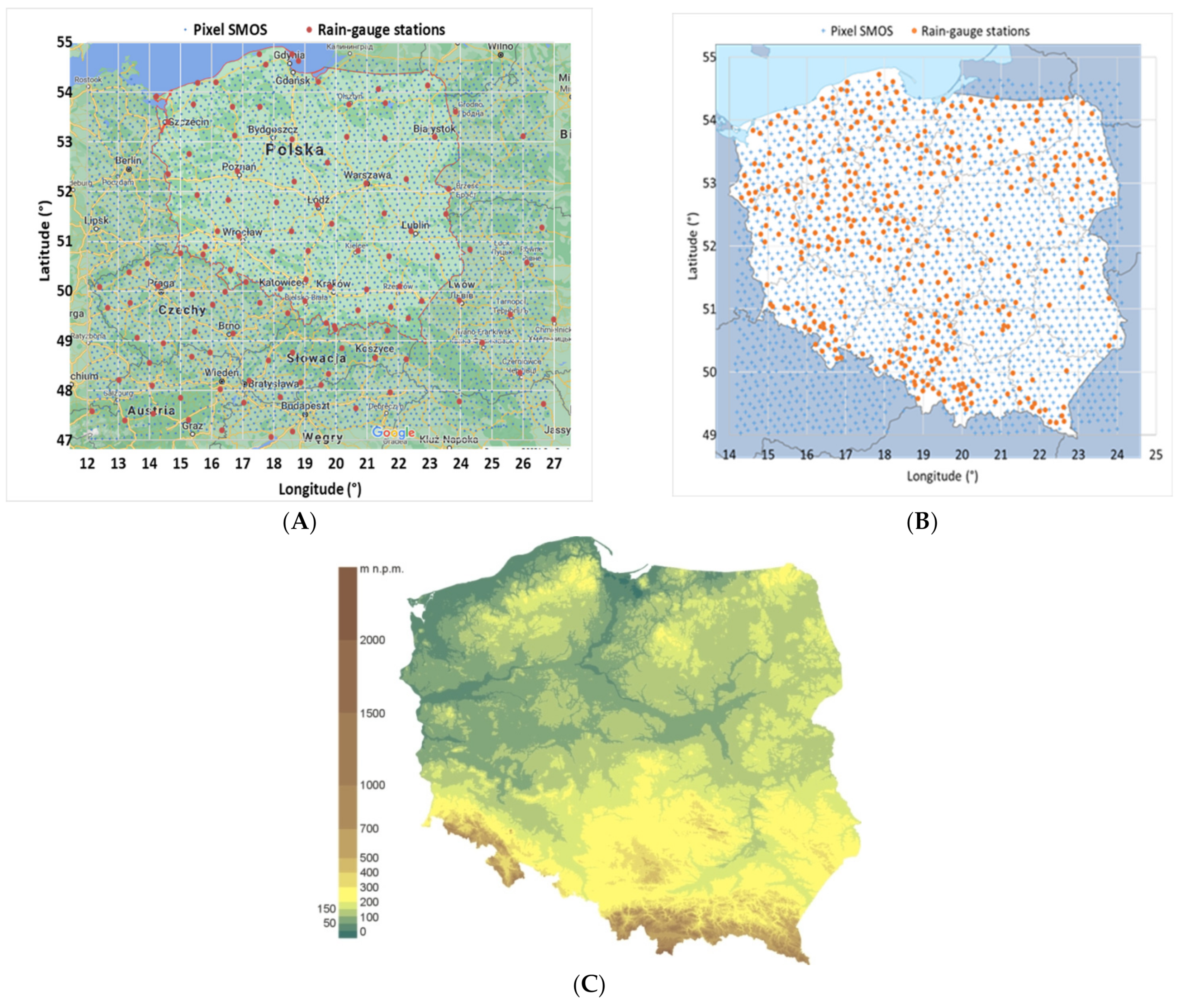
2. Study Area and Data Used

The study area included the whole territory of Poland and near-border areas of neighbouring countries (i.e., the Czech Republic, Slovakia, Ukraine, Belarus, Lithuania, and Russia), covering approximately 800,000 km². The study area is dominated by soils with texture of loamy sands and loams. In the case of the examined area of Poland, it was approximately 325,000 km². Quarterly precipitation data for a 5-year period (2010–2014) from 113–116 rain gauges retrieved from Tutiempo Network, S.L., Copyright 2018, located in a variety of networks were used (Figure 1A). Monthly precipitation data were obtained from over 400 ground meteorological stations of the Institute of Meteorology and Water Management—National Research Institute (IMGW) (Figure 1B). These free-access data are in ASCII format [57]. The original 1-day precipitation values were summed to monthly blocks in order to be consistent with the time scale of the SM from SMOS. It was assumed that a given weather station is representative of the entire SMOS pixel in which it is located. The rain-gauge stations were located at different altitudes varying from 1 to 1988 m a.s.l. The average altitude was 311 m with standard deviation as high as 320 m and, consequently, a coefficient of variation (average divided by standard deviation and multiplied by 100%) of 103%. The distribution of the altitudes exhibited a positive asymmetry and high slenderness. Skewness and kurtosis were 2.658 and 8.886, respectively. For this study, the SMOS L2 v. 650 datasets provided by the European Space Agency were examined. Based on the SMOS mission data processing algorithm, for each record assigned to a single DGG (Discrete Global Grid) node number, L2 retrieval has been carried out, under the condition that such pixel is not masked by no measurement value (−999 is assigned as an indicator of no measurements). The procedure for masking is defined by the series of quality flags defined in the mission Algorithm Theoretical Basis Document (ATBD) [58]. Additionally, variety of flags is applied to define the scene for which retrieval is conducted (including complex urban areas). The largest complications originate from external sources, such as radiofrequency interference (RFI) [58]. RFI contaminates the original signal, leading to exaggerated values of brightness temperature and, in consequence, unphysical values of SM. Thus, such pixels are masked by −999 (no measurement) value, before the L2 processing algorithm is applied. The datasets were downloaded from ftp://smos-ds-02.eo.esa.int/SMOS/L2SM/MIR_SMUDP2/. Next, further products were built from these data. The soil moisture contents in the topsoil (less than ~10 cm) were extracted from the SMOS satellite data for about 5000 (for Poland and neighbouring countries) and 2000 (for Poland) points on the Discrete Global Grid (15 km grid) using the Icosahedral Snyder Equal Area (ISEA) map 4H9 projection. SMOS soil moisture was averaged quarterly in 2010–2014 [59] and monthly in 2014–2017. For the purpose of geostatistical analysis, a regularization procedure was performed (i.e., it was assumed that each pixel is represented by one point located in its centre).

We validated the soil moisture data based on measured soil moisture at the stations in the Podlasie and Polesie regions using classical statistics, Bland–Altman plot, concordance correlation coefficient, and total deviation index. The validation results were satisfactory [49].

Basic statistics including mean, minimal, and maximal values for annual and monthly rainfall and soil moisture were calculated in 2010–2014 and 2014–2017 (Figure 2).

As can be seen in Figure 2A, the average annual precipitation totals were the greatest in 2010 (874 mm), and the smallest values were recorded in 2011 (599 mm) with an upward trend in the successive years, up to 704 mm (in 2014). The largest maximum annual fall was noted in 2010 (2157 mm in the mountains, 1989 m above sea level), whereas the smallest maximum was reported in 2011 (1433 mm at an altitude of 1327 m). The largest minimum annual fall was recorded in 2013 (462 mm, 323 m above sea level), and the lowest minimum was noted in 2011 (279 mm on 106 m above sea level). The variability of precipitation in 2010–2014 expressed by the coefficient of variation ranged from 29% to 35%.

The mean precipitation of monthly precipitations in the years 2014–2017 was 58.5 mm and generally lowest at the end of autumn to early spring (from 16 to 66 mm) and considerably greater in late spring to early autumn (from 71 to 131 mm) (Figure 2C). The coefficient of variability (CV) of the precipitations varied from about 25% to 85%. The variability was greater in autumn and winter than in spring and summer.

The mean soil moisture for the 5-year period (2010–2014) was 0.151 m³ m⁻³, with the highest and the lowest values in 2010 (0.171 m³ m⁻³) and in 2012 (0.128 m³ m⁻³), respectively (Figure 2B). The coefficients of variation were similar in all study years (26.6–33.3%). The minimum and maximum soil moisture values were close to zero and 0.5 m³ m⁻³. The skewness (0.20–0.57) and kurtosis (0.46–1.79) values indicate that soil moisture distribution was positively skewed and slightly narrow. The mean soil moisture in the individual quarters varied from 0.12 to 0.2 m³ m⁻³. The variability of soil moisture was, in general, highest in quarter I (to 40%) and lowest in quarter II (around 23%). The yearly standard deviations ranged from 0.04 to 0.051 m³ m⁻³. The standard variation was approximately 6.3% in quarter I and lower (up to ca. twofold) in the other quarters. The coefficient of variation was greater than 33% in each year and approximately 40% in quarter I of 2012 and 2013, with similar and lower variability in quarters II and III and increased variability in quarter IV. Histograms of soil moisture distributions indicate that the asymmetries were negative in quarter III and mostly positive in the other seasons (see Figure 3 in [59]). To obtain the normal distribution required in geostatistics, the variables with the highest asymmetry were transformed using the square root.

The mean soil moisture in the years 2014–2017 was 0.162 m³ m⁻³ with the highest and the lowest values of monthly soil moisture in January 2017 (0.085 m³ m⁻³) and in February 2017 (0.254 m³ m⁻³), respectively (Figure 2D). The coefficients of variation were generally similar in all study years (23.9%–48.0%) except January 2017 (97%). The minimum and maximum of monthly soil moisture values were respectively close to zero and 0.748 m³ m⁻³ (in wetlands). The values of skewness (−0.425 to 2.008) indicate that soil moisture distribution was slightly negatively and positively skewed, and those of kurtosis (−0.07 to 5.8) that it had a normal or narrow shape. Both the skewness and kurtosis values indicate that the monthly soil moisture distributions were close to the normal distribution.

3. Methodology

3.1. Semivariograms and Cross-Semivariograms

The analysis of the spatial dependence and distribution of precipitation (z₁) and soil moisture (z₂) was performed using geostatistical methods. The normality of precipitation was obtained after square root transformation. After that, the soil moisture distribution was close to normal and thereby met the required condition of a stationary or quasi-stationary process. The experimental semivariogram γ(h) and cross-semivariogram between precipitation (z₁) and soil moisture (z₂) − γ₁₂(h) for the distance h (°) were calculated from the following equations [60]:

$$\gamma \left(h\right)=\frac{1}{2N\left(h\right)}{\displaystyle \sum }_{i=1}^{N\left(h\right)}{\left[z_1\left(x_i\right)-z_1\left(x_i+h\right)\right]}^2$$

(1)

$${\gamma }_{12}\left(h\right)=\frac{1}{2N\left(h\right)}{\displaystyle \sum }_{i=1}^{N\left(h\right)}\left[z_1\left(x_i\right)-z_1\left(x_i+h\right)\right]·\left[z_2\left(x_i\right)-z_2\left(x_i+h\right)\right]$$

(2)

where N(h) is the number of pairs of points with values of [z₁(x_i), z₁(x_i+h)], [z₂(x_i), z₂(x_i+h)], distant by h, and x_i is the spatial coordinate. For semivariograms and cross-semivariograms determined empirically, the following three mathematical models were selected:

−

spherical model:

$$\gamma \left(h\right)=\left\{\begin{array}{ccc}{C}_0+C ·& \left[1.5\frac{\left|h\right|}{A_0}-0.5{\left(\frac{\left|h\right|}{A_0}\right)}^3\right]& \left|h\right|\le A_0\\ C_0+C & & h> A_0\end{array}\right.$$

(3)

−

exponential model:

$$\gamma \left(h\right)=C_0+C·\left[1-e^{-\frac{\left|h\right|}{A_0}}\right]\left|h\right|>0$$

(4)

−

Gaussian model:

$$\gamma \left(h\right)=C_0+C·\left[1-e^{-\frac{{\left|h\right|}^2}{A_0^2}}\right]\left|h\right|>0$$

(5)

where γ(h) is the semivariance for internal distance class h, h is the lag interval, C₀ is the nugget variance ≥0, C is the structural variance ≥C₀, A₀ is the range parameter, and C₀ + C is the sill. In the case of the spherical isotropic model, the effective range A = A₀. In the case of the exponential isotropic model, the effective range A = 3A₀, which is the distance at which the sill (C + C₀) is within 5% of the asymptote. In the case of the Gaussian model, the effective range A = 3^0.5A₀, which is the distance at which the sill (C + C₀) is within 5% of the asymptote. In the case of the anisotropic model, the effective range $A=\sqrt{A_1^2\left[{\mathit{cos}}^2\left(\theta -\phi \right)\right]+A_2^2\left[{\mathit{sin}}^2\left(\theta -\phi \right)\right]}$, where A₁ is the range parameter for the major axis (ϕ) and A₂ is the range parameter for the minor axis (ϕ + 90). In the case of the exponential anisotropic model, the range (or effective range) is 3A₁ for the major axis and 3A₂ for the minor axis, ϕ is the angle of maximum variation, and θ is the angle between pairs. In the case of the Gaussian anisotropic model, the range (or effective range) is 3^0.5A₁ for the major axis and 3^0.5A₂ for the minor axis, ϕ is the angle of maximum variation, and θ is the angle between pairs. To evaluate anisotropy, the azimuth direction A_z with the lowest semivariance values defined by smaller in the major direction (lower average semivariance) and largest in the minor (90°–offset) direction was used.

The obtained mathematical functions of semivariograms and cross-semivariograms were used for the spatial analysis of autocorrelation or for the visualization, through estimation, of the rainfall value under consideration in space with the kriging or cokriging methods. In places where no samples had been taken, the data were estimated using the IDW (inverse distance weighting), OK (ordinary kriging), and OCK (ordinary cokriging) methods. Experimental semivariograms were calculated based on the rainfall dataset and soil moisture for each quarter and month with consideration of the effect of distribution anisotropy of both quantities on the semivariogram parameters. The spherical, exponential, and Gaussian functions were fitted (selected) to the empirical semivariograms for each quarterly and monthly dataset of rainfalls and soil moisture. Then, models (functions) with the minimum residual sum of squares and the highest R² values were selected.

3.2. Interpolation Methods

A deterministic inverse distance weighting (IDW) and two geostatistical methods (i.e., ordinary kriging (OK) and ordinary cokriging (OCK)) were used to assess the spatial distribution of precipitations.

3.2.1. Inverse Distance Weighting

Inverse distance weighting (IDW) estimates values of precipitations at unsampled points by the weighted average of observed data at surrounding points [23,24]. Estimation of values in places where no samples had been taken was made with the inverse distance weighting method using the following equation [60]:

$$z_j^{*}\left(h\right)=\sum \frac{z_i}{{\left(h_{ij}+s\right)}^p}/\sum \frac{1}{{\left(h_{ij}+s\right)}^p}$$

(6)

where z_j*(h) is the estimated precipitation value at desired location j, z_i is the measured sample value at point i, h_j is the distance between z_j*(h) and z_i, s is the smoothing factor, and p is the weighting power.

3.2.2. Ordinary Kriging

Estimation of precipitation values in places where no samples had been taken was conducted with the kriging method [60]. The method yields the best nonbiased estimation of block values. This method also allowed for obtaining the minimum variance in the process of estimation. The estimator of kriging is a linear equation expressed by the following formula [60]:

$$z^{*}\left(x_o\right)={\displaystyle \sum }_{i=1}^N{\lambda }_{i}z\left(x_i\right)$$

(7)

where N is the number of measurements, z(x_i) is the value measured at point x_i, z*(x_o) is the estimated value at the point of estimation x_o, and λ_i is the weights. The weights are determined from a system of equations after inclusion of the condition of estimator nonbias and its effectiveness:

$$\left\{\begin{array}{lll}{\displaystyle \sum _{j=1}^N\lambda { }_j\gamma \left(x_i,x_j\right)}+\mu =\gamma \left(x_i,x_o\right)& & i=1\cdots N\\ {\displaystyle \sum _{i=1}^N\lambda { }_i}=1& & \end{array}\right.$$

(8)

3.2.3. Ordinary Cokriging (OCK)

Ordinary cokriging is a specific method for the analysis of random fields. It consists in the determination of covariance and reciprocal covariance as well as the cross-semivariogram function for specific parameters (i.e., precipitation (z₁) and soil moisture (z₂)). The main advantage of the method is the possibility of indirect reconstruction of the spatial variability of precipitation, the measurement of which is difficult and expensive, through field analysis of soil moisture, which is easier to determine with standard measuring equipment or available from satellite observations.

During the estimation of values at sites where no samples had been taken, x_o, can be made with the help of the estimation method known as the cokriging approach. The mathematical basis for cokriging is the theorem on the linear relationship of the unknown estimator z₂^*(x_o) expressed by the following formula [60]:

$$z_2^{*}\left(x_o\right)={\displaystyle \sum }_{i=1}^{N_1}{\lambda }_{1i}{z}_1\left(x_{1i}\right)+{\displaystyle \sum }_{j=1}^{N_2}{\lambda }_{2j}{z}_2\left(x_{2j}\right)$$

(9)

where λ_1i and λ_2j are weights associated with z₁ and z₂. N₁ and N₂ are the numbers of neighbours of z₁ and z₂ included in the estimation at point x_o. Cokriging weights are determined from a system of equations with the inclusion of the condition of estimator nonbias and its effectiveness:

$$\begin{array}{l}\left\{\begin{array}{l}{\displaystyle \sum _{i=1}^{N_1}\lambda { }_{1i}{C}_{11}\left(x_{1i},x_{1k}\right)}+{\displaystyle \sum _{j=1}^{N_2}\lambda { }_{2j}{C}_{12}\left(x_{1k},x_{2j}\right)}-{\mu }_1=C_{21}\left(x_o,x_{1k}\right)\hspace{1em}k=1, N_1\\ {\displaystyle \sum _{i=1}^{N_1}\lambda { }_{1i}{C}_{21}\left(x_{2l},x_{1i}\right)}+{\displaystyle \sum _{j=1}^{N_2}\lambda { }_{2j}{C}_{22}\left(x_{2j},x_{2l}\right)}-{\mu }_2=C_{22}\left(x_o,x_{2l}\right)\hspace{1em}l=1, N_2\\ {\displaystyle \sum _{i=1}^{N_1}\lambda { }_{1i}}=0\\ {\displaystyle \sum _{j=1}^{N_2}\lambda { }_{2j}}=1\end{array}\right.\\ \end{array}$$

(10)

where μ₁ and μ₂ are Lagrangian factors, and C₁₁, C₁₂, C₂₁, and C₂₂ represent covariance between the variables. The relationships between the semivariance γ(h) and the covariance C are expressed by the equation γ(h) = C(0) − C(h). In our study, the cokriging approach was used to enhance the estimation of spatial precipitation distribution using sparse data from rain-gauge stations and more densely sampled SMOS SM (as auxiliary variable) complementing the former.

Cross-validation analysis is used for evaluating effective parameters for IDW, kriging, and cokriging interpolations. In this analysis, each measured point in the area is individually removed, and its value is estimated based on neighbouring measurement points. Then the point is replaced, and the next point is removed and estimated, and so on. Finally, the estimations are compared with measured values in all points, and statistical parameters are determined [60].

4. Results

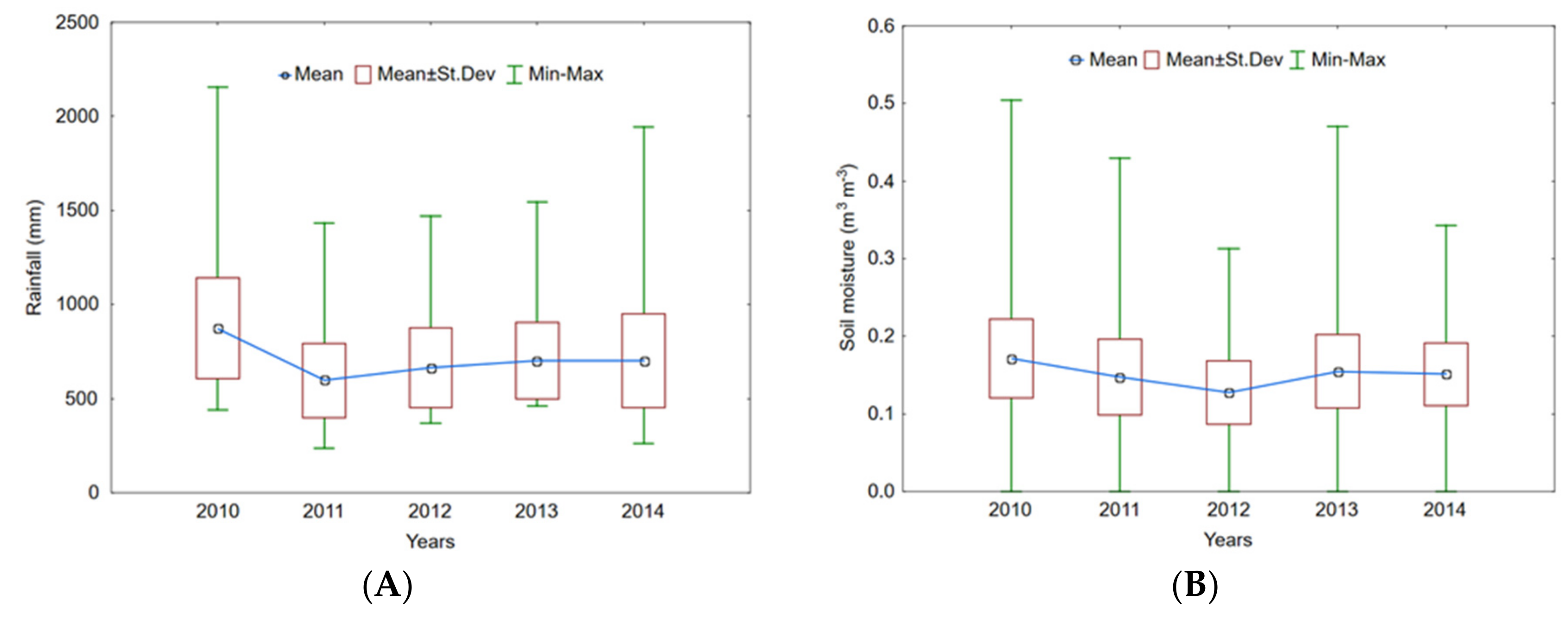
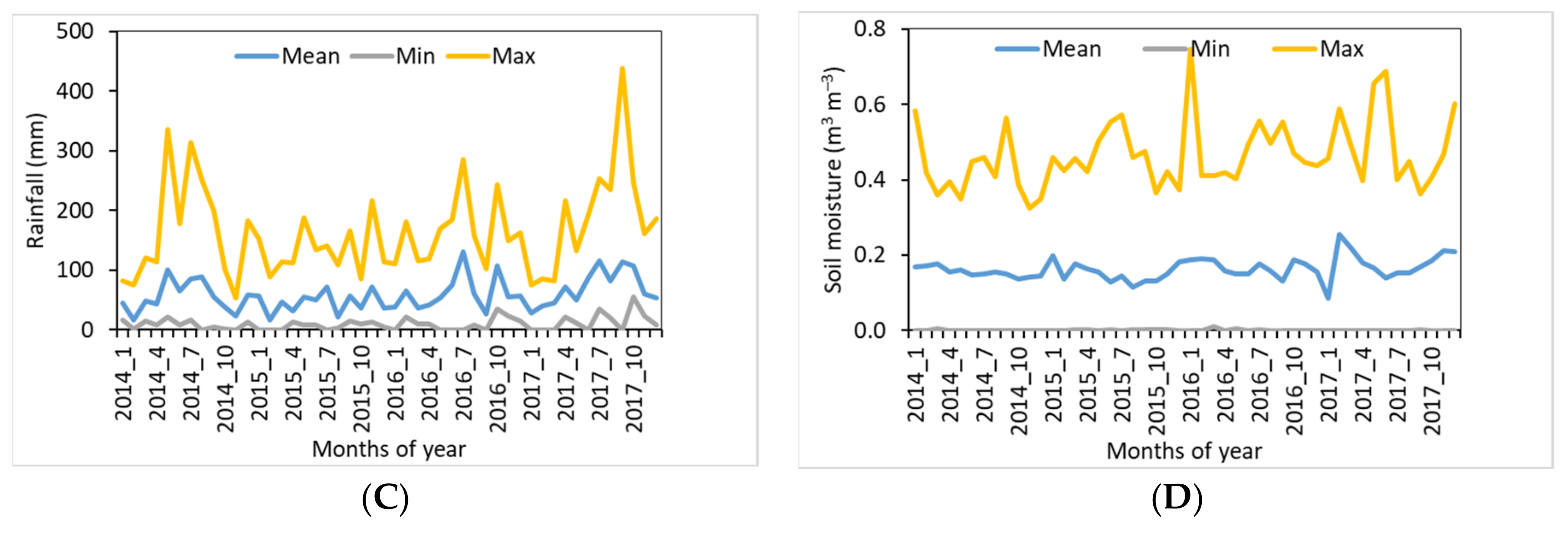
4.1. Statistics of Rain-Gauge Data

Table 1. Summary statistics for quarterly rainfall data of Poland and neighbouring countries.

Quarter of the Year	I 2010	II 2010	III 2010	IV 2010	I 2011	II 2011	III 2011	IV 2011	I 2012	II 2012	III 2012	IV 2012	I 2013	II 2013	III 2013	IV 2013	I 2014	II 2014	III 2014	IV 2014
n	115	115	116	116	116	116	113	116	115	116	116	116	114	114	114	114	114	116	116	110
Mean	104.0	277.1	344.0	148.3	80.6	163.3	261.1	91.7	113.8	185.5	219.4	145.5	141.0	265.5	190.2	106.5	93.8	207.9	275.5	114.1
SD	36.3	140.2	120.6	50.6	29.7	74.9	88.3	53.2	71.1	62.5	86.4	44.1	63.4	82.6	73.6	50.2	31.7	99.1	120.5	42.7
CV (%)	34.9	50.6	35.0	34.1	36.9	45.9	33.8	58.0	62.4	33.7	39.4	30.3	45.0	31.1	38.7	47.1	33.8	47.7	43.7	37.4
Min	29.2	26.7	157	49.3	30.2	46.7	94.8	23.1	11.2	69.6	53.6	69.6	48.5	129.3	37.6	27.2	31	23.8	75.5	55.4
Max	247.8	898.9	894.1	343.5	241.6	530.9	608.1	315.0	444.0	444.3	519.2	290.3	425.2	625.3	402.1	309.9	255.0	673.1	792.9	279.4
Skewness	1.302	1.523	1.998	0.847	1.947	2.045	0.900	1.900	2.312	1.166	1.034	1.071	1.535	1.163	1.042	1.477	1.165	2.081	1.360	1.523
Kurtosis	3.179	3.777	5.415	1.309	7.355	6.048	2.125	3.851	7.525	1.983	1.287	1.309	3.305	2.500	0.915	2.626	4.930	7.626	3.315	2.636
	Transformed rainfall data with a square root
Mean	10.1	16.2	18.3	12.0	8.8	12.5	15.9	9.3	10.3	13.4	14.5	11.9	11.6	16.1	13.6	10.1	9.6	14.1	16.2	10.5
SD	1.71	4.00	2.95	2.04	1.53	2.64	2.69	2.44	2.95	2.19	2.82	1.75	2.47	2.43	2.58	2.25	1.61	3.21	3.46	1.85
Skewness	0.524	0.526	1.327	0.282	0.985	1.178	0.239	1.239	1.008	0.679	0.455	0.653	0.888	0.633	0.465	0.853	0.218	0.621	0.575	1.020
Kurtosis	1.578	1.236	2.904	0.368	2.820	2.464	0.660	1.544	2.563	0.518	0.362	0.433	0.932	0.768	0.561	0.771	1.619	3.179	0.850	1.146

n—number of values, SD—standard deviation, CV—coefficient of variation, Min—minimum, Max—maximum.

presents the statistics of quarterly precipitations in 2010–2014. The mean precipitations were the lowest in quarters I and IV (80 and 150 mm) and considerably greater in quarters II and III (160 and 350 mm). The higher precipitations in the latter pair exhibited greater dispersion, as shown by the standard deviations. The coefficient of variability (CV) of the precipitations varied from about 30% to 62%. According to the literature [61], the CV values indicated moderate variability. The distribution of precipitations had a long and slender shape with positive asymmetries (values of 0.847–2.312) and large values of kurtosis (0.915–7.626). To meet the required condition of normality (or close to normality) in geostatistical analysis, the data were subjected to root square transformation, which led to lower asymmetries (0.218–1.327) and kurtosis (0.362–3.179).

The monthly precipitations in the years 2014–2017 varied largely from 0 to 438 mm, particularly during the summer (100–438 mm) (Figure 2). The distribution of precipitations had a slight asymmetry and slightly blurred shape with positive asymmetries (values of 0.0–1.5) and small values of kurtosis (−0.2 to 2.1) and was close to the normal distribution.

4.2. Correlation Analysis

As can be seen from

Table 2. Linear correlation coefficients between the quarterly and the monthly average rainfall and satellite soil moisture for Poland and neighbouring countries.

Correlation coefficients between the quarterly average rainfall and satellite soil moisture (P_SM) in the years 2010–2014. Bold, the correlation coefficients are significant with p < 0.05, n = 76.
P_SM_I 2010		P_SM_II 2010		P_SM_III 2010		P_SM_IV 2010		P_SM_I 2011		P_SM_II 2011		P_SM_III 2011		P_SM_IV 2011
−0.022		0.099		−0.062		0.237		0.234		0.238		0.289		0.335
P_SM_I 2012		P_SM_II 2012		P_SM_III 2012		P_SM_IV 2012		P_SM_I 2013		P_SM_II 2013		P_SM_III 2013		P_SM_IV 2013
0.191		0.184		0.187		0.195		0.038		0.307		0.2		0.196
P_SM_I 2014		P_SM_II 2014		P_SM_III 2014		P_SM_IV 2014
0.021		0.189		0.158		0.336
Correlation coefficients between the monthly average rainfall and satellite soil moisture (P_SM) in the years 2014–2017. Bold, the correlation coefficients are significant with p < 0.05, n = 391.
Years	P_SM _1		P_SM _2	P_SM _3	P_SM _4	P_SM _5	P_SM _6		P_SM _7	P_SM _8	P_SM _9	P_SM _10	P_SM _11		P_SM _12
2014	0.208		−0.028	−0.199	−0.186	−0.333	−0.090		−0.150	−0.063	−0.003	0.072	−0.206		0.131
2015	−0.087		−0.342	0.095	0.049	0.008	0.171		0.141	−0.118	0.309	−0.029	0.053		0.362
2016	−0.147		−0.260	−0.007	0.088	0.037	0.309		0.296	0.459	0.160	−0.155	0.454		0.316
2017	0.360		−0.012	0.200	0.054	0.025	0.210		0.255	0.376	0.203	0.429	0.271		0.441

P—precipitation (mm), SM—soil moisture (m³ m⁻³), 1–12 months.

, correlation coefficients between the quarterly average precipitations and the SMOS satellite soil moisture in the years 2010–2014 for Poland and neighbouring countries area were in 7 cases significantly positive (R from 0.234 to 0.336) and in 13 cases unexpectedly insignificant with positive or negative values. Correlation coefficients between the monthly average precipitations and the SMOS satellite soil moisture in the years 2014–2017 for Poland area were in 31 cases significantly negative (10) or positive (21) (R from −0.342 to −0.118 and from 0.131 to 0.459) and in the remaining 17 cases insignificant with positive or negative values.

It seems an obvious statement that soil moisture should increase when it rains and that there is no obstacle in reaching the soil surface. A positive and significant correlation between rainfall and soil moisture confirms the above statement for both quarterly and monthly rainfall data. The observed negative significant correlation between rainfall and soil moisture indicates that there are some factors in the studied areas that disturb this direction of soil moisture increase with increasing amounts of rainfall. Other factors changing this direction may be the soil texture and vegetation cover. We should also take into account the type of rainfall that occurs in a given area, whether it is frontal or convection rainfall limited to small areas. The type of rainfall will affect how quickly the water infiltrates into the soil, what part of the rainfall is captured by the vegetation, and how much water will evaporate from the soil and plant cover. Soil moisture in areas with coarse-textured soils can be less with more rainfall, and the inverse can be true in areas with fine-textured soils. Which of these factors and the relationships dominate in the study area and how they interact translate in turn into a correlation, whether it is significant, negative, positive, or insignificant.

4.3. Semivariogram and Cross-Variogram Models

The semivariograms and cross-semivariograms of paired precipitations with the SMOS satellite soil moisture for each year were calculated (

Table 3. Fitted semivariogram models for quarterly rainfall (P) and soil moisture (SM) data used in ordinary kriging interpolation method and cross-semivariogram models between rainfall and soil moisture (P_SM)—1° in the ordinary cokriging method corresponds to about 100 km.

	Semivariogram_P				C0/(C0 + C)			Semivariogram_SM			C0/(C0 + C)			Cross-semivariogram_P_SM
Year	Quarter	Model	C0	C0 + C		A (°)	Az (°)	Model	C0	C0 + C		A (°)	Az (°)	Model	C0	C0 + C	C0/(C0 + C)	A (°)	Az (°)
2010	I	Exp.	0.641	3.11	0.206	1.50	116	Exp.	0.00001	0.00335	0.003	1.00	105	Exp.	0.000	1.500	0.000	4.01	33
	II	Exp.	1.263	18.24	0.069	6.47	50	Exp.	0.00000	0.00176	0.001	1.62	58	Exp.	−0.002	−0.016	0.125	3.46	12
	III	Exp.	0.900	8.73	0.103	1.26	113	Exp.	0.00003	0.00168	0.017	1.54	66	Exp.	0.000	−0.016	0.000	8.11	12
	IV	Exp.	0.540	4.16	0.130	2.00	70	Exp.	0.00013	0.00205	0.063	1.88	116	Exp.	0.000	0.011	0.000	5.58	63
2011	I	Exp.	0.327	2.39	0.137	1.29	117	Exp.	0.00098	0.00327	0.298	2.73	97	Exp.	0.000	0.017	0.000	4.35	107
	II	Exp.	2.680	7.29	0.367	2.82	69	Exp.	0.00007	0.00114	0.060	1.73	124	Exp.	0.000	0.019	0.000	3.16	115
	III	Exp.	1.440	7.16	0.201	1.53	113	Exp.	0.00000	0.00131	0.002	1.70	41	Exp.	0.004	0.022	0.179	2.08	105
	IV	Exp.	0.100	5.48	0.018	1.49	120	Exp.	0.00013	0.00119	0.113	2.39	58	Gaus.	0.005	0.040	0.122	6.20	105
2012	I	Exp.	1.230	9.34	0.132	1.30	120	Exp.	0.00078	0.00371	0.209	2.03	58	Exp.	0.000	0.039	0.003	7.05	105
	II	Exp.	0.192	4.73	0.041	1.85	112	Exp.	0.00011	0.00108	0.106	1.63	154	Exp.	0.001	0.024	0.045	8.98	113
	III	Exp.	1.374	8.19	0.168	5.20	26	Exp.	0.00091	0.00142	0.642	2.73	0	Exp.	0.004	0.019	0.196	3.65	112
	IV	Exp.	0.312	3.17	0.098	1.42	106	Exp.	0.00092	0.00135	0.684	3.85	170	Exp.	0.000	−0.002	0.000	3.69	115
2013	I	Exp.	1.220	6.39	0.191	2.53	69	Exp.	0.00047	0.00290	0.163	1.81	131	Exp.	0.000	−0.025	0.000	2.30	45
	II	Exp.	1.690	6.75	0.250	6.12	76	Exp.	0.00000	0.00222	0.000	2.10	146	Exp.	0.000	0.008	0.013	2.67	122
	III	Exp.	2.534	7.32	0.346	3.28	105	Exp.	0.00057	0.00091	0.621	1.87	1	Exp.	0.008	0.019	0.403	5.04	112
	IV	Exp.	0.420	5.13	0.082	1.64	105	Exp.	0.00088	0.00154	0.570	4.08	172	Exp.	0.002	0.011	0.152	1.58	116
2014	I	Exp.	0.493	2.76	0.179	2.53	150	Exp.	0.00000	0.00127	0.001	1.49	86	Exp.	0.000	−0.006	0.000	5.88	112
	II	Exp.	1.420	10.70	0.133	1.64	108	Exp.	0.00000	0.00095	0.001	1.59	145	Exp.	0.000	0.012	0.000	2.91	114
	III	Exp.	2.119	12.39	0.171	5.73	108	Exp.	0.00078	0.00120	0.650	2.54	65	Exp.	0.000	0.016	0.000	2.34	117
	IV	Exp.	0.374	3.42	0.109	1.62	108	Exp.	0.00092	0.00184	0.498	1.73	145	Exp.	0.000	0.017	0.000	4.79	112
	Max		2.680	18.24	0.367	6.47	150		0.0010	0.0037	0.684	4.08	172.0		0.008	1.500	0.403	8.98	122
	Min		0.100	2.39	0.018	1.26	26		0.0000	0.0009	0.000	1.00	0.0		−0.002	−0.025	0.000	1.58	12
	1	Exp.	12.1	135.6	0.089	4.29	130	Exp.	0.00143	0.00340	0.421	3.46	101	Gaus.	0.000	0.115	0.001	2.40	103
	4	Exp.	101.9	308.3	0.331	4.96	93	Sph.	0.00097	0.00320	0.303	5.84	103	Gaus.	−0.001	−0.290	0.003	4.00	68
	7	Sph.	290.0	3422.0	0.085	4.66	93	Sph.	0.00119	0.00311	0.382	5.23	103	Gaus.	−0.001	−0.723	0.001	4.11	73
	10	Sph.	1.0	626.0	0.002	5.77	110	Exp.	0.00087	0.00278	0.313	4.47	81	Gaus.	−0.001	−0.067	0.015	3.87	73
2015	1	Sph.	29.0	434.0	0.067	2.28	86	Exp.	0.00160	0.00429	0.373	4.25	64	Gaus.	−0.001	−0.166	0.007	4.49	100
	4	Exp.	86.7	173.6	0.499	3.86	86	Exp.	0.00049	0.00252	0.194	2.49	62	Gaus.	−0.001	−0.111	0.009	4.48	87
	7	Exp.	231.5	551.9	0.419	2.67	71	Exp.	0.00103	0.00419	0.246	4.57	69	Gaus.	0.001	0.284	0.004	3.94	87
	10	Exp.	4.6	173.0	0.027	3.50	72	Exp.	0.00070	0.00273	0.256	4.77	58	Gaus.	0.000	−0.129	0.001	3.02	105
2016	1	Exp.	28.9	112.5	0.257	3.99	115	Sph.	0.00246	0.00863	0.285	5.46	95	Gaus.	0.000	−0.190	0.001	3.46	90
	4	Exp.	1.0	478.7	0.002	4.87	90	Exp.	0.00080	0.00224	0.357	5.16	66	Gaus.	−0.001	−0.181	0.006	3.38	110
	7	Exp.	145.0	2386.0	0.061	2.97	65	Exp.	0.00117	0.00383	0.305	4.66	74	Gaus.	0.000	0.359	0.000	3.61	120
	10	Exp.	320.0	1095.0	0.292	4.53	73	Exp.	0.00090	0.00345	0.261	4.98	78	Gaus.	−0.084	−1.240	0.068	4.28	120
2017	1	Exp.	0.0	210.0	0.000	3.73	77	Sph.	0.00127	0.00813	0.156	5.05	84	Gaus.	0.026	0.550	0.047	4.18	120
	4	Sph.	1.0	1603.0	0.001	4.35	83	Exp.	0.00104	0.00299	0.348	4.00	106	Gaus.	−0.001	−0.512	0.002	3.32	115
	7	Exp.	392.0	1592.0	0.246	4.17	60	Exp.	0.00090	0.00252	0.357	4.65	90	Gaus.	0.001	0.572	0.002	3.88	115
	10	Exp.	125.0	1239.0	0.101	3.75	90	Exp.	0.00075	0.00389	0.193	4.62	90	Gaus.	0.001	0.648	0.002	4.79	120
	Max		392.0	3422.0	0.499	5.77	130		0.0025	0.0086	0.421	5.84	106.0		0.026	0.648	0.068	4.79	120
	Min		0.0	112.5	0.000	2.28	60		0.0005	0.0022	0.156	2.49	58.0		−0.084	−1.240	0.000	2.40	68

Exp.—exponential model, Gaus.—Gaussian model, Sph.—the spherical model, C₀—nugget variance, C₀ + C—sill, A—effective range, A_z—anisotropy.

). The experimental values were best fitted (R² > 0.8) mostly to spherical, exponential, and Gaussian models. For quarterly precipitations and soil moisture, the best model to describe the spatial relationship was the exponential model. The ranges (A) of spatial dependence in semivariograms for quarterly precipitations were greater (from 1.26° for III 2010 to 6.47° for II 2010) with predominant values below 3 than for quarterly soil moisture contents (from 1.00° for I 2010 to 4.08° for IV 2013) with predominating values below 2° (Table 3). In the case of cross-semivariograms, the ranges of spatial dependence between rainfall and soil moisture appreciably increased, reaching a maximum of 8.98° with predominant values below 5°. Anisotropy (A_z) varied for precipitations from 50° to 120° with predominant values above 100°, for SMC from 0° to 172° with predominance below 120°, and for P_SM from 12° to 122° with predominance above 100°. The ratios C₀/(C₀ + C) were in most cases (50 out of 60) <0.25, indicating strong spatial dependence; in the other cases, it was moderate [62] (0.25–0.75). It is worth noting that the spatial dependences (nugget/sill) were more frequently stronger in OCK (0.00–0.179) (except one, 0.403) than OK (0.018–0.25).

In the case of semivariograms for monthly precipitations and soil moisture, the best models to describe the spatial relationship were the spherical and the exponential models. As for monthly precipitation in the years 2014–2017, the effective ranges (A) of spatial dependence in semivariograms varied from 2.28° for January 2015 to 5.77° for October 2015 with predominant values from 3.73° to 4.96°. The corresponding range for soil moisture contents was from 2.49 for April 2015 to 5.84 for April 2014 with predominant values >4°. In the case of cross-semivariograms, the best models to describe the spatial relationship were the Gaussian models. The effective ranges of spatial dependencies varied from 2.4° to 4.79° with predominant values above 3.61. The cross-semivariograms of monthly precipitations and soil moisture were negatively spatially dependent (10 times) and positively spatially dependent (6 times). Anisotropy (A_z) varied for precipitations and soil moisture from 58° to 130° with predominant values from 58° to 95° and P_SM from 100° to 120°. The ratios C₀/(C₀ + C) were in cases (16 out of 32) <0.25, indicating strong spatial dependence; in the other cases, it was moderate (0.25–0.75). It is worth noting that the spatial dependences (nugget/sill) were strong in OCK (0.00–0.068).

4.4. Comparison of the Interpolation Methods and Cross-Validation

The precipitation estimated with the use of the IDW, OK, and OCK methods was validated with the measured precipitation. The linear regression equation—y = ax + b, SE—standard error, R²—coefficient of determination, and SE Pre.—standard error prediction were calculated to compare the accuracy of each interpolator (

Table 4. Performance of inverse distance weighting (IDW), ordinary kriging (OK), and ordinary cokriging (OCK) for estimation of quarterly rainfall in Poland and neighbouring countries.

		IDW					Kriging (OK)					Cokriging (OCK)
Year	Quarter	a	SE	R2	b	SE Pre.	a	SE	R2	b	SE Pre.	a	SE	R2	b	SE Pre.
2010	I	0.552	0.230	0.048	47.9	35.4	0.610	0.248	0.051	42.4	36.4	1.441	0.029	0.957	−43.4	7.5
	II	1.062	0.082	0.599	−19.7	88.7	1.011	0.072	0.634	−1.3	87.8	1.066	0.009	0.992	−16.7	12.7
	III	0.983	0.194	0.183	2.3	108.9	1.030	0.216	0.166	−14.4	110.1	1.318	0.019	0.977	−108.8	18.3
	IV	0.996	0.159	0.256	6.6	43.6	1.000	0.165	0.244	7.2	44.0	1.229	0.019	0.974	−31.0	8.2
2011	I	0.651	0.302	0.039	29.6	29.3	0.734	0.339	0.040	23.7	29.3	1.428	0.019	0.980	−32.6	4.2
	II	1.206	0.151	0.358	−33.8	60.0	1.252	0.150	0.379	−39.4	59.0	1.386	0.032	0.944	−60.3	17.6
	III	1.393	0.209	0.285	−103.9	74.6	1.517	0.258	0.237	−136.8	77.1	1.371	0.020	0.978	−95.7	13.1
	IV	1.129	0.195	0.227	−6.6	46.7	1.140	0.217	0.195	−6.3	47.7	1.216	0.012	0.989	−17.5	5.6
2012	I	1.051	0.296	0.104	−0.5	67.9	1.100	0.325	0.095	−4.4	68.3	1.428	0.020	0.980	−43.4	10.2
	II	1.257	0.196	0.267	−44.2	53.8	1.206	0.210	0.226	−33.3	55.2	1.188	0.011	0.991	−33.2	6.0
	III	1.114	0.132	0.386	−22.4	67.7	0.983	0.115	0.391	7.7	67.4	1.162	0.019	0.970	−33.2	15.0
	IV	1.102	0.181	0.245	−11.1	38.3	1.119	0.200	0.200	−12.0	39.0	1.266	0.016	0.981	−36.6	6.1
2013	I	1.029	0.162	0.268	1.4	54.5	1.039	0.160	0.278	1.2	54.1	1.259	0.024	0.960	−33.3	12.7
	II	1.226	0.155	0.357	−61.4	66.2	1.119	0.133	0.387	−29.6	64.7	1.241	0.024	0.960	−62.3	16.6
	III	1.428	0.203	0.306	−73.7	61.4	1.388	0.192	0.317	−64.3	60.8	1.435	0.030	0.953	−76.8	16.0
	IV	1.102	0.180	0.251	−6.4	43.4	1.142	0.190	0.243	−9.0	43.7	1.240	0.015	0.985	−23.1	6.2
2014	I	0.755	0.165	0.157	23.5	29.1	0.796	0.161	0.179	19.9	28.7	1.260	0.024	0.960	−23.3	6.3
	II	1.062	0.184	0.227	−12.9	87.1	1.132	0.195	0.229	−26.6	87.0	1.290	0.018	0.977	−57.6	15.0
	III	1.099	0.092	0.557	−29.7	80.2	1.016	0.082	0.574	−3.8	78.6	1.129	0.020	0.965	−33.6	22.5
	IV	0.927	0.927	0.127	12.2	39.9	0.928	0.246	0.117	13.0	40.1	1.306	0.018	0.981	−32.4	5.9
	Max	1.428	0.927	0.599	47.9	108.9	1.517	0.339	0.634	42.4	110.1	1.441	0.032	0.992	−16.7	22.5
	Min	0.552	0.082	0.039	−103.9	29.1	0.610	0.072	0.040	−136.8	28.7	1.066	0.009	0.944	−108.8	4.2
	1	1.046	0.039	0.640	−2.1	6.7	0.930	0.037	0.612	3.2	7.1	1.077	0.011	0.964	−3.5	2.2
	4	1.021	0.048	0.538	−0.9	11.4	1.004	0.047	0.571	−0.2	10.9	1.162	0.023	0.864	−6.9	6.2
	7	1.013	0.036	0.665	−1.45	29.5	0.970	0.034	0.675	2.3	29	1.087	0.018	0.901	−7.4	16.0
	10	1.03	0.026	0.793	−1.08	9.6	0.947	0.024	0.797	1.8	9.5	1.026	0.005	0.992	−1.0	1.9
2015	1	1.058	0.042	0.636	−3	12.1	0.927	0.038	0.619	3.8	12.4	1.088	0.014	0.941	−4.9	4.9
	4	1.129	0.054	0.534	−3.6	9.0	1.086	0.049	0.559	−2.5	8.7	1.222	0.028	0.824	−6.8	5.5
	7	0.989	0.067	0.352	0.6	18.3	0.929	0.064	0.348	6.1	18.3	1.283	0.031	0.810	−20.5	9.9
	10	1.07	0.029	0.777	−2.5	6.2	1.013	0.024	0.815	−0.5	5.6	1.053	0.009	0.971	−1.9	2.3
2016	1	1.087	0.057	0.497	−2.9	7.3	1.004	0.050	0.525	0.0	7.1	1.213	0.019	0.915	−7.8	2.9
	4	1.018	0.025	0.807	−0.6	9.1	0.983	0.022	0.828	0.8	8.6	1.029	0.004	0.993	−1.2	1.7
	7	1.034	0.043	0.595	−5.7	29.3	0.939	0.039	0.589	7.5	29.5	1.103	0.009	0.974	−13.6	7.5
	10	1.05	0.036	0.678	−5.3	18.6	1.051	0.032	0.734	−5.4	16.9	1.146	0.016	0.924	−15.6	9.0
2017	1	1.052	0.035	0.759	−1.1	6.9	0.973	0.033	0.756	0.8	7.0	1.039	0.005	0.983	−1.1	1.1
	4	1.027	0.022	0.844	−2.5	13.8	0.982	0.020	0.865	1.1	12.8	1.018	0.004	0.995	−1.2	2.5
	7	1.019	0.038	0.644	−2.3	23.9	0.993	0.034	0.674	0.7	22.9	1.130	0.016	0.929	−15.2	10.7
	10	1.09	0.041	0.645	−9.1	19.5	0.996	0.035	0.672	0.7	18.7	1.101	0.010	0.967	−10.8	5.9
	Max	1.129	0.067	0.844	0.6	29.5	1.086	0.064	0.865	7.5	29.5	1.283	0.031	0.995	−1.0	16.0
	Min	0.989	0.022	0.352	−9.1	6.2	0.927	0.020	0.348	−5.4	5.6	1.018	0.004	0.810	−20.5	1.1

linear equation—y = ax + b, SE—standard error, R²—coefficient of determination, SE Pre.—standard error prediction.

). In the case of quarterly precipitation in the years 2010–2014, the ranges of regression coefficients (a), SE, SE Pre. (predicted), and R² for IDW and OK were 0.552–1.428, 0.082–0.927, 29.1–108.9, 0.039–0.599 and 0.610–1.517, 0.072–0.339, 28.7–110.1, 0.040–0.634, respectively (Table 4). These values indicate a slightly better accuracy of OK than IDW. In turn, OCK indicates that the directional coefficients (a) of regression equations are above 1, up to 1.44, with small SEs (<0.032) and SE Pre. (<23) and with high values of R² (>0.94). The R² values for IDW and OK, which are the lowest in quarter I in most years (in 3 of 5 years), correspond with the lowest precipitation, but are similar in all the quarters in the case of OCK (Table 4). The appreciably lower SE and SE Pre. values along with the higher R² for OCK than IDW and OK clearly indicate better performance of the former.

As for monthly precipitation in the years 2014–2017, the ranges of regression coefficients (a), SE, SE Pre. (predicted), and R² for IDW and OK were 0.989–1.129, 0.022–0.067, 6.2–29.5, 0.352–0.844 and 0.927–1.086, 0.020–0.064, 5.6–29.5, 0.348–0.865, respectively (Table 4). As for OCK, the values of regression coefficients (a) (1.018–1.283) were similar to those in IDW and OK, whereas those of SE (<0.031) and SE Pre. (<16) were lower, and R² (0.810–0.995) was in most cases considerably larger. The above data indicate better performance of OCK than IDW and OK, similarly as with quarterly precipitation.

Irrespective of the type of interpolation method used, the values of R² were larger, and those of SE and SE Pre. were lower for monthly than for quarterly precipitations (Table 4).

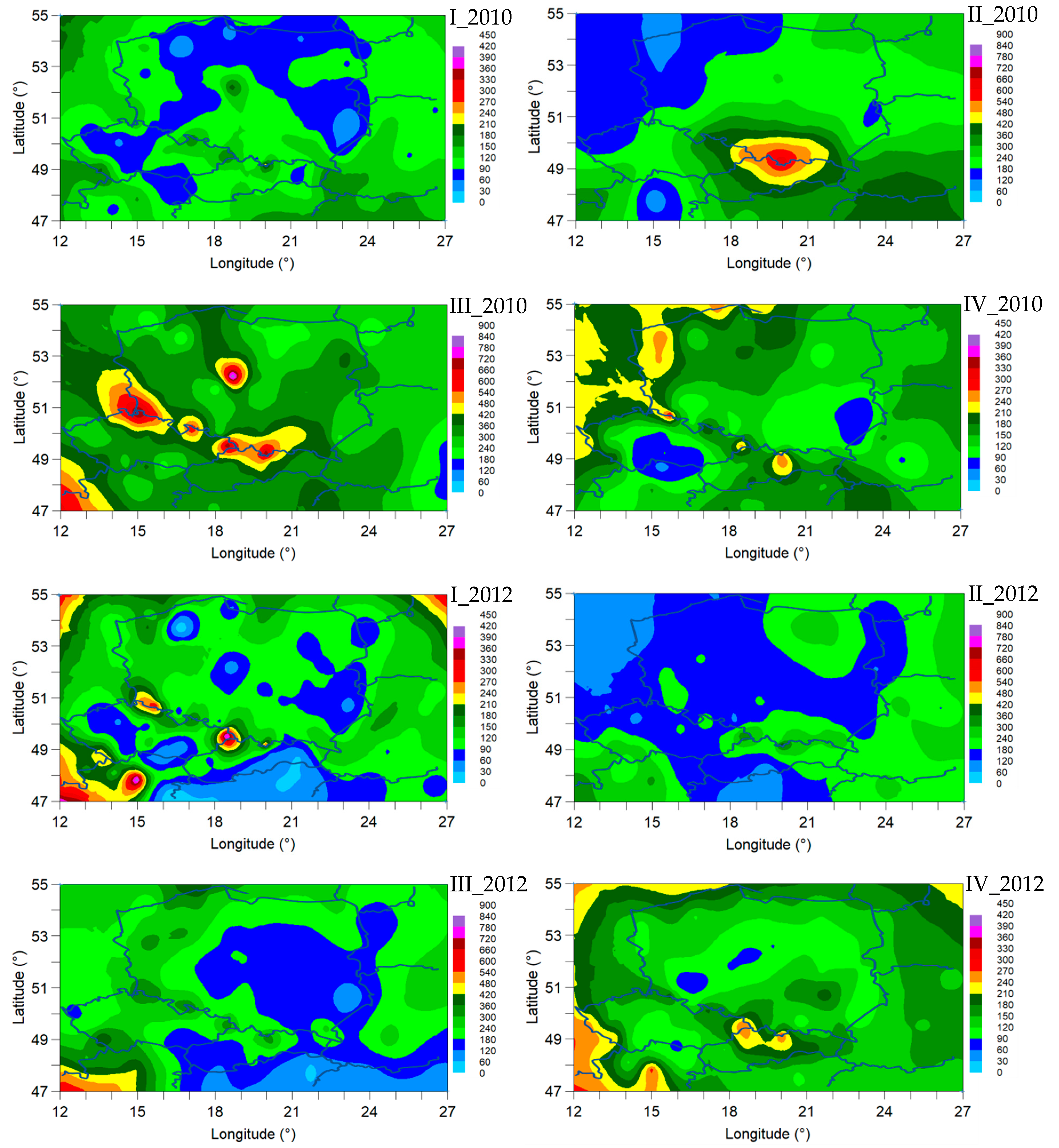
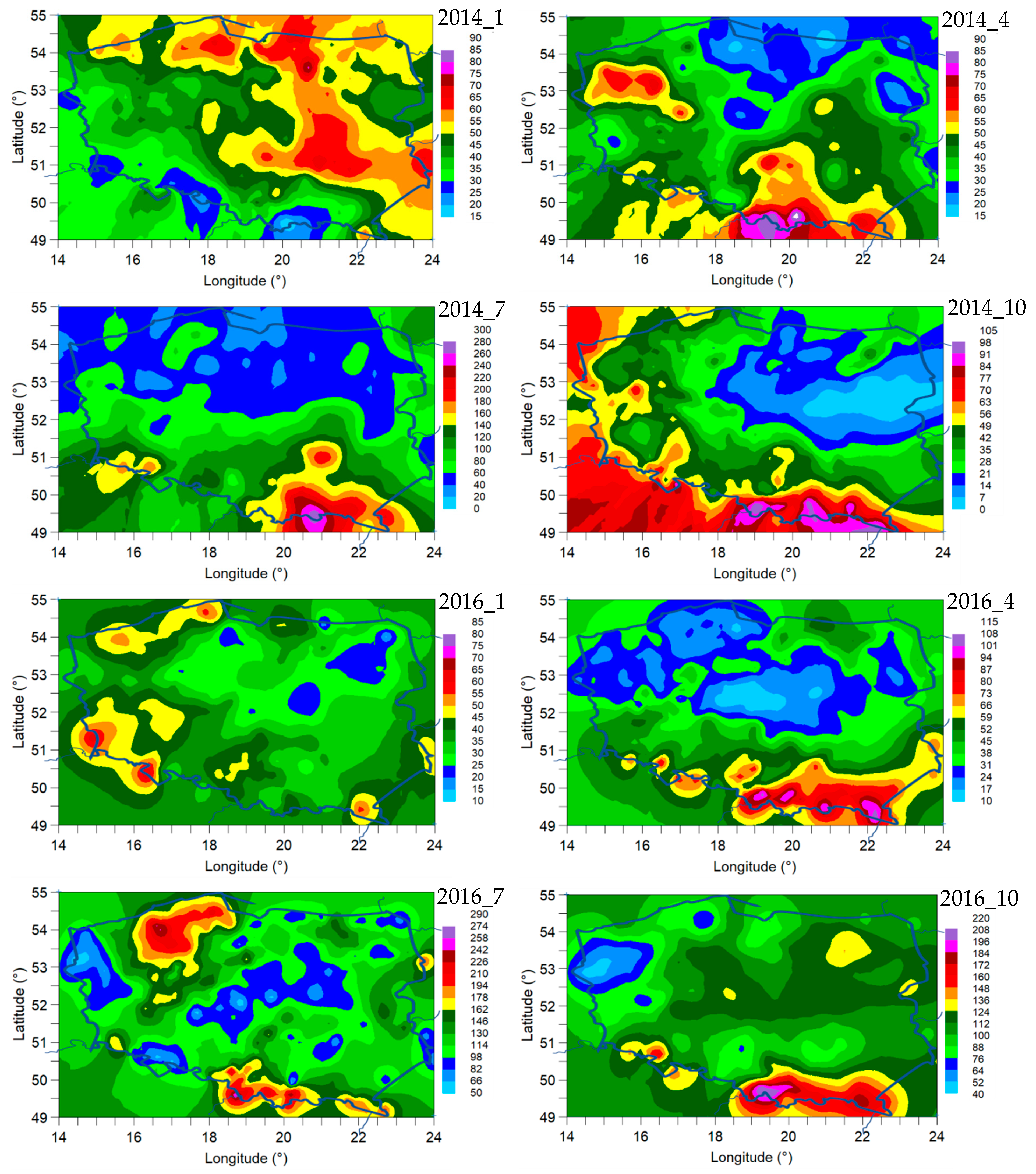
4.5. Maps of Precipitations

Figure 3 presents example spatial distributions of quarterly precipitations derived from the OCK approach, which gave the best estimation among the three tested methods. They include the years 2010 and 2012 among the 5 years analysed (2010–2014). The precipitations (in all years) were lower than 450 mm in quarters I and IV and below 900 mm in quarters II and III. The precipitations recorded in the mountainous measuring points were even two times greater than the estimated values (Figure 1) representing averages of both the high precipitation in the mountains and the lower precipitation in the neighbouring flat areas. In general, the variation in precipitation in the quarters is represented (characterized) by 3–4 and 10–13 colours, respectively, in the flat and less hilly areas with lower diversification of altitude and in the more mountainous areas with greater diversification (Figure 1C). Generally, this differentiation was mostly latitudinal and was reflected in the greater values of anisotropy (about 100°) (0° corresponds to anisotropy along the meridian) (Table 3). A targeted growth in anisotropy from quarters II to III from the northwest to the southeast was observed in all years, except 2013, when precipitations of snow were abundant in quarter II (especially in April). The increases in precipitation from quarters IV to I (in all years) were not so pronounced or targeted.

Figure 3 also presents the spatial distribution of monthly precipitations derived from the OCK method. Example distributions include the years 2014 and 2016 among the 4 years analysed (2014–2017). Variation of the monthly precipitation in Poland was generally smaller in winter and spring and much greater in summer and autumn (Figure 2 and Figure 3). As in the case of quarterly precipitations, the orientation of monthly precipitations was generally mostly latitudinal and was reflected in the greater values of anisotropy with predominant values above 90°. An anisotropy shift was observed from the northwest to the southeast to the west and the east from January to early October. Return to the previous orientation occurred in January of the following year, and the reorientation of anisotropy was repeated in the following years.

5. Discussion

Interpolation methods are increasingly being used and improved as tools to enhance estimation of the spatial precipitation distribution, as the availability of accurate observation data is limited. This study showed that the spatial prediction of quarterly precipitation data in Poland and near-border areas was more accurate when the ordinary cokriging (OCK) method was used with rain-gauge data (P) as the main variable and the satellite-derived soil moisture surface (SMOS SM) as an auxiliary variable (coefficients of determination R² = 0.944–0.992 between the measured and estimated precipitations), compared with both ordinary kriging (OK) (R² = 0.040–0.634) and inverse distance weighting (IDW) (R² = 0.039–0.599) using only the rain-gauge data. The greater suitability of the OCK method was supported by the smaller values of nugget and standard error prediction (SE Pre.) and the larger range of influence of the cross-semivariogram model than that of the direct (single) semivariogram for the above variables. As for monthly precipitation in the years 2014–2017, the performance of OCK (R² = 0.810–0.995) was considerably higher than that of IDW (R² = 0.352–0.844) and OK (R² = 0.348–0.865), similarly as with quarterly precipitation. The performance of all interpolation methods was better for monthly than for quarterly precipitations as shown by larger R² and lower SE and SE Pre. values.

Comparison of the present results and those from previous experiments indicates that the suitability of a given auxiliary variable depends on the topographic conditions of the studied areas. For example, in mountainous catchments of Australia at 25 to 1903 m a.s.l. [20] and the Calabria region in Italy [29] at <500 to 2266 m a.s.l., inclusion of elevation data as an auxiliary variable in the OCK method improved the prediction of the spatial distribution of orographically induced precipitations. However, this was not the case for the less hilly areas at 35 to 693 m a.s.l. in Belgium [33], where the OK and IDW methods performed better. Significant improvement of forecasting the spatial distribution of precipitations using OCK vs. OK and IDW observed in our study area with variable topography, including mountains, plateaus, plains, and valleys, may result from the fact that the topsoil (surface)-measured SMOS SM is sensitive to both small and large precipitation events in various topographic conditions. The suitability of satellite-derived SM data for improvement of prediction of spatial precipitation distribution based on rain-gauge data can be enhanced by their global availability [50,63,64]. The present analysis indicates that satellite-based remote sensing spatiotemporal soil moisture data can be a valuable source of an auxiliary variable for the cokriging and/or other multivariate (kriging) methods for better estimation of precipitations in various regions of the world. The performance of multivariate methods in the estimation of precipitation can be highlighted by recent attempts indicating that the spatial resolution of SMOS SM data can be increased by disaggregation of soil moisture from large to small pixels [65]. Additionally, it is possible to assess plant available water at a 0–50 cm depth based on the SMOS topsoil moisture using the Soil Water Index (SWI) and the exponential filter method as a proxy for the soil moisture in the root zone [47,63,66]. Furthermore, a combination of the previously developed approaches using satellite-derived soil moisture to improve satellite-based precipitation prediction [50,67] with the approach proposed in this study using satellite-derived soil moisture to improve rain-gauge-based precipitation prediction may have the considerable potential for upgrading precipitation prediction in future studies.

Improvement of precipitation predictability by the combination of ground rain-gauge data with satellite-derived soil moisture data can be particularly advantageous in transitional climate zones under the influence of, for example, dry and wet climates [68], where they may reduce the strength of the positive soil moisture–precipitation feedback or cause even reversed feedback [53,69]. This may result from, for example, dissimilar evapotranspiration [70] and/or surface albedo [71] as well as the related net radiation influencing the amount and intensity of precipitation. In the area of the present study, the relatively low strength of the soil moisture–precipitation feedback can be affected by the transitional climate zone between the oceanic climate dominating in the north and west and the continental climate in the south and east of the area [72]. Additionally, the predictability of precipitations in the study area can be influenced by the spatial variability of the soil cover including coarse-textured permeable soils [73] that exhibit lower water holding capacity and heat capacity [74,75,76] compared with fine-textured soils. This effect can be associated with different warming-up and evaporation rates of the soils. Furthermore, coarse-textured soils display greater sensitivity to different precipitation amounts than other soils [14]. In connection with this, potential water deficits in the study area result mostly from the lack of water in the proper place [77] observed especially in the central part of the study area with soil cover dominated by coarse-textured soil [73]. Therefore, the accurate prediction of spatial distribution of precipitation obtained with the OCK method is anticipated to be beneficial in spatial planning and managing hydrological issues and soil water resources at various time frames [32].

6. Summary and Conclusions

The spatial distribution of quarterly (years 2010–2014) and monthly precipitations (years 2014–2017) was estimated in Poland and near-border zones of neighbouring countries using inverse distance weighting interpolation (IDW) and ordinary kriging (OK) based on precipitation data from rain-gauge stations. The methods were compared for the first time with ordinary cokriging (OCK) incorporating rain-gauge data (main variable) and soil moisture data from SMOS satellite measurements (auxiliary variable). In comparison with the IDW and OK methods, OCK was identified as a much better interpolator of the spatial precipitation distribution, as shown by the predominantly larger coefficients of determination (0.944–0.992 vs. 0.039–0.634) for quarterly precipitations than those for monthly precipitations (0.810–0.995 vs. 0.348–0.865) and by geostatistical measures including the nugget, standard error prediction, and range values. Therefore, we recommend the OCK approach for the generation of the most accurate (continuous) map of precipitations. The performance of all interpolation methods was better for monthly than for quarterly precipitations. This study emphasizes that combining rain-gauge precipitation data and satellite-based SMOS soil moisture products has a positive impact on the performance of spatial prediction of precipitations. The SMOS data products cover areas of different elevations and precipitations and thus partially reflect the topography effects on soil moisture. Since they are available globally, satellite-derived SM data have the potential to be used as an auxiliary variable in multivariate methods to enhance the estimation of precipitations in different regions of the world.

References

1. Rivas-Tabares, D.; Tarquis, A.M.; Willaarts, B.; De Miguel, Á. An accurate evaluation of water availability in sub-arid Mediterranean watersheds through SWAT: Cega-Eresma-Adaja. Agric. Water Manag. 2019, 212, 211–225. [Google Scholar] [CrossRef] [Green Version]
2. Kalubowila, P.; Lokupitiya, E.; Halwatura, D.; Jayathissa, G. Threshold rainfall ranges for landslide occurrence in Matara district of Sri Lanka and findings on community emergency preparedness. Int. J. Disaster Risk Reduct. 2021, 52, 101944. [Google Scholar] [CrossRef]
3. Moral, F.J. Comparison of different geostatistical approaches to map climate variables: Application to precipitation. Int. J. Climatol. 2010, 30, 620–631. [Google Scholar] [CrossRef]
4. Delbari, M.; Afrasiab, P.; Jahani, S. Spatial interpolation of monthly and annual rainfall in northeast of Iran. Meteorol. Atmos. Phys. 2013, 122, 103–113. [Google Scholar] [CrossRef]
5. Ly, S.; Charles, C.; Degré, A. Different methods for spatial interpolation of rainfall data for operational hydrology and hydrological modeling at watershed scale: A review. Biotechnol. Agron. Soc. Environ. 2013, 17, 392–406. [Google Scholar]
6. Wu, H.; Adler, R.F.; Tian, Y.; Huffman, G.J.; Li, H.; Wang, J. Real-time global flood estimation using satellite-based precipitation and a coupled land surface and routing model. Water Resour. Res. 2014, 50, 2693–2717. [Google Scholar] [CrossRef] [Green Version]
7. Dao, D.A.; Kim, S.; Kim, T.-W.; Kim, D. Influence of rain gauge density and temporal resolution on the performance of conditional merging method. J. Korean Soc. Hazard Mitig. 2019, 19, 41–51. [Google Scholar] [CrossRef]
8. Fernández, J.E. Plant-based methods for irrigation scheduling of woody crops. Horticulturae 2017, 3, 35. [Google Scholar] [CrossRef] [Green Version]
9. Fernández, J.E.; Alcon, F.; Diaz-Espejo, A.; Hernandez-Santana, V.; Cuevas, M.V. Water use indicators and economic analysis for on-farm irrigation decision: A case study of a super high density olive tree orchard. Agric. Water Manag. 2020, 233, 106074. [Google Scholar] [CrossRef]
10. Rinaldo, A.; Bertuzzo, E.; Mari, L.; Righetto, L.; Blokesch, M.; Gatto, M.; Casagrandi, R.; Murray, M.; Vesenbeckh, S.M.; Rodriguez-Iturbe, I. Reassessment of the 2010–2011 Haiti cholera outbreak and rainfall-driven multiseason projections. Proc. Natl. Acad. Sci. USA 2012, 109, 6602–6607. [Google Scholar] [CrossRef] [Green Version]
11. Soane, B.D.; Ball, B.C.; Arvidsson, J.; Basch, G.; Moreno, F.; Roger-Estrade, J. No-till in northern, western and south-western Europe: A review of problems and opportunities for crop production and the environment. Soil Till. Res. 2012, 118, 66–87. [Google Scholar] [CrossRef] [Green Version]
12. Carranza, C.; Benninga, H.; van der Velde, R.; van der Ploeg, M. Monitoring agricultural field trafficability using Sentinel-1. Agric. Water Manag. 2019, 224, 105698. [Google Scholar] [CrossRef]
13. Morel, J.; Begue, A.; Todoroff, P.; Martine, J.; Lebourgeois, V.; Petit, M. Coupling a sugarcane crop model with the remotely sensed time series of fIPAR to optimise the yield estimation. Eur. J. Agron. 2014, 61, 60–68. [Google Scholar] [CrossRef]
14. Thaler, S.; Brocca, L.; Ciabatta, L.; Eitzinger, J.; Hahn, S.; Wagner, W. Effects of different spatial precipitation input data on crop model outputs under a Central European climate. Atmosphere 2018, 9, 290. [Google Scholar] [CrossRef] [Green Version]
15. Adhikary, S.K.; Muttil, N.; Yilmaz, A.G. Cokriging for enhanced spatial interpolation of rainfall in two Australian catchments. Hydrol. Process. 2017, 31, 2143–2161. [Google Scholar] [CrossRef] [Green Version]
16. Kerr, Y.H.; Al-Yaari, A.; Rodriguez-Fernandez, N.; Parrens, M.; Molero, B.; Leroux, D.; Bircher, S.; Mahmoodi, A.; Mialon, A.; Richaume, P.; et al. Overview of SMOS performance in terms of global soil moisture monitoring after six years in operation. Remote Sens. Environ. 2016, 180, 40–63. [Google Scholar] [CrossRef]
17. Lanza, L.G.; Vuerich, E. The WMO field intercomparison of rain intensity gauges. Atmos. Res. 2009, 94, 534–543. [Google Scholar] [CrossRef]
18. Goovaerts, P. Geostatistical approaches for incorporating elevation into the spatial interpolation of rainfall. J. Hydrol. 2000, 228, 113–129. [Google Scholar] [CrossRef]
19. Mirás Avalos, J.M.; Paz González, A.; Vidal Vázquez, E.; Sande Fouz, P. Mapping monthly rainfall data in Galicia (NW Spain) using inverse distances and geostatistical methods. Adv. Geosci. 2007, 10, 51–57. [Google Scholar] [CrossRef] [Green Version]
20. Adhikary, S.K.; Muttil, N.; Yilmaz, A.G. Ordinary kriging and genetic programming for spatial estimation of rainfall in the Middle Yarra River catchment, Australia. Hydrol. Res. 2016, 47, 1182–1197. [Google Scholar] [CrossRef]
21. Salleh, N.S.A.; Aziz, M.K.B.M.; Adzhar, N. Optimal design of a rain gauge network models: Review paper. J. Phys. Conf. Ser. 2019, 1366. [Google Scholar]
22. Hu, Q.; Li, Z.; Wang, L.; Huang, Y.; Wang, Y.; Li, L. Rainfall Spatial Estimations: A Review from Spatial Interpolation to Multi-Source Data Merging. Water 2019, 11, 579. [Google Scholar] [CrossRef] [Green Version]
23. Lu, G.Y.; Wong, D.W. An adaptive inverse-distance weighting spatial interpolation technique. Comput. Geosci. 2008, 34, 1044–1055. [Google Scholar] [CrossRef]
24. Chen, F.W.; Liu, C.W. Estimation of the spatial rainfall distribution using inverse distance weighting (IDW) in the middle of Taiwan. Paddy Water Environ. 2012, 10, 209–222. [Google Scholar] [CrossRef]
25. Isaaks, E.H.; Srivastava, R.M. Spatial continuity measures for probabilistic and deterministic geostatistics. Math. Geol. 1988, 20, 313–341. [Google Scholar] [CrossRef]
26. Zawadzki, J.; Cieszewski, C.J.; Zasada, M.; Lowe, R. Applying geostatistics for investigations of forest ecosystems using remote sensing imagery. Silva Fenn. 2005, 39, 599–617. [Google Scholar] [CrossRef] [Green Version]
27. Karahan, G.; Erşahin, S. Geostatistics in characterizing spatial variability of forest ecosystems. Eur. J. Sci. 2018, 6, 9–22. [Google Scholar]
28. Liu, S.; Li, Y.; Pauwels, V.R.N.; Walker, J.P. Impact of rain gauge quality control and interpolation on streamflow simulation: An application to the Warwick catchment, Australia. Front Earth Sci. 2018, 5, 114. [Google Scholar] [CrossRef] [Green Version]
29. Pellicone, G.; Caloiero, T.; Modica, G.; Guagliardi, I. Application of several spatial interpolation techniques to monthly rainfall data in the Calabria region (southern Italy). Int. J. Climatol. 2018, 9, 3651–3666. [Google Scholar] [CrossRef]
30. Chen, T.; Ren, L.; Yuan, F.; Yang, X.; Jiang, S.; Tang, T.; Liu, Y.; Zhao, C.; Zhang, L. Comparison of spatial interpolation schemes for rainfall data and application in hydrological modelling. Water 2017, 9, 342. [Google Scholar] [CrossRef] [Green Version]
31. Sadeghi, S.H.; Nouri, H.; Faramarzi, M. Assessing the spatial distribution of rainfall and the effect of altitude in Iran (Hamadan Province). Air Soil Water Res. 2017, 10, 1–7. [Google Scholar] [CrossRef]
32. Berndt, C.; Haberlandt, U. Spatial interpolation of climate variables in Northern Germany—Influence of temporal resolution and network density. J. Hydrol. Reg. Stud. 2018, 15, 184–202. [Google Scholar] [CrossRef]
33. Ly, S.; Charles, C.; Degré, A. Geostatistical interpolation of daily rainfall at catchment scale: The use of several variogram models in the Ourthe and Ambleve catchments, Belgium. Hydrol. Earth Syst. Sci. 2011, 15, 2259–2274. [Google Scholar] [CrossRef] [Green Version]
34. Sideris, I.V.; Gabella, M.; Erdin, R.; Germann, U. Real-time radar-rain-gauge merging using spatio-temporal co-kriging with external drift in the alpine terrain of Switzerland. Q. J. R. Meteor. Soc. 2014, 140, 1097–1111. [Google Scholar] [CrossRef]
35. Verdin, A.; Rajagopalan, B.; Kleiber, W.; Funk, C. A Bayesian kriging approach for blending satellite and ground precipitation observations. Water Resour. Res. 2015, 51. [Google Scholar] [CrossRef]
36. Kerr, Y.H. Soil moisture from space: Where are we? Hydrogeol. J. 2007, 15, 117–120. [Google Scholar] [CrossRef]
37. Wagner, W.; Blöschl, G.; Pampaloni, P.; Calvet, J.C.; Bizzarri, B.; Wigneron, J.P.; Kerr, Y. Operational readiness of microwave remote sensing of soil moisture for hydrologic applications. Hydrol. Res. 2007, 38, 1–20. [Google Scholar] [CrossRef]
38. McColl, K.A.; Wang, W.; Peng, B.; Akbar, R.; Short Gianotti, D.J.; Lu, H.; Pan, M.; Entekhabi, D. Global characterization of surface soil moisture dry downs. Geophys. Res. Lett. 2017, 44, 3682–3690. [Google Scholar] [CrossRef]
39. McColl, K.A.; Alemohammad, S.H.; Akbar, R.; Konings, A.G.; Yueh, S.; Entekhabi, D. The global distribution and dynamics of surface soil moisture. Nat. Geosci. 2017, 10, 100–104. [Google Scholar] [CrossRef]
40. Vivoni, E.R.; Tai, K.; Gochis, D.J. Effects of initial soil moisture on rainfall generation and subsequent hydrologic response during the North American monsoon. J. Hydrometeor. 2009, 10, 644–663. [Google Scholar] [CrossRef] [Green Version]
41. Kim, H.; Lakshmi, V. Global dynamics of stored precipitation water in the topsoil layer from satellite and reanalysis data. Water Resour. Res. 2019, 55, 3328–3346. [Google Scholar] [CrossRef]
42. Kerr, Y.H.; Waldteufel, P.; Wigneron, J.; Delwart, S.; Cabot, F.; Boutin, J.; Escorihuela, M.; Font, J.; Reul, N.; Gruhier, C.; et al. The SMOS mission: New tool for monitoring key elements of the Global Water Cycle. Proc. IEEE 2010, 98, 666–687. [Google Scholar] [CrossRef] [Green Version]
43. Al-Yaari, A.; Wigneron, J.P.; Ducharne, A.; Kerr, Y.H.; Wagner, W.; De Lannoy, G.; Reichle, R.; Al Bitar, A.; Dorigo, W.; Richaume, P.; et al. Global-scale comparison of passive (SMOS) and active (ASCAT) satellite based microwave soil moisture retrievals with soil moisture simulations (MERRA-Land). Remote Sens. Environ. 2014, 152, 614–626. [Google Scholar] [CrossRef] [Green Version]
44. Escorihuela, M.J.; Chanzy, A.; Wigneron, J.P.; Kerr, Y.H. Effective soil moisture sampling depth of L-band radiometry: A case study. Remote Sens. Environ. 2010, 114, 995–1001. [Google Scholar] [CrossRef] [Green Version]
45. Kerr, Y.H.; Waldteufel, P.; Richaume, P.; Wigneron, J.P.; Ferrazzoli, P.; Mahmoodi, A.; Bitar, A.A.; Cabot, F.; Gruhier, C.; Juglea, S.E.; et al. The SMOS soil moisture retrieval algorithm. IEEE Trans. Geosci. Remote Sens. 2012, 50, 1384–1403. [Google Scholar] [CrossRef]
46. Escorihuela, M.J.; Merlin, O.; Stefan, V.; Moyano, G.; Eweys, O.A.; Zribi, M.; Kamara, S.; Benahi, A.S.; Ebbe, M.A.B.; Chihrane, J.; et al. SMOS based high resolution soil moisture estimates for desert locust preventive management. Remote Sens. Appl. Soc. Environ. 2018, 11, 140–150. [Google Scholar]
47. González-Zamora, Á.; Sánchez, N.; Martínez-Fernández, J.; Wagner, W. Root-zone plant available water estimation using the SMOS-Derived Soil Water Index. Adv. Water Resour. 2016, 96, 339–353. [Google Scholar] [CrossRef]
48. Deng, K.A.K.; Lamine, S.; Pavlides, A.; Petropoulos, G.P.; Bao, Y.; Srivastava, P.K.; Guan, Y. Large scale operational soil moisture mapping from passive MW radiometry: SMOS product evaluation in Europe & USA. Int. J. Appl. Earth Obs. Geoinf. 2019, 80, 206–217. [Google Scholar] [CrossRef]
49. Usowicz, B.; Marczewski, W.; Usowicz, J.B.; Łukowski, M.I.; Lipiec, J. Comparison of surface soil moisture from SMOS satellite and ground measurements. Int. Agrophys. 2014, 28, 359–369. [Google Scholar] [CrossRef] [Green Version]
50. Brocca, L.; Pellarin, T.; Crow, W.D.; Ciabatta, L.; Massari, C.; Ryu, D.; Su, C.H.; Rüdiger, C.; Kerr, Y. Rainfall estimation by inverting SMOS soil moisture estimates: A comparison of different methods over Australia. J. Geophys. Res. Atmos. 2016, 121, 12062–12079. [Google Scholar] [CrossRef]
51. Brocca, L.; Filippucci, P.; Hahn, S.; Ciabatta, L.; Massari, C.; Camici, S.; Schüller, L.; Bojkov, B.; Wagner, W. SM2RAIN–ASCAT (2007–2018): Global daily satellite rainfall data from ASCAT soil moisture observations. Earth Syst. Sci. Data 2019, 11, 1583–1601. [Google Scholar] [CrossRef] [Green Version]
52. Usowicz, B.; Lukowski, M.; Lipiec, J. The SMOS-Derived Soil Water EXtent and equivalent layer thickness facilitate determination of soil water resources. Sci. Rep. 2020, 10, 18330. [Google Scholar] [CrossRef]
53. Xu, J.J.; Shuttleworth, W.J.; Gao, X.; Sorooshian, S.; Small, E.E. Soil moisture-precipitation feedback on the North American monsoon system in the MM5-OSU model. Quart. J. R. Meteor. Soc. 2004, 130, 2873–2890. [Google Scholar] [CrossRef]
54. Moon, H.; Guillod, B.P.; Gudmundsson, L.; Seneviratne, S.I. Soil moisture effects on afternoon precipitation occurrence in current climate models. Geophys. Res. Lett. 2019, 46, 1861–1869. [Google Scholar] [CrossRef] [PubMed] [Green Version]
55. Hohenegger, C.; Brockhaus, P.; Bretherton, C.S.; Schär, C. The soil moisture–precipitation feedback in simulations with explicit and parameterized convection. J. Climatol. 2009, 22, 5003–5020. [Google Scholar] [CrossRef]
56. Hong, S.-Y.; Pan, H.-L. Impact of soil moisture anomalies on seasonal, summertime circulation over North America in a regional climate model. J. Geophys. Res. 2000, 105, 29625–29634. [Google Scholar] [CrossRef]
57. Public Data Base IMGW-PIB. Available online: https://danepubliczne.imgw.pl/ (accessed on 15 October 2020).
58. Kerr, Y.H.; Waldteufel, P.; Richaume, P.; Wigneron, J.P.; Ferrazzoli, P.; Gurney, R. SMOS Level 2 Processor for Soil Moisture—Algorithm Theoretical Based Document (ATBD); Technic Report SO-TN-ESL-SM-GS-0001; Array Systems Computing Inc.: Toronto, ON, Canada, 2011; Chapter 3.4.4.1; pp. 1–123. [Google Scholar]
59. Usowicz, B.; Lipiec, J.; Łukowski, M. Evaluation of soil moisture variability in Poland from SMOS satellite observations. Remote Sens. 2019, 11, 1280. [Google Scholar] [CrossRef] [Green Version]
60. Robertson, G.P. GS+: Geostatistics for the Environmental Sciences; Gamma Design Software: Plainwell, MI, USA, 2008. [Google Scholar]
61. Nielsen, D.R.; Bouma, J. Soil spatial variability. In Proceedings of the a Workshop of the ISSS and the SSSA, Las Vegas, NV, USA, 30 November–1 December 1984; p. 243. [Google Scholar]
62. Cambardella, C.A.; Moorman, T.B.; Parkin, T.B.; Karlen, D.L.; Novak, J.M.; Turco, R.F.; Konopka, A.E. Field-scale variability of soil properties in Central Iowa soils. Soil Sci. Soc. Am. J. 1994, 58, 1501–1511. [Google Scholar] [CrossRef]
63. Kwon, M.; Han, D. Assessment of remotely sensed soil moisture products and their quality improvement: A case study in South Korea. J. Hydro Environ. Res. 2019, 24, 14–27. [Google Scholar] [CrossRef]
64. Das, N.N.; Entekhabi, D.; Dunbar, R.S.; Njoku, E.G.; Yueh, S.H. Uncertainty estimates in the SMAP combined active–passive downscaled brightness temperature. IEEE Trans. Geosci. Remote Sens. 2016, 54, 640–650. [Google Scholar] [CrossRef]
65. Khodayar, S.; Coll, A.; Lopez-Baeza, E. An improved perspective in the spatial representation of soil moisture: Potential added value of SMOS disaggregated 1 km resolution “all weather” product. Hydrol. Earth Syst. Sci. 2019, 23, 255–275. [Google Scholar] [CrossRef] [Green Version]
66. Kędzior, M.; Zawadzki, J. SMOS Data as a source of the agricultural drought information: Case study of the Vistula Catchment, Poland. Geoderma 2017, 306, 167–182. [Google Scholar] [CrossRef]
67. Wanders, N.; Pan, M.; Wood, E.F. Correction of real-time satellite precipitation with multi-sensor satellite observations of land surface variables. Remote Sens. Environ. 2015, 160, 206–221. [Google Scholar] [CrossRef]
68. Koster, R.D.; Dirmeyer, P.A.; Guo, Z.; Bonan, G.; Chan, E.; Cox, P.; Gordon, C.T.; Kanae, S.; Kowalczyk, E.; Lawrence, D.; et al. Regions of strong coupling between soil moisture and precipitation. Science 2004, 305, 1138–1140. [Google Scholar] [CrossRef] [Green Version]
69. Ek, M.B.; Holstag, A.A.M. Influence of soil moisture on boundary layer cloud development. J. Hydrometeorol. 2004, 5, 86–99. [Google Scholar] [CrossRef]
70. Zheng, X.Y.; Eltahir, E.A.B. A soil moisture–rainfall feedback mechanism. 2. Numerical experiments. Water Resour. Res. 1998, 34, 777–785. [Google Scholar] [CrossRef] [Green Version]
71. Vivoni, E.R.; Moreno, H.A.; Mascaro, G.; Rodriguez, J.C.; Watts, C.J.; Garatuza-Payan, J.; Scott, R.L. Observed relation between evapotranspiration and soil moisture in the North American monsoon region. Geophys. Res. Lett. 2008, 35, L22403. [Google Scholar] [CrossRef] [Green Version]
72. Kundzewicz, Z.W.; Førland, E.J.; Piniewski, M. Challenges for developing national climate services—Poland and Norway. Climate Serv. 2017, 8, 17–25. [Google Scholar] [CrossRef]
73. Usowicz, Ł.B.; Usowicz, B. Spatial variability of soil particle size distribution in Poland. In Proceedings of the 17th World Congress of Soil Science, Bangkok, Thailand, 14–21 August 2002; pp. 1–10. [Google Scholar]
74. Walczak, R.; Ostrowski, J.; Witkowska-Walczak, B.; Slawinski, C. Hydrophysical characteristics of Polish arable mineral soils (in Polish). Acta Agrophys. 2002, 79, 1–64. [Google Scholar]
75. Bieganowski, A.; Witkowska-Walczak, B.; Gliński, J.; Sokołowska, Z.; Sławiński, C.; Brzezińska, M.; Włodarczyk, T. Database of Polish arable mineral soils: A review. Int. Agrophys. 2013, 27, 335–350. [Google Scholar] [CrossRef] [Green Version]
76. Usowicz, B.; Marczewski, W.; Lipiec, J.; Usowicz, J.B.; Sokołowska, Z.; Dąbkowska-Naskręt, H.; Hajnos, M.; Łukowski, M.I. Water in the Soil—Ground and Satellite Measurements in Studies on Climate Change; Foundation for the Development of Agrophysical Sciences, Committee for Agrophysics PAS, Monograph: Lublin, Poland, 2009. (In Polish) [Google Scholar]
77. Orlińska-Woźniak, P.; Wilk, P.; Gębala, J. Water availability in reference to water needs in Poland. Meteor. Hydrol. Water Manag. 2013, 1, 45–50. [Google Scholar] [CrossRef] [Green Version]
Figure 1. Spatial distribution of rain-gauge stations in Poland and neighbouring countries and SMOS pixel (A). Map was created using Google Earth (v. 7.3.2.5776). Google, proprietary software, https://www.google.com/earth/. The background maps from Google Maps (https://www.google.com/maps/@51.1367607,20.6545385,5.5z), accessed 12 April 2017, and https://pl.wikipedia.org/wiki/Plik:Poland_location_map_white.svg (B). Elevation map of Poland, n.p.m.—above sea level (C), https://pl.wikipedia.org/wiki/Mapa_hipsometryczna#/media/Plik:Poland-hipsometric_map.jpg. The background maps were modified using Microsoft Office PowerPoint 2019.
Remotesensing 13 01039 g001
Figure 2. Mean, minimal (Min), and maximal (Max) values for annual rainfall (A) and soil moisture data (B) with standard deviations in Poland and neighbouring countries for the study period 2010–2014 and for monthly rainfall (C) and soil moisture data (D) in Poland for the study period 2014–2017.
Remotesensing 13 01039 g002aRemotesensing 13 01039 g002b
Figure 3. Spatial distribution of monthly rainfall (2D maps) in Poland estimated by the ordinary cokriging interpolation method for selected months in the years 2014 and 2016 (1° = approximately 100 km). Maps were created using Gamma Design Software GS+10 [60].
Remotesensing 13 01039 g003aRemotesensing 13 01039 g003b