Abstract
Information about forest cover and its characteristics are essential in national and international forest inventories, monitoring programs, and reporting activities. Two of the most common forest variables needed to support sustainable forest management practices are forest cover area and growing stock volume (GSV m3 ha−1). Nowadays, national forest inventories (NFI) are complemented by wall-to-wall maps of forest variables which rely on models and auxiliary data. The spatially explicit prediction of GSV is useful for small-scale estimation by aggregating individual pixel predictions in a model-assisted framework. Spatial knowledge of the area of forest land is an essential prerequisite. This information is contained in a forest mask (FM). The number of FMs is increasing exponentially thanks to the wide availability of free auxiliary data, creating doubts about which is best-suited for specific purposes such as forest area and GSV estimation. We compared five FMs available for the entire area of Italy to examine their effects on the estimation of GSV and to clarify which product is best-suited for this purpose. The FMs considered were a mosaic of local forest maps produced by the Italian regional forest authorities; the FM produced from the Copernicus Land Monitoring System; the JAXA global FM; the hybrid global FM produced by Schepaschencko et al., and the FM estimated from the Corine Land Cover 2006. We used the five FMs to mask out non-forest pixels from a national wall-to-wall GSV map constructed using inventory and remotely sensed data. The accuracies of the FMs were first evaluated against an independent dataset of 1,202,818 NFI plots using four accuracy metrics. For each of the five masked GSV maps, the pixel-level predictions for the masked GSV map were used to calculate national and regional-level model-assisted estimates. The masked GSV maps were compared with respect to the coefficient of correlation (ρ) between the estimates of GSV they produced (both in terms of mean and total of GSV predictions within the national and regional boundaries) and the official NFI estimates. At the national and regional levels, the model-assisted GSV estimates based on the GSV map masked by the FM constructed as a mosaic of local forest maps were closest to the official NFI estimates with ρ = 0.986 and ρ = 0.972, for total and mean GSV, respectively. We found a negative correlation between the accuracies of the FMs and the differences between the model-assisted GSV estimates and the NFI estimate, demonstrating that the choice of the FM plays an important role in GSV estimation when using the model-assisted estimator.
1. Introduction
Information about forest cover and its characteristics are essential in national and international forest inventories, monitoring programs, and reporting activities [1,2] such as in the context of international agreements (e.g., Kyoto protocol), and restoration programs (e.g., Reducing emissions from deforestation and forest degradation projects, REDD+) [3]. Two of the most common forest variables needed to estimate sustainable forest management indicators as required by the national and international framework and agreements relate to forest cover area (generally according to the international definition adopted by the Food and Agriculture Organization (FAO) and the total growing stock volume (GSV, m3) [4,5]. These data are usually provided by national forest inventory (NFI) programs which use probability-based approaches to infer the estimates for large areas such as countries and regions within countries. [4,6,7]. In several countries with long NFI histories such as Norway [8], Finland [9], Austria [10], and Switzerland [11,12], the typical NFI ground survey is nowadays complemented by continuous spatial predictions, characterized as wall-to-wall maps of forest variables which rely on models and wall-to-wall auxiliary data such as remotely sensed data [13,14,15].
Wall-to-wall GSV data are useful because they can be integrated into decision support systems to assess wood production and harvesting activities at small scales (i.e., in forest properties) [16,17,18,19] and to produce small-scale estimates by aggregating individual pixel predictions [20,21,22,23]. In the probability-based framework, multiple estimators including the stratified, post-stratified, and model-assisted estimators can be used. The latter is considered asymptotically unbiased in the sense that the mean of estimates obtained using the estimator for all possible samples approaches the true value as the sample size increases [23].
GSV and above-ground biomass are known to be strongly correlated with three-dimensional (3D) data such as those acquired through airborne laser scanning (ALS) or photogrammetric techniques [5,14,24,25,26,27]. However, acquiring these data is still expensive, and some countries such as Italy still do not have wall-to-wall ALS coverage [19]. Multispectral satellite data are often used instead of or with 3D data to predict GSV, thanks to their free availability over large areas [28,29,30,31].
Several types of models can be used to produce wall-to-wall predictions of forest attributes in a model-assisted approach. These models include both parametric and non-parametric techniques [14,17,27,28,32] with the recent prevalence of multiple linear regression and random forests [14,33,34]. Regardless of the estimation approach, spatial knowledge of the area covered by forest land is an essential prerequisite, both to restrict the establishment of field plots and to restrict the application of the models. A forest mask (FM) indicates the location of forest land and is often in a raster or a spatial polygon database format. FMs are conventionally obtained by manual delineation of aerial images, or by supervised or unsupervised classification of satellite imagery, from both optical or radar imagery [35,36,37], and more recently ALS data [38,39,40,41]. Remotely sensed data suitable for forest mapping are nowadays frequently and freely available [42,43,44]. For this reason, the number of FMs has increased exponentially, creating doubts about which is best-suited for specific purposes such as forest area and GSV estimation. National information about forest extent can be estimated from any of several FMs produced independently by different research agencies globally or for large areas, including the European Environmental Agency (EEA) [45], the European Space Agency (ESA) [46], the International Institute for Applied Systems Analysis (IIASA) [1], and the Japanese Aerospace Exploration Agency (JAXA) [47]. Despite individual weaknesses and strengths, spatial differences among these products are evident and can lead to substantial variation in their accuracies [1,48]. Furthermore, these FMs were developed for different aims and thus have different characteristics in terms of minimum mapping unit (MMU) and minimum mapping width (MMW), reference forest definition, and year of production.
Multiple studies have compared land cover maps at global and local levels. Fritz and See [49] and Giri et al. [50] compared the Global Land Cover 2000 data set and the MODIS global land cover product and highlighted areas with strong disagreements. Hoyos et al. [51] compared four global satellite-based land cover maps and showed a worsening of area agreements as the spatial scale increases. Neumann et al. [52] provided an assessment of compatibilities and differences between the CORINE2000 and GLC2000 datasets and reported general disagreement due to the combination of thematic similarities, spatial heterogeneity, and classification accuracy. Seebach et al. [53] compared the advantages and limitations of four pan-European forest cover maps for the reference year 2000, demonstrating that the spatial agreement between the maps ranged between 50% to 70% within a large study area in Europe. The authors found the greatest spatial differences among all maps in the Alpine and Mediterranean regions. Here, the vulnerability to climate change and anthropogenic disturbance is extremely large and will cause an increased demand for accurate wall-to-wall maps [17]. Only a few studies have analyzed the effects of using different FMs on the uncertainty of forest parameter estimates. Rodríguez-Veiga et al. [54] reported a large impact on estimates of national carbon stocks in Mexico caused by discrepancies in forest extent estimated from different FMs. In their study, Li et al. [55] considered the uncertainty of the MODIS land cover products, finding substantial differences in the regional climate modeling outputs when the uncertainty was not considered. Esteban et al. [56] estimated the effects of the uncertainty of forest species maps used in the sampling and forest parameter estimation processes in a Spanish study area. Their study revealed that the effects of map uncertainty are not negligible, especially for less common Mediterranean forest species.
The choice of FM can heavily impact the estimation of forest parameters in two different manners: (i) it affects the number and locations of plots selected for the construction of the predictive model and (ii) it affects the total area to which the model is applied [56].
The aim of this paper is to evaluate the impacts of the accuracies of different FMs on the estimation of GSV based on the integration of field information and remotely sensed data. We constructed a national wall-to-wall GSV map with an optimized procedure based on a random forests model with remotely sensed imagery and other auxiliary data as predictors [17]. We used five different FMs to mask out non-forest areas from the GSV map and then used the model-assisted regression estimator to estimate total and mean GSV (m3 ha−1) for the forest portion of the GSV map. We then investigated the relationship between mask accuracies and agreement between the model-assisted total GSV estimates and the official NFI estimates. The test was carried out for the entire area of Italy. Finally, we clarified which product was best-suited for total and mean GSV estimation, both at national and regional levels.
2. Materials and Methods
2.1. Study Areas
The study was carried out in Italy which covers 301,408 km2 (Figure 1). Italy has extreme variations in climatic conditions due to proximity to the sea and elevation ranges between coastal areas and the Alpine region with elevations as great as 4000 m asl.
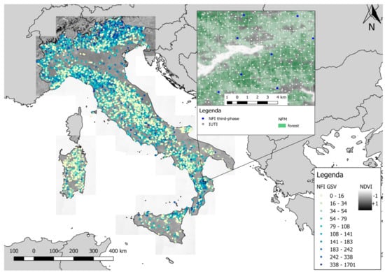
Figure 1.
The study area with the distribution of the national forest inventory (NFI) plots colored by growing stock volume (GSV) expressed in m3 ha−1. On the right, a detail of the distribution of sample points used in the study within the NFI 1 x 1 km grid where the third-phase NFI plots (Section 2.2.1) are depicted in blue and the Inventario dell’Uso delle Terre in Italia (IUTI) points (Section 2.2.2) in white.
The territory falls within the temperate zone of a Mediterranean climatic region (Pinna, 1970). On the coasts of the main islands, the average annual rainfall is 250 mm but reaches more than 3000 mm in the Alpine and pre-Alpine belts. Average yearly temperatures vary between 16 °C in the southern coastal areas to 10 °C in the inner central regions and the pre-Alps, with temperatures less than 5 °C in the mountain ranges and on the highest peaks.
According to the last Italian NFI (INFC, 2007), forest vegetation and other wooded lands occupy 10,467,533 ha, about 34% of the national territory. Forests are dominated by deciduous trees (68%), mainly Quercus oak (Q. petrea (M.) L., Q. pubescens W., Q. robur L., Q. cerris L.), and European beech (Fagus sylvatica L.). The dominant conifers are Norway spruce (Picea abies K.) and pines (Pinus sylvestris L., P. nigra A., P. pinae L., P. pinaster A.), which are mainly artificial plantations located in mountain areas or near the coast (Figure 1). Seven of the 14 European forest types occur in Italy, of which the most common is the thermophilous deciduous forest [14,57].
Italy is divided into 20 administrative regions (NUTS2) for each of which the NFI produces estimates of forest area, total and mean GSV, and their standard errors (SEs). The average GSV is 144 m3 ha−1 [58].
2.2. Field Data
2.2.1. Second Italian National Forest Inventory
The field reference data for the wall-to-wall spatial prediction of GSV were acquired in the framework of the second Italian NFI [59] based on a three-phase, systematic, unaligned sampling design with 1 × 1 km grid cells [60]. In the first phase, N = 301,300 points were selected and classified with respect to 10 coarse land-use strata using aerial orthophotos. In the second phase, for an n < N sub-sample of the points in the “forest” stratum of the first-phase points, qualitative information such as forest type, management, and property were collected during a field survey. In the third phase, for a sub-sample of 6782 points extracted from the second-phase points, a quantitative survey was carried out for circular plots of 13 m radius (530 m2). All tree stems with DBH of at least 2.5 cm were callipered, and for a subsample, height was measured. For all 6782 third-phase plots, allometric models [61] were used to predict GSV (m3) which was then aggregated at plot-level and scaled to a per unit area basis. For this study, allometric model prediction uncertainty and uncertainty due to Global Navigation Satellite System (GNSS) position error were expected to be negligible for the spatial resolution adopted [4,17,23,62]. The third-phase plots have mean GSV of 145.75 m3 ha−1, with median value of 102.82 m3 ha−1.
Official, design-based NFI estimates of total forest area and mean and total GSV at national and regional NUTS2 levels were acquired online at https://www.sian.it/inventarioforestale/ (accessed on: 2 October 2020) [62], for the reference year 2005.
The study area was tessellated into a 23 × 23 m national grid whose pixel area matched the area of the NFI ground plots, for a total of 569,769,690 pixels [19]. The national grid was used as a spatial reference grid for resampling the predictor variables and the FM to 23 × 23 m resolution.
2.2.2. Inventory of Land Use in Italy
To evaluate the accuracy of the FMs, we used the sample points from the Italian land use inventory (Inventario dell’Uso delle Terre in Italia, IUTI). The IUTI has adopted the methodology of approach number three of the Good Practices Guidance for Land Use, Land Use Change, and Forestry (GPG-LULUCF) of the Intergovernmental Panel on climate change [63,64,65]. IUTI is a permanent monitoring system that estimates the extent of six land use categories identified in the GPG-LULUCF. The IUTI is based on a systematic unaligned sampling design with 0.5 × 0.5 km grid cells which is an intensification of the NFI sample grid, for a total of 1,202,828 points of which 301,300 are the first-phase points of the NFI. The six categories reported by IUTI are urban, agriculture, forest land, grassland, wetland, other [65]. Each point is photo-interpreted in three time periods (1990, 2008, 2012) for estimating land-use change using aerial orthophotos with spatial resolution ranging between 1 × 1 m for 1990 and 0.5 × 0.5 m for 2008. We combined the six land use categories into forest and non-forest and assigned the value 1 to all the points classified as forest (class 1.1, 1.2) and 0 to all other categories. Subsequently, the forest class included 32% of the total observations with 387,085 of 1,202,818 points.
For this study, we used the IUTI points as an independent dataset to evaluate the accuracies of the FMs. We used the 2008 photointerpretation to be as consistent as possible with the 2005 NFI ground surveys.
2.2.3. Predictor Variables
To predict GSV as described in Section 3.1, we used predictors obtained from multiple sources including remotely sensed variables from multiple sensors, climate, and soil characteristics (Table 1). The variables were selected based on their availability throughout the national territory as reported by [17]. All variables were resampled from the original resolution to the 23 × 23 m pixel size of the national grid. A more detailed description of the database is provided by [17].

Table 1.
Predictor variables based on remotely sensed and auxiliary data.
2.2.4. Landsat Composite Image
We constructed a cloud-free composite image across Italy based on 848 Landsat 7 Enhanced Thematic Mapper Plus (ETM+) images acquired in the same year as the field survey (2005) +/− 1 year (Figure 2).
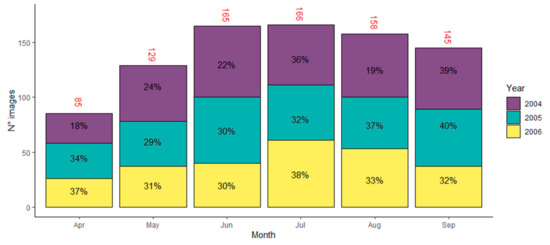
Figure 2.
Distribution of Landsat 7 ETM+ images per month, divided by acquisition years.
We used Landsat 7 Surface Reflectance Tier 1 imagery from the Earth Engine Data Catalog, acquired in the vegetation period (1 April–30 September), atmospherically corrected using Landsat Ecosystem Disturbance Adaptive Processing System LEDAPS [66]. We masked out cloud pixels based on the quality assessment (QA) band provided with the Landsat 7 database, using the C function of mask algorithm (CFMask) [67]. Finally, for each 23 × 23 m national grid pixel, we calculated the median values for each Landsat band [68].
2.2.5. SAR Variables
We used SAR data from PALSAR-2/PALSAR from the Advanced Land Observing Satellite (ALOS) and Advanced Land Observing Satellite-2 (ALOS-2) freely available at the global level online from the Japan Aerospace Exploration Agency (JAXA) at 25 × 25 m resolution. We rescaled the raw backscattering coefficients for each polarization HH and HV for the year 2007 to the 23 × 23 m pixel of the national grid. For more information on this data we refer to https://www.eorc.jaxa.jp/ALOS/en/palsar_fnf/fnf_index.htm (accessed on: 5 November 2019)
2.2.6. Climate and Soil Variables
We derived climate data from the 1 x 1 km downscaled climatological maps obtained by Maselli et al. [69] which is representative of the period 1981–2010. The dataset includes the following variables: total annual precipitation, mean annual temperature, maximum annual temperature, minimum annual temperature. For more details on these climate data, we refer to Chirici et al. [17].
Soil variables were from the harmonized soil geodatabase of Europe (European Soil Database v2.0—2004) [70]. The subsoil available water capacity and topsoil available water capacity soil variables used for this study were selected using the optimization phase described in Chirici et al. [17].
2.3. Forest Masks
We obtained five FMs available for the entire Italian territory that potentially reflect the forest FAO Forest Resource Assessment (FRA) definition [2]. These masks can be divided into two main categories: (i) FMs obtained by semi-automated classification of remotely sensed data; (ii) FMs obtained by manual delineation and classification of fine-resolution images. All the FMs were first reprojected in the WGS 84 / UTM zone 32 North (EPSG:32632) reference system to make them comparable and then resampled at the 23 × 23 m resolution of the national grid resulting to produce five comparable FMs.
2.3.1. National Forest Mask (NFM)
We used the national forest mask (NFM) which is based on the mosaic of local forest maps produced by manual photointerpretation by the Italian regional forest authorities [19]. The mosaic was constructed by merging 16 fine resolution forest maps with nominal reference scales varying between 1:5000 and 1:25,000 and five land use maps specifically filtered to produce forest cover maps. All the maps were based on manual photointerpretation of aerial orthophotos. The local forest maps were reclassified into Boolean masks using code 1 for pixels classified as “forest”, and code 0 for pixels classified as “non-forest”. The NFM is a mosaic of 20 fine-resolution regional forest maps resampled at the 23 × 23 m national grid resolution. The mask is also available on-line at www.forestinfo.it
2.3.2. Copernicus Land Monitoring System (CLMS) Forest Mask
To construct the Copernicus FM, we first used the 2012 Forest Type map (https://land.copernicus.eu/pan-european/high-resolution-layers/forests/forest-type-1/status-maps/2012?tab=download) (accessed on: 5 November 2020) that uses the Tree Cover Density layer (https://land.copernicus.eu/pan-european/high-resolution-layers/forests/tree-cover-density/status-maps/2012?tab=download) (accessed on: 5 November 2020) to classify all 20 × 20 m pixels of European lands as forest when the tree cover density is at least 10% and when such pixels are aggregated into a continuous patch of at least 0.52 hectares [46]. We excluded pixels in agricultural and urban contexts from the Forest Type map, using the Forest Additional Support Layer also available from Copernicus at https://land.copernicus.eu/pan-european/high-resolution-layers/forests/forest-type-1/status-maps/2012?tab=download (accessed on: 5 November 2020). The resulting map reflects as closely as possible the international forest definition in a raster layer having 23 × 23 m resolution
2.3.3. JAXA Forest Mask
JAXA constructed an FM for the reference years 2007 ± 1 with a spatial resolution of 25 × 25 m based on the HV-polarization backscatter images acquired by the PALSAR and PALSAR 2 sensors carried by the ALOS and ALOS2 satellites. JAXA adopted the FAO forest definition [47] and is available online at https://developers.google.com/earthengine/datasets/catalog/JAXA_ALOS_PALSAR_YEARLY_SAR (accessed on: 5 Novemeber 2020).
2.3.4. Hybrid Global Forest Mask 2000 (FM00)
Schepaschenko et al. [1] constructed a global FM using a hybrid approach combining multiple local, national, and global datasets into a single product. This map was constructed by converting the global forest probability map into a forest/non-forest map using a threshold calculated for each country. The threshold selected for this study produced area estimates that matched as closely as possible the official FAO forest area statistics. We characterized this map as “FM00”. The map has a spatial resolution of 1 × 1 km, was produced for the reference year 2000, and is available online at https://application.geo-wiki.org/branches/biomass/ (accessed on: 5 November 2020).
2.3.5. Corine Land Cover 2006 (CLC06)
The CORINE Land Cover (CLC) project was initiated in 1990 by the European Environmental Agency (EEA) [71] and has been updated in 2000, 2006, 2012, and 2018 to monitor land-use changes in the 39 participating countries [45]. It consists of land cover maps based on a nomenclature system of 44 classes produced by photointerpretation of fine-resolution satellite imagery. CLC uses a MMU of 25 hectares and a MMW of 100 m. For this study, we acquired the CLC map for the reference year 2006 ± 1 (referred to as “CLC06”) obtained by photo-interpretation of SPOT-4/5 and IRS P6 LISS III dual data images (EEA, 2007) [45] and available online in vector format at https://land.copernicus.eu/pan-european/corine-land-cover/clc-2006?tab=download (accessed on: 5 November 2020). To derive the CLC mask, we first rasterized the vector product to the 23 × 23 m spatial resolution of the national grid, and then we assigned the categories 2.4.4, 3.1.1, 3.1.2, 3.1.3, 3.2.3, 3.2.4 to the “forest” class and all the remaining categories to the “non-forest” class.
2.4. Overview of the Method
A concise overview of the methodology followed is presented: (i) a wall-to-wall GSV map was constructed using a random forests model with the NFI plot GSV data and the predictor variables; (ii) the accuracies of the five FMs were assessed; (iii) the wall-to-wall GSV map was masked in turn with each of the five FMs, obtaining five masked GSV maps; (iv) for each masked GSV map we estimated the mean and total GSV with the model-assisted regression estimator, at the national and regional levels; (v) we compared model-assisted estimations for each FM with the official estimate from the Italian NFI, in terms of correlation coefficient; (vi) we assessed the relationship between FM accuracies and GSV estimates in terms of the correlation coefficient.
2.5. Wall-to-Wall National GSV Map
To estimate the effects of FM accuracy on the model-assisted GSV estimates, we constructed a GSV map consisting of GSV predictions for all 23 × 23 m pixels of the national grid (569,769,690 pixels) using the random forests (RF) prediction technique with the NFI plot GSV data and the predictor variables described in Table 1. RF was optimized following Chirici et al. [17] by selecting the combination of predictor variables and parameter values (ntree and mtry) that minimized the root mean square error (RMSE) calculated using the leave one out cross-validation (LOOCV) technique [72]. RMSE was calculated as:
where n is the number of third-phase NFI plots (i.e., 6782), is the i-th GSV associated with the plots and is the i-th GSV predicted by the random forests model. The most accurate combination resulting from LOOCV was used to predict the GSV for all N pixels of the study area to produce a 23 × 23 m resolution GSV map. The model fitting and optimization phase was performed using the randomForest package within the statistical software package R 3.6.3 [73] (https://www.r-project.org, accessed on: 5 November 2020). For the 6782 NFI plots, the pixel-level GSV predictions ranged between 0 and 690 m3 ha−1 with a standard deviation of 68.5 m3 ha−1 while the original NFI values ranged between 0.3 and 701 m3 ha−1 with a standard deviation of 147 m3 ha−1. The map was found to have a mean deviation of −4.3 m3 ha−1.
2.6. Accuracy Assessment of FMs
We first assessed the five FMs with respect to thematic accuracy using the IUTI dataset as reference data. For each of the 1,202,828 points of the IUTI database, we extracted the forest/non-forest classification from the five FMs and constructed the respective five confusion matrices. For each matrix we calculated four metrics:
where:
for k categories and N observations.
These metrics need to be used together to correctly describe the quality of classification in the case of unbalanced datasets. This is the case for forest masks when the forest and non-forest classes cover the land area with very different proportions. In such cases, many classification performance indicators including overall accuracy may provide misleading information [74,75]. For this reason, the mask accuracy comparison should focus on recall as per Equation (6) and, most importantly, precision as per Equation (5).
2.7. Impact of FMs Accuracy on Model-Assisted GSV Estimation
The five FMs were used to mask out all non-forest pixels in the national GSV map. The pixel-level predictions for the resulting five masked GSV maps were used with a model-assisted, generalized regression estimator to infer mean and total GSV at both national (NUTS1) and regional levels (NUTS2) [20,21,22,23]. An initial estimate of GSV can be calculated from the masked GSV maps as,
where N is the number of forest pixels within the masked GSV map and is the GSV prediction obtained using the RF model for the i-th pixel. However, this estimator may be biased because of systematic prediction error. The bias can be estimated as,
where n is the NFI sample size, i.e., the number of plots used for constructing the model, is the GSV model prediction for the j-th plot and the observed value of GSV for the j-th plot. Subtracting the estimated bias from the initial estimate yields the model-assisted estimator as,
where ma denotes model-assisted, is the estimate of mean GSV for the given masked GSV map, N is the number of forest pixels within the masked GSV map, is the GSV prediction obtained using the RF model for the i-th pixel. The standard error (SE) for the estimator is:
where n is the NFI sample size, and
Similarly, the model-assisted estimator for the GSV total was:
where is the estimate of total GSV for the given GSV-masked map, N the number of pixels within the masked GSV map, the GSV prediction obtained using the RF model for i-th pixel. The SE for the is given by d’Oliviero et al. [76]:
where N is the population size, n is the NFI sample size, and
It is important to note that correction for estimated bias compensates for GSV map inaccuracy and makes the model-assisted estimator asymptotically unbiased.
Using the SEs, it was possible to construct confidence intervals for both estimates of mean and total GSV for the entire study area. These intervals are expressed as
where denotes either the model-assisted estimate of mean GSV or total GSV, is the SE of , and the factor tn depends on the desired significance level and the distribution of the response variable. For most distributions and applications, tn = 2 produces an approximate 95% confidence interval [23]. For purposes of constructing confidence intervals, the focus of the study was estimation of mean and total GSV and the SEs using the model-assisted regression estimators. To compare the GSV estimates produced with the five masked GSV maps and the NFI estimates at national and regional levels, we used the t statistic calculated as follows:
where denotes either the model-assisted estimate of mean GSV or total GSV for the masked GSV maps, denotes either the NFI estimate of mean GSV or total GSV, and and are the squares of the SEs of the estimates. Values of >2 indicate that the two estimates are statistically significantly different. Correlations for estimates of both mean and total estimates and the corresponding NFI estimates in terms of Pearson correlation coefficient (, ) were also calculated.
In addition, we calculated relative efficiency (RE) to assess the quality of the model-assisted estimators, compared to the SE obtained by the NFI [17], both at national and regional scales. RE was calculated as:
where and are the estimated variances of the NFI estimates and the model-assisted estimates, respectively.
Values of RE greater than 1.0 are evidence of greater precision in the model-assisted estimates [77]. RE could be interpreted as the factor by which the original sample size would have to be increased to achieve the same precision as that achieved using the remotely sensed auxiliary data [17].
Finally, we evaluated the relationship between the accuracies of the FMs (in terms of overall accuracy, κ, precision and recall) and the SEs of the model-assisted estimates for the NUTS2 administrative level using the Pearson correlation coefficient ().
3. Results
3.1. Forest Mask Accuracy Assessment
At the national level, the most accurate FM was the NFM with an underestimation against the NFI estimates of only −2%, followed by the CLC06 with −3%, JAXA with −4%, CLMS with +16%, and FM00 with +51%. The same ranking was obtained from the comparison with IUTI in terms of OA, κ, and precision (Table 2). For 17 of the 20 regions, the NFM was the most accurate, followed by the CLMS FM in two regions, and CLC06 in the remaining region. The confusion matrices for each one of the five FMs are shown in Figure 3.
Table 2.
Accuracy assessment for the five forest masks (FMs) based on the confusion matrices with the IUTI.
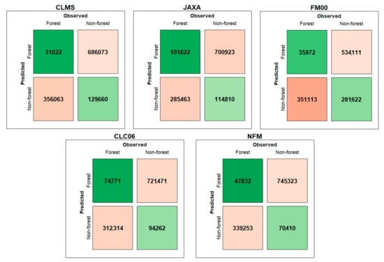
Figure 3.
Confusion matrices of each forest mask.
We also noted that regardless of the FM used, the islands (Sicilia and Sardegna) and some of the southern regions (Calabria, Campania, Puglia) were characterized by small precision and recall (sensitivity), leading to numerous misclassifications of non-forest as forest (commission errors) (Figure 4).
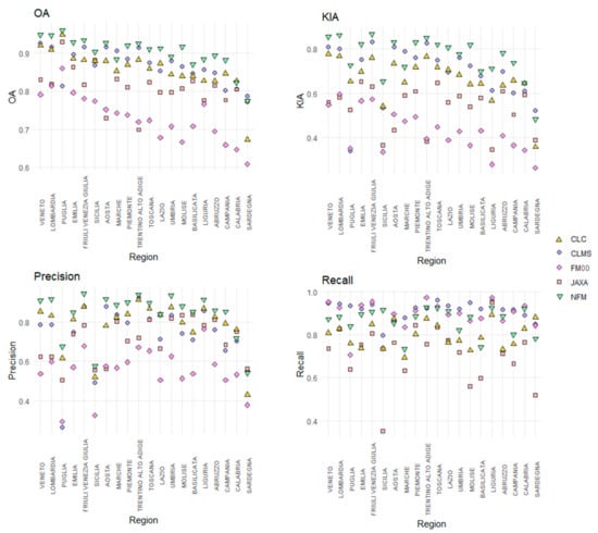
Figure 4.
Comparison of four accuracy metrics among the FMs, calculated at regional level (NUTS2).
3.2. GSV Model-Assisted Estimations
In Figure 5, the GSV map of Italy produced with the RF model is reported.
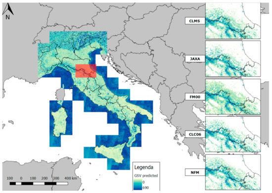
Figure 5.
Growing stock map of Italy generated with random forests model. GSV in m3 ha−1. On the right, a detail of the GSV map masked with the five forest masks.
For the five masked GSV maps, ranged between 125 (CLMS) and 135 (NFM), m3 ha−1 with between 1.1 and 1.3 m3 ha−1. For comparison, the design-based estimation of mean GSV from the NFI was 131 m3 ha−1 with SE of 1.6 m3 ha−1. Three of the five GSV-masked maps (NFM, CLC06, JAXA) produced estimates that were not statistically significantly different from the NFI estimate. The value of ranged between 1321 (JAXA) and 1525 (CLMS) millions m3, with between 13 (NFM) and 17 (JAXA) million m3, while the official estimate from the NFI was 1366 million m3 with SE of 14 million m3, demonstrating a general trend towards overestimation of total volume (Table 3). The differences between the total GSV estimate for two of the five masked GSV maps (NFM, CLC06) and the NFI estimate were not statistically significantly different from 0.
Table 3.
Model-assisted regression estimates for the five maps. The last row has the Italian NFI estimates.
For the 20 NUTS2 administrative regions, the greatest correlation with the NFI estimates was achieved by the GSV map masked with the NFM mask with = 0.972 and = 0.986 for the mean and total GSV, respectively (Table 4). The GSV maps masked with the CLMS and FM00 masks, despite their large values of , show a systematic overestimation of the .
Table 4.
Coefficient of correlation between the mean and total model-assisted estimate and NFI estimates for administrative NUTS2 regions (* p-value = 0; ** p-value < 0.001).
Regarding , for 16 of 20 regions, the differences between the model-assisted estimates and the NFI estimate were not statistically significantly different from 0 for the NFM masked GSV map, for 15 regions for CLMS and JAXA, for 14 regions for CLC06, and for 10 regions for FM00. Similar results were obtained for for which the differences for 16 of 20 regions were not statistically significantly different from 0 for the NFM masked GSV map, 15 for CLC06 and JAXA, six for CLMS, and two for FM00. The regions that always showed a statistically significant difference between the model-assisted estimates and the official NFI turned out to be the islands (Sardegna, Sicilia) and two regions (Puglia, Umbria), while those for which there were never significant differences were seven, distributed in northern and central Italy.
RE exceeded 1 for most regions, regardless of the FM used. RE < 1 was observed in one region for the CLMS and FM00 masks (Toscana), two regions for the CLC06 mask (Toscana, Emilia Romagna), and four regions for the JAXA mask (Toscana, Emilia Romagna, Sardegna, Umbria). The only masked GSV map that leads to RE coefficient always >1 was the NFM.
3.3. Relationship Between FMs Accuracy and GSV Estimates
The relationship between the accuracies of the FMs and the SEs of the estimates with the model-assisted estimator is presented in Table 5. The correlation was calculated for the 20 administrative regions.
Table 5.
Correlation coefficient between the accuracy metrics and the SEs of estimates for each FM. The overall values were calculated based on all five FMs together.
4. Discussion
The aim of this study was to assess the effects of using different FMs available for Italy for the area-based estimation of GSV. We first constructed a pixel-level GSV map for the entirety of Italy based on the procedure recently proposed by [17]. We then acquired five different FMs and, after evaluating their accuracies against an independent dataset (IUTI), we used them to mask out non-forest areas from the national GSV map produced with the random forest model. We then compared the five resulting model-assisted GSV estimates aggregated at regional levels with the official design-based NFI estimates.
Four of the five FMs achieved overall accuracies > 85%, based on the 2008 land use classification of IUTI points, with the CLC06 and NFM outperforming the other products. At the national level, the FM that achieved the greatest overall accuracy, κ and precision was the NFM, followed by the CLC06. Despite the greatest recall (0.91) achieved, the FM00 was affected by systematic overestimation of the regional forest area due to the original coarse resolution [1] which made this FM unsuitable for GSV estimation.
In contrast, the JAXA FM produced the smallest recall (0.74), most probably because the SAR backscatter in the HV polarization is relatively insensitive to Mediterranean vegetation [19,78] which probably caused an underestimation of the forest area. The photointerpreted FMs, CLC06 and NFM, had the greatest precision. This is an expected result because forest land use identification is typically done by local experts. However, CLC06 produced less precision than the NFM because it was implemented for monitoring land cover, not land uses, adopting a MMU and a crown cover threshold greater than that adopted by the INFC 2005 [53,79]. In fact, the CLC project did not map forest clear-cuts and other natural or anthropic disturbances as forest land use, but rather as bare soil or other non-forest classes, affecting the estimation of forest area. Conversely, the NFM, as a mosaic of local forest maps, is designed to monitor forest land use, such as the NFI. However, the small precision of the accuracy showed that false positives were the majority of classification errors.
At the regional level, OA was greater than 85% for 18 regions for the NFM mask, followed by the CLMS mask (14 regions), the CLC06 mask (12 regions), the JAXA mask (3 regions), and the FM00 mask (1 region). Regardless of the FM used, the greatest uncertainty was found in the southern regions and the islands (Campania, Calabria, Abruzzo, Basilicata, Sardegna, Sicilia), most probably because of the complex Mediterranean formations and complex agroforestry landscape tiles that characterized these regions where the NFI estimates also have larger associated SEs.
The greatest accuracies were achieved for regions characterized by greater forest cover (Liguria, Trentino-Alto Adige, Friuli-Venezia Giulia, Umbria, Toscana). These regions are characterized by extensive forests with continuous coverage and greater accumulation of GSV, as in the Apennine and Alpine Mountains, which probably reduces the likelihood of forest misclassifications, regardless of the FM considered.
Conversely, the forests bordering other land uses, along rivers, and in the coastal and rural contexts are typically characterized by a sparse canopy, which makes them more difficult to correctly classify, even by manual photointerpretation.
In conclusion, regarding the qualities of the FMs, the most accurate was the NFM, which was comparable with the CLC06, but with the advantage of a finer MMU which makes it more suitable for regional and local scale applications.
Regarding the model-assisted GSV estimates, although all the masked GSV maps overestimated total GSV, the NFM masked GSV map was most accurate as a trade-off between the national and regional GSV and the SE of estimates. The general overestimation was caused by the trend of the prediction model to overpredict GSV for pixels with small observed GSV values. (i.e., GSV < 250 m3 ha−1). This evidence, along with the limited GSV that characterizes Italian forests, caused the general overestimation at the national level. One possible solution is to increase the performance of the model, for example, by integrating ALS metrics which is a well-established data source for enhancing GSV predictions [8,13,15]. Both the CLMS and FM00 masked GSV maps suffered from systematic prediction error which caused the overestimation of , both nationally and regionally. For the CLMS masked GSV map, this can be caused by the inclusion of many agricultural and rural areas that occur in Italy [46], and for FM00 because of the original coarse spatial resolution (1 × 1 km). The differences between the model-assisted total GSV estimates and the official NFI estimate for two of the five masked GSV maps (NFM, CLC06) were statistically significantly different from 0. At the national level, the mean GSV estimates were comparable for all maps, except for the GSV map masked with the FM00 mask. The JAXA masked GSV map produced the same estimate as the NFI for mean GSV but underestimated the total due to the underestimation of forest area. However, the SEs were almost comparable for all the GSV-masked maps considered. The SE is mainly affected by the number of NFI plots used for building the model and calculation of the correction term in the estimator. Despite the differences among the FMs, the NFI plots falling within the forested portions of the FMs were similar, ranging between 6100 (CLMS) and 5800 (JAXA). Differences in the number of plots selected by each FM are likely to be concentrated at the forest edge, where maps are more prone to classification errors. These results confirm the findings of Esteban et al. [56], suggesting that the FM effects on area estimates are more important than the effects of field plot sampling variability on the uncertainty of the mean and total estimates.
At the regional level, the NFM produced the greatest relative to the NFI estimates, both for and , with the largest number of regional estimates in accordance with the NFI (16 regions out of 20). The NFM was also the only FM that led consistently to RE > 1. The CLC06 achieved similar results, with the major exception of Sardegna and in general in the southern regions, where, as we reported before, the MMU of the CLC project is not fine enough to discern the complex patchwork in the landscape of a rural region.
was smaller than for 16 regions, which represent 70% of the Italian territory. The regions with the greatest were Puglia, Valle d’Aosta, Molise, Basilicata, and Marche ( > 5%) probably because of the small number of NFI plots in these regions. Nevertheless, with the use of the model-assisted estimation approach, it was possible to decrease the error of the estimates with respect to the NFI estimates, both at the national (NUTS1), and regional levels (NUTS2).
Regarding the relationship between the FM accuracy and the SEs of the estimates, we found small correlation coefficients, in particular with the overall accuracy. The SE depends primarily on the sample size, which is less affected by the accuracy of the FMs, as reported by Esteban et al. [56]. The accuracy metric was more correlated with the SE of the estimates than was the recall, followed by the precision. This is an expected result because these metrics are strictly related to the area classified as forest which, in turn, affects the number of NFI plots included in the FMs. Of interest, the FM with the greatest recall (CLMS) was also the FM that included the greatest number of NFI plots.
However, the negative correlation with the other accuracy metrics demonstrated that a more accurate FM leads to a smaller .
It would be interesting to combine the available maps by aggregating their beneficial features to overcome the problems associated with each FM as per McRoberts et al. [23]. Another option would be to calibrate the FMs using the NFI data as per Næsset et al. [80].
In conclusion, the differences in the accuracies of the FMs led to different GSV estimates, although the SEs were almost comparable. The smallest GSV difference against the official NFI estimate was obtained by the most accurate FMs, i.e., the NFM. This is likely due to the correct classification of the main, dense forests, which have the largest amount of volume and subsequently make the greatest contribution in the model-assisted estimation. Presumably, forest misclassification occurs mainly along the margins and in boundary areas between different land uses.
5. Conclusions
This paper presents a comparative analysis of the impacts of different forest masks on model-assisted estimation of GSV. Several conclusions can be drawn from this study.
- At national and regional levels, the masked GSV map constructed using the NFM mask produced GSV estimates that were most similar to the official NFI estimates. Regardless of the forest mask, the major disagreement with the official estimate was found in the southern regions and islands, most probably because of the presence of the Mediterranean macchia, which is difficult to classify correctly, even by manual photointerpretation of fine-resolution images. These were the regions with the least classification accuracies. Regions with abundant forest components (central and northern regions) produced the most accurate masks and the most accurate and most precise GSV estimates.
- Despite the small correlation coefficients, we found a negative relationship between forest mask accuracy and the standard error of the GSV estimate, demonstrating that the accuracy of the FM must be considered in the GSV estimation through the model-assisted estimator.
- The quality of the model-assisted estimation mostly depends on the performance of the prediction model. A more accurate FM can compensate for systematic model prediction errors, leading to a greater agreement with official NFI GSV estimates, both at national and regional levels.
In conclusion, we recommend using the NFM, both at regional and national levels, for studies aimed at estimating forest parameters related to variables such as forest area, GSV, AGB, and carbon stock. However, it is plausible to assume that as the accuracy of the model predictions increases thanks to the growing availability of 3D data, the NFM will always produce more accurate and precise estimates of total GSV. In this regard, we hope that in the future, wall-to-wall ALS coverage will be finally available in Italy, to enhance the prediction of forest variables with even greater accuracy.
Finally, we strongly recommended that the different forest mapping and monitoring programs currently active in Italy converge on a common method and lead to harmonized, multiscale systems in line with the international forest definition.
Author Contributions
Conceptualization, G.C., E.V. and F.G.; methodology, E.V., G.D., S.F.; software, E.V.; validation, E.V.; formal analysis, E.V., G.D.; investigation, E.V., G.D.; resources, G.C., M.M. and B.L.; data curation, E.V., G.D.; writing—original draft preparation, E.V., G.C., R.E.M.; writing—review and editing, G.C., R.E.M., F.G., M.M. and B.L. All authors have read and agreed to the published version of the manuscript.
Funding
This research received no external funding.
Institutional Review Board Statement
Not applicable.
Informed Consent Statement
Not applicable.
Data Availability Statement
Data is contained within the article.
Conflicts of Interest
The authors declare no conflict of interest.
References
- Schepaschenko, D.; See, L.; Lesiv, M.; McCallum, I.; Fritz, S.; Salk, C.; Moltchanova, E.; Perger, C.; Shchepashchenko, M.; Shvidenko, A.; et al. Development of a global hybrid forest mask through the synergy of remote sensing, crowdsourcing and FAO statistics. Remote Sens. Environ. 2015, 162, 208–220. [Google Scholar] [CrossRef]
- FAO. Global Forest Resources Assessment 2010. Terms and Definition. Working paper 144/E. 2010. Available online: http://www.fao.org/3/am665e/am665e00.pdf (accessed on 7 October 2020).
- FAO; UNCCD. Sustainable Financing for Forest and Landscape Restoration: The Role of Public Policy Makers; FAO: Rome, Italy, 2015; p. 12. [Google Scholar]
- McRoberts, R.E.; Naesset, E.; Gobakken, T. Accuracy and Precision for Remote Sensing Applications of Nonlinear Model-Based Inference. IEEE J. Sel. Top. Appl. Earth Obs. Remote Sens. 2013, 6, 27–34. [Google Scholar] [CrossRef]
- Wittke, S.; Yu, X.; Karjalainen, M.; Hyyppä, J.; Puttonen, E. Comparison of two-dimensional multitemporal Sentinel-2 data with three-dimensional remote sensing data sources for forest inventory parameter estimation over a boreal forest. Int. J. Appl. Earth Obs. Geoinf. 2019, 76, 167–178. [Google Scholar] [CrossRef]
- Hansen, M.H.; Madow, W.G.; Tepping, B.J. An evaluation of model dependent and probability-sampling inferences in sample surveys. J. Am. Stat. Assoc. 1983, 78, 776–793. [Google Scholar] [CrossRef]
- McRoberts, R.E.; Tomppo, E.O. Remote sensing support for national forest inventories. Remote Sens. Environ. 2007, 110, 412–419. [Google Scholar] [CrossRef]
- Næsset, E.; Gobakken, T.; Holmgren, J.; Hyyppä, H.; Hyyppä, J.; Maltamo, M.; Nilsson, M.; Olsson, H.; Persson, Å.; Söderman, U. Laser scanning of forest resources: The nordic experience. Scand. J. For. Res. 2004, 19, 482–499. [Google Scholar] [CrossRef]
- Tomppo, E.; Olsson, H.; Ståhl, G.; Nilsson, M.; Hagner, O.; Katila, M. Combining national forest inventory field plots and remote sensing data for forest databases. Remote Sens. Environ. 2008, 112, 1982–1999. [Google Scholar] [CrossRef]
- Hollaus, M.; Dorigo, W.; Wagner, W.; Schadauer, K.; Höfle, B.; Maier, B. Operational wide-area stem volume estimation based on airborne laser scanning and national forest inventory data. Int. J. Remote Sens. 2009, 30, 5159–5175. [Google Scholar] [CrossRef]
- Waser, L.T.; Schwarz, M. Comparison of large-area land cover products with national forest inventories and CORINE land cover in the European Alps. Int. J. Appl. Earth Obs. Geoinf. 2006, 8, 196–207. [Google Scholar] [CrossRef]
- Waser, L.T.; Fischer, C.; Wang, Z.; Ginzler, C. Wall-to-Wall Forest Mapping Based on Digital Surface Models from Image-Based Point Clouds and a NFI Forest Definition. Forests 2015, 6, 4510–4528. [Google Scholar] [CrossRef]
- Kangas, A.; Astrup, R.; Breidenbach, J.; Fridman, J.; Gobakken, T.; Korhonen, K.T.; Maltamo, M.; Nilsson, M.; Nord-Larsen, T.; Næsset, E.; et al. Remote sensing and forest inventories in Nordic countries–roadmap for the future. Scand. J. For. Res. 2018, 33, 397–412. [Google Scholar] [CrossRef]
- White, J.C.; Coops, N.C.; Wulder, M.A.; Vastaranta, M.; Hilker, T.; Tompalski, P. Remote Sensing Technologies for Enhancing Forest Inventories: A Review. Can. J. Remote Sens. 2016, 42, 619–641. [Google Scholar] [CrossRef]
- Næsset, E. Area-Based Inventory in Norway–From Innovation to an Operational Reality. In Forestry Applications of Airborne Laser Scanning Concepts Case Study; Maltamo, M., Næsset, E., Vauhkonen, J., Eds.; Springer: Dordrecht, The Netherlands, 2014; pp. 215–240. [Google Scholar] [CrossRef]
- Puletti, N.; Floris, A.; Scrinzi, G.; Chianucci, F.; Colle, G.; Michelini, T.; Pedot, N.; Penasa, A.; Scalercio, S.; Corona, P.; et al. CFOR: A spatial decision support system dedicated to forest management in Calabria. For. Riv. Selvic. Ed Ecol. For. 2017, 14, 135–140. [Google Scholar] [CrossRef]
- Chirici, G.; Giannetti, F.; McRoberts, R.E.; Travaglini, D.; Pecchi, M.; Maselli, F.; Chiesi, M.; Corona, P. Wall-to-wall spatial prediction of growing stock volume based on Italian National Forest Inventory plots and remotely sensed data. Int. J. Appl. Earth Obs. Geoinf. 2020, 84, 101959. [Google Scholar] [CrossRef]
- Giannetti, F.; Puletti, N.; Puliti, S.; Travaglini, D.; Chirici, G. Modelling Forest structural indices in mixed temperate forests: Comparison of UAV photogrammetric DTM-independent variables and ALS variables. Ecol. Indic. 2020, 117, 106513. [Google Scholar] [CrossRef]
- D’Amico, G.; Vangi, E.; Francini, S.; Giannetti, F.; Nicolaci, A.; Travaglini, D.; Massai, L.; Giambastiani, Y.; Terranova, C.; Chirici, G. Are We Ready for a Web-Based National Forest Information System? State of the Art of for-Est Maps and Airborne Laser Scanning Data Availability in Italy. iForest. [CrossRef]
- Särndal, C.-E.; Swensson, B.; Wretman, J. Model Assisted Survey Sampling; Springer: New York, NY, USA, 1992; pp. 402, 694. [Google Scholar]
- Särndal, C.-E.; Swensson, B.; Wretman, J. Model Assisted Survey Sampling; Springer: Berlin, Germany, 2003; Available online: https://www.amazon.com/Assisted-Survey-Sampling-Springer-Statistics/dp/0387406204 (accessed on 6 November 2020).
- Breidt, F.J.; Opsomer, J.D. Chapter 27-nonparametric and semiparametric estimation in complex surveys. In Handbook of Statistics; Rao, C.R., Ed.; Elsevier: Amsterdam, The Netherlands, 2009; pp. 103–119. [Google Scholar] [CrossRef]
- McRoberts, R.E.; Vibrans, A.C.; Sannier, C.; Næsset, E.; Hansen, M.C.; Walters, B.F.; Lingner, D.V. Methods for evaluating the utilities of local and global maps for increasing the precision of estimates of subtropical forest area. Can. J. For. Res. 2016, 46, 924–932. [Google Scholar] [CrossRef]
- Næsset, E.; Gobakken, T. Estimation of above- and below-ground biomass across regions of the boreal forest zone using airborne laser. Remote Sens. Environ. 2008, 112, 3079–3090. [Google Scholar] [CrossRef]
- McRoberts, R.E. Probability- and model-based approaches to inference for proportion forest using satellite imagery as ancillary data. Remote Sens. Environ. 2010, 114, 1017–1025. [Google Scholar] [CrossRef]
- Giannetti, F.; Chirici, G.; Gobakken, T.; Næsset, E.; Travaglini, D.; Puliti, S. A new approach with DTM-independent metrics for forest growing stock prediction using UAV photogrammetric data. Remote Sens. Environ. 2018, 213, 195–205. [Google Scholar] [CrossRef]
- Goodbody, T.R.H.; Coops, N.C.; White, J.C. Digital Aerial Photogrammetry for Updating Area-Based Forest Inventories: A Review of Opportunities, Challenges, and Future Directions. Curr. For. Rep. 2019, 5, 55–75. [Google Scholar] [CrossRef]
- Barrett, F.; McRoberts, R.E.; Tomppo, E.; Cienciala, E.; Waser, L.T. A questionnaire-based review of the operational use of remotely sensed data by national forest inventories. Remote Sens. Environ. 2016, 174, 279–289. [Google Scholar] [CrossRef]
- Saarela, S.; Holm, S.; Grafström, A.; Schnell, S.; Næsset, E.; Gregoire, T.G.; Nelson, R.F.; Ståhl, G. Hierarchical model-based inference for forest inventory utilizing three sources of information. Ann. For. Sci. 2016, 73, 895–910. [Google Scholar] [CrossRef]
- Holm, S.; Nelson, R.; Ståhl, G. Hybrid three-phase estimators for large-area forest inventory using ground plots, airborne lidar, and space lidar. Remote Sens. Environ. 2017, 197, 85–97. [Google Scholar] [CrossRef]
- Nilsson, M.; Nordkvist, K.; Jonzén, J.; Lindgren, N.; Axensten, P.; Wallerman, J.; Egberth, M.; Larsson, S.; Nilsson, L.; Eriksson, J.; et al. A nationwide forest attribute map of Sweden predicted using airborne laser scanning data and field data from the National Forest Inventory. Remote Sens. Environ. 2017, 194, 447–454. [Google Scholar] [CrossRef]
- Immitzer, M.; Stepper, C.; Böck, S.; Straub, C.; Atzberger, C. Use of WorldView-2 stereo imagery and National Forest Inventory data for wall-to-wall mapping of growing stock. For. Ecol. Manag. 2016, 359, 232–246. [Google Scholar] [CrossRef]
- Karlson, M.; Ostwald, M.; Reese, H.; Sanou, J.; Tankoano, B.; Mattsson, E. Mapping tree canopy cover and above-ground biomass in Sudano-Sahelian woodlands using landsat 8 and random forest. Remote Sens. 2015, 7, 10017–10041. [Google Scholar] [CrossRef]
- Belgiu, M.; Drăguţ, L. Random forest in remote sensing: A review of applications and future directions. Isprs J. Photogramm. Remote Sens. 2016, 114, 24–31. [Google Scholar] [CrossRef]
- Stankiewicz, K.; Dąbrowska-Zielińska, K.; Gruszczynska, M.; Hoscilo, A. Mapping vegetation of a wetland ecosystem by fuzzy classification of optical and microwave satellite images supported by various ancillary data. In Proceedings of the Remote Sensing for Agriculture, Ecosystems, and Hydrology, Crete, Greece, 17 March 2003. [Google Scholar] [CrossRef]
- Hansen, M.C.; Potapov, P.V.; Moore, R.; Hancher, M.; Turubanova, S.A.; Tyukavina, A.; Thau, D.; Stehman, S.V.; Goetz, S.J.; Loveland, T.R.; et al. High-Resolution Global Maps of 21st-Century Forest Cover Change. Science 2013, 342, 850–853. [Google Scholar] [CrossRef]
- Dostálová, A.; Hollaus, M.; Milenković, M.; Wagner, W. Forest area derivation from sentinel-1 data. Isprs Ann. Photogramm. Remote Sens. Spat. Inf. Sci. 2016, III-7, 227–233. [Google Scholar] [CrossRef]
- Eysn, L.; Hollaus, M.; Schadauer, K.; Pfeifer, N. Forest Delineation Based on Airborne LIDAR Data. Remote Sens. 2012, 4, 762–783. [Google Scholar] [CrossRef]
- Dalponte, M.; Ørka, H.O.; Ene, L.T.; Gobakken, T.; Næsset, E. Tree crown delineation and tree species classification in boreal forests using hyperspectral and ALS data. Remote Sens. Environ. 2014, 140, 306–317. [Google Scholar] [CrossRef]
- Rudjord, O.; Trier, O.D. Tree species classification with hyperspectral imaging and lidar. In Proceedings of the 2016 8th Workshop on Hyperspectral Image and Signal Processing: Evolution in Remote Sensing (WHISPERS), Los Angeles, CA, USA, 12 February 2016; p. 4. [Google Scholar] [CrossRef]
- Øivind, D.T.; Salberg, A.-B.; Kermit, M.; Øystein, R.; Gobakken, T.; Næsset, E.; Aarsten, D. Tree species classification in Norway from airborne hyperspectral and airborne laser scanning data. Eur. J. Remote Sens. 2018, 51, 336–351. [Google Scholar] [CrossRef]
- Woodcock, C.E.; Allen, R.; Anderson, M.; Belward, A.; Bindschadler, R.; Cohen, W.; Gao, F.; Goward, S.N.; Helder, D.; Helmer, E.; et al. Free Access to Landsat Imagery. Science 2008, 320, 1011a. [Google Scholar] [CrossRef] [PubMed]
- Wulder, M.A.; Loveland, T.R.; Roy, D.P.; Crawford, C.J.; Masek, J.G.; Woodcock, C.E.; Allen, R.G.; Anderson, M.C.; Belward, A.S.; Cohen, W.B.; et al. Current status of Landsat program, science, and applications. Remote Sens. Environ. 2019, 225, 127–147. [Google Scholar] [CrossRef]
- Olofsson, P.; Arévalo, P.; Espejo, A.B.; Green, C.; Lindquist, E.; McRoberts, R.E.; Sanz, M.J. Mitigating the effects of omission errors on area and area change estimates. Remote Sens. Environ. 2020, 236, 111492. [Google Scholar] [CrossRef]
- European Enviromental Agency. Enviromental Statement; Office for Official Publications of the European Communities: Luxembourg, 2007; ISBN 978-92-9167-936-2. [Google Scholar]
- Langanke, T. Copernicus Land Monitoring Service–High Resolution Layer Forest: Product Specifications Document 38; Copernicus team at EEA, 2017; Available online: https://www.eea.europa.eu/data-and-maps/data/copernicus-land-monitoring-service-high (accessed on 5 November 2020).
- JAXA. Global 25m Resolution PALSAR-2/PALSAR Mosaic and Forest/Non-Forest Map (FNF) Dataset Description; Japan Aerospace Exploration Agency (JAXA), Earth Observation Research Center (EORC), 2016; Available online: https://www.eorc.jaxa.jp/ALOS/en/palsar_fnf/DatasetDescription_PALSAR2_Mosaic_FNF_revE.pdf (accessed on 5 November 2020).
- Seebach, L.; McCallum, I.; Fritz, S.; Kindermann, G.; LeDuc, S.; Böttcher, H.; Fuss, S. Choice of forest map has implications for policy analysis: A case study on the EU biofuel target. Environ. Sci. Policy 2012, 22, 13–24. [Google Scholar] [CrossRef]
- Fritz, S.; See, L. Comparison of land cover maps using fuzzy agreement. Int. J. Geogr. Inf. Sci. 2005, 19, 787–807. [Google Scholar] [CrossRef]
- Giri, C.; Zhu, Z.; Reed, B. A comparative analysis of the Global Land Cover 2000 and MODIS land cover data sets. Remote Sens. Environ. 2005, 94, 123–132. [Google Scholar] [CrossRef]
- Hoyos, A.P.; Rembold, F.; Kerdiles, H.; Gallego, J. Comparison of Global Land Cover Datasets for Cropland Monitoring. Remote Sens. 2017, 9, 1118. [Google Scholar] [CrossRef]
- Neumann, K.; Herold, M.; Hartley, A.; Schmullius, C. Comparative assessment of CORINE2000 and GLC2000: Spatial analysis of land cover data for Europe. Int. J. Appl. Earth Obs. Geoinf. 2007, 9, 425–437. [Google Scholar] [CrossRef]
- Seebach, L.M.; Strobl, P.; Miguel-Ayanz, J.S.; Gallego, J.; Bastrup-Birk, A. Comparative analysis of harmonized forest area estimates for European countries. Forests 2011, 84, 285–299. [Google Scholar] [CrossRef]
- Rodríguez-Veiga, P.; Saatchi, S.; Tansey, K.; Balzter, H. Magnitude, spatial distribution and uncertainty of forest biomass stocks in Mexico. Remote Sens. Environ. 2016, 183, 265–281. [Google Scholar] [CrossRef]
- Li, Z.-W.; Xin, X.-P.; Tang, H.; Yang, F.; Chen, B.-R.; Zhang, B.-H. Estimating grassland LAI using the Random Forests approach and Landsat imagery in the meadow steppe of Hulunber, China. J. Integr. Agric. 2017, 16, 286–297. [Google Scholar] [CrossRef]
- Esteban, J.; McRoberts, R.E.; Fernández-Landa, A.; Tomé, J.L.; Marchamalo, M. A Model-Based Volume Estimator that Accounts for Both Land Cover Misclassification and Model Prediction Uncertainty. Remote Sens. 2020, 12, 3360. [Google Scholar] [CrossRef]
- Barbati, A.; Marchetti, M.P.; Chirici, G.; Corona, P. European Forest Types and Forest Europe SFM indicators: Tools for monitoring progress on forest biodiversity conservation. For. Ecol. Manag. 2014, 321, 145–157. [Google Scholar] [CrossRef]
- Gasparini, P.; De Natale, F.; Di Cosmo, L.; Gagliano, C.; Salvadori, I.; Tabachi, G.; Tosi, V. INFC, 2009–I caratteri quantitativi–parte 1, vers. 2. In Inventario Nazionale delle Foreste e dei Serbatoi Forestali di Carbonio; MiPAAF–Ispettorato Generale Corpo Forestale dello Stato, CRA-MPF: Trento, Italy, 2009. [Google Scholar]
- INFC. Le stime di superficie 2005-seconda parte. In Inventario Nazionale delle Foreste e dei Serbatoi Forestali di Carbonio; Tabacchi, A.G., De Natale, F., Di Cosmo, L., Floris, A., Gagliano, C., Gasparini, P., Salvadori, I., Scrinzi, G., Tosi, V., Eds.; MiPAF–Corpo Forestale dello Stato-Ispettorato Generale, CRA-ISAFA: Trento, Italy, 2007; Available online: http://www.infc.it (accessed on 5 November 2019).
- Fattorini, L.; Marcheselli, M.; Pisani, C. A three-phase sampling strategy for large-scale multiresource forest inventories. J. Agric. Biol. Environ. Stat. 2006, 11, 296–316. [Google Scholar] [CrossRef]
- Tabacchi, G.; Di Cosmo, L.; Gasparini, P.; Morelli, S. Stima Del Volume E Della Fitomassa Delle Principali Specie Forestali Italiene, Equazioni Di Previsione, Tavole Del Volume E Tavole Della Fitomassa Arborea Epigea; Consiglio per la Ricerca e Sperimentazione in Agricoltura, Unità di Ricerca per Il Monitoraggio e la Pianificazione Forestale: Trento, Italy, 2011. [Google Scholar]
- McRoberts, R.E.; Chen, Q.; Walters, B.F.; Kaisershot, D.J. The effects of global positioning system receiver accuracy on airborne laser scanning-assisted estimates of aboveground biomass. Remote Sens. Environ. 2018, 207, 42–49. [Google Scholar] [CrossRef]
- Penman, J.; Gytarsky, M.; Hiraushi, T.; Krug, T.; Kruger, D.; Pipatti, R.; Buendia, L.; Miwa, K.; Ngara, T.; Tanabe, K.; et al. Good Practice Guidance for Land Use, Land Use Change and Forestry. Chapter 3: Annex 3A.1 Biomass Default Tables for Section 3.2 Forest Land Good Practice Guidance for Land Use, Land-Use Change and Forestry; The Institute for Global Enviromental Strategies for the IPCC and the Intergovernmental Panel on Climate Change, Hayama: Kanagawa, Japan, 2003; p. 21. [Google Scholar]
- Romano, D.; Arcarese, C.; Bernetti, A.; Caputo, A.; Condor, R.D.; Contaldi, M.; Lauretis, R.; Di Cristofaro, E.; Federici, S.; Gagna, A.; et al. Italian Greenhouse Gas Inventory 1990–2009. National Inventory Report; ISPRA: Rome, Italy, 2011. [Google Scholar]
- Corona, P.; Barbati, A.; Tomao, A.; Bertani, R.; Valentini, R.; Marchetti, M.; Fattorini, L.; Perugini, L. Land use inventory as framework for environmental accounting: An application in Italy. Iforest Biogeosci. For. 2012, 5, 204–209. Available online: http://www.sisef.it/iforest/contents?id=ifor0625-005 (accessed on 6 November 2020). [CrossRef]
- Masek, J.G.; Vermote, E.F.; Saleous, N.E.; Wolfe, R.; Hall, F.G.; Huemmrich, K.F.; Gao, F.; Kutler, J.; Lim, T.-K. A Land-sat surface reflectance dataset for North America, 1990–2000. IEEE Geosci. Remote Sens. Lett. 2006, 3, 68–72. [Google Scholar] [CrossRef]
- Foga, S.; Scaramuzza, P.L.; Guo, S.; Zhu, Z.; Dilley, R.D.; Beckmann, T.; Schmidt, G.L.; Dwyer, J.L.; Hughes, M.J.; Laue, B. Cloud detection algorithm comparison and validation for operational Landsat data products. Remote Sens. Environ. 2017, 194, 379–390. [Google Scholar] [CrossRef]
- Kennedy, R.E.; Yang, Z.; Gorelick, N.; Braaten, J.; Cavalcante, L.; Cohen, W.B.; Healey, S. Implementation of the LandTrendr Algorithm on Google Earth Engine. Remote Sens. 2018, 10, 691. [Google Scholar] [CrossRef]
- Maselli, F.; Pasqui, M.; Chirici, G.; Chiesi, M.; Fibbi, L.; Salvati, R.; Corona, P. Modeling primary production using a 1 km daily meteorological data set. Clim. Res. 2012, 54, 271–285. [Google Scholar] [CrossRef]
- Panagos, P. The European Soil Database; GEO, 2006; pp. 32–33. Available online: https://www.researchgate.net/publication/224842031_The_European_Soil_Database (accessed on 5 November 2020).
- Büttner, G.; Feranec, J.; Jaffrain, G.; Mari, L.; Maucha, G.; Soukup, T. The corine land cover 2000 project. EARSeL eProceedings 3, 3/2004 331. 2004. Available online: http://citeseerx.ist.psu.edu/viewdoc/download?doi=10.1.1.618.9940&rep=rep1&type=pdf (accessed on 6 February 2021).
- McRoberts, R.E.; Næsset, E.; Gobakken, T. Optimizing the k-Nearest Neighbors technique for estimating forest above-ground biomass using airborne laser scanning data. Remote Sens. Environ. 2015, 163, 13–22. [Google Scholar] [CrossRef]
- Liaw, A.; Wiener, M. Classification and regression by randomForest. Nucleic Acids Res. 2002, 5, 983–999. [Google Scholar] [CrossRef]
- Devarriya, D.; Gulati, C.; Mansharamani, V.; Sakalle, A.; Bhardwaj, A. Unbalanced breast cancer data classification using novel fitness functions in genetic programming. Expert Syst. Appl. 2020, 140, 112866. [Google Scholar] [CrossRef]
- Jaafor, O.; Birregah, B. KNN-LC: Classification in Unbalanced Datasets using a KNN-Based Algorithm and Local Centralities. In Data-Driven Modeling for Sustainable Engineering; Adjallah, K., Birregah, B., Abanda, H., Eds.; Springer: Cham, Switzerland, 2017; Volume 72. [Google Scholar] [CrossRef]
- D’Oliveira, M.V.; Reutebuch, S.E.; McGaughey, R.J.; Andersen, H.-E. Estimating forest biomass and identifying low-intensity logging areas using airborne scanning lidar in Antimary State Forest, Acre State, Western Brazilian Amazon. Remote Sens. Environ. 2012, 124, 479–491. [Google Scholar] [CrossRef]
- Moser, P.; Vibrans, A.C.; McRoberts, R.E.; Næsset, E.; Gobakken, T.; Chirici, G.; Mura, M.; Marchetti, M. Methods for variable selection in LiDAR-assisted forest inventories. Forestry 2016, 90, 112–124. [Google Scholar] [CrossRef]
- Bartsch, A.; Widhalm, B.; Leibman, M.; Ermokhina, K.; Kumpula, T.; Skarin, A.; Wilcox, E.J.; Jones, B.M.; Frost, G.V.; Höfler, A.; et al. Feasibility of tundra vegetation height retrieval from Sentinel-1 and Sentinel-2 data. Remote Sens. Environ. 2020, 237, 111515. [Google Scholar] [CrossRef]
- Vizzarri, M.; Chiavetta, U.; Chirici, G.; Garfì, V.; Bastrup-Birk, A.; Marchetti, M. Comparing multisource harmonized forest types mapping: A case study from central Italy. Iforest-Biogeosci. For. 2015, 8, 59–66. Available online: http://www.sisef.it/iforest/contents/?id=ifor1133-007 (accessed on 5 November 2020). [CrossRef]
- Næsset, E. Airborne laser scanning as a method in operational forest inventory: Status of accuracy assessments accom-plished in Scandinavia. Scand. J. For. Res. 2007, 22, 433–442. [Google Scholar] [CrossRef]
Publisher’s Note: MDPI stays neutral with regard to jurisdictional claims in published maps and institutional affiliations. |
© 2021 by the authors. Licensee MDPI, Basel, Switzerland. This article is an open access article distributed under the terms and conditions of the Creative Commons Attribution (CC BY) license (http://creativecommons.org/licenses/by/4.0/).