Article

Evaluation of Three Different Machine Learning Methods for Object-Based Artificial Terrace Mapping—A Case Study of the Loess Plateau, China

1
School of Geography, South China Normal University, Guangzhou 510631, China
2
Key Laboratory of Virtual Geographic Environment, Ministry of Education, Nanjing 210023, China
3
College of Civil Engineering, Nanjing Forestry University, Nanjing 210037, China
4
Nanjing Institute of Geography and Limnology, Chinese Academy of Sciences, Nanjing 211100, China
5
Key Laboratory of Watershed Geographic Sciences, Nanjing Institute of Geography and Limnology, Chinese Academy of Sciences, Nanjing 210008, China
6
School of Geography, Nanjing Normal University, Nanjing 210023, China
7
Jiangsu Center for Collaborative Innovation in Geographical Information Resource Development and Application, Nanjing 210023, China
*
Author to whom correspondence should be addressed.
Remote Sens. 2021, 13(5), 1021; https://doi.org/10.3390/rs13051021
Submission received: 27 January 2021 / Revised: 26 February 2021 / Accepted: 6 March 2021 / Published: 8 March 2021

Abstract

:
Artificial terraces are of great importance for agricultural production and soil and water conservation. Automatic high-accuracy mapping of artificial terraces is the basis of monitoring and related studies. Previous research achieved artificial terrace mapping based on high-resolution digital elevation models (DEMs) or imagery. As a result of the importance of the contextual information for terrace mapping, object-based image analysis (OBIA) combined with machine learning (ML) technologies are widely used. However, the selection of an appropriate classifier is of great importance for the terrace mapping task. In this study, the performance of an integrated framework using OBIA and ML for terrace mapping was tested. A catchment, Zhifanggou, in the Loess Plateau, China, was used as the study area. First, optimized image segmentation was conducted. Then, features from the DEMs and imagery were extracted, and the correlations between the features were analyzed and ranked for classification. Finally, three different commonly-used ML classifiers, namely, extreme gradient boosting (XGBoost), random forest (RF), and k-nearest neighbor (KNN), were used for terrace mapping. The comparison with the ground truth, as delineated by field survey, indicated that random forest performed best, with a 95.60% overall accuracy (followed by 94.16% and 92.33% for XGBoost and KNN, respectively). The influence of class imbalance and feature selection is discussed. This work provides a credible framework for mapping artificial terraces.

Graphical Abstract

1. Introduction

Artificial terraces, as a typical artificial landform, are of great importance to agricultural production and soil and water conservation [1]. The construction of artificial terraces enhances water infiltration, reduces the risk of soil erosion, and improves biodiversity [2,3]. Artificial terraces are widely distributed around the world because of these advantages [4]. Many previous studies reported their effects on soil and water processes [5,6,7]. Nowadays, many artificial terraces are threatened by land degradation and soil erosion because of land abandonment and a lack of maintenance [8]. The Loess Plateau in China, which is a major agricultural production region in China, suffers from severe soil erosion and is a fragmented terrain [9]. Since the 1960s, lots of artificial terraces have been built on the top of the loess hills and hillslopes to improve agricultural productivity. However, the “Grain for Green” project was implemented by the Chinese government in 1999, with the aim to “convert all reclaimed farmland to forestland step by step within a definite time in a planned way” [10]. Through this project, hillsides were closed to actively facilitate afforestation, the ecological environment was improved, and vegetation recovery was accelerated [11]. Currently, the terraces are consistently at risk from gully erosion or gravity erosion because of the lack of maintenance [12,13]. The evident changes in certain artificial terrace areas can be clearly observed (Figure 1). Hence, mapping artificial terraces will help us better understand their spatial distribution and other effects, such as geomorphology, soil erosion, and ecology.
Terrace mapping is the basis of this field of study. Traditional methods, including field investigation and visual interpretation [14,15], are simple, highly accurate, and easy to implement. However, the time expenditure, financial costs, and inconvenience make long-term monitoring over large areas difficult. Automatic methods are possible with the technological development of high spatial resolution remote sensing and terrain modeling by unmanned aerial vehicle (UAV) photogrammetry [16,17,18] or light detection and ranging (lidar) technology [8]. Highly accurate terrain modeling by UAV photogrammetry is consistently difficult because fully and automatically interpolating the surface model into the terrain model, i.e., the digital elevation model (DEM), is problematic in hilly areas covered with dense vegetation [19]. The DEM-based mapping method is usually influenced by elevation noises caused by vegetation or other features. Lidar-based terrain modeling usually solves this problem using the multiple echo filtering technique, while the high economic cost limits its application. However, image-based methods utilize spectrum information and can achieve a better result. These methods include two types: pixel-based [16,20,21] and object-based methods [22].
Object-based image analysis (OBIA) transfers from pixels to objects [23]. Therefore, spectral as well as spatial information of target features [24] can be better utilized for the mapping task. This characteristic makes OBIA superior to pixel-based methods, which usually ignore these contents and texture information, leading to a discontinuity of mapping results. A general OBIA framework basically consists of three steps. First, an image is segmented into several individual polygons with approximately the same spectral or spatial features, namely, objects. Then, each object is treated as the analysis unit, and the corresponding features are calculated for incoming classification. Finally, a specific classifier is selected to achieve a certain classification task. The first step in OBIA, i.e., image segmentation, can directly affect the analysis [25]. Commonly-used segmentation methods, such as multi-resolution segmentation (MRS) implemented in eCognition software [26,27,28], are strongly defined by the parameters (scale, shape, and compactness in this MRS). Therefore, the inherent properties of geographic entities are necessity as the prior knowledge to obtain suitable segmentations.
Another significant factor affecting the efficiency of the OBIA framework is the application of the appropriate classifier. Previous studies have successfully utilized machine learning (ML) classifiers to classify highly complex data, which illustrate the great potential of ML in effective classification and object recognition [29]. Zhao et al. (2017) proposed a random forest-based method using DEMs and UAV imagery for terrace mapping with an overall accuracy of 94% [22]; however, the geometric features of terraces were not considered, which limits the accuracy. Dai et al. (2020) used edge detection combined with terrain attributes to extract the ridge lines of artificial terraces with an overall accuracy of 90.81%–97.57% [13]. While the inconsistency caused by soil erosion between terrace ridges will strongly influence the success of this method, among the various existing ML-based classifications, ensemble decision tree (DT) classifiers, such as random forest (RF), are considered as effective methods for mapping purposes in remote sensing. Recently, as a novel state-of-the-art DT-based ensemble classifier, extreme gradient boosting (XGBoost) is reported as a strong and effective method that has been successfully used for OBIA-based classification, such as landscape classification and gully feature mapping [25]. However, the capabilities of XGBoost for artificial terrace mapping remain to be demonstrated. Moreover, other algorithms under the OBIA framework are also commonly used for remote sensing classification, such as k-nearest neighborhood (KNN) [30]. Although a few studies have focused on the comparison of ML performance in land use and land cover [31] or natural hazard susceptibility (e.g., landslide) mapping [32,33,34], no comprehensive comparison with fine-scale artificial terrace mapping has been performed with an OBIA framework.
Considering the aforementioned limitations, this work focuses on the comparison of different ML classifiers in the OBIA framework for artificial terrace mapping. The contributions to this field are as follows: 1) image segmentation was optimized and feature selection was performed with an objective method; 2) the performance of three ML classifiers in the OBIA framework was compared and their potential for artificial terrace mapping was explored.

2. Materials and Methods

2.1. Study Area and Data

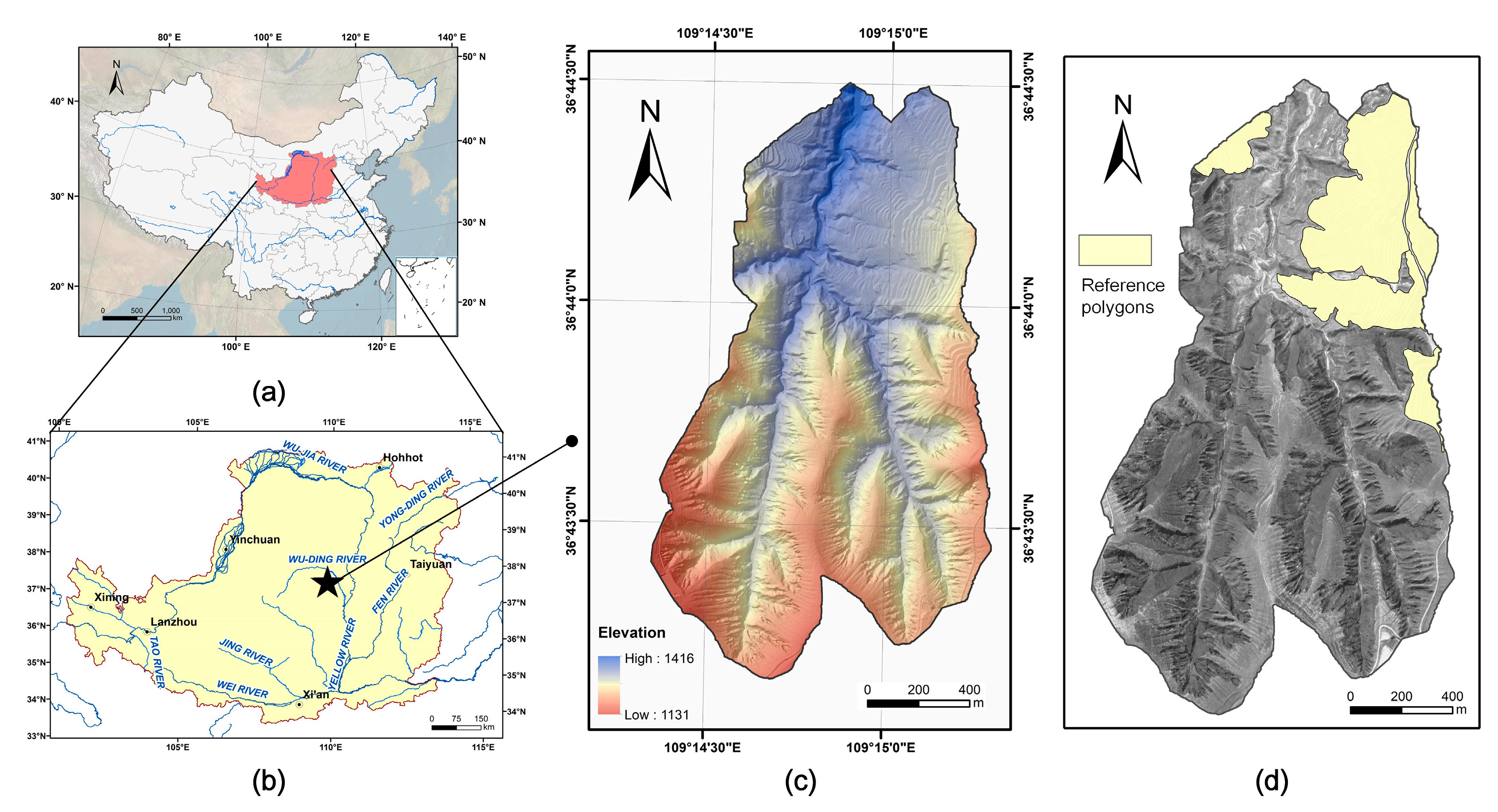
The Zhifang catchment (109°14′25″E–109°15′20″E, 36°43′10″N–36°44′30″N, with an area of 2.33 km2) was selected as the study area (Figure 2a,b). It is located in the southeastern part of Ansai County, Shaanxi Province, China. The study area is composed of loess ridge and hill, with a 289-m elevation difference, and is covered with massive ridges and tablelands. The study area is characterized by a semiarid climate with mean annual precipitation of 528.5 mm and a mean temperature of 8.8 °C [35,36,37]. Soil erosion is evidently severe, with a great number of artificial terraces built in this area, making the terrain fragmented.
In this study, high-resolution DEMs and imagery were used to extract the terraces. A DEM with a 1-m resolution was generated using UAV photogrammetry in March 2016 (Figure 2c). DEM acquisition can be divided into two main phases: the outdoor field survey and subsequent indoor image processing. For the outdoor survey, two steps are needed. First, an MD4-1000 drone with a Sony ILCE-7R digital camera system was used to capture optical aerial photographs of the study site. Secondly, the horizontal and vertical accuracies were maintained based on three base control points and 53 photo control points. Then, two indoor image processing steps were implemented: aerial triangulation and DEM generation. Trimble’s Inpho 6.0 was used to perform the aerial triangulation. Subsequently, the DSM was generated using MapMatrix 4.0. Then, a 1-m resolution DEM was achieved after eliminating buildings and vegetation. The WorldView-3 imagery from April 2016 (Figure 2d) was utilized in this study. Launched in August 2014, the WorldView-3 satellite has higher spatial resolution than the previous WorldView-2 satellite. The resolution of the panchromatic band is 0.31 m, and the multispectral (red, green, blue, and near-infrared) bands are 1.24 m.
A field investigation was then conducted to generate the ground truth of the artificial terraces to evaluate the mapping accuracy. Reference polygons (Figure 2d) were manually delineated from both the field investigation and the details of the terrace based on WorldView-3 Imagery, DEM information, and Ortho-image (Figure 3).

2.2. Methods

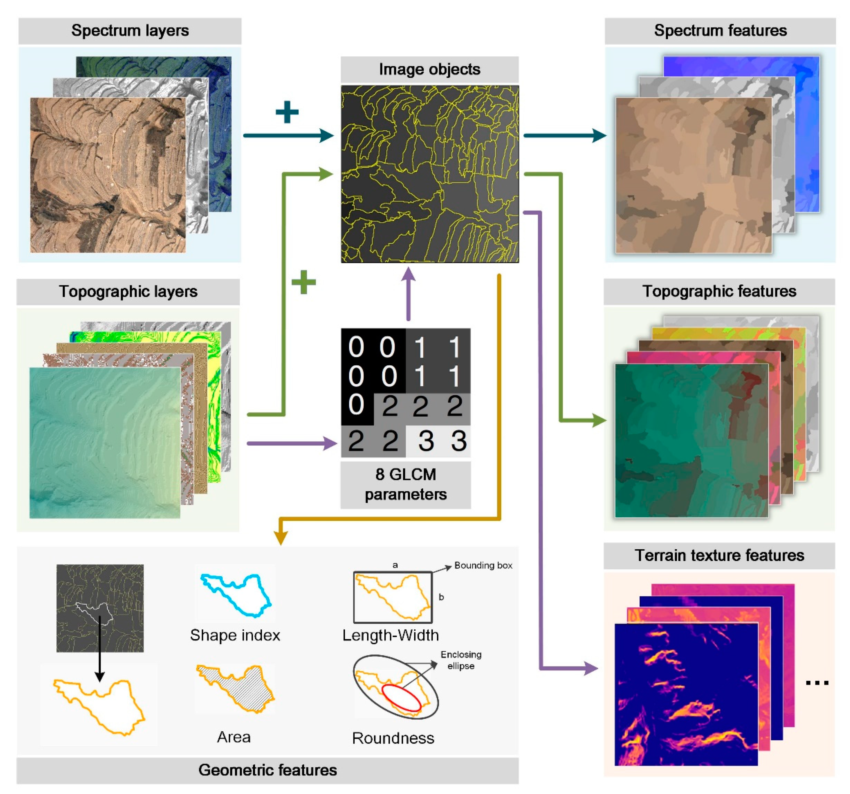
The mapping task began with image segmentation, which is an essential step that affects the accuracy of terrace mapping. In this study, segmentation by weighted aggregation (SWA) was utilized for this step because it can generate multiple level segments without many predefined parameters. Subsequently, a watershed-based optimization strategy was initiated to optimize the segmentation. Then, the spectrum, topography, terrain texture, and geometry were calculated for each suitable segment. Next, a correlation-based feature selection method was adopted to acquire the relevant feature subsets. Subsequently, three object-based ML classifiers, namely, RF, XGBoost, and KNN, were selected for terrace mapping. Finally, the mapping results were validated and compared through an accuracy assessment analysis. Figure 4 illustrates the entire workflow of this study.

2.2.1. Optimized Image Segmentation

SWA, firstly proposed by Sharon et al. (2000, 2001, 2006) [38,39,40], mainly consists of four steps: (1) constructing the fine-level graph; (2) creating the coarse-level graph; (3) evaluating the saliency of segments; and (4) determining the boundaries of salient segments based on a top-down procedure. In this study, the SWA was used to obtain the multi-level segmentation results based on three visible bands, one near-infrared band, and one panchromatic band. Then, the segments were used as the basic processing units for terrace mapping. Therefore, selecting an appropriate level segmentation from multi-level results is necessary to optimize the segments that are generated by SWA. Present studies have pointed out that the category’s effect on the segmentation selection needs to be considered [30]. This finding indicates that using different levels to segment an image is better than using a universal one [29]. In order to achieve a satisfactory segmentation, it is necessary to consider the homogeneity of segments and significant difference with the adjacent regions [41]. Hence, a watershed-based optimized strategy was used to select the optimal segmentation level on the basis of our previous knowledge [25]. This procedure first chooses the watershed as the basic processing unit because it is usually considered as the fundamental unit of landform [42]. The three following steps are used to extract sub-watersheds: (1) filling the sinks; (2) extracting the stream network; and (3) extracting the watersheds. Eighteen sub-watersheds were extracted; two were used for model training, with the remaining 16 sub-watersheds being utilized for validation. Every sub-watershed has its own segmentation level by considering between-segment heterogeneity and within-segment homogeneity [43]. To meet these requirements, an unsupervised F-measure was utilized [44]. Subsequently, the optimized segmentation level of each sub-watershed was achieved, and the final segmentation result was obtained.

2.2.2. Feature Extraction and Selection

For the ML-based terrace mapping, certain features need to be extracted to train the classifiers. In this study, 55 features were adopted for training the terrace mapping model. An overview of these features is illustrated in Table 1. The detailed descriptions for each feature can be found in Appendix A. Given that the spectrum and geometric features are widely used in the OBIA community [25], this information was used. Five basic topographic factors, namely, elevation, slope, roughness, shaded relief, and curvature, were utilized. Terrain textures, which are beneficial for the extraction of landform entities [45,46], were also adopted. Eight terrain texture measures derived from the gray-level co-occurrence matrix (GLCM) [47] were then calculated on the basis of five topographic features. All these object features were calculated based on the segmentation result using the eCognition software. Figure 5 illustrates the schematic for object-based feature extraction.
A correlation-based feature selection (CFS) method [48], which is a popular filter approach, was used to select the feature subset in terrace mapping in this study. In this method, the feature subsets were evaluated by maximizing the dependency of a feature subset with the target class while minimizing the intercorrelation within the subset [49]:
f ( S ) = SC i ASC i
where S denotes a candidate feature subset, f ( S ) denotes the evaluation score, SC i denotes the average correlation between subset S and the dependent variable, and ASC i denotes the average intercorrelation within subset S. Given an initial set of inputs, a set of features meeting the best f ( S ) was identified. Each time the feature set proposed by the CFS was removed from the initial input, the algorithm was then reapplied to the set of reduced variables until no features were left. This selection algorithm in this work was implemented using the Weka 3.8 package.

2.2.3. Terrace Mapping Using ML Classifiers

After image segmentation and feature selection, three different widely-used ML classifiers, namely, XGBoost, RF, and KNN, were selected for terrace mapping.
(I) XGBoost
XGBoost [50], as a boosting-based ensemble classifier, serially trains individual DTs, and each DT is an improved version of the previous one, resulting in a smaller error rate [51]. This serialized training method is beneficial to reduce the residuals. To avoid overfitting the model, XGBoost adds a regularization term to the objective function for controlling the entire complexity of the model [52]. Another significant enhancement of XGBoost is the parallel processing ability. The algorithm uses presorting and block storage methods to determine the best split point rather than growing the DT in parallel. Then, linear scanning can be performed across the blocks to determine where the best split point is for each feature under test. Such characteristics make XGBoost very popular for the classification and mapping of remote sensing images.
In this study, the “XGBoost” package [53] in R language was employed to generate the terrace mapping model. For the sake of modeling, three significant parameters need to be determined: (1) the number of trees (nrounds) to grow; (2) the depth of the trees (max_depth), which controls the complexity of the model; and (3) the minimum sum of the instance weight (min_child_weight), which determines the stop point of the tree splitting. For tuning the XGBoost model, 10-fold cross-validation was selected on the training dataset.
(II) RF
RF is another type of ensemble classifier, proposed by Leo Breiman in 2001 [54]. It uses bagging to generate different training samples to reduce the correlation between classification models, thereby improving the overall prediction accuracy of the classifier. The classification process of RF is simple and easy to implement. The training samples are randomly and repeatedly selected from the original training set through bootstrap sampling. Every classification and regression tree (CART) DT is based on every bootstrap dataset and is split and grown by independently and identically distributed random vectors. The final classification result is synthesized from the classification results trained by each CART DT through simple majority voting.
We used the R language to implement the RF package and build the terrace mapping model. Two important parameters affect the model performance, namely, the number of trees (nTree) needed to be grown and the number of features (mTry) that are randomly selected at each node. The nTree and mTry were set to 500 and the square root of the total number of features because they are a commonly used parameter combination for RF classifier [55].
(III) KNN
KNN is a powerful tool used in many object-based procedures [56,57] because of its flexibility and simplicity. This classification method is frequently utilized in object-based software frameworks. Compared with model-based learning, KNN assigns objects to classes on the basis of the proximity or neighborhood in feature space rather than learning from models [58]. The nearest K neighbors can be achieved from the training data and used to vote for the new target prediction [59]. In this study, KNN was adopted using the eCognition software (Trimble Geospatial, Munich, Germany).

2.2.4. Mapping Accuracy Assessment

After the terraces were predicted, the predicted results were validated on the basis of the reference data. In this study, precision (Pr), recall (Re), F1-score (F1), overall accuracy (OA), and kappa coefficient (k) were adopted for the accuracy assessment. These metrics can be calculated as follows:
Pr = TP TP + FP
Re = TP TP + FN
F 1 = 2 × Pr × Re Pr + Re
OA = TP + TN TP + FP + TN + FN
k = P 0 P e 1 P e
where Po is the overall accuracy, and Pe can be defined as
P e = ( TP + FP ) ( TP + FN ) + ( FN + TN ) ( TN + FP ) ( TP + FP + TN + FN ) 2
where TP, FP, and FN denote true positive, false positive, and false negative, respectively. TP refers to the terrace area for which the extraction result is correct. FP refers to the terrace area for which the extraction result is incorrect. FN refers to the terrace area that has not been extracted. Therefore, the Pr metric indicates to what extent the extraction result represents the real target terrace area, and the Re metric indicates to what extent the real target can be extracted. The former metric can characterize the classification commission error of the model, and the latter can represent the omission error. F1 is the harmonic mean of the two metrics, reflecting their balance. Thus, it is used to characterize the OA of the model [60].

3. Results and Analysis

3.1. Image Segmentation and Feature Selection Results

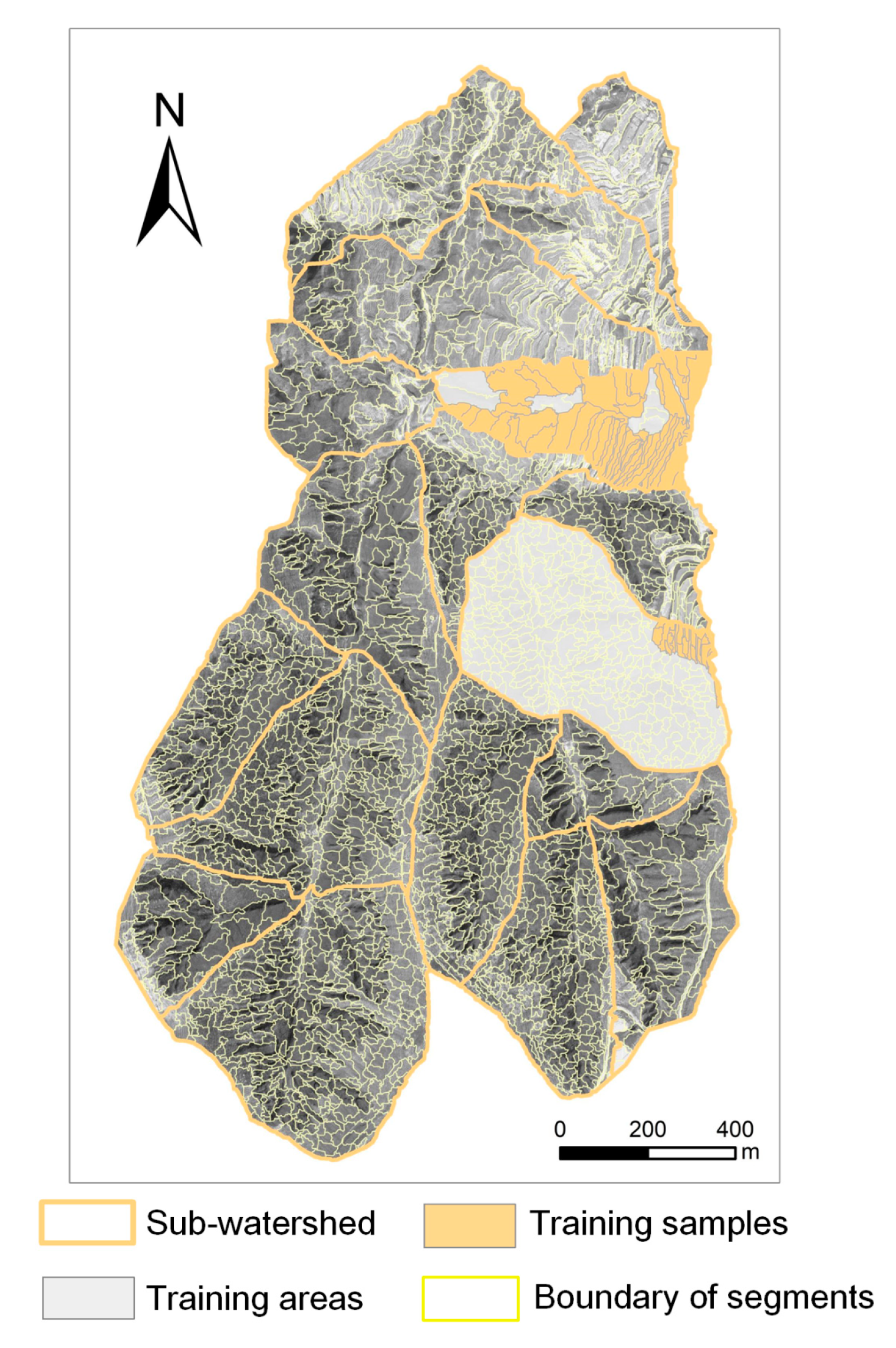
The segmentation result can be achieved using the watershed-based SWA optimization strategy, as presented in Figure 6. In accordance with the segmentation results, 18 sub-watersheds and 3445 segments were generated. Two sub-watersheds were selected to train the ML models. The training area consists of 849 segments, including 78 positive samples and 731 negative samples. They were used to train the terrace mapping model. The remaining 16 sub-watersheds (2596 segments) were used to validate the model. For selecting the relevant feature subset, 20-fold replicate runs of the CFS method were implemented. The top 20 features were chosen, as shown in Table 2. The GLCM-based terrain texture can fully consider the spatial relationship among pixels, thereby providing the terrain texture a reliable basis for reflecting the assemblages of repeating patterns of landform elements [61]. Therefore, the terrain texture features play a dominant role in feature ranking. Eleven terrain texture features were selected. The terrain texture based on GLCM can be regarded as a second-order geomorphic parameter. These second-order parameters can improve the ability of traditional terrain factors to differentiate landform types. The GLCM angular second moment measures the uniformity of the texture feature. The smaller the value is, the more disorderly the image pixels will be. Therefore, the angular second moment of curvature (Ang_Cur) can be used to reflect the internal change pattern for the curvature. The larger the value of Ang_Cur, the more orderly the curvature, indicating that the change in the curvature is gentle. Given that the curvature measures the convexity of the landscape, a small Ang_Cur likely represents a complicated area. These areas usually have great potential to develop bank gullies. Therefore, compared with the traditional topographic features, terrain textures can preferably distinguish differences in landforms on a certain scale [52]. In addition to terrain texture features, three geometric and two topographic features were selected in the ranking list, indicating that they do not have a great deal of influence in terms of improving the accuracy of terrace mapping. The Pan feature ranks in the top positions, as shown in Table 2. This condition might be attributed to the high spatial resolution of the panchromatic band with a 0.31-m resolution. Thus, the features obtained from the panchromatic band are more important than those from the 1-m resolution DEM.

3.2. Terrace Mapping Results and Accuracy Assessment

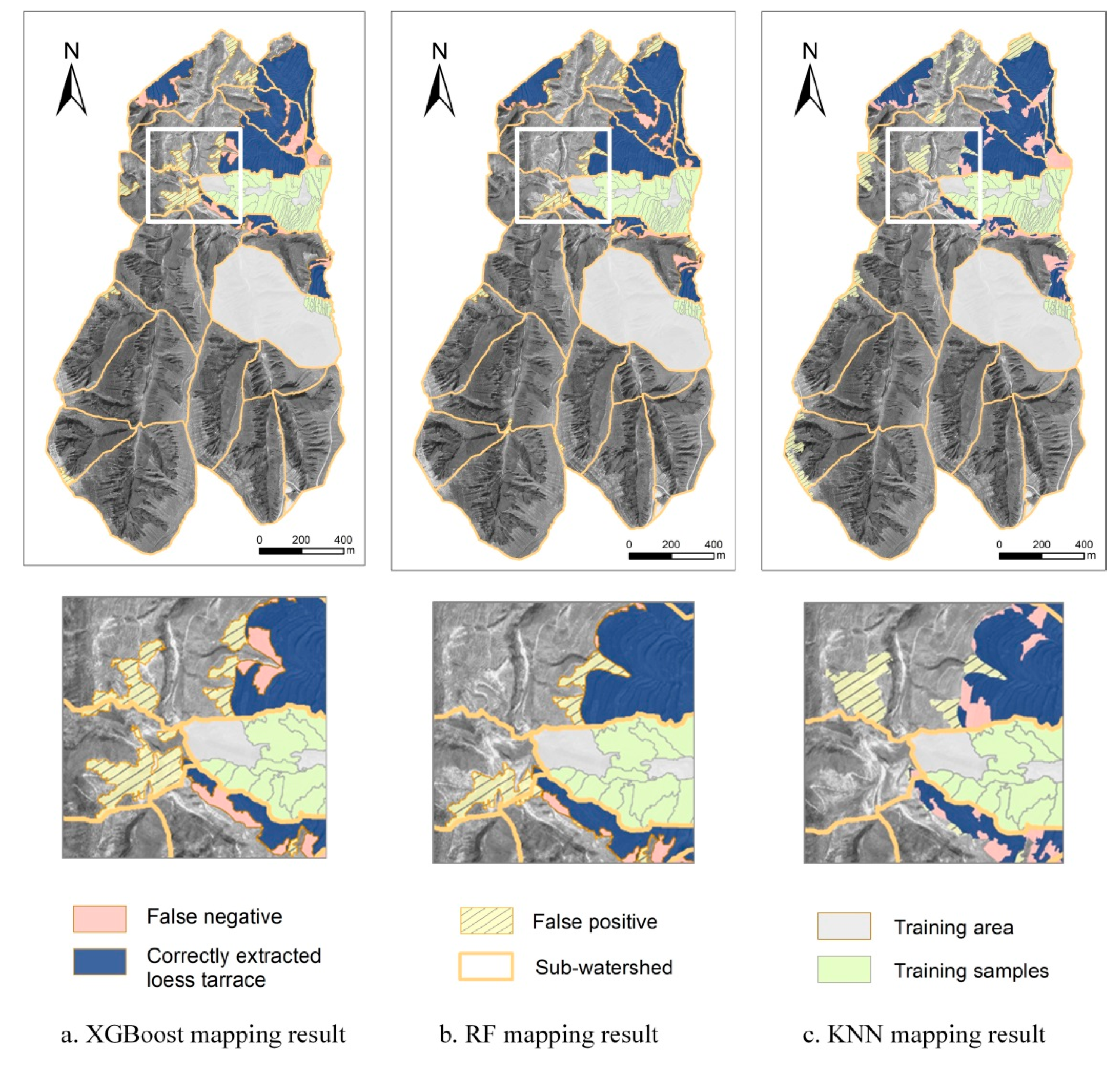
Figure 7 shows the terrace mapping results of XGBoost, RF, and KNN. The results illustrate that terraces and non-terraces were successfully detected. The results indicate that the RF classifier performed excellently by creating an accurate terrace inventory map with only limited incorrectly extracted and unextracted terraces. The visual assessment indicates that for terrace mapping, RF is more reliable than KNN or XGBoost. Most of the incorrectly detected terraces (false positives) in the study area were identified with the KNN classifier rather than RF or XGBoost. Most of the non-detected terraces (false negatives) in the study area were identified with the XGBoost classifier rather than RF or KNN.
Four types of belief measurements, namely, Pr, Re, OA, and k, were adopted to validate the mapping results in this study because of their high performance in previous studies. As previously mentioned, F1 can reflect the balance between Pr and Re. Thus, F1 was utilized to evaluate the pixel coverage for quantitatively detecting terraces. The belief masses for labeled features caused by the classifiers were calculated with a confusion matrix. Table 3 indicates the performance of three classifiers in the testing area. Among the three classifiers, RF performed best in terms of Pr, Re, and F1 with 88.15%, 83.63%, and 85.83%, respectively, followed by XGBoost classifiers with 81.96%, 81.48%, and 81.72%. The KNN classifier obtained the lowest F1 score (77.19%) because of its lower Pr (73.36%) than the others, although its recall value was good (81.44%). In accordance with the accuracy assessment result, the RF classifier achieved an OA of up to 95.60% and accurately identified the terraces among the object-based classifiers. This result was followed by XGBoost and KNN classifiers with 94.19% and 92.33%, respectively. Although the three classifiers had an OA of more than 90%, RF had the highest k value of 0.83, which is considered as approximately perfect. The accuracy assessment proved that the RF classifier was effective and may be applied to other regions that exhibit similar conditions to those in the present study.

4. Discussion

4.1. Influence of Class Imbalance and Feature Selection on Terrace Mapping

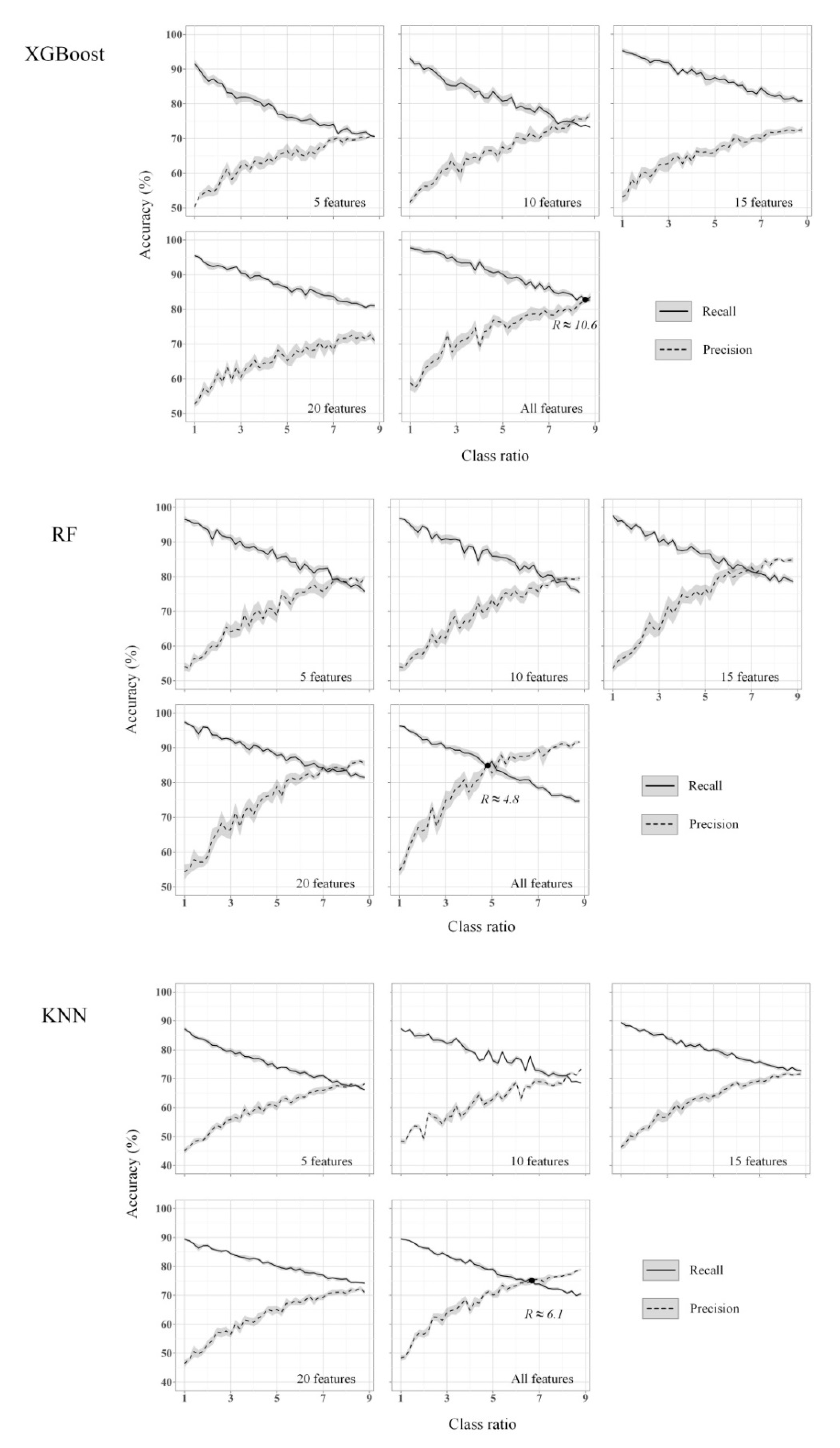
Class imbalance refers to when the total number of one class far exceeds the number of another, thereby giving rise to a low predictive accuracy for the infrequent class. The class imbalance effect needs to be considered because the covered areas of terraces are discrete and small in the study area. Previous studies demonstrated that undersampling of the majority class is a beneficial strategy to overcome the class imbalance problem [27,55,62]. To estimate the class imbalance effect, the training samples were divided into subtraining and subtesting samples. Later, a metric R was defined as the ratio of terrace and non-terrace segments in the current subtraining. Then, an iterative procedure was used to estimate a target R value for the emerging balance between Pr and Re on the subtesting samples. In each iteration, all the terrace segments and R-fold numbers of non-terrace samples were randomly sampled from the subtraining datasets to train the ML classifiers and assess the accuracies on the remaining subtesting samples. The procedure began from R = 1 and increased by 0.2 in each step. For evaluating the effect of different feature combinations on terrace mapping, five feature combinations were utilized, where the top 5, top 10, top 15, and 20 features based on Table 2 were selected, and all the 55 features were chosen.
In this study, the training area was divided into subtraining and subtesting at a ratio of 1:3 because the number of samples in the validation datasets (2596 segments) was approximately three times higher than the training samples (849 segments). Therefore, 221 segments, including 20 terrace and 183 non-terrace segments, were randomly selected as subtraining samples, and the remaining 646 segments were treated as subtesting samples. For each R, the procedure was repeated 10 times on the basis of randomly sampled subtraining and subtesting segments from training datasets based on different feature combinations. Then, the mean error rates and their standard deviations were calculated. The experimental results are shown in Figure 8.
The trends of three ML classifiers in terms of the accuracy value based on different class ratios (R) and feature combinations are similar. As shown in Figure 5, Re is approximately 100% when the value of the class balanced ratio R is set to one. However, the precision is lower than 20%, implying that the extent of terraces are overestimated. As shown in Figure 8, converging curves of the Re and Pr accuracy appear when the value of R changes from one to nine. For the RF, the converging curves can be crossed using five different feature combinations. However, for the XGBoost and KNN, this unique crossing for the converging curves can be achieved only when all the features are used, as shown in Figure 5. The highest balanced Re and Pr for RF that can be achieved was approximately 86% when R ≈ 4.8, which is significantly higher than XGBoost (approximately 81%) and KNN (approximately 75%). RF can obtain 85% Re and Pr when 20 features are applied. This circumstance may imply that training an RF model does not need large datasets.

4.2. General Discussion

Although experiments show that the RF classifier outperforms other state-of-the-art ML classifiers in terms of classification accuracy, some important considerations about its efficiency need to be further discussed. KNN has a lower efficiency as compared with ensemble classifiers because it is unsuitable for parallel processing. XGBoost and RF have a higher accuracy than KNN. The basic principle behind ensemble learning is that by combining a series of classifiers the performance is slightly better than “random guessing”, similar to KNN [51].
The comparison in this work was conducted in a hilly area characterized by severe soil erosion in the Loess Plateau, China. Although the landform in the Loess Plateau has spatial heterogeneity, the distribution pattern of loess landform has a certain regularity. Therefore, the entire OBIA-ML framework is universal, including image segmentation, feature selection, and ML classification. The results from this study area are to some extent transferable to other Loess Plateau regions.
Although ML in the OBIA framework demonstrated a good performance in artificial terrace mapping, the classification works have several limitations. Only the artificial terrace area can be identified rather than the boundaries of each individual terrace (known as terrace ridges). To improve the mapping task, other data sources, such as lidar, along with a variety of terrain attributes, can be considered. Apart from ML classifiers, deep learning (DL) has become popular. The feature selection in the numbers and choices will certainly affect the final classification accuracy. By contrast to the mandatory feature selection in ML, the features in DL are automatically learned during classifier training. These distinctive machine-learned features, such as spectral, contextual, and spatial features, will lead to the increase in their generalizability. The training process in DL is time-consuming, and an improved model network manual design is strongly required. These topics will be explored in future studies.

5. Conclusions

Artificial terraces are common around the world and are of great importance in food production, water and soil conservation, and ecologic protection. Automatic, efficient, high-accuracy mapping of artificial terraces is the basis of this field of study. OBIA has been widely applied in remote sensing image classification and essentially consists of image segmentation, feature selection, and classification. In this study, we explored the potential of an object-based ML framework for artificial terrace mapping. Three object-based ML classifiers (i.e., XGBoost, RF, and KNN) were evaluated in an artificial terrace mapping comparison. We conducted experiments on an area of the Loess Plateau, China, through 1-m resolution aerial imagery and DEM from UAV photogrammetry. The results indicate that the RF model obtains the most accurate classification results, and the KNN and XGBoost classifiers produce acceptably accurate classification results. The influence of class imbalance and feature selection was analyzed and discussed. In this study, one of our hypotheses was that the use of objective feature selection would improve the classification results.
The final conclusion drawn from this study is that the OBIA framework for artificial terrace mapping can still be improved. DL and certain other data sources, such as lidar, may help to enhance the OBIA framework. This will require several in-depth studies in the future.

Author Contributions

Conceptualization: H.D. and J.N.; methodology: H.D. and J.N.; software: H.D.; validation: H.D. and S.J.; formal analysis: H.D.; writing—original draft preparation: H.D., J.N., and S.J.; writing—review and editing: J.N., J.Z., K.L., Y.F., and F.L.; visualization: H.D.; supervision: J.N.; funding acquisition: H.D, K.L., and J.Z. All authors have read and agreed to the published version of the manuscript.

Funding

This work was financially supported by the Natural Science Foundation of China (Nos. 42001329 and 41801321), the foundation of Key Lab of Virtual Geographic Environment (Nanjing Normal University), Ministry of Education (No. 2020VGE04) and the talent research start-up funding project of Nanjing Forestry University (No. GXL2018049).

Data Availability Statement

Data from this research will be available upon request to the authors.

Conflicts of Interest

The authors declare no conflict of interest.

Appendix A

The detailed descriptions of the features used in this study for mapping terraces.
Table A1. The descriptions of the features used for mapping terraces.
TypeFeaturesDescriptions
SpectrumMean band (Red, Green, Blue, and Panchromatic band) The mean intensity of all pixels forming an image object within each band,
C ¯ = 1 n i = 1 n C i
where Ci denotes the intensity value at the pixel in an image object; and n is the total number of an object.
BrightnessThe mean value of the C of all layers,
B = 1 n L i = 1 n C i ¯ ,
where C i ¯ denotes the mean intensity value of layer i; and nL is the total number of layers.
Maximum DifferenceSpectrum difference of all layers,
M a x D i f f = m a x | C i ¯ ( k ) C j ¯ ( k ) | B ( k )
where i, j are image layers; B(v) is the brightness of the image object k; C i ¯ ( k ) is the mean intensity of image layer i of image object k; and C j ¯ ( k ) is the mean intensity of image layer j of image object k.
GeometryShape index The smoothness of an image object border,
SI = b k 4 P k ,
where bk is the border length of image object k, which is defined as the sum of the edges of the object k. Pk is the total number of pixels contained in object k. The smoother the border of an image object, the lower its shape index.
Length–widthA length-to-width ratio of an image object,
r = a 2 + [ ( 1 f ) b ] 2 P k ,
where f = P k a · b ; a and b are the length and width of the bounding box of the image object k. Pk is the total number of pixels contained in object k.
RoundnessSimilarity of an object to an ellipse,
Roundness = e k m a x e k m i n ,
where e k m a x and e k m i n are the radius of the largest and smallest enclose ellipse of image object k, respectively.
AreaThe number of pixels forming an image object.
TopographyMean value (Elevation, Curvature, Roughness, Slope, and Shaded relief)The mean intensity of all pixels forming an image object within each topographic layer.
Terrain textureGray-level co-occurrence matrix (GLCM) homogeneityThe GLCM measures how often different combinations of pixel gray levels occur in a scene. In this study, the terrain texture features were derived from GLCM based on five topographic layers. The detail for calculating GLCM was taken from the study by Haralick et al. (1973) [63].
GLCM contrast
GLCM dissimilarity
GLCM entropy
GLCM angular second moment
GLCM mean
GLCM standard deviation
GLCM correlation

References

  1. Arnáez, J.; Lana-Renault, N.; Lasanta, T.; Ruiz-Flaño, P.; Castroviejo, J. Effects of farming terraces on hydrological and geomorphological processes. A review. Catena 2015, 128, 122–134. [Google Scholar] [CrossRef] [Green Version]
  2. Fu, B. Soil erosion and its control in the Loess Plateau of China. Soil Use Manag. 1989, 5, 76–82. [Google Scholar] [CrossRef]
  3. van Wesemael, B.; Poesen, J.; Benet, A.S.; Barrionuevo, L.C.; Puigdefábregas, J. Collection and storage of runoff from hillslopes in a semi-arid environment: Geomorphic and hydrologic aspects of the aljibe system in Almeria Province, Spain. J. Arid Environ. 1998, 40, 1–14. [Google Scholar] [CrossRef] [Green Version]
  4. Sofia, G.; Roder, G.; Dalla Fontana, G.; Tarolli, P. Flood dynamics in urbanised landscapes: 100 years of climate and humans’ interaction. Sci. Rep. 2017, 7, 40527. [Google Scholar] [CrossRef] [PubMed]
  5. Arabi, M.; Frankenberger, J.R.; Engel, B.A.; Arnold, J.G. Representation of agricultural conservation practices with SWAT. Hydrol. Process. 2008, 22, 3042–3055. [Google Scholar] [CrossRef]
  6. Shi, Z.; Ai, L.; Fang, N.; Zhu, H. Modeling the impacts of integrated small watershed management on soil erosion and sediment delivery: A case study in the Three Gorges Area, China. J. Hydrol. 2012, 438, 156–167. [Google Scholar] [CrossRef]
  7. Strehmel, A.; Jewett, A.; Schuldt, R.; Schmalz, B.; Fohrer, N. Field data-based implementation of land management and terraces on the catchment scale for an eco-hydrological modelling approach in the Three Gorges Region, China. Agric. Water Manag. 2016, 175, 43–60. [Google Scholar] [CrossRef]
  8. Cucchiaro, S.; Fallu, D.J.; Zhang, H.; Walsh, K.; van Oost, K.; Brown, A.G.; Tarolli, P. Multiplatform-SfM and TLS data fusion for monitoring agricultural terraces in complex topographic and landcover conditions. Remote Sens. 2020, 12, 1946. [Google Scholar] [CrossRef]
  9. Ritsema, C.J. Introduction: Soil erosion and participatory land use planning on the Loess Plateau in China. Catena 2003, 1, 1–5. [Google Scholar] [CrossRef]
  10. Delang, C.O.; Yuan, Z. China’s Grain for Green Program; Springer: Berlin/Heidelberg, Germany, 2016. [Google Scholar]
  11. Tsunekawa, A.; Liu, G.; Yamanaka, N.; Du, S. Restoration and Development of the Degraded Loess Plateau, China; Springer: Berlin/Heidelberg, Germany, 2014. [Google Scholar]
  12. Wen, Y.; Gao, P.; Mu, X.; Zhao, G.; Sun, W. Effect of rainfall intensity on Rill erosion on terrace wall. Res. Soil Water Conserv. 2018, 25, 6–10. [Google Scholar]
  13. Dai, W.; Na, J.; Huang, N.; Hu, G.; Yang, X.; Tang, G.; Xiong, L.; Li, F. Integrated edge detection and terrain analysis for agricultural terrace delineation from remote sensing images. Int. J. Geogr. Inf. Sci. 2020, 34, 484–503. [Google Scholar] [CrossRef]
  14. Agnoletti, M.; Cargnello, G.; Gardin, L.; Santoro, A.; Bazzoffi, P.; Sansone, L.; Pezza, L.; Belfiore, N. Traditional landscape and rural development: Comparative study in three terraced areas in Northern, Central and Southern Italy to evaluate the efficacy of GAEC standard 4.4 of cross compliance. Ital. J. Agron. 2011, 6, e16. [Google Scholar] [CrossRef]
  15. Liu, X.; Yang, S.; Wang, F.; He, X.; Ma, H.; Luo, Y. Analysis on sediment yield reduced by current terrace and shrubs-herbs-arbor vegetation in the Loess Plateau. J. Hydraul. Eng. 2014, 45, 1293–1300. [Google Scholar]
  16. Dai, W.; Hu, G.; Huang, N.; Zhang, P.; Yang, X.; Tang, G. A contour-directional detection for deriving terrace ridge from open source images and digital elevation models. IEEE Access 2019, 7, 129215–129224. [Google Scholar] [CrossRef]
  17. Na, J.; Yang, X.; Fang, X.; Tang, G.; Pfeifer, N. Mapping artificial terraces from image matching point cloud in Loess Plateau of China. Int. Arch. Photogramm. Remote Sens. Spat. Inf. Sci. 2019, 42, 469–473. [Google Scholar] [CrossRef] [Green Version]
  18. Luo, L.; Li, F.; Dai, Z.; Yang, X.; Liu, W.; Fang, X. Terrace extraction based on remote sensing images and digital elevation model in the loess plateau, China. Earth Sci. Inform. 2020, 13, 433–446. [Google Scholar] [CrossRef]
  19. Na, J.; Xue, K.; Xiong, L.; Tang, G.; Ding, H.; Strobl, J.; Pfeifer, N. UAV-based terrain modeling under vegetation in the chinese Loess plateau: A deep learning and terrain correction ensemble framework. Remote Sens. 2020, 12, 3318. [Google Scholar] [CrossRef]
  20. Martínez-Casasnovas, J.A.; Ramos, M.C.; Cots-Folch, R. Influence of the EU CAP on terrain morphology and vineyard cultivation in the Priorat region of NE Spain. Land Use Policy 2010, 27, 11–21. [Google Scholar] [CrossRef]
  21. Li, Y.; Gong, J.; Wang, D.; An, L.; Li, R. Sloping farmland identification using hierarchical classification in the Xi-He region of China. Int. J. Remote Sens. 2013, 34, 545–562. [Google Scholar] [CrossRef]
  22. Zhao, H.; Fang, X.; Ding, H.; Josef, S.; Xiong, L.; Na, J.; Tang, G. Extraction of terraces on the Loess Plateau from high-resolution DEMs and imagery utilizing object-based image analysis. ISPRS Int. J. Geo Inf. 2017, 6, 157. [Google Scholar] [CrossRef] [Green Version]
  23. Blaschke, T. Object based image analysis for remote sensing. ISPRS J. Photogramm. Remote Sens. 2010, 65, 2–16. [Google Scholar] [CrossRef] [Green Version]
  24. Drǎguţ, L.; Tiede, D.; Levick, S.R. ESP: A tool to estimate scale parameter for multiresolution image segmentation of remotely sensed data. Int. J. Geogr. Inf. Sci. 2010, 24, 859–871. [Google Scholar] [CrossRef]
  25. Ding, H.; Liu, K.; Chen, X.; Xiong, L.; Tang, G.; Qiu, F.; Strobl, J. Optimized Segmentation Based on the Weighted Aggregation Method for Loess Bank Gully Mapping. Remote Sens. 2020, 12, 793. [Google Scholar] [CrossRef] [Green Version]
  26. D’Oleire-Oltmanns, S.; Marzolff, I.; Tiede, D.; Blaschke, T. Detection of gully-affected areas by applying object-based image analysis (OBIA) in the region of Taroudannt, Morocco. Remote Sens. 2014, 6, 8287–8309. [Google Scholar] [CrossRef] [Green Version]
  27. Liu, K.; Ding, H.; Tang, G.; Zhu, A.-X.; Yang, X.; Jiang, S.; Cao, J. An object-based approach for two-level gully feature mapping using high-resolution DEM and imagery: A case study on hilly loess plateau region, China. Chin. Geogr. Sci. 2017, 27, 415–430. [Google Scholar] [CrossRef]
  28. Xiong, Z.; Zhang, X.; Wang, X.; Yuan, J. Self-adaptive segmentation of satellite images based on a weighted aggregation approach. GISci. Remote Sens. 2019, 56, 233–255. [Google Scholar] [CrossRef]
  29. Jozdani, S.E.; Momeni, M.; Johnson, B.A.; Sattari, M. A regression modelling approach for optimizing segmentation scale parameters to extract buildings of different sizes. Int. J. Remote Sens. 2018, 39, 684–703. [Google Scholar] [CrossRef]
  30. Ma, L.; Li, M.; Ma, X.; Cheng, L.; Du, P.; Liu, Y. A review of supervised object-based land-cover image classification. ISPRS J. Photogramm. Remote Sens. 2017, 130, 277–293. [Google Scholar] [CrossRef]
  31. Ma, L.; Cheng, L.; Li, M.; Liu, Y.; Ma, X. Training set size, scale, and features in Geographic Object-Based Image Analysis of very high resolution unmanned aerial vehicle imagery. ISPRS J. Photogramm. Remote Sens. 2015, 102, 14–27. [Google Scholar] [CrossRef]
  32. Hong, H.; Liu, J.; Bui, D.T.; Pradhan, B.; Acharya, T.D.; Pham, B.T.; Zhu, A.-X.; Chen, W.; Ahmad, B.B. Landslide susceptibility mapping using J48 Decision Tree with AdaBoost, Bagging and Rotation Forest ensembles in the Guangchang area (China). Catena 2018, 163, 399–413. [Google Scholar] [CrossRef]
  33. Tavakkoli Piralilou, S.; Shahabi, H.; Jarihani, B.; Ghorbanzadeh, O.; Blaschke, T.; Gholamnia, K.; Meena, S.R.; Aryal, J. Landslide detection using multi-scale image segmentation and different machine learning models in the higher himalayas. Remote Sens. 2019, 11, 2575. [Google Scholar] [CrossRef] [Green Version]
  34. Wang, Y.; Fang, Z.; Wang, M.; Peng, L.; Hong, H. Comparative study of landslide susceptibility mapping with different recurrent neural networks. Comput. Geosci. 2020, 138, 104445. [Google Scholar] [CrossRef]
  35. Zhou, D.; Zhao, S.; Zhu, C. The Grain for Green Project induced land cover change in the Loess Plateau: A case study with Ansai County, Shanxi Province, China. Ecol. Indic. 2012, 23, 88–94. [Google Scholar] [CrossRef]
  36. Li, Z.; Zhang, Y.; Zhu, Q.; He, Y.; Yao, W. Assessment of bank gully development and vegetation coverage on the Chinese Loess Plateau. Geomorphology 2015, 228, 462–469. [Google Scholar] [CrossRef]
  37. Chen, Y.; Jiao, J.; Wei, Y.; Zhao, H.; Yu, W.; Cao, B.; Xu, H.; Yan, F.; Wu, D.; Li, H. Accuracy Assessment of the Planar Morphology of Valley Bank Gullies Extracted with High Resolution Remote Sensing Imagery on the Loess Plateau, China. Int. J. Environ. Res. Public Health 2019, 16, 369. [Google Scholar] [CrossRef] [Green Version]
  38. Sharon, E.; Brandt, A.; Basri, R. Fast Multiscale Image Segmentation. In Proceedings of the IEEE Conference on Computer Vision and Pattern Recognition, CVPR 2000 (Cat. No. PR00662), Hilton Head, SC, USA, 13–15 June 2000; pp. 70–77. [Google Scholar]
  39. Sharon, E.; Brandt, A.; Basri, R. Segmentation and Boundary Detection using Multiscale Intensity Measurements. In Proceedings of the 2001 IEEE Computer Society Conference on Computer Vision and Pattern Recognition. CVPR 2001, Kauai, HI, USA, 8–14 December 2001; p. 1. [Google Scholar]
  40. Sharon, E.; Galun, M.; Sharon, D.; Basri, R.; Brandt, A. Hierarchy and adaptivity in segmenting visual scenes. Nature 2006, 442, 810–813. [Google Scholar] [CrossRef] [PubMed]
  41. Johnson, B.; Xie, Z. Unsupervised image segmentation evaluation and refinement using a multi-scale approach. ISPRS J. Photogramm. Remote Sens. 2011, 66, 473–483. [Google Scholar] [CrossRef]
  42. Xiong, L.-Y.; Zhu, A.-X.; Zhang, L.; Tang, G.-A. Drainage basin object-based method for regional-scale landform classification: A case study of loess area in China. Phys. Geogr. 2018, 39, 523–541. [Google Scholar] [CrossRef]
  43. Georganos, S.; Grippa, T.; Lennert, M.; Vanhuysse, S.; Johnson, B.A.; Wolff, E. Scale matters: Spatially partitioned unsupervised segmentation parameter optimization for large and heterogeneous satellite images. Remote Sens. 2018, 10, 1440. [Google Scholar] [CrossRef] [Green Version]
  44. Johnson, B.A.; Bragais, M.; Endo, I.; Magcale-Macandog, D.B.; Macandog, P.B.M. Image segmentation parameter optimization considering within-and between-segment heterogeneity at multiple scale levels: Test case for mapping residential areas using landsat imagery. ISPRS Int. J. Geo Inf. 2015, 4, 2292–2305. [Google Scholar] [CrossRef] [Green Version]
  45. Gómez-Gutiérrez, Á.; Conoscenti, C.; Angileri, S.E.; Rotigliano, E.; Schnabel, S. Using topographical attributes to evaluate gully erosion proneness (susceptibility) in two mediterranean basins: Advantages and limitations. Nat. Hazards 2015, 79, 291–314. [Google Scholar] [CrossRef]
  46. Belgiu, M.; Drăguţ, L. Random forest in remote sensing: A review of applications and future directions. ISPRS J. Photogramm. Remote Sens. 2016, 114, 24–31. [Google Scholar] [CrossRef]
  47. Haralick, R.M. Statistical and structural approaches to texture. Proc. IEEE 1979, 67, 786–804. [Google Scholar] [CrossRef]
  48. Yu, L.; Liu, H. Feature Selection for High-Dimensional Data: A Fast Correlation-Based Filter Solution. In Proceedings of the 20th International Conference on Machine Learning (ICML-03), Washington, DC, USA, 21–24 August 2003; pp. 856–863. [Google Scholar]
  49. Georganos, S.; Grippa, T.; Vanhuysse, S.; Lennert, M.; Shimoni, M.; Kalogirou, S.; Wolff, E. Less is more: Optimizing classification performance through feature selection in a very-high-resolution remote sensing object-based urban application. GISci. Remote Sens. 2018, 55, 221–242. [Google Scholar] [CrossRef]
  50. Chen, T.; Guestrin, C. XGBoost: Reliable Large-Scale Tree Boosting System. 2017. Available online: http://learningsys.org/papers/LearningSys_2015_paper_32.pdf (accessed on 9 October 2019).
  51. Jozdani, S.E.; Johnson, B.A.; Chen, D. Comparing deep neural networks, ensemble classifiers, and support vector machine algorithms for object-based urban land use/land cover classification. Remote Sens. 2019, 11, 1713. [Google Scholar] [CrossRef] [Green Version]
  52. Mustapha, I.B.; Saeed, F. Bioactive Molecule Prediction Using Extreme Gradient Boosting. Molecules 2016, 21, 983. [Google Scholar] [CrossRef] [PubMed] [Green Version]
  53. Xgboost: Extreme Gradient Boosting. 2016. Available online: https://mran.microsoft.com/web/packages/xgboost/vignettes/xgboost.pdf (accessed on 8 March 2021).
  54. Breiman, L. Random forests. Mach. Learn. 2001, 45, 5–32. [Google Scholar] [CrossRef] [Green Version]
  55. Stumpf, A.; Kerle, N. Object-oriented mapping of landslides using Random Forests. Remote Sens. Environ. 2011, 115, 2564–2577. [Google Scholar] [CrossRef]
  56. Shafer, G. A Mathematical Theory of Evidence; Princeton University Press: Princeton, NJ, USA, 1976; Volume 42. [Google Scholar]
  57. Bobkowska, K. Analysis of the objects images on the sea using Dempster-Shafer Theory. In Proceedings of the 2016 17th International Radar Symposium (IRS), Krakow, Poland, 10–12 May 2016; pp. 1–4. [Google Scholar]
  58. Foley, B.G. A Dempster-Shafer Method for Multi-Sensor Fusion. Master’s Thesis, Air Force Institute of Technology, Wright-Patterson AFB, OH, USA, 2012. [Google Scholar]
  59. Mezaal, M.R.; Pradhan, B.; Rizeei, H.M. Improving landslide detection from airborne laser scanning data using optimized Dempster—Shafer. Remote Sens. 2018, 10, 1029. [Google Scholar] [CrossRef] [Green Version]
  60. Ghorbanzadeh, O.; Blaschke, T.; Gholamnia, K.; Meena, S.R.; Tiede, D.; Aryal, J. Evaluation of different machine learning methods and deep-learning convolutional neural networks for landslide detection. Remote Sens. 2019, 11, 196. [Google Scholar] [CrossRef] [Green Version]
  61. Ding, H.; Na, J.-M.; Huang, X.-l.; Tang, G.-A.; Liu, K. Stability analysis unit and spatial distribution pattern of the terrain texture in the northern Shaanxi Loess Plateau. J. Mt. Sci. 2018, 15, 577–589. [Google Scholar] [CrossRef]
  62. Shruthi, R.B.; Kerle, N.; Jetten, V. Object-based gully feature extraction using high spatial resolution imagery. Geomorphology 2011, 134, 260–268. [Google Scholar] [CrossRef]
  63. Haralick, R.M.; Shanmugam, K.; Dinstein, I.H. Textural features for image classification. IEEE Trans. Syst. Man Cybern. 1973, SMC-3, 610–621. [Google Scholar] [CrossRef] [Green Version]
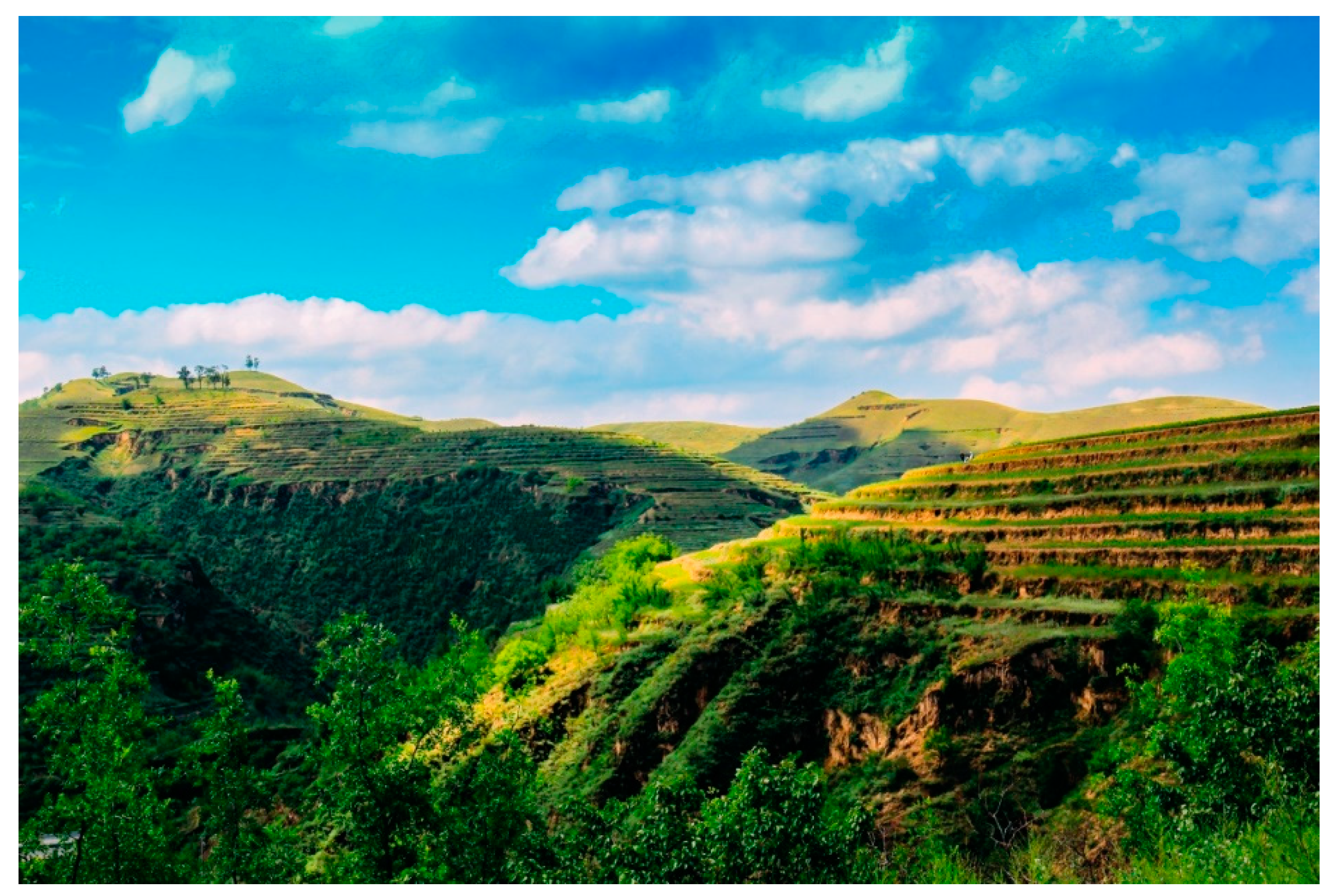
Figure 1. Artificial terraces in Ansai, the Loess Plateau, China, which have almost returned to grassland after the implement of “Grain for Green” project. Erosion can be observed between the ridges of the terraces due to the lack of maintenance.
Remotesensing 13 01021 g001
Figure 2. Study area and data. (a,b) show the location of the Loess Plateau, China, and the study area. (c) Digital elevation models (DEMs) of the study area, and (d) WorldView-3 imagery of the study area with ground truth.
Remotesensing 13 01021 g002
Figure 3. Details of terraces in the study area. (a) Ortho-image of a subset (white polygon) in the study area; (bf) show the panchromatic band, elevation, slope, shaded relief, and curvature of the subset, respectively.
Remotesensing 13 01021 g003
Figure 4. Workflow of the proposed method.
Remotesensing 13 01021 g004
Figure 5. Examples of selected features for terrace mapping.
Remotesensing 13 01021 g005
Figure 6. Segmentation result and training samples.
Remotesensing 13 01021 g006
Figure 7. Mapping results based on three machine learning (ML) classifiers.
Remotesensing 13 01021 g007
Figure 8. Estimates of the class ratio (R) in the training stage that triggers a balance of Table 10. fold random replicate runs. The gray margins represent the corresponding standard deviations.
Remotesensing 13 01021 g008
Table 1. Overview of the features used for mapping terraces.
TypeFeatures
SpectrumMean band (Red, Green, Blue, and Panchromatic band), Maximum Difference, and Brightness
GeometryShape index, Length–width, Roundness, and Area
TopographyMean value (Elevation, Curvature, Roughness, Slope, and Shaded relief)
Terrain textureGray-level co-occurrence matrix (GLCM) homogeneity, GLCM contrast, GLCM dissimilarity, GLCM entropy, GLCM angular second moment, GLCM mean, GLCM standard deviation, and GLCM correlation based on Elevation, Curvature, Roughness, Slope, and Shaded relief
Table 2. Feature selection result using the correlation-based feature selection (CFS) method.
Feature TypeFeatureIterationAverage Rank
SpectrumMean value of panchromatic band201.0
Terrain textureGLCM angular second moment of curvature202.4
Terrain textureGLCM homogeneity of shade relief205.0
Terrain textureGLCM homogeneity of curvature205.9
SpectrumMaximum difference of value207.0
SpectrumMean value of band red 207.1
Terrain textureGLCM mean value of shade relief207.1
GeometryLength/Width207.3
Terrain textureGLCM angular second moment of elevation209.8
Terrain textureGLCM homogeneity of slope2010.4
TopographyMean value of shade relief2010.9
Terrain textureGLCM angular second moment of shade relief2012.0
Terrain textureGLCM mean value of roughness2012.4
Terrain textureGLCM homogeneity of roughness1913.0
Terrain textureGLCM standard derivation of curvature 1814.1
SpectrumMean value of band green 1619.0
Terrain textureGLCM mean value of slope1119.7
GeometryArea1220.5
TopographyMean value of elevation820.9
GeometryShape index522.1
Table 3. Accuracy assessment (confusion matrix) on the study area.
ClassifierMapping ResultsReference (m2)PrReF1OAKappa
TerracesNon-Terraces
XGBoostTerraces222,855.5549,058.7881.96%81.48%81.72%94.19%0.78
Non-Terraces50,638.181,393,215.99
RFTerraces228,722.8130,747.1988.15%83.63%85.83%95.60%0.83
Non-Terraces44,770.921,411,527.58
KNNTerraces222,743.5980,880.6573.36%81.44%77.19%92.33%0.73
Non-Terraces50,750.141,361,394.12
Publisher’s Note: MDPI stays neutral with regard to jurisdictional claims in published maps and institutional affiliations.