Modeling and Analysis of BDS-2 and BDS-3 Combined Precise Time and Frequency Transfer Considering Stochastic Models of Inter-System Bias

Abstract

BeiDou global navigation satellite system (BDS) began to provide positioning, navigation, and timing (PNT) services to global users officially on 31 July, 2020. BDS constellations consist of regional (BDS-2) and global navigation satellites (BDS-3). Due to the difference of modulations and characteristics for the BDS-2 and BDS-3 default civil service signals (B1I/B3I) and the increase of new signals (B1C/B2a) for BDS-3, a systemically bias exists in the receiver-end when receiving and processing BDS-2 and BDS-3 signals, which leads to the inter-system bias (ISB) between BDS-2 and BDS-3 on the receiver side. To fully utilize BDS, the BDS-2 and BDS-3 combined precise time and frequency transfer are investigated considering the effect of the ISB. Four kinds of ISB stochastic models are presented, which are ignoring ISB (ISB_NO), estimating ISB as random constant (ISB_CV), random walk process (ISB_RW), and white noise process (ISB_WN). The results demonstrate that the datum of receiver clock offsets can be unified and the ISB deduced datum confusion can be avoided by estimating the ISB. The ISB_CV and ISB_RW models are superior to ISB_WN. For the BDS-2 and BDS-3 combined precise time and frequency transfer using ISB_NO, ISB_CV, ISB_RW, and ISB_WN, the stability of clock differences of old signals can be enhanced by 20.18%, 23.89%, 23.96%, and 11.46% over BDS-2-only, respectively. For new signals, the enhancements are −50.77%, 20.22%, 17.53%, and −3.69%, respectively. Moreover, ISB_CV and ISB_RW models have the better frequency transfer stability. Consequently, we recommended the optimal ISB_CV or suboptimal ISB_RW model for BDS-2 and BDS-3 combined precise time and frequency transfer when processing the old as well as the new signals.

1. Introduction

As the third navigation satellite system recognized by International Maritime Organization (IMO), the development and construction of BeiDou navigation satellite system (BDS) has experienced three stages: The demonstration system (BDS-1), the regional system (BDS-2), and then the global system (BDS-3) [1,2,3]. BDS-2 contains five geostationary earth orbit (GEO), seven inclined geosynchronous satellite orbit (IGSO), and three medium earth orbit (MEO) satellites, which can transmit three frequency signals i.e., B1I (1561.098 MHz), B2I (1207.14 MHz), and B3I (1268.52 MHz) [4]. The new-generation BDS-3 consists of 3 GEO, 24 MEO, and 3 IGSO satellites, which can transmit more frequency signals including the new signals B1C (1575.42 MHz), B2a (1176.45 MHz), and B2b (1207.14 MHz) as well as the old signals B1I and B3I [1]. With the rapid development and construction of BDS, BDS officially began to provide global positioning, navigation, and timing (PNT) services on 31 July 2020.

The time of the fourth dimension is of great interest in the Global Navigation Satellite System (GNSS) community. In the time community, the common view (CV) and all-in view (AV) techniques are utilized for GNSS time and frequency transfer [5,6,7]. The CV technique, by observing the same satellites to remove the common satellites errors, can achieve 1 to 10 ns accuracy of time transfer [8]. Due to the limitation of the baseline length, the CV technique is difficult to realize global time transfer. Unlike CV technique, the AV technique can get rid of the limitation of the baseline length and achieve global time transfer [6]. Thanks to the development of precise orbit and clock products in terms of precision and timeliness, precise point positioning (PPP) as a typical AV technique is of great interest in the time and frequency field, which can obtain the sub-nanosecond to nanosecond accuracy [9]. With the development of International GNSS Service (IGS) Multi-GNSS Experiment (MGEX), multi-GNSS PPP time and frequency transfer becomes a hot topic, Defraigne and Baire [10] investigated the GPS, GPS/GLONASS combined time and frequency transfer, showing that the stability can be improved by adding the GLONASS observations. Ge, et al. [11] compared GPS, BDS-2, Galileo, and multi-GNSS (GPS/BDS-2/GLONASS/Galileo) time and frequency transfer, indicating that the stability of multi-GNSS time and frequency transfer is 20.3%, 84%, and 45.4% higher than that of GPS, BDS-2, and Galileo solutions, respectively. Furthermore, Zhang, et al. [12] got similar conclusions. As for BDS PPP time and frequency transfer, Tu, et al. [13] indicated that the BDS-2 triple-frequency un-combined PPP model can be applied for precise time and frequency transfer, whose accuracy and stability were the same as the dual-frequency ionospheric-free (IF) PPP model. Su and Jin [14] demonstrated BDS-2 and BDS-3 combined time and frequency transfer by using a triple-frequency PPP model, indicating that the stability of 10,000 s for BDS time and frequency transfer is better than $1.5\times {10}^{-14}$. However, the assessment and analysis of precise time and frequency transfer using BDS-3 observations were still lacking, especially for new signals (B1C/B2a).

In terms of multi-GNSS combined data processing, the hardware delay bias between different satellite systems is a critical factor, which affects the accuracy of positioning and the stability of time and frequency transfer [15,16]. Actually, the BDS-2 and BDS-3 are two generation navigation satellite systems, their corresponding signal modulations and characteristics have both changed as shown in

Table 1. The properties of the selected stations.

System	Signal	Signal Component	Carrier Frequency (MHz)	Modulation	Chip Rate (Mcps)
BDS-2	B1I	-	1561.098	Quadrature phase-shift keying (QPSK)	2.046
	B2I	-	1207.140	QPSK	2.046
	B3I	-	1268.520	Binary phase-shift keying (BPSK)	10.23
BDS-3	B1I	-	1561.098	BPSK	2.046
	B1C	B1C_data	1575.420	Binary offset carrier (BOC)	1.023
		B1C_pilot		Quadrature Multiplexed Binary Offset Carrier (QMBOC)
	B2a	-	1176.450	BPSK	10.23
	B2b	-	1207.140	BPSK	10.23
	B3I	-	1268.520	BPSK	10.23

[17,18,19,20]. Comparing the B1I signal of BDS-2 and BDS-3, the signal modulation has changed. It is worth mentioning that BDS-3 adds new signals of B1C (1575.42 MHz), B2a (1176.45 MHz), and B2b (1207.14 MHz) besides the original signals of B1I (1561.098 MHz) and B3I (1268.52 MHz) [1,20]. Due to the increase of new signals and the change of signal modulation, some receiver manufacturers added a new signal receiving and processing unit to receive and handle the BDS-3 signals based on BDS-2 original receiver, others changed the signal processing algorithms to receive and handle the BDS-3 signals, which causes the hardware units or the signal processing algorithms of BDS-2 and BDS-3 to be inconsistent [21,22]. This inconsistency of the hardware units or the signal processing algorithms results in the difference of time delay between BDS-2 and BDS-3 on receiver side. Therefore, there is an inter-system bias (ISB) between BDS-2 and BDS-3 on receiver side. However, the current existing research on BDS-2 and BDS-3 combined time and frequency transfer basically ignore the effect of ISB on precise time and frequency transfer. Only Qin, et al. [23] performed the BDS-2 and BDS-3 combined time and frequency transfer by estimating ISB for the old signals (B1I/B3I) and indicated that estimating ISB as random constant (ISB_CV) and random walk process (ISB_RW) are potentially the better approaches, but the ISB for the new signals (B1C/B2a) were not investigated. The ISB will destroy the datum of receiver clock offsets and bias the receiver clock offsets between BDS-2 and BDS-3. To take advantage of the BDS performance, developing the technology of BDS-2 and BDS-3 combined PNT is very meaningful, especially for the research of BDS-3 new signals (B1C/B2a). Furthermore, the accuracy and the datum of precise orbit and clock products will inevitably affect the ISB estimates, and the experimental conclusions drawn by the precise satellite products obtained by a single analysis center (AC) lack slight universality and reliability.

With this background, we research the characteristic of ISB between BDS-2 and BDS-3 for both new signals (B1C/B2a) and old signals (B1I/B3I) based on precise satellite products provided by Wuhan University (WHU) and Helmholtz Centre Potsdam German Research Center for Geosciences (GFZ). We present four kinds of ISB stochastic models called ignoring ISB (ISB_NO), ISB_CV, ISB_RW, and ISB_WN to explore the influence of ISB on BDS-2 and BDS-3 combined precise time and frequency transfer. First, we present the mathematical model of BDS-2 and BDS-3 combined precise time and frequency transfer and the stochastic models of ISB in Section 2. Especially for the new signals (B1C/B2a), the detailed formulas are developed. Then, the data processing strategies of BDS-2 and BDS-3 combined precise time and frequency transfer with the selected observation data provided by IGS MGEX and international GNSS Monitoring and Assessment System (iGMAS) are shown in Section 3. In the following section, we research the characteristic of ISB for both new signals (B1C/B2a) and old signals (B1I/B3I) including the stability, rate, and its impact on ambiguity and residuals. Furthermore, the impact of different ISB stochastic models on performances of the combined precise time and frequency transfer are validated based on different time-links established by the experimental datasets. Finally, some conclusions and recommendations are given.

2. Methods

This section begins with the single frequency PPP models for BDS. Then, the BDS-2 and BDS-3 combined PPP model for both the new signals (B1C/B2a) and old signals (B1I/B3I) are introduced in detail. For the processing methods of the ISB between BDS-2 and BDS-3, four kinds of ISB stochastic models called ISB_NO, ISB_CV, ISB_RW, and ISB_WN are presented.

2.1. BDS-2 and BDS-3 Combined PPP Model

The dual-frequency IF PPP models are used to perform precise time and frequency transfer. The IF PPP models can be derived from single frequency PPP model. The single frequency PPP model for BDS can be expressed as:

$$\{\begin{array}{l}{\mathrm{P}}_{\mathrm{r},\mathrm{j}}^{\mathrm{s}}={\mathrm{u}}_{\mathrm{r}}^{\mathrm{s}}\cdot \mathrm{x}+\mathrm{c}\cdot \left(\mathsf{\delta }{\mathrm{t}}_{\mathrm{r}}+{\mathrm{b}}_{\mathrm{r},\mathrm{j}}\right)-\mathrm{c}\cdot \left(\mathsf{\delta }{\mathrm{t}}^{\mathrm{s}}+{\mathrm{b}}_{\mathrm{j}}^{\mathrm{s}}\right)+{\mathrm{g}}_{\mathrm{W}}\cdot {\mathsf{\tau }}_{\mathrm{W}}+{\mathrm{I}}_{\mathrm{r},\mathrm{j}}^{\mathrm{s}}+{\mathsf{\epsilon }}_{{\mathrm{P}}_{\mathrm{j}}}\\ {\mathrm{\Phi }}_{\mathrm{r},\mathrm{j}}^{\mathrm{s}}={\mathrm{u}}_{\mathrm{r}}^{\mathrm{s}}\cdot \mathrm{x}+\mathrm{c}\cdot \left(\mathsf{\delta }{\mathrm{t}}_{\mathrm{r}}+{\mathrm{B}}_{\mathrm{r},\mathrm{j}}\right)-\mathrm{c}\cdot \left(\mathsf{\delta }{\mathrm{t}}^{\mathrm{s}}+{\mathrm{B}}_{\mathrm{j}}^{\mathrm{s}}\right)+{\mathrm{g}}_{\mathrm{W}}\cdot {\mathsf{\tau }}_{\mathrm{W}}-{\mathrm{I}}_{\mathrm{r},\mathrm{j}}^{\mathrm{s}}+{\mathsf{\lambda }}_{\mathrm{j}}\cdot {\mathrm{N}}_{\mathrm{r},\mathrm{j}}^{\mathrm{s}}+{\mathsf{\epsilon }}_{{\mathrm{\Phi }}_{\mathrm{j}}}\end{array}$$

(1)

where P and $\mathrm{\Phi }$ are the observed-minus-computed pseudorange and carrier phase observations, respectively; s, r and j (j = 1, 2, 3, 4) refer to BDS satellite, receiver, and the BDS frequency band (B1I, B3I, B1C and B2a); ${\mathrm{u}}_{\mathrm{r}}^{\mathrm{s}}$ denotes the unit vector; x represents the receiver position increments in three directions; $\mathsf{\delta }{\mathrm{t}}_{\mathrm{r}}$ and $\mathsf{\delta }{\mathrm{t}}^{\mathrm{s}}$ represent the receiver and satellite clock offsets, respectively; ${\mathrm{b}}_{\mathrm{r},\mathrm{j}}$ and ${\mathrm{B}}_{\mathrm{r},\mathrm{j}}$ denote the frequency-dependent receiver uncalibrated code delays (UCDs) and uncalibrated phase delays (UPDs); ${\mathrm{b}}_{\mathrm{j}}^{\mathrm{s}}$ and ${\mathrm{B}}_{\mathrm{j}}^{\mathrm{s}}$ denote the frequency-dependent satellite UCDs and UPDs; ${\mathsf{\tau }}_{\mathrm{W}}$ is the zenith wet delay (ZWD) with its wet mapping function ${\mathrm{g}}_{\mathrm{W}}$; ${\mathrm{I}}_{\mathrm{r},\mathrm{j}}^{\mathrm{s}}$ is the slant ionospheric delay on the jth frequency; ${\mathsf{\lambda }}_{\mathrm{j}}$ and ${\mathrm{N}}_{\mathrm{j}}$ are the wavelength of jth frequency and the corresponding integer ambiguity; ${\mathsf{\epsilon }}_{{\mathrm{P}}_{\mathrm{j}}}$ and ${\mathsf{\epsilon }}_{{\mathsf{\Phi }}_{\mathrm{j}}}$ are the pseudo-range and carrier phase observation noises containing higher-order ionospheric delay and multipath.

Traditionally, the IF observables are used to calculate the final precise satellite clock products [24]. Therefore, the satellite UCDs of IF combination will be absorbed by the estimated satellite clock. The B1I and B3I are used to perform BDS precise orbit determination (POD) and precise clock estimation (PCE) for WHU and GFZ [25,26,27,28,29], which can be expressed as:

$$\mathsf{\delta }{\mathrm{t}}_{\mathrm{I}\mathrm{F}}^{\mathrm{s}}=\mathsf{\delta }{\mathrm{t}}^{\mathrm{s}}+\left({\mathsf{\alpha }}_{1,2}\cdot {\mathrm{b}}_1^{\mathrm{s}}+{\mathsf{\beta }}_{1,2}\cdot {\mathrm{b}}_2^{\mathrm{s}}\right)+\mathrm{d}\mathrm{D}=\mathsf{\delta }{\mathrm{t}}^{\mathrm{s}}+{\mathrm{b}}_{{}_{\mathrm{I}{\mathrm{F}}_{1,2}}}^{\mathrm{s}}+\mathrm{d}\mathrm{D}$$

(2)

where ${\mathsf{\delta }\mathrm{t}}_{\mathrm{IF}}^{\mathrm{s}}$ is the precise satellite clock offsets; dD is the bias determined by clock datum introduced through precise satellite clock estimation and universal for all satellites of one navigation system [30].

To eliminate the effect of satellite UCDs on BDS PPP, the corresponding corrections need to be considered, which read.

$$\{\begin{array}{l}{\overline{\mathrm{P}}}_{\mathrm{r},1}^{\mathrm{s}}={\mathrm{P}}_{\mathrm{r},1}^{\mathrm{s}}-\mathrm{c}\cdot \left[\frac{{\mathrm{f}}_2^2}{{\mathrm{f}}_1^2-{\mathrm{f}}_2^2}\left({\mathrm{b}}_1^{\mathrm{s}}-{\mathrm{b}}_2^{\mathrm{s}}\right)\right]\\ {\overline{\mathrm{P}}}_{\mathrm{r},2}^{\mathrm{s}}={\mathrm{P}}_{\mathrm{r},2}^{\mathrm{s}}-\mathrm{c}\cdot \left[\frac{{\mathrm{f}}_1^2}{{\mathrm{f}}_1^2-{\mathrm{f}}_2^2}\left({\mathrm{b}}_1^{\mathrm{s}}-{\mathrm{b}}_2^{\mathrm{s}}\right)\right]\\ {\overline{\mathrm{P}}}_{\mathrm{r},3}^{\mathrm{s}}={\mathrm{P}}_{\mathrm{r},3}^{\mathrm{s}}-\mathrm{c}\cdot \left[\frac{{\mathrm{f}}_2^2}{{\mathrm{f}}_1^2-{\mathrm{f}}_2^2}\left({\mathrm{b}}_1^{\mathrm{s}}-{\mathrm{b}}_2^{\mathrm{s}}\right)-\left({\mathrm{b}}_1^{\mathrm{s}}-{\mathrm{b}}_3^{\mathrm{s}}\right)\right]\\ {\overline{\mathrm{P}}}_{\mathrm{r},4}^{\mathrm{s}}={\mathrm{P}}_{\mathrm{r},4}^{\mathrm{s}}-\mathrm{c}\cdot \left[\frac{{\mathrm{f}}_2^2}{{\mathrm{f}}_1^2-{\mathrm{f}}_2^2}\left({\mathrm{b}}_1^{\mathrm{s}}-{\mathrm{b}}_2^{\mathrm{s}}\right)-\left({\mathrm{b}}_1^{\mathrm{s}}-{\mathrm{b}}_4^{\mathrm{s}}\right)\right]\end{array}$$

(3)

For IF combination, it can be expressed as:

$$\{\begin{array}{l}{\mathsf{\alpha }}_{\mathrm{m},\mathrm{n}}=\frac{{\mathrm{f}}_{\mathrm{m}}^2}{{\mathrm{f}}_{\mathrm{m}}^2-{\mathrm{f}}_{\mathrm{n}}^2},{\mathsf{\beta }}_{\mathrm{m},\mathrm{n}}=\frac{-{\mathrm{f}}_{\mathrm{n}}^2}{{\mathrm{f}}_{\mathrm{m}}^2-{\mathrm{f}}_{\mathrm{n}}^2}\\ {\mathrm{P}}_{\mathrm{r},\mathrm{I}{\mathrm{F}}_{\mathrm{m},\mathrm{n}}}^{\mathrm{s}}={\mathsf{\alpha }}_{\mathrm{m},\mathrm{n}}\cdot {\mathrm{P}}_{\mathrm{m}}^{\mathrm{s}}+{\mathsf{\beta }}_{\mathrm{m},\mathrm{n}}\cdot {\mathrm{P}}_{\mathrm{n}}^{\mathrm{s}},{\mathsf{\Phi }}_{\mathrm{r},\mathrm{I}{\mathrm{F}}_{\mathrm{m},\mathrm{n}}}^{\mathrm{s}}={\mathsf{\alpha }}_{\mathrm{m},\mathrm{n}}\cdot {\mathsf{\Phi }}_{\mathrm{m}}^{\mathrm{s}}+{\mathsf{\beta }}_{\mathrm{m},\mathrm{n}}\cdot {\mathsf{\Phi }}_{\mathrm{n}}^{\mathrm{s}}\\ {\mathrm{b}}_{\mathrm{I}{\mathrm{F}}_{\mathrm{m},\mathrm{n}}}^{\mathrm{s}}={\mathsf{\alpha }}_{\mathrm{m},\mathrm{n}}\cdot {\mathrm{b}}_{\mathrm{m}}^{\mathrm{s}}+{\mathsf{\beta }}_{\mathrm{m},\mathrm{n}}\cdot {\mathrm{b}}_{\mathrm{n}}^{\mathrm{s}},{\mathrm{b}}_{\mathrm{r},\mathrm{I}{\mathrm{F}}_{\mathrm{m},\mathrm{n}}}={\mathsf{\alpha }}_{\mathrm{m},\mathrm{n}}\cdot {\mathrm{b}}_{\mathrm{r},\mathrm{m}}+{\mathsf{\beta }}_{\mathrm{m},\mathrm{n}}\cdot {\mathrm{b}}_{\mathrm{r},\mathrm{n}}\\ {\mathrm{B}}_{\mathrm{I}{\mathrm{F}}_{\mathrm{m},\mathrm{n}}}^{\mathrm{s}}={\mathsf{\alpha }}_{\mathrm{m},\mathrm{n}}\cdot {\mathrm{B}}_{\mathrm{m}}^{\mathrm{s}}+{\mathsf{\beta }}_{\mathrm{m},\mathrm{n}}\cdot {\mathrm{B}}_{\mathrm{n}}^{\mathrm{s}},{\mathrm{B}}_{\mathrm{r},\mathrm{I}{\mathrm{F}}_{\mathrm{m},\mathrm{n}}}={\mathsf{\alpha }}_{\mathrm{m},\mathrm{n}}\cdot {\mathrm{B}}_{\mathrm{r},\mathrm{m}}+{\mathsf{\beta }}_{\mathrm{m},\mathrm{n}}\cdot {\mathrm{B}}_{\mathrm{r},\mathrm{n}}\end{array}$$

(4)

The dual-frequency IF PPP model can be expressed as:

$$\{\begin{array}{l}{\overline{\mathrm{P}}}_{\mathrm{r},\mathrm{I}\mathrm{F}}^{\mathrm{s}}={\mathrm{u}}_{\mathrm{r}}^{\mathrm{s}}\cdot \mathrm{x}+\mathrm{c}\cdot \mathsf{\delta }{\mathrm{t}}_{\mathrm{r},\mathrm{I}\mathrm{F}}-\mathrm{c}\cdot \mathsf{\delta }{\mathrm{t}}_{\mathrm{I}\mathrm{F}}^{\mathrm{s}}+{\mathrm{g}}_{\mathrm{W}}\cdot {\mathsf{\tau }}_{\mathrm{W}}+{\mathsf{\epsilon }}_{{\mathrm{P}}_{\mathrm{I}\mathrm{F}}}\\ {\mathsf{\Phi }}_{\mathrm{r},\mathrm{I}\mathrm{F}}^{\mathrm{s}}={\mathrm{u}}_{\mathrm{r}}^{\mathrm{s}}\cdot \mathrm{x}+\mathrm{c}\cdot \mathsf{\delta }{\mathrm{t}}_{\mathrm{r},\mathrm{I}\mathrm{F}}-\mathrm{c}\cdot \mathsf{\delta }{\mathrm{t}}_{\mathrm{I}\mathrm{F}}^{\mathrm{s}}+{\mathrm{g}}_{\mathrm{W}}\cdot {\mathsf{\tau }}_{\mathrm{W}}+{\mathsf{\lambda }}_{\mathrm{I}\mathrm{F}}\cdot {\mathrm{N}}_{\mathrm{r},\mathrm{I}\mathrm{F}}^{\mathrm{s}}+{\mathsf{\epsilon }}_{{\mathsf{\Phi }}_{\mathrm{I}\mathrm{F}}}\end{array}$$

(5)

with

$$\{\begin{array}{l}\mathsf{\delta }{\mathrm{t}}_{\mathrm{r},\mathrm{I}\mathrm{F}}=\mathsf{\delta }{\mathrm{t}}_{\mathrm{r}}+{\mathrm{b}}_{\mathrm{r},\mathrm{I}\mathrm{F}}+\mathrm{d}\mathrm{D}\\ {\mathsf{\lambda }}_{\mathrm{I}\mathrm{F}}\cdot {\mathrm{N}}_{\mathrm{r},\mathrm{I}\mathrm{F}}^{\mathrm{s}}=\mathrm{c}\cdot \left({\mathrm{B}}_{\mathrm{r},\mathrm{I}\mathrm{F}}-{\mathrm{B}}_{\mathrm{I}\mathrm{F}}^{\mathrm{s}}\right)-\left({\mathrm{b}}_{\mathrm{r},\mathrm{I}\mathrm{F}}-{\mathrm{b}}_{\mathrm{I}\mathrm{F}}^{\mathrm{s}}\right)+{\mathsf{\lambda }}_{\mathrm{I}\mathrm{F}}\cdot {\overline{\mathrm{N}}}_{\mathrm{r},\mathrm{I}\mathrm{F}}^{\mathrm{s}}\end{array}$$

(6)

where ${\mathsf{\epsilon }}_{\mathrm{P}}$ and ${\mathsf{\epsilon }}_{\mathsf{\Phi }}$ are the pseudo-range and carrier phase observation noises including higher-order ionospheric delay and multipath [31], respectively.

The BDS-2 and BDS-3 combined IF PPP models can be expressed as:

$$\{\begin{array}{l}{\overline{\mathrm{P}}}_{\mathrm{r},\mathrm{I}\mathrm{F}}^{\mathrm{C}2,\mathrm{s}}={\mathrm{u}}_{\mathrm{r}}^{\mathrm{s}}\cdot \mathrm{x}+\mathrm{c}\cdot \mathsf{\delta }{\mathrm{t}}_{\mathrm{r},\mathrm{I}\mathrm{F}}^{\mathrm{C}2}-\mathrm{c}\cdot \mathsf{\delta }{\mathrm{t}}_{\mathrm{I}\mathrm{F}}^{\mathrm{C}2,\mathrm{s}}+{\mathrm{g}}_{\mathrm{W}}\cdot {\mathsf{\tau }}_{\mathrm{W}}+{\mathsf{\epsilon }}_{{\mathrm{P}}_{\mathrm{I}\mathrm{F}}}\\ {\mathsf{\Phi }}_{\mathrm{r},\mathrm{I}\mathrm{F}}^{\mathrm{C}2,\mathrm{s}}={\mathrm{u}}_{\mathrm{r}}^{\mathrm{s}}\cdot \mathrm{x}+\mathrm{c}\cdot \mathsf{\delta }{\mathrm{t}}_{\mathrm{r},\mathrm{I}\mathrm{F}}^{\mathrm{C}2}-\mathrm{c}\cdot \mathsf{\delta }{\mathrm{t}}_{\mathrm{I}\mathrm{F}}^{\mathrm{C}2,\mathrm{s}}+{\mathrm{g}}_{\mathrm{W}}\cdot {\mathsf{\tau }}_{\mathrm{W}}+{\mathsf{\lambda }}_{\mathrm{I}\mathrm{F}}\cdot {\mathrm{N}}_{\mathrm{r},\mathrm{I}\mathrm{F}}^{\mathrm{C}2,\mathrm{s}}+{\mathsf{\epsilon }}_{{\mathsf{\Phi }}_{\mathrm{I}\mathrm{F}}}\\ {\overline{\mathrm{P}}}_{\mathrm{r},\mathrm{I}\mathrm{F}}^{\mathrm{C}3,\mathrm{s}}={\mathrm{u}}_{\mathrm{r}}^{\mathrm{s}}\cdot \mathrm{x}+\mathrm{c}\cdot \mathsf{\delta }{\mathrm{t}}_{\mathrm{r},\mathrm{I}\mathrm{F}}^{\mathrm{C}2}-\mathrm{c}\cdot \mathsf{\delta }{\mathrm{t}}_{\mathrm{I}\mathrm{F}}^{\mathrm{C}3,\mathrm{s}}+\mathrm{c}\cdot \mathrm{I}\mathrm{S}{\mathrm{B}}^{\mathrm{C}2-\mathrm{C}3}+{\mathrm{g}}_{\mathrm{W}}\cdot {\mathsf{\tau }}_{\mathrm{W}}+{\mathsf{\epsilon }}_{{\mathrm{P}}_{\mathrm{I}\mathrm{F}}}\\ {\mathsf{\Phi }}_{\mathrm{r},\mathrm{I}\mathrm{F}}^{\mathrm{C}3,\mathrm{s}}={\mathrm{u}}_{\mathrm{r}}^{\mathrm{s}}\cdot \mathrm{x}+\mathrm{c}\cdot \mathsf{\delta }{\mathrm{t}}_{\mathrm{r},\mathrm{I}\mathrm{F}}^{\mathrm{C}2}-\mathrm{c}\cdot \mathsf{\delta }{\mathrm{t}}_{\mathrm{I}\mathrm{F}}^{\mathrm{C}3,\mathrm{s}}+\mathrm{c}\cdot \mathrm{I}\mathrm{S}{\mathrm{B}}^{\mathrm{C}2-\mathrm{C}3}+{\mathrm{g}}_{\mathrm{W}}\cdot {\mathsf{\tau }}_{\mathrm{W}}+{\mathsf{\lambda }}_{\mathrm{I}\mathrm{F}}\cdot {\mathrm{N}}_{\mathrm{r},\mathrm{I}\mathrm{F}}^{\mathrm{C}3,\mathrm{s}}+{\mathsf{\epsilon }}_{{\mathsf{\Phi }}_{\mathrm{I}\mathrm{F}}}\end{array}$$

(7)

with

$$\mathrm{I}\mathrm{S}{\mathrm{B}}^{\mathrm{C}2-\mathrm{C}3}=\left({\mathrm{b}}_{\mathrm{r},\mathrm{I}\mathrm{F}}^{\mathrm{C}3}+\mathrm{d}{\mathrm{D}}^{\mathrm{C}3}\right)-\left({\mathrm{b}}_{\mathrm{r},\mathrm{I}\mathrm{F}}^{\mathrm{C}2}+\mathrm{d}{\mathrm{D}}^{\mathrm{C}2}\right)$$

(8)

For the old signals and new signals, the ISB can be expressed as:

$$\{\begin{array}{l}\mathrm{I}\mathrm{S}{\mathrm{B}}^{\mathrm{C}2-\mathrm{C}3}=\left({\mathrm{b}}_{\mathrm{r},\mathrm{I}{\mathrm{F}}_{1,2}}^{\mathrm{C}3}+\mathrm{d}{\mathrm{D}}^{\mathrm{C}3}\right)-\left({\mathrm{b}}_{\mathrm{r},\mathrm{I}{\mathrm{F}}_{1,2}}^{\mathrm{C}2}+\mathrm{d}{\mathrm{D}}^{\mathrm{C}2}\right)\\ \mathrm{I}\mathrm{S}{\mathrm{B}}^{\mathrm{C}2-\mathrm{C}3}=\left({\mathrm{b}}_{\mathrm{r},\mathrm{I}{\mathrm{F}}_{3,4}}^{\mathrm{C}3}+\mathrm{d}{\mathrm{D}}^{\mathrm{C}3}\right)-\left({\mathrm{b}}_{\mathrm{r},\mathrm{I}{\mathrm{F}}_{1,2}}^{\mathrm{C}2}+\mathrm{d}{\mathrm{D}}^{\mathrm{C}2}\right)\end{array}$$

(9)

2.2. The Stochastic Models for ISB Parameters

To discuss the influence of ISB on BDS-2 and BDS-3 combined precise time and frequency transfer, four stochastic models, i.e., ISB_NO, ISB_CV, ISB_RW, and ISB_WN, for describing the ISB parameters are presented in detail, which can be described as:

$$\mathrm{ISB}\left(\mathrm{i}\right)=0$$

(10)

$$\mathrm{ISB}\left(\mathrm{i}\right)=\mathrm{ISB}\left(\mathrm{i}-1\right)$$

(11)

$$\mathrm{ISB}\left(\mathrm{i}\right)=\mathrm{ISB}\left(\mathrm{i}-1\right)+{\mathsf{\omega }}_{\mathrm{ISB}},{\mathsf{\omega }}_{\mathrm{ISB}}\sim \mathrm{N}\left(0,{\mathsf{\sigma }}_{{\mathsf{\omega }}_{\mathrm{ISB}}}^2\right)$$

(12)

$$\mathrm{ISB}\left(\mathrm{i}\right)\sim \mathrm{N}\left(0,{\mathsf{\sigma }}^2\right)$$

(13)

where i denotes the epoch number; ${\mathsf{\sigma }}_{{\mathsf{\omega }}_{\mathrm{ISB}}}^2$ and ${\mathsf{\sigma }}^2$ are the prior noise of random walk and white noise, respectively. The specific values of prior noise are shown in Table 3. Assuming that ISB does not exist between BDS-3 and BDS-2, the ISB parameter can be ignored, and the stochastic model of ISB can be described as Equation (10). For the ISB_NO model, the estimated vector of IF PPP consists of receiver position, receiver clock offsets, ZWD, and float ambiguities, which can be expressed as:

$$\mathrm{E}=\left[\begin{array}{cccc}\mathrm{x}& {\mathsf{\delta }\mathrm{t}}_{\mathrm{r},\mathrm{IF}}^{}& {\mathsf{\tau }}_{\mathrm{W}}& {\mathrm{N}}_{\mathrm{r},\mathrm{I}\mathrm{F}}^{\mathrm{s}}\end{array}\right]$$

(14)

Moreover, if there is obviously ISB between BDS-3 and of BDS-2 for both the old signals and new signals, the ISB can be estimated as random constant, random walk, and white noise according to the characteristics of ISB. In the case of ISB with high temporal stability, ISB can be estimated as random constant as shown in Equation (11). If the variations of ISB are in time, ISB can be estimated as random walk process as depicted in Equation (12). In the case of setting a certain prior noise, the random walk parameters can persist the previous epoch estimated value. If the ISB parameter is considered time-independent and independent with each other among different epoch, ISB can be estimated as white noise process as shown in Equation (13). For ISB_CV, ISB_RW, and ISB_WN models, the estimated vector of IF PPP consists of receiver position, receiver clock offsets, ISB, ZWD, and float ambiguities, which can be expressed as:

$$\mathrm{E}=\left[\begin{array}{ccccc}\mathrm{x}& {\mathsf{\delta }\mathrm{t}}_{\mathrm{r},\mathrm{IF}}^{}& \mathrm{ISB}& {\mathsf{\tau }}_{\mathrm{W}}& {\mathrm{N}}_{\mathrm{r},\mathrm{I}\mathrm{F}}^{\mathrm{s}}\end{array}\right]$$

(15)

3. Data and Processing Strategies

To demonstrate the performances and the impact of ISB on the BDS-2 and BDS-3 combined precise time and frequency transfer with the presented models, the GNSS tracking stations obtained from IGS MGEX and iGMAS with a high-precision atomic clock are selected to perform the BDS-2 and BDS-3 combined precise time and frequency transfer, and the distribution are shown in Figure 1. As shown in Figure 1, we designed the time-links of PTBB-XIA1, BRUX-XIA1, USUD-XIA1, HARB-XIA1, NNOR-XIA1, and HOB2-XIA1. As mentioned in previous researches, the environment (temperature, humidity, and intensity of pressure, etc.) and receiver type including firmware version are important to the research of ISB [16,32].The properties including receiver type, antenna type, signals, and clock type of the selected GNSS tracking stations are listed in

Table 2. The properties of the selected stations.

Station	Receiver	Antenna	Signal	Clock
XIA1	GNSS-GGR	RINT-8CH	B1I/B3I/B1C/B2a	H-MASTER
BRUX	SEPT POLARX5TR	JAVRINGANT_DM	B1I/B3I/B1C/B2a	H-MASTER
NNOR	SEPT POLARX5TR	SEPCHOKE_B3E6	B1I/B3I/B1C/B2a	SLAVED CRYSTAL
HARB	SEPT POLARX5TR	TRM59800.00	B1I/B3I/B1C/B2a	CESIUM
PTBB	SEPT POLARX5TR	LEIAR25.R4	B1I/B3I	H-MASTER
HOB2	SEPT POLARX5	AOAD/M_T	B1I/B3I	H-MASTER
USUD	SEPT POLARX5	AOAD/M_T	B1I/B3I	H-MASTER

. To intuitively observe the difference between BDS-2-only, BDS-3-only and BDS (BDS-2/BDS-3) in terms of global service areas, the global position dilution of precision (PDOP) and time dilution of precision (TDOP) are depicted in Figure 2, and the number of visible satellites at the selected stations are also shown in Figure 3. The variation ranges of the global PDOP and TDOP for BDS-3 are below 2.5 and 2.0, and that of the whole BDS constellation (BDS-2/BDS-3) are below 2.0 and 1.5, respectively. In order to improve the reliability of the experiments, we selected the GNSS tracking stations according to the global PDOP and TDOP distribution for BDS, as shown in Figure 2 and Figure 3, which can ensure that both BDS-2 and BDS-3 can be tracked by the selected stations.

The BDS PPP processing strategies are illustrated in

Table 3. BDS precise point positioning (PPP) processing strategies.

Items	Strategies
Observations	Pseudo-range and carrier phase observations
Frequency point	BDS-2: B1I/B3I BDS-3: B1I/B3I and B1C/B2a
Elevation cutoff	7.5°
Observation weighting	Elevation weight [sin(elevation)]
Satellite orbit	Fixed to GFZ or WHU precise orbit products
Satellite clock offsets	Fixed to GFZ or WHU precise clock products
Tropospheric delay	Modified Hopfield for dry part and estimated for wet part (10−9 m2/s)
Ionospheric delay	IF-PPP: eliminated first order by IF observations
Satellite antenna	IGS MGEX values
Receiver antenna	IGS MGEX values
Phase windup effect	Corrected [41]
Relativistic effect	Corrected [42]
Earth rotation	Corrected [43]
Tide effect	Solid Earth, Pole and Ocean tide [43]
Satellite multipath effect	BDS-2: Corrected BDS-3: Non-existent
Receiver coordinate	Estimated as constants
Receiver clock offsets	Estimated as white noise process (105 m2/s)
ISB	ISBNO; ISBCV; ISBRW (10−6 m2/s); ISBWN (105 m2/s)
Satellite DCB	Corrected using CAS products
Ambiguity	Estimated as constants

. For BDS precise time and frequency transfer, the BDS precise orbit and clock offsets products provided by GFZ and WHU are used. The BDS B1I and B3I signals are used to perform BDS-2 and BDS-3 POD and PCE, the coordinate frame of precise products is IGS14 [33], the time system of precise products is GPS time (GPST), and the sampling interval of satellite orbit and clock products for WHU and GFZ are 15 min, 30 s and 5 min, 30 s, respectively [25,26,28,29]. The satellite differential code bias (DCB) are provided by Chinese Academy of Sciences (CAS) [34]. The antenna file data (igs14_2076_plus.atx) provided by IGS MGEX [33,35] are utilized to correct the phase center offset of BDS satellite and receiver antenna, which is consistent with WHU and GFZ [25,26,28,29]. About the tropospheric delay, the combination of modified Hopfield model and Global Pressure and Temperature 3 (GPT3) is used to correct the dry tropospheric delay, and the mapping functions of both dry and wet parts are obtained by Vienna mapping functions 3 (VMF3) according to the elevation angle of each satellite [36]. Previous reports indicated that there are systematic errors related to elevation angle exist in the BDS-2 triple frequencies signals [37,38]. To avoid the influence of this errors on ISB, we have corrected these errors. In the Kalman filtering, the station coordinates and ambiguities are estimated as constants, the receiver clock is estimated as white noises, and the tropospheric ZWD is estimated as a random walk process. For ISB estimation, the ISB stochastic models, i.e., ISB_NO, ISB_CV, ISB_RW, and ISB_WN are performed. 0.4 m and 0.004 m are set as priori precision for BDS code and phase observations [39], respectively. Considering that the orbit and clock accuracy of BDS GEO satellite are relatively poor, we set a factor of 10 to down-weight their observations [14,24,40].

4. Results and Analysis

In this section, we first prove that the ISB exists between BDS-2 and BDS-3 for both new signals (B1C/B2a) and old signals (B1I/B3I) by comparing the receiver clock offsets of BDS-2-only and BDS-3-only. Then, we research the characteristic of ISB in terms of the stability, rate and its impact on ambiguity and residuals. Finally, the impact of ISB on BDS-2 and BDS-3 combined precise time and frequency transfer was analyzed.

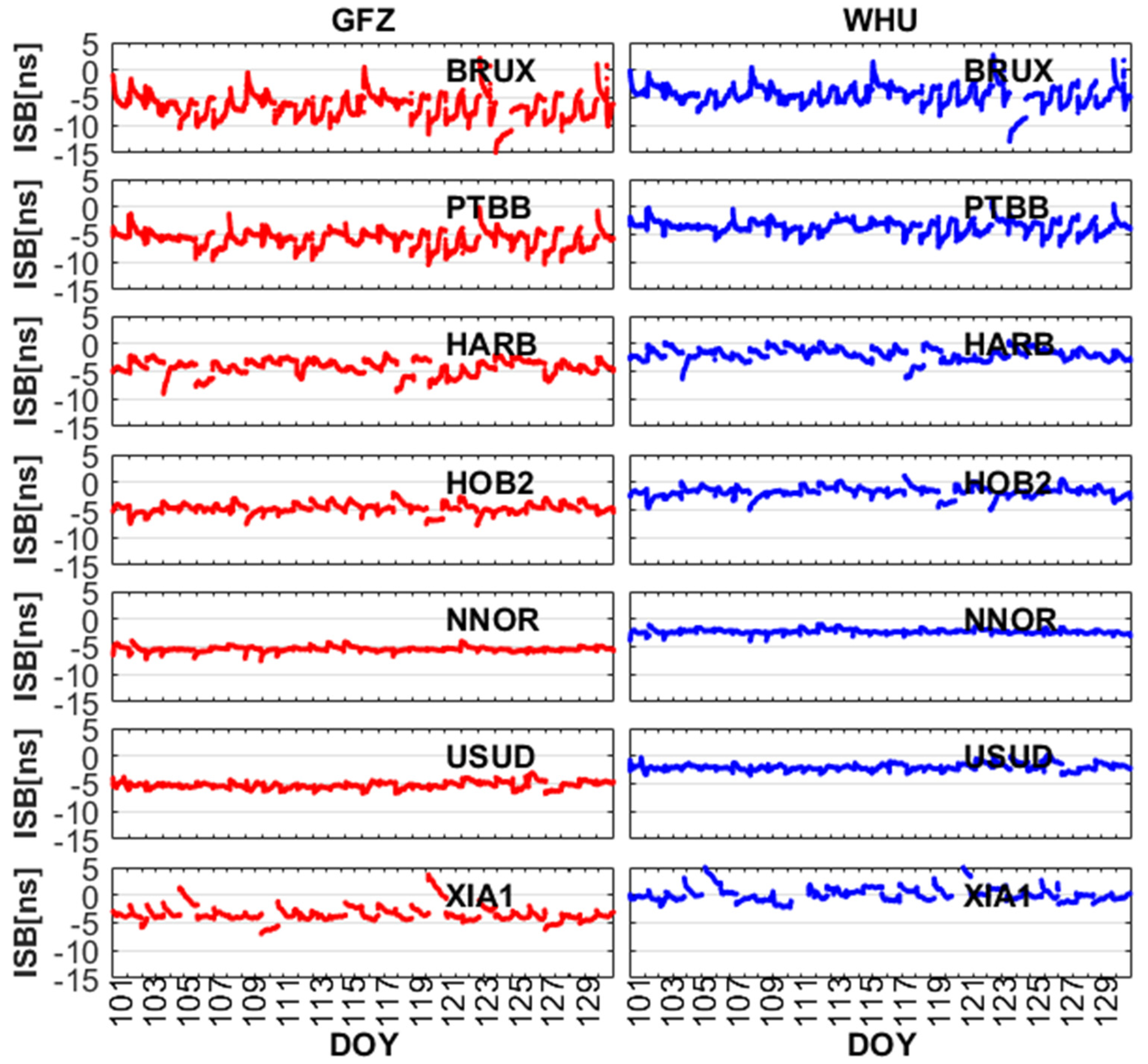
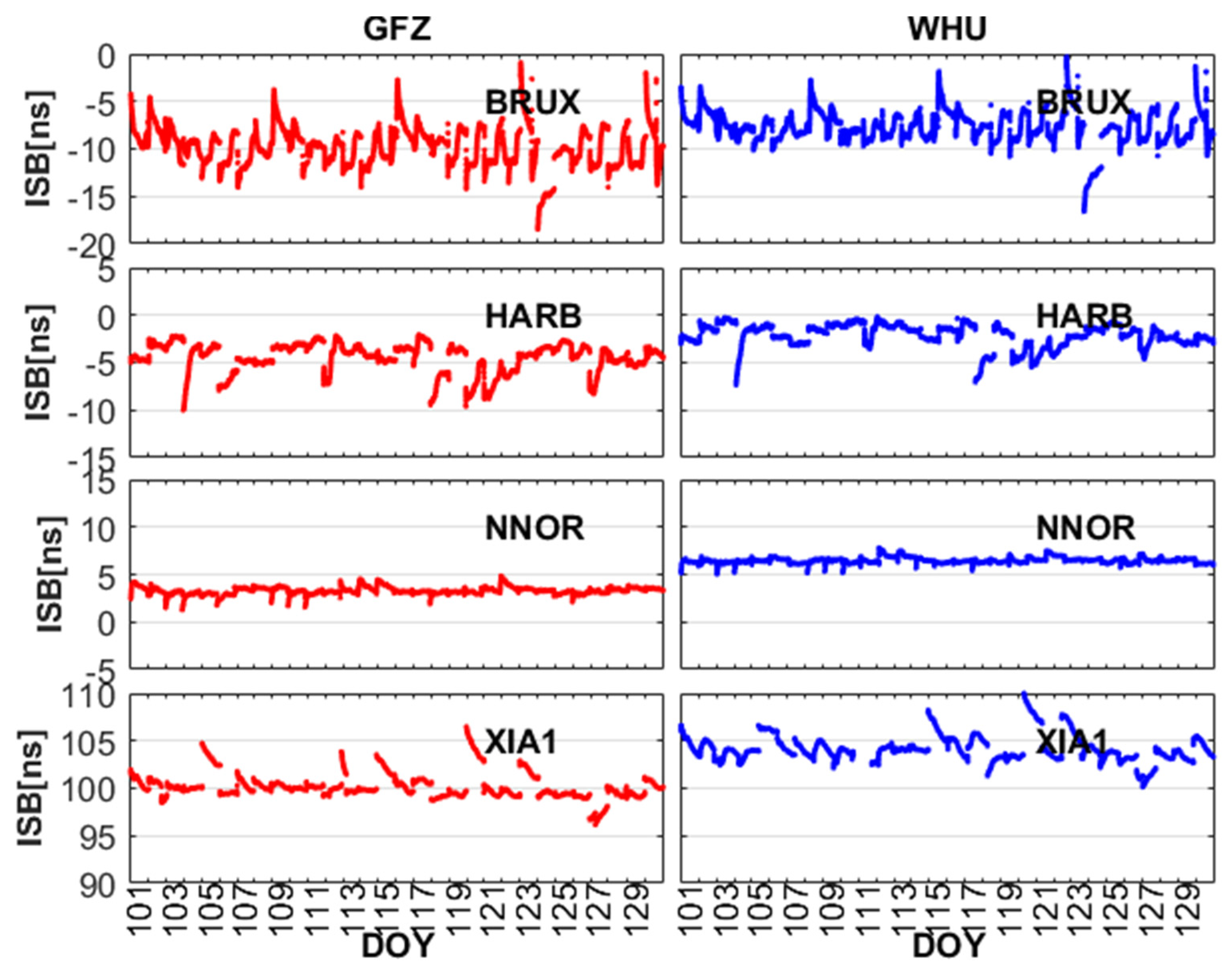
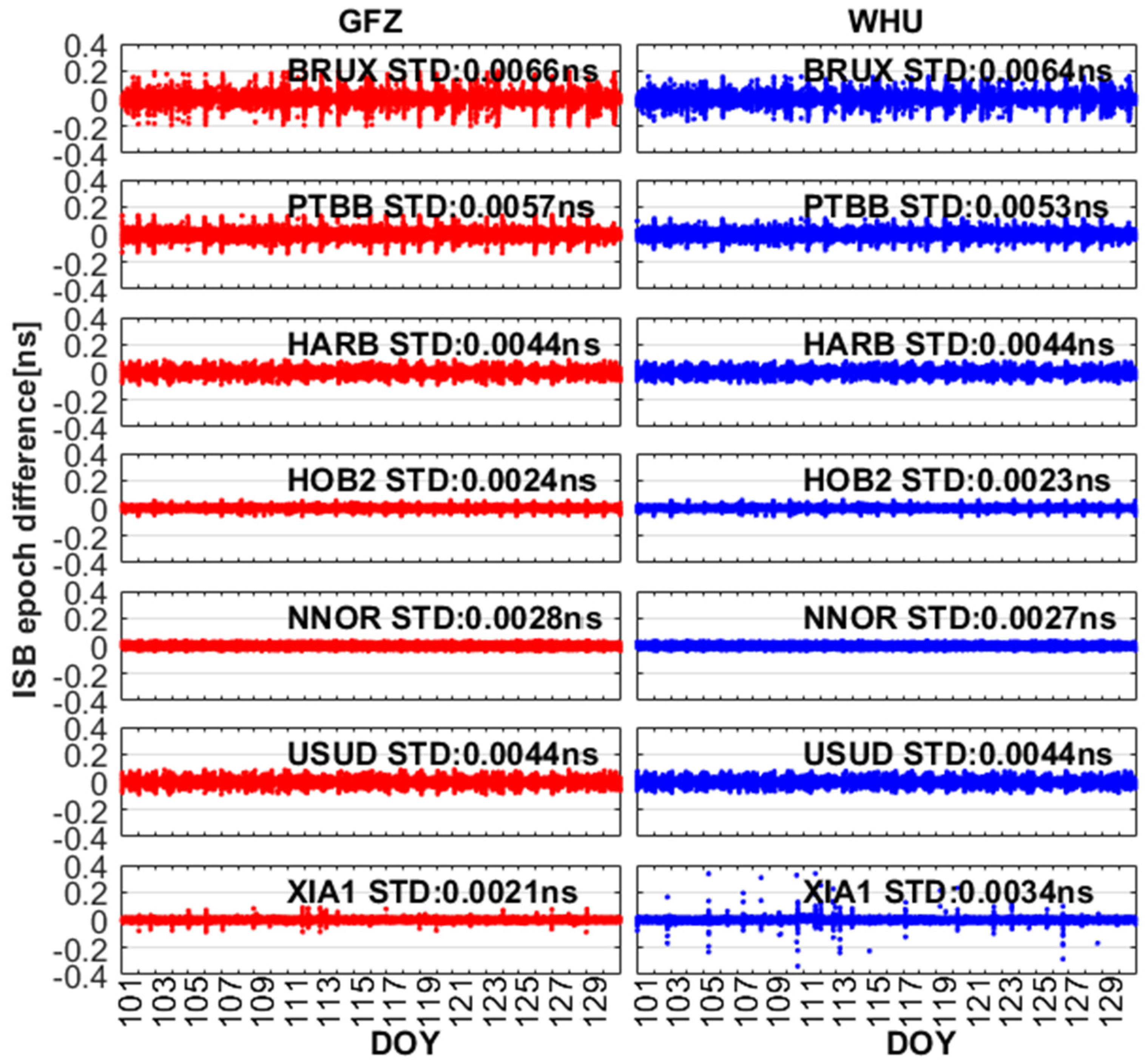
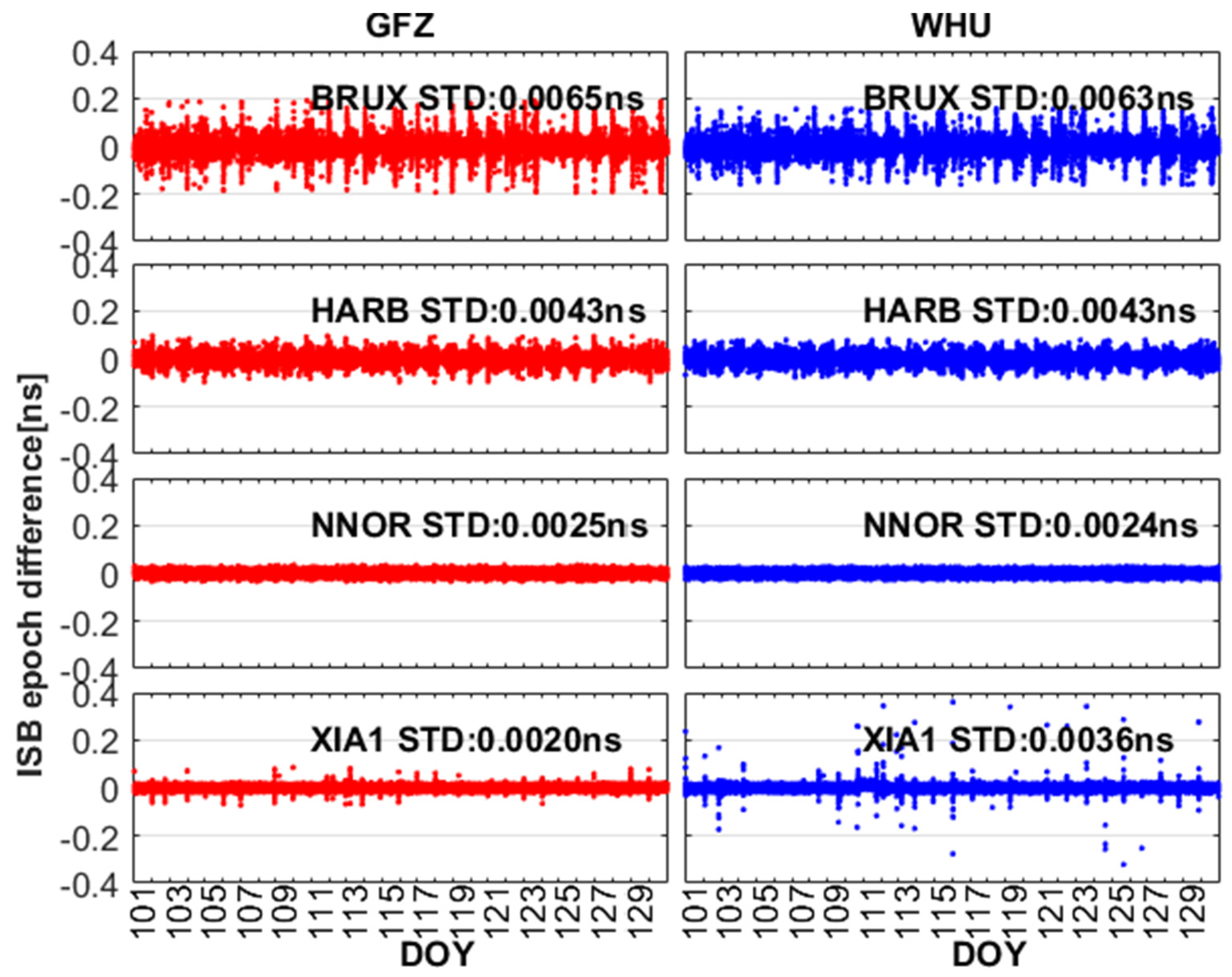
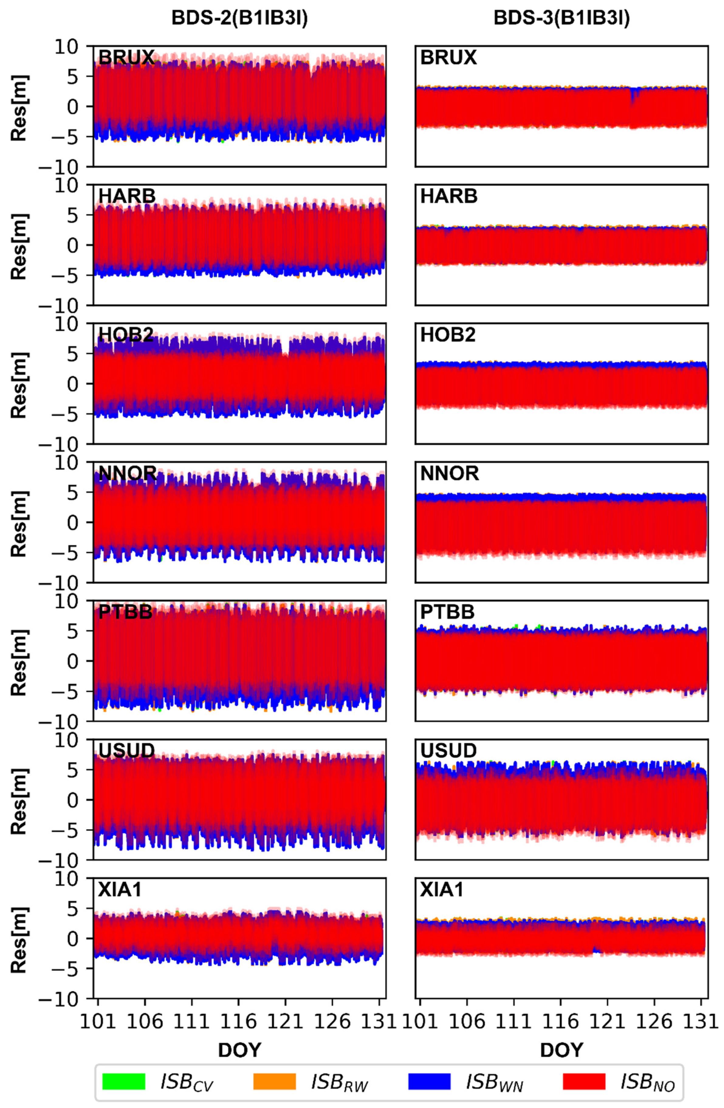
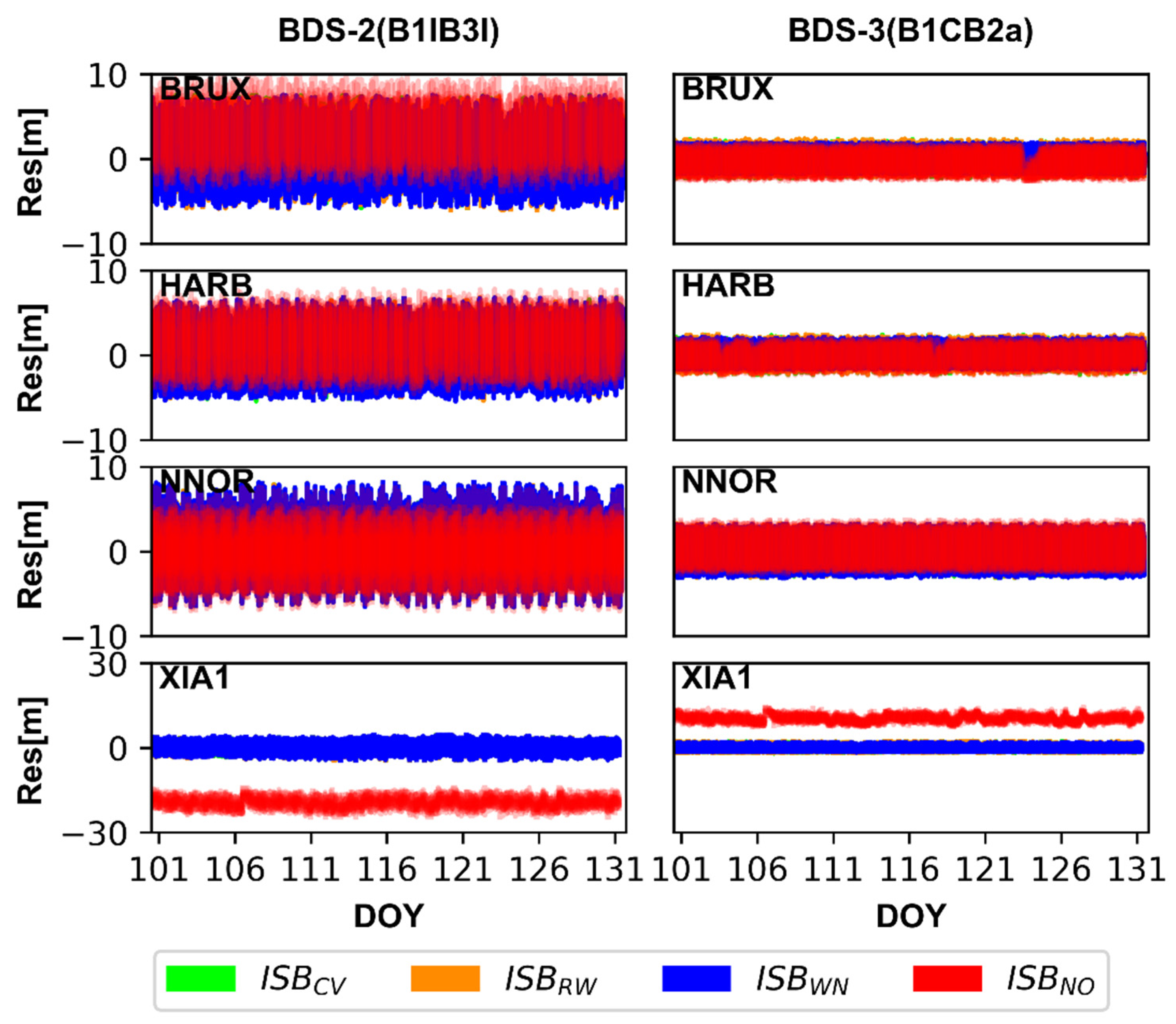
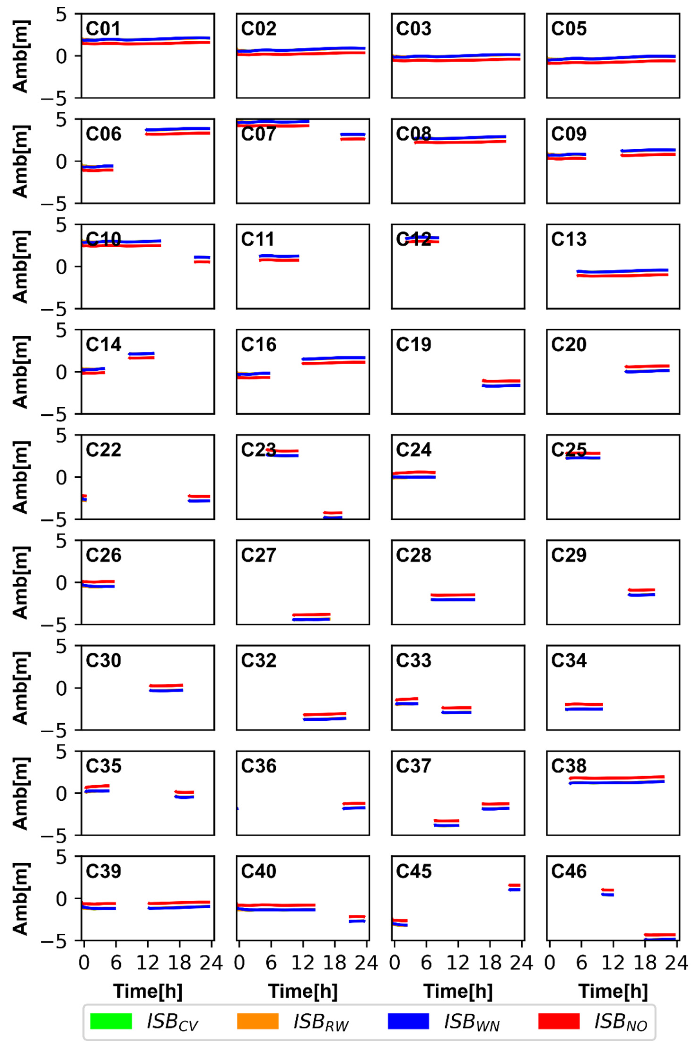
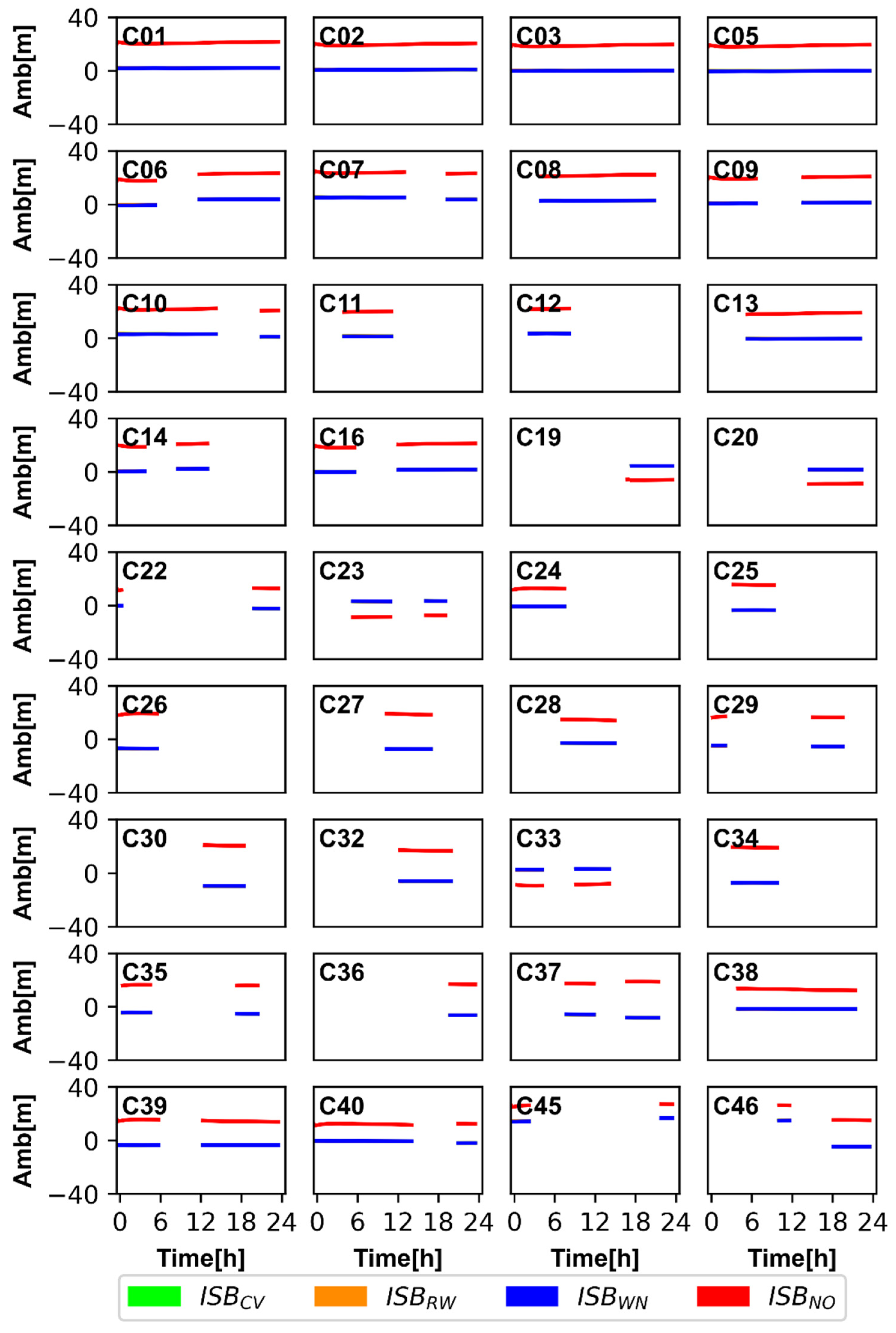
4.1. The Characteristic of ISB between BDS-2 and BDS-3

In order to prove that there is ISB between BDS-2 and BDS-3 for both new signals (B1C/B2a) and old signals (B1I/B3I), we compared the BDS-2-only and BDS-3-only estimated receiver clock offsets. As depicted in Figure 4, there are obvious differences between BDS-2 and BDS-3 for both the old signals (B1I/B3I) and new signals (B1C/B2a) in terms of receiver clock offsets. In the process of PCE, there is a difference between GFZ and WHU in the selection of reference station, which leads to the differences in receiver clock estimates. However, the differences between BDS-2 and BDS-3 are still very obvious for both GFZ and WHU products.

For BDS-2 (B1I/B3I) and BDS-3 (B1I/B3I), the signal modulations and characteristics have been adjusted and upgraded, which results in the difference in receiving and processing BDS-2 (B1I/B3I) and BDS-3 (B1I/B3I) signals. Due to the inconsistency between BDS-2 and BDS-3 in terms of the hardware units and the baseband algorithms on receiver side, we have to consider the ISB when B1I and B3I signals are used to perform BDS-2 and BDS-3 combined PPP solutions. Now turning to the new signals (B1C/B2a), the difference of frequency between new and old signals will inevitably produce the bias on receiver side, and the receiver clock offsets of BDS-2 and BDS-3 has obvious systematic bias. Figure 5 and Figure 6 depict the ISB between BDS-2 and BDS-3 for the old signals and new signals, respectively. By combining Figure 4 and Figure 5, we can determine that there are obvious ISB between BDS-2 (B1I/B3I) and BDS-3 (B1I/B3I). In addition, it can be seen from Figure 4 and Figure 6 that there is also an obvious ISB between BDS-2 (B1I/B3I) and BDS-3 (B1C/B2a). To describe the ISB of old and new signals more clearly, ISB_B1IB3I and ISB_B1CB2a represent ISB between BDS-2 (B1I/B3I) and BDS-3 (B1I/B3I) and ISB between BDS-2 (B1I/B3I) and BDS-3 (B1C/B2a), respectively. The statistics of ISB_B1IB3I and ISB_B1CB2a at the selected GNSS tracking stations from DOY 101 to 130 are listed in

Table 4. Statistics of ISB between BDS-2 and BDS-3 from DOY 101 to 130.

ISB	Station		GFZ			WHU
		Mean	STD	RMS	Mean	STD	RMS
BDS-2(B1I/B3I)/ BDS-3(B1I/B3I)	BRUX	−6.53 ns	1.36 ns	6.77 ns	−4.40 ns	1.06 ns	4.60 ns
	PTBB	−5.77 ns	0.93 ns	5.90 ns	−3.53 ns	0.70 ns	3.63 ns
	HARB	−4.16 ns	0.56 ns	4.20 ns	−1.83 ns	0.53 ns	1.96 ns
	HOB2	−4.77 ns	0.46 ns	4.77 ns	−1.76 ns	0.46 ns	1.80 ns
	NNOR	−5.43 ns	0.23 ns	5.43 ns	−2.23 ns	0.23 ns	2.23 ns
	USUD	−5.00 ns	0.26 ns	5.07 ns	−1.70 ns	0.30 ns	2.00 ns
	XIA1	−3.56 ns	0.40 ns	3.73 ns	0.13 ns	0.43 ns	1.10 ns
BDS-2(B1I/B3I)/ BDS-3(B1C/B2a)	BRUX	−9.70 ns	1.43 ns	9.87 ns	−7.60 ns	1.06 ns	7.70 ns
	HARB	−4.40 ns	0.53 ns	4.46 ns	−2.10 ns	0.40 ns	2.13 ns
	NNOR	3.23 ns	0.23 ns	3.26 ns	6.43 ns	0.16 ns	6.47 ns
	XIA1	99.96 ns	0.36 ns	99.96 ns	103.97 ns	0.56 ns	103.97 ns

. The mean of ISB_B1IB3I for GFZ and WHU range from −6.53 ns to −3.56 ns and −4.40 ns to 0.13 ns, and the root mean square (RMS) of ISB_B1IB3I for GFZ and WHU range from 3.73 ns to 6.77 ns and 1.10 ns to 4.60 ns. The mean of ISB_B1CB2a for GFZ and WHU range from −9.70 ns to 3.23 ns and −7.60 ns to 6.43 ns, the RMS of ISB_B1CB2a for GFZ and WHU range from 3.26 ns to 9.87 ns and 2.13 ns to 7.70 ns, except for XIA1. The receiver of XIA1 is obtained from the 20th Research Institute of China Electronics Technology Group Corporation (CETC-20). The receiver technology and manufacturing level are slightly worse than the receivers used by IGS. Therefore, there is a large difference between XIA1 and other stations in the mean and RMS of ISB_B1CB2a. The stability of ISB_B1IB3I and ISB_B1CB2a is good for all selected stations. The standard deviation (STD) at other stations is better than 1 ns, except for BRUX. Due to the difference of frequency and the signals processing strategy of receiver between new signals and old signals, ISB_B1IB3I and ISB_B1CB2a are quite different at the same station. In addition, we can find that there is a systematic bias of about 2–3 ns between using GFZ and WHU products. As mentioned above, there are differences between GFZ and WHU in the PCE strategy and the selection of reference stations. As depicted in Equation (8), the $\mathrm{d}{\mathrm{D}}^{\mathrm{C}3}-\mathrm{d}{\mathrm{D}}^{\mathrm{C}2}$ using GFZ products is different from WHU, which leads to systematic bias in ISB between using GFZ and WHU products.

To observe the variation of ISB_B1IB3I and ISB_B1CB2a, the epoch-differenced ISB are shown in Figure 7 and Figure 8. The epoch-differenced ISB_B1IB3I and ISB_B1CB2a are basically around 0. The STDs of ISB_B1IB3I for GFZ and WHU are (0.0066, 0.0057, 0.0044, 0.0028, 0.0044, 0.0021) ns and (0.0064, 0.0053, 0.0044, 0.0023, 0.0027, 0.0044, 0.0034) ns at the BRUX, PTBB, HARB, HOB2, NNOR, USUD, and XIA1 stations. The STDs of ISB_B1CB2a are (0.0065, 0.0043, 0.0025, 0.0020) ns and (0.0063, 0.0043, 0.0024, 0.0036) ns at the BRUX, HARB, NNOR, and XIA1 stations, respectively. This confirms the previous view that the stability of ISB_B1IB3I and ISB_B1CB2a are excellent.

ISB_B1IB3I and ISB_B1CB2a can be absorbed by receiver clock offsets, ambiguities, and observation residuals because of their strong correlation according Equation (7). Roughly speaking, ignoring the ISB will destroy the datum of receiver clock offsets and lead to the bias of the receiver clock offsets between BDS-2 and BDS-3, and confuse the time datum for time-frequency users, which is verified in Figure 4. In addition, ISB will also affect ambiguity and residuals. To illustrate it, the IF pseudo-range observation residuals and ambiguities of BDS-2 and BDS-3 satellites for the four ISB stochastic models are shown in Figure 9, Figure 10, Figure 11 and Figure 12. For the purpose of saving space and the results of WHU and GFZ are basically similar. Therefore, we only give the results based on GFZ products. We have two key findings from Figure 9 and Figure 10. First, the residuals of BDS-2 and BDS-3 for ISB_CV, ISB_RW, and ISB_WN are around 0, and the residuals of BDS-3 is obviously smaller than that of BDS-2. Second, the residuals of BDS-2 and BDS-3 for ISB_CV, ISB_RW and ISB_WN are closed and almost overlapped in Figure 9 and Figure 10. In order to more intuitively depict the residuals for each ISB models, the mean and STD of the residuals are shown in

Table 5. The mean and STDs of observation residuals of BDS-2 (B1I/B3I) and BDS-3 (B1I/B3I) satellites for four ISB stochastic models based on GFZ products.

Items	Station	BDS-2 (B1I/B3I)				BDS-3 (B1I/B3I)
		ISBNO	ISBCV	ISBRW	ISBWN	ISBNO	ISBCV	ISBRW	ISBWN
Mean	BRUX	2.11 m	0.86 m	0.77 m	0.61 m	−0.33 m	−0.03 m	0.02 m	0.03 m
	PTBB	2.05 m	0.88 m	0.83 m	0.73 m	−0.26 m	0.09 m	0.12 m	0.11 m
	HARB	1.53 m	0.60 m	0.60 m	0.58 m	−0.34 m	−0.06 m	−0.05 m	−0.06 m
	HOB2	1.16 m	0.50 m	0.50 m	0.50 m	−0.74 m	0.01 m	0.01 m	0.01 m
	NNOR	0.93 m	0.33 m	0.32 m	0.33 m	−1.04 m	0.01 m	0.02 m	0.01 m
	USUD	0.91 m	0.25 m	0.24 m	0.24 m	−0.87 m	0.03 m	0.05 m	0.04 m
	XIA1	0.50 m	−0.07 m	−0.07 m	−0.07 m	−0.48 m	0.06 m	0.07 m	0.04 m
STD	BRUX	1.62 m	1.62 m	1.62 m	1.65 m	0.71 m	0.71 m	0.71 m	0.66 m
	PTBB	2.04 m	2.04 m	2.04 m	2.05 m	1.25 m	1.25 m	1.25 m	1.25 m
	HARB	1.27 m	1.27 m	1.27 m	1.29 m	0.72 m	0.72 m	0.72 m	0.70 m
	HOB2	1.07 m	1.07 m	1.07 m	1.07 m	0.83 m	0.83 m	0.83 m	0.82 m
	NNOR	1.08 m	1.08 m	1.08 m	1.08 m	0.99 m	0.99 m	0.99 m	0.99 m
	USUD	1.26 m	1.26 m	1.26 m	1.26 m	1.04 m	1.04 m	1.04 m	1.01 m
	XIA1	1.04 m	1.04 m	1.03 m	1.03 m	0.80 m	0.80 m	0.79 m	0.78 m

and

Table 6. The mean and STDs of observation residuals of BDS-2 (B1I/B3I) and BDS-3 (B1C/B2a) satellites for four ISB stochastic models based on GFZ products.

Items	Station	BDS-2 (B1I/B3I)				BDS-3 (B1C/B2a)
		ISBNO	ISBCV	ISBRW	ISBWN	ISBNO	ISBCV	ISBRW	ISBWN
Mean	BRUX	3.10 m	0.86 m	0.76 m	0.61 m	−0.31 m	−0.02 m	0.01 m	0.01 m
	HARB	1.64 m	0.64 m	0.62 m	0.57 m	−0.12 m	0.05 m	0.08 m	0.09 m
	NNOR	−0.46 m	0.34 m	0.33 m	0.34 m	0.47 m	−0.01 m	0.02 m	0.01 m
	XIA1	−19.72 m	−0.08 m	−0.08 m	−0.07 m	10.30 m	0.06 m	0.05 m	0.03 m
STD	BRUX	1.62 m	1.62 m	1.62 m	1.66 m	0.48 m	0.47 m	0.47 m	0.43 m
	HARB	1.29 m	1.28 m	1.28 m	1.29 m	0.49 m	0.49 m	0.50 m	0.43 m
	NNOR	1.08 m	1.08 m	1.08 m	1.08 m	0.66 m	0.65 m	0.65 m	0.65 m
	XIA1	1.21 m	1.03 m	1.03 m	1.03 m	0.82 m	0.52 m	0.52 m	0.45 m

. Combining Figure 9 and Figure 10 and Table 5 and Table 6, we can conclude that the residuals of ISB_NO are obviously different from that of the other three models, and the difference is related to the ISB offsets. In other words, the greater the ISB offsets, the greater the difference between the residuals of ISB_NO and other models. For example, the ISB_B1CB2a of XIA1 is relatively large, and the difference between BDS-2 and BDS-3 is very obvious in residuals. In summary, ignoring ISB_B1IB3I and ISB_B1CB2a will cause the residuals to absorb the systematic error, which is related to the ISB offsets.

Now let us turn to Figure 11 and Figure 12; similar to the investigation of residuals, the ambiguities of BDS-2 and BDS-3 for ISB_CV, ISB_RW, and ISB_WN are very close to each other and almost overlapped in Figure 11 and Figure 12. The ambiguity of ISB_NO is obviously different from that of the other three models, and the difference is related to the ISB offsets. The ISB_B1CB2a of XIA1 is relatively large, and the difference of XIA1 is very obvious in ambiguities. The greater the ISB offsets, the greater the difference between the ambiguities of ISB_NO and other models. Based on the analysis of the impact of ISB on residuals and ambiguities, we can conclude that ignoring ISB_B1IB3I and ISB_B1CB2a will cause the residual and ambiguity to absorb the systematic error, which is related to the ISB offsets. Generally, estimating ISB between BDS-2 and BDS-3 can avoid the confusion of the datum of receiver clock offsets and avoid biasing residual and ambiguity.

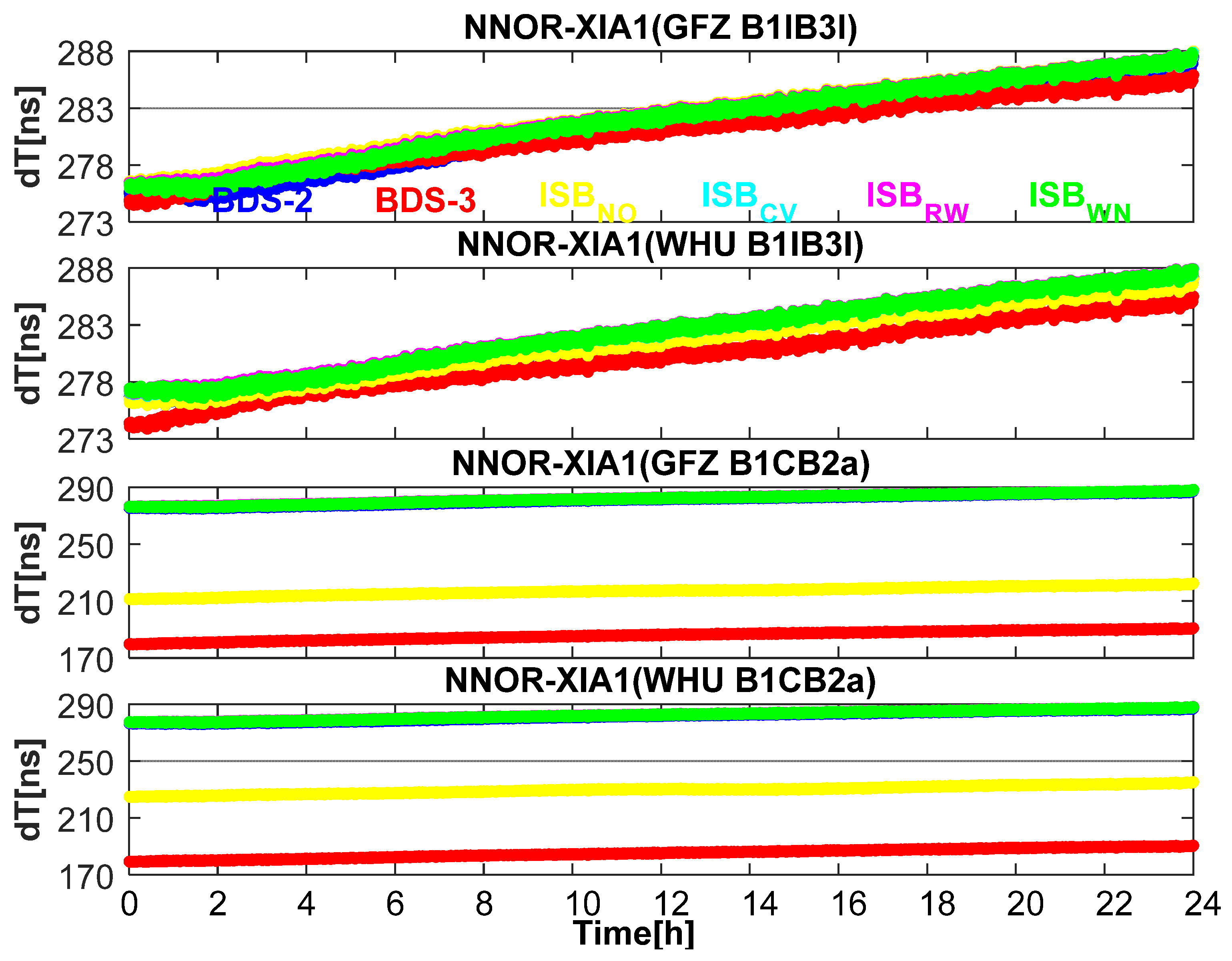
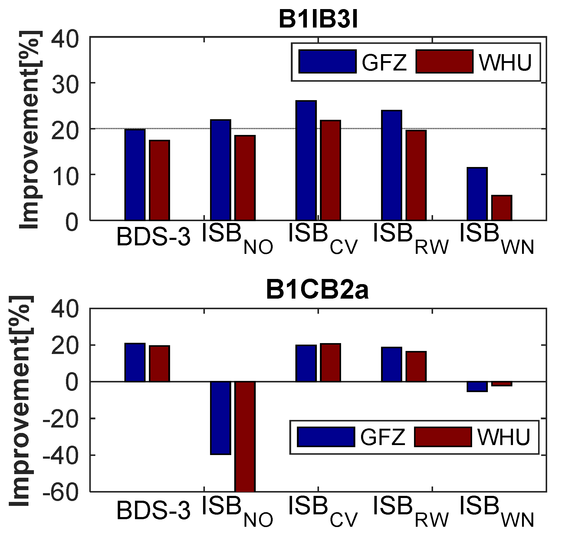
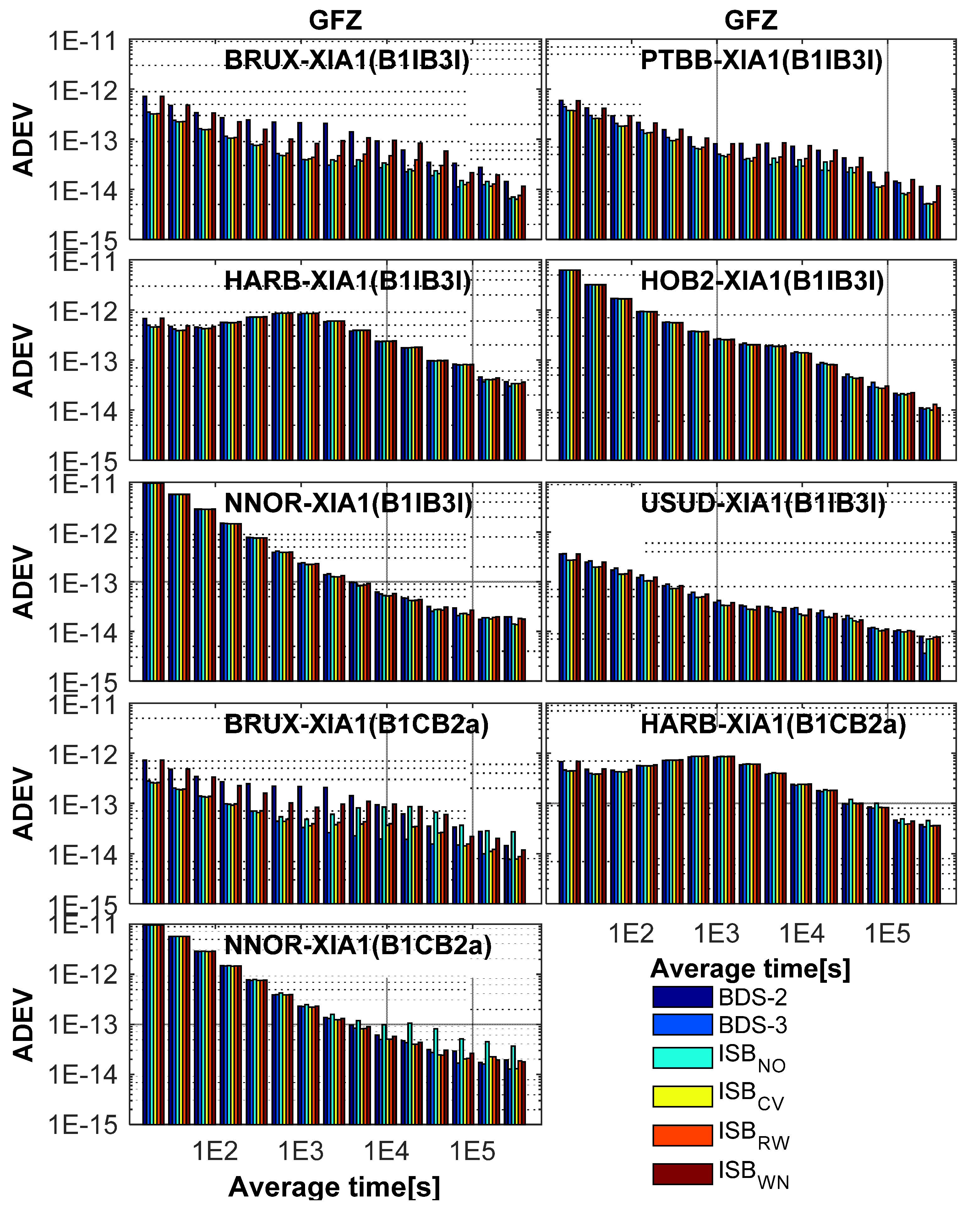
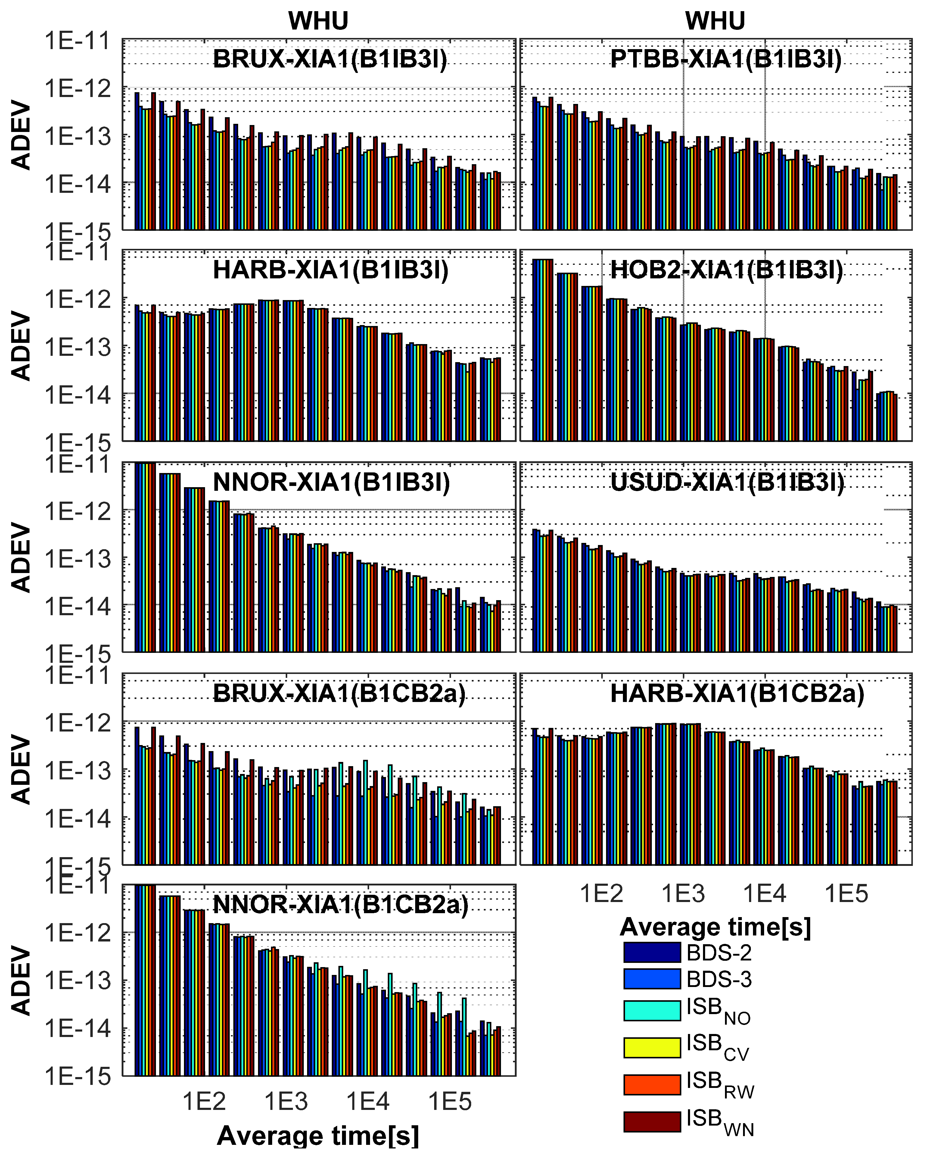
4.2. Precise Time and Frequency Transfer Using Different ISB Stochastic Models

Now we evaluate the impact of different ISB stochastic models on the BDS-2 and BDS-3 combined precise time and frequency transfer. Figure 13 depicts the one-day clock differences of BDS-2-only, BDS-3-only, and BDS for the four ISB stochastic models on the time-link NNOR-XIA1. Due to the existence of ISB, the datum of receiver clock offsets is destroyed. There is obvious stratification in the clock differences of BDS-2-only, BDS-3-only, and BDS (BDS-2/BDS-3). Moreover, the greater the ISB offsets, the greater the clock differences between BDS-2-only, BDS-3-only, and BDS (BDS-2/BDS-3). Most notably, estimating ISB can better eliminate this phenomenon, and the clock differences using ISB_CV, ISB_RW, and ISB_WN models are close and almost overlapped in Figure 13.

In order to assess the stability of clock differences using different ISB stochastic models, we compared the BDS clock differences and the GPS clock differences of the IGS final products on the established time-links.

Table 7. The STD of the differences between BDS clock differences and GPS clock differences of the IGS final product from DOY 101 to 130.

Agency /Frequency	Strategy	BRUX-XIA1	PTBB-XIA1	HARB-XIA1	HOB2-XIA1	NNOR-XIA1	USUD-XIA1	Mean
GFZ (B1IB3I)	BDS-2–IGSGPS	1.58 ns	1.29 ns	0.85 ns	0.57 ns	0.77 ns	0.72 ns	0.96 ns
	BDS-3 –IGSGPS	0.78 ns	0.85 ns	0.80 ns	0.71 ns	0.79 ns	0.69 ns	0.77 ns
	ISBNO–IGSGPS	0.79 ns	0.89 ns	0.78 ns	0.61 ns	0.72 ns	0.72 ns	0.75 ns
	ISBCV–IGSGPS	0.76 ns	0.86 ns	0.78 ns	0.56 ns	0.67 ns	0.68 ns	0.71 ns
	ISBRW–IGSGPS	0.82 ns	0.87 ns	0.79 ns	0.57 ns	0.68 ns	0.69 ns	0.73 ns
	ISBWN–IGSGPS	1.10 ns	1.24 ns	0.84 ns	0.58 ns	0.70 ns	0.68 ns	0.85 ns
GFZ (B1CB2a)	BDS-3–IGSGPS	0.74 ns	-	0.84 ns	-	0.72 ns	-	0.76 ns
	ISBNO–IGSGPS	1.33 ns	-	1.40 ns	-	1.29 ns	-	1.34 ns
	ISBCV–IGSGPS	0.84 ns	-	0.80 ns	-	0.68 ns	-	0.77 ns
	ISBRW–IGSGPS	0.85 ns	-	0.82 ns	-	0.68 ns	-	0.78 ns
	ISBWN–IGSGPS	1.51 ns	-	0.88 ns	-	0.66 ns	-	1.01 ns
WHU (B1IB3I)	BDS-2-IGSGPS	1.39 ns	1.14 ns	0.87 ns	0.68 ns	0.75 ns	0.74 ns	0.92 ns
	BDS-3-IGSGPS	0.82 ns	0.89 ns	0.79 ns	0.73 ns	0.69 ns	0.68 ns	0.76 ns
	ISBNO–IGSGPS	0.87 ns	0.88 ns	0.78 ns	0.64 ns	0.68 ns	0.68 ns	0.75 ns
	ISBCV–IGSGPS	0.80 ns	0.84 ns	0.77 ns	0.62 ns	0.66 ns	0.66 ns	0.72 ns
	ISBR–IGSGPS	0.82 ns	0.85 ns	0.80 ns	0.64 ns	0.68 ns	0.67 ns	0.74 ns
	ISBWN–IGSGPS	1.31 ns	1.10 ns	0.83 ns	0.65 ns	0.70 ns	0.68 ns	0.87 ns
WHU (B1CB2a)	BDS-3-IGSGPS	0.74 ns	-	0.82 ns	-	0.68 ns	-	0.74 ns
	ISBNO–IGSGPS	1.51 ns	-	1.53 ns	-	1.43 ns	-	1.49 ns
	ISBCV–IGSGPS	0.77 ns	-	0.75 ns	-	0.67 ns	-	0.73 ns
	ISBRW–IGSGPS	0.82 ns	-	0.82 ns	-	0.68 ns	-	0.77 ns
	ISBWN–IGSGPS	1.31 ns	-	0.85 ns	-	0.68 ns	-	0.94 ns

shows the statistical results of the established time-links, and Figure 14 depicts the percentage improvement based on Table 7. Combined with Figure 14 and Table 7, we can obtain three key findings. First, BDS-3 has a great improvement, and the stability of clock difference is improved by about 20% compared to BDS-2. Second, BDS-2 and BDS-3 combined solution can give full play to the performance of BDS and further improve the stability. The proper ISB stochastic model can make the clock differences more stable, whereas an improper model will make the accuracy and stability worse. Due to the influence of BDS-2, ISB_WN is worse than BDS-3-only. Finally, ISB_CV performs slightly better than other stochastic models. The optimal model is ISB_CV, the suboptimal model is ISB_RW, and the worst is ISB_WN for both old and new signals. For ISB_B1IB3I, ISB_NO can also obtain the good stability of clock difference, however, it is not recommended as it could confuse the datum of receiver clock offsets and further affect the clock difference on the time-links.

Through contrastive analysis, the statistical results obtained from GFZ and WHU have good consistency, which fully proves the accuracy of the above conclusions.

In this contribution, the Allan deviation (ADEV) was used to assess the frequency stability of the time differences on the established time-links, and the Stable32 software (http://www.wriley.com/ (accessed on 10 December 2020)) was used to calculate ADEV. Figure 15 demonstrates the ADEV values of the clock differences for BDS-2-only, BDS-3-only, and BDS (BDS-2/BDS-3 using the four ISB stochastic models) using GFZ products from DOY 101 to 130, and Figure 16 depicts the results using WHU products.

The stabilities of the intervals shorter than 1000 s for BDS-2-only, BDS-3-only, and BDS (BDS-2/BDS-3) are basically the same, except for BRUX-XIA1 and PTBB-XIA1. Because BDS-2 service area is mainly concentrated in Asia-Pacific region, the number of visible satellites for BDS-2-only on BRUX and PTBB stations is small. Therefore, the stability of BDS-2-only is so much worse than that BDS-3-only and BDS (BDS-2/BDS-3) in terms of the stability of the intervals shorter than 1000 s. From Figure 15 and Figure 16, there is a significant difference in the stability of the intervals longer than 10,000 s. ISB_CV performs slightly better than other ISB stochastic models in terms of the stability of the intervals longer than 10,000 s. The advantages and disadvantages of the models can be better reflected in the stability of longer periods, and ISB_CV performs slightly better than other ISB stochastic models. Furthermore, the ISB_RW model also shows good stability, and the performance of ISB_WN model is poor. In order to more intuitively reflect the advantages and disadvantages of the model, Figure 17 illustrates the percentage improvement in ADEV. For BDS-2 and BDS-3 combined solutions, ISB_CV presents a significant improvement over BDS-2-only solution. The maximum improvement of ISB_CV for the old signals and new signals are up to 28.35% and 32.92%. The mean of BDS-3-only, ISB_NO, ISB_CV, ISB_RW, and ISB_WN are (17.32%, 20.30%, 21.84%, 19.06%, 2.95%) for the old signals and (28.31%, −11.11%, 24.85%, 21.93%, 3.59%) for new signals.

As previously described for the actual situation of ISB varieties, the stability of ISB_B1IB3I and ISB_B1CB2a are excellent, and choosing a proper ISB stochastic model can achieve the best accuracy and stability of precise time and frequency transfer. The practice in the BDS-2 and BDS-3 combined PPP is to estimate ISB as a random constant, which helps to increase the geometric strength of the PPP model. In summary, the optimal model is ISB_CV, the suboptimal model is ISB_RW, and the worst is ISB_WN for both old signals and new signals in terms of the stability of time and frequency transfer.

5. Conclusions and Discussion

This research focused on the characteristics of BDS-2 and BDS-3 for both old signals (B1I/B3I) and new signals (B1C/B2a) and proposed four ISB stochastic models (ISB_NO, ISB_CV, ISB_RW, and ISB_WN) to analyze the impact of the ISB on the BDS-2 and BDS-3 combined precise time and frequency transfer performance. Through the analysis of ISB characteristics and its influence on the BDS-2 and BDS-3 combined precise time and frequency transfer, we can draw the following conclusions.

Due to the inconsistency between BDS-2 and BDS-3 in terms of the hardware units and the baseband algorithms on receiver side, there is an obvious ISB on receiver side for both old signals and new signals. From the point of view of stability of ISB, both ISB_B1IB3I and ISB_B1CB2a are excellent, and their STDs are basically better than 1 ns. The epoch difference of ISB_B1IB3I and ISB_B1CB2a are basically around 0, and their STDs are all better than 0.0066 ns. The existence of ISB will affect receiver clock offsets, ambiguity estimates, and observation residuals. When ignoring the ISB, the datum of receiver clock offsets will be destroyed, the time datum will be confused for time-frequency users, and the systematic errors will be absorbed into the residuals and ambiguities. In other words, estimating ISB between BDS-2 and BDS-3 can avoid this confusion.

About BDS precise time and frequency transfer, adding BDS-3 observations can improve the stability of clock differences compared to BDS-2-only solutions. With respect to the effect of ISB on precise time and frequency transfer, the optimal model is ISB_CV, the suboptimal model is ISB_RW, and the worst is ISB_WN for both old signals and new signals. With regard to the stability of frequency transfer, ISB_CV is also the most efficient way among these stochastic models. The ADEV can improve by 21.84% and 24.85% over BDS-2-only for the old signals and new signals. ISB_CV model conforms to the varieties of ISB, which can achieve the better accuracy and stability of precise time and frequency transfer.

In summary, the optimal model is ISB_CV, the suboptimal model is ISB_RW, and the worst is ISB_WN for both old signals and new signals in terms of the stability of time and frequency transfer. We recommend the optimal ISB_CV or suboptimal ISB_RW model for the BDS-2 and BDS-3 combined time and frequency transfer.

References

1. Yang, Y.; Gao, W.; Guo, S.; Mao, Y.; Yang, Y. Introduction to BeiDou-3 navigation satellite system. Navigation 2019, 66, 7–18. [Google Scholar] [CrossRef] [Green Version]
2. Yang, Y.; Li, J.; Xu, J.; Tang, J.; Guo, H.; He, H. Contribution of the Compass satellite navigation system to global PNT users. Chin. Sci. Bull. 2011, 56, 2813–2819. [Google Scholar] [CrossRef] [Green Version]
3. Yang, Y.; Tang, J.; Montenbruck, O. Chinese Navigation Satellite Systems. In Springer Handbook of Global Navigation Satellite Systems; Teunissen, P.J.G., Montenbruck, O., Eds.; Springer International Publishing: Cham, Switzerland, 2017; pp. 273–304. [Google Scholar] [CrossRef]
4. Montenbruck, O.; Hauschild, A.; Steigenberger, P.; Hugentobler, U.; Teunissen, P.; Nakamura, S. Initial assessment of the COMPASS/BeiDou-2 regional navigation satellite system. GPS Solut. 2012, 17, 211–222. [Google Scholar] [CrossRef]
5. Lee, S.W.; Schutz, B.E.; Lee, C.-B.; Yang, S.H. A study on the Common-View and All-in-View GPS time transfer using carrier-phase measurements. Metrologia 2008, 45, 156–167. [Google Scholar] [CrossRef]
6. Petit, G.; Jiang, Z. GPS All in View time transfer for TAI computation. Metrologia 2008, 45, 35–45. [Google Scholar] [CrossRef]
7. Weiss, M.A.; Petit, G.; Jiang, Z. A comparison of GPS common-view time transfer to all-in-view. In Proceedings of the 2005 IEEE International Frequency Control. Symposium and Exposition, Vancouver, BC, Canada, 29–31 August 2005; pp. 324–328. [Google Scholar] [CrossRef]
8. Larson, K.M.; Levine, J. Carrier-phase time transfer. IEEE Trans. Ultrason. Ferroelectr. Freq. Control 1999, 46, 1001–1012. [Google Scholar] [CrossRef]
9. Defraigne, P.; Aerts, W.; Pottiaux, E. Monitoring of UTC(k)’s using PPP and IGS real-time products. GPS Solut. 2014, 19, 165–172. [Google Scholar] [CrossRef]
10. Defraigne, P.; Baire, Q. Combining GPS and GLONASS for time and frequency transfer. Adv. Space Res. 2011, 47, 265–275. [Google Scholar] [CrossRef]
11. Ge, Y.; Dai, P.; Qin, W.; Yang, X.; Zhou, F.; Wang, S.; Zhao, X. Performance of Multi-GNSS Precise Point Positioning Time and Frequency Transfer with Clock Modeling. Remote Sens. 2019, 11, 347. [Google Scholar] [CrossRef] [Green Version]
12. Zhang, P.; Tu, R.; Zhang, R.; Gao, Y.; Cai, H. Combining GPS, BeiDou, and Galileo Satellite Systems for Time and Frequency Transfer Based on Carrier Phase Observations. Remote Sens. 2018, 10, 324. [Google Scholar] [CrossRef] [Green Version]
13. Tu, R.; Zhang, P.; Zhang, R.; Liu, J.; Lu, X. Modeling and performance analysis of precise time transfer based on BDS triple-frequency un-combined observations. J. Geod. 2018, 93, 837–847. [Google Scholar] [CrossRef]
14. Su, K.; Jin, S. Triple-frequency carrier phase precise time and frequency transfer models for BDS-3. GPS Solut. 2019, 23, 1–12. [Google Scholar] [CrossRef]
15. Jiang, N.; Xu, Y.; Xu, T.; Xu, G.; Sun, Z.; Schuh, H. GPS/BDS short-term ISB modelling and prediction. GPS Solut. 2016, 21, 163–175. [Google Scholar] [CrossRef] [Green Version]
16. Tu, R.; Hong, J.; Zhang, P.; Zhang, R.; Fan, L.; Liu, J.; Lu, X. Multiple GNSS inter-system biases in precise time transfer. Meas. Sci. Technol. 2019, 30. [Google Scholar] [CrossRef]
17. CSNO. BeiDou Navigation Satellite System Signal in Space Interface Control Document Open Service Signal (Version 2.1); China Satellite Navigation Office (China): Beijing, China, 2016. [Google Scholar]
18. CSNO. BeiDou Navigation Satellite System Signal in Space Interface Control Document Open Service Signal B3I (Version 1.0); China Satellite Navigation Office (China): Beijing, China, 2018. [Google Scholar]
19. CSNO. BeiDou Navigation Satellite System Signal in Space Interface Control Document Open Service Signal B1I (Version 3.0); China Satellite Navigation Office (China): Beijing, China, 2019. [Google Scholar]
20. Lu, M.; Li, W.; Yao, Z.; Cui, X. Overview of BDS III new signals. Navigation 2019, 66, 19–35. [Google Scholar] [CrossRef] [Green Version]
21. Jiao, G.; Song, S.; Jiao, W. Improving BDS-2 and BDS-3 joint precise point positioning with time delay bias estimation. Meas. Sci. Technol. 2020, 31. [Google Scholar] [CrossRef]
22. Zhang, Y.; Kubo, N.; Chen, J.; Wang, J.; Wang, H. Initial Positioning Assessment of BDS New Satellites and New Signals. Remote Sens. 2019, 11, 1320. [Google Scholar] [CrossRef] [Green Version]
23. Qin, W.; Ge, Y.; Zhang, Z.; Su, H.; Wei, P.; Yang, X. Accounting BDS3–BDS2 inter-system biases for precise time transfer. Measurement 2020, 156. [Google Scholar] [CrossRef]
24. Montenbruck, O.; Steigenberger, P.; Hauschild, A. Multi-GNSS signal-in-space range error assessment–Methodology and results. Adv. Space Res. 2018, 61, 3020–3038. [Google Scholar] [CrossRef]
25. Deng, Z.; Ge, M.; Uhlemann, M.; Zhao, Q. Precise orbit determination of BeiDou satellites at GFZ. In Proceedings of the IGS Workshop, Pasadena, CA, USA, 23–27 June 2014; pp. 23–27. [Google Scholar]
26. Deng, Z.; Schuh, H. Improvement of multi-GNSS orbit and clock prediction at GFZ. In Proceedings of the EGU General Assembly Conference Abstracts, Vienna, Austria, 4–13 April 2018; p. 2017. [Google Scholar]
27. Ge, M.; Chen, J.; Douša, J.; Gendt, G.; Wickert, J. A computationally efficient approach for estimating high-rate satellite clock corrections in realtime. GPS Solut. 2011, 16, 9–17. [Google Scholar] [CrossRef]
28. Guo, J.; Xu, X.; Zhao, Q.; Liu, J. Precise orbit determination for quad-constellation satellites at Wuhan University: Strategy, result validation, and comparison. J. Geod. 2015, 90, 143–159. [Google Scholar] [CrossRef]
29. Wang, C.; Zhao, Q.; Guo, J.; Liu, J.; Chen, G. The contribution of intersatellite links to BDS-3 orbit determination: Model refinement and comparisons. Navigation 2019, 66, 71–82. [Google Scholar] [CrossRef] [Green Version]
30. Bock, H.; Dach, R.; Jäggi, A.; Beutler, G. High-rate GPS clock corrections from CODE: Support of 1 Hz applications. J. Geod. 2009, 83, 1083–1094. [Google Scholar] [CrossRef] [Green Version]
31. Hadas, T.; Krypiak-Gregorczyk, A.; Hernández-Pajares, M.; Kaplon, J.; Paziewski, J.; Wielgosz, P.; Garcia-Rigo, A.; Kazmierski, K.; Sosnica, K.; Kwasniak, D.; et al. Impact and Implementation of Higher-Order Ionospheric Effects on Precise GNSS Applications. J. Geophys. Res. Solid Earth 2017, 122, 9420–9436. [Google Scholar] [CrossRef]
32. Odijk, D.; Teunissen, P.J.G. Characterization of between-receiver GPS-Galileo inter-system biases and their effect on mixed ambiguity resolution. GPS Solut. 2012, 17, 521–533. [Google Scholar] [CrossRef]
33. Rebischung, P.; Schmid, R. IGS14/igs14.atx: A new framework for the IGS products. In Proceedings of the AGU Fall Meeting 2016, San Francisco, CA, USA, 12–16 December 2016; Volume 121, pp. 6109–6131. [Google Scholar]
34. Wang, N.; Yuan, Y.; Li, Z.; Montenbruck, O.; Tan, B. Determination of differential code biases with multi-GNSS observations. J. Geod. 2015, 90, 209–228. [Google Scholar] [CrossRef]
35. Montenbruck, O.; Steigenberger, P.; Prange, L.; Deng, Z.; Zhao, Q.; Perosanz, F.; Romero, I.; Noll, C.; Stürze, A.; Weber, G.; et al. The Multi-GNSS Experiment (MGEX) of the International GNSS Service (IGS)–Achievements, prospects and challenges. Adv. Space Res. 2017, 59, 1671–1697. [Google Scholar] [CrossRef]
36. Landskron, D.; Bohm, J. VMF3/GPT3: Refined discrete and empirical troposphere mapping functions. J. Geod. 2018, 92, 349–360. [Google Scholar] [CrossRef] [PubMed]
37. Wanninger, L.; Beer, S. BeiDou satellite-induced code pseudorange variations: Diagnosis and therapy. GPS Solut. 2014, 19, 639–648. [Google Scholar] [CrossRef] [Green Version]
38. Yang, Y.; Xu, Y.; Li, J.; Yang, C. Progress and performance evaluation of BeiDou global navigation satellite system: Data analysis based on BDS-3 demonstration system. Sci. China Earth Sci. 2018, 61, 614–624. [Google Scholar] [CrossRef]
39. Su, K.; Jin, S.; Hoque, M. Evaluation of Ionospheric Delay Effects on Multi-GNSS Positioning Performance. Remote Sens. 2019, 11, 171. [Google Scholar] [CrossRef] [Green Version]
40. Kazmierski, K.; Sośnica, K.; Hadas, T. Quality assessment of multi-GNSS orbits and clocks for real-time precise point positioning. GPS Solut. 2017, 22, 1–12. [Google Scholar] [CrossRef] [Green Version]
41. Wu, J.-T.; Wu, S.C.; Hajj, G.A.; Bertiger, W.I.; Lichten, S.M. Effects of antenna orientation on GPS carrier phase. In Proceedings of the Astrodynamics 1991, San Diego, CA, USA, 19–22 August 1991; pp. 1647–1660. [Google Scholar]
42. Kouba, J. A Guide to Using International GNSS Service (IGS) Products; Jet Propulsion Laboratory: Pasadena, CA, USA, 2009; p. 34. [Google Scholar]
43. Petit, G.; Luzum, B. IERS Conventions (2010); IERS Technical Note No. 36; Verlag des Bundesamts für Kartographie und Geodäsie: Frankfurt am Main, Germany, 2010. [Google Scholar]
Figure 1. Distribution of the selected GNSS tracking station, in which the baselines denote the time-links.
Remotesensing 13 00793 g001
Figure 2. Global distribution of precision dilution of precision (PDOP) and time dilution of precision (TDOP) for BDS-2-only, BDS-3-only, and BeiDou global navigation satellite system (BDS) (BDS-2/BDS-3). The selected stations are also marked.
Remotesensing 13 00793 g002
Figure 3. Number of visible satellites for BDS-2-only, BDS-3-only, and BDS (BDS-2/BDS-3).
Remotesensing 13 00793 g003
Figure 4. The receiver clock offsets of BDS-2-only and BDS-3-only for new signals (B1C/B2a) and old signals (B1I/B3I) at stations BRUX (SEPT POLARX5TR), XIA1 (GNSS-GGR), and HOB2 (SEPT POLARX5).
Remotesensing 13 00793 g004
Figure 5. The inter-system bias (ISB) between BDS-2 (B1I/B3I) and BDS-3 (B1I/B3I) for Helmholtz Centre Potsdam German Research Center for Geosciences (GFZ) and Wuhan University (WHU) from DOY 101 to 130, 2020.
Remotesensing 13 00793 g005
Figure 6. The ISB between BDS-2 (B1I/B3I) and BDS-3 (B1C/B2a) for GFZ and WHU from DOY 101 to 130, 2020.
Remotesensing 13 00793 g006
Figure 7. The epoch-differenced ISB between BDS-2 (B1I/B3I) and BDS-3 (B1I/B3I) for GFZ and WHU from DOY 101 to 130, 2020.
Remotesensing 13 00793 g007
Figure 8. The epoch-differenced ISB between BDS-2 (B1I/B3I) and BDS-3 (B1C/B2a) for GFZ and WHU from DOY 101 to 130, 2020.
Remotesensing 13 00793 g008
Figure 9. The ionospheric-free (IF) pseudo-range observation residuals of BDS-2 (B1I/B3I) and BDS-3 (B1I/B3I) satellites for four ISB stochastic models based on GFZ products.
Remotesensing 13 00793 g009
Figure 10. The IF pseudo-range observation residuals of BDS-2 (B1I/B3I) and BDS-3 (B1C/B2a) satellites for four ISB stochastic models based on GFZ products.
Remotesensing 13 00793 g010
Figure 11. The ambiguities of BDS-2 (B1I/B3I) and BDS-3 (B1I/B3I) satellites for the four ISB stochastic models based on GFZ products at XIA1 station.
Remotesensing 13 00793 g011
Figure 12. The ambiguities of BDS-2 (B1I/B3I) and BDS-3 (B1C/B2a) satellites for four ISB stochastic models based on GFZ products at XIA1 station.
Remotesensing 13 00793 g012
Figure 13. The clock differences of BDS-2-only, BDS-3-only, and BDS (BDS-2/BDS-3 using the four ISB stochastic models) based on the time-link NNOR-XIA1 on DOY 114, 2020.
Remotesensing 13 00793 g013
Figure 14. Percentage improvement in the stability of BDS clock differences compared to BDS-2-only solution.
Remotesensing 13 00793 g014
Figure 15. Allan deviation (ADEV) of BDS-2-only, BDS-3-only, and BDS (BDS-2/BDS-3 using four ISB stochastic models) solutions using GFZ products from DOY 101 to 130, 2020.
Remotesensing 13 00793 g015
Figure 16. ADEV of BDS-2-only, BDS-3-only, and BDS (BDS-2/BDS-3 using four ISB stochastic models) solutions using WHU products from DOY 101 to 130, 2020.
Remotesensing 13 00793 g016
Figure 17. Percentage improvement in ADEV of BDS-3-only and BDS (BDS-2/BDS-3 using four ISB stochastic models) solutions compared BDS-2-only.
Remotesensing 13 00793 g017