Abstract
Nitrogen dioxide (NO2) is an important pollutant related to human activities, which has short-term and long-term effects on human health. An ensemble learning model was constructed and applied to estimate daily NO2 concentrations in the Beijing–Tianjin–Hebei region between 2010 and 2016. A variety of predictive variables included satellite-based troposphere NO2 vertical column concentration, meteorology, elevation, gross domestic product (GDP), population, land-use variables, and road network. The ensemble learning model achieved two things: a 0.01° × 0.01° grid resolution and the estimation of historical data for the years 2010–2013. The ensemble model showed good performance, whereby the R2 of tenfold cross-validation was 0.72 and the R2 of test validation was 0.71. Meteorological hysteretic effects were incorporated into the model, where the one-day lagged boundary layer height contributed the most. The annual NO2 estimation showed little change from 2010 to 2016. The seasonal NO2 estimation from highest to lowest occurred in winter, autumn, spring, and summer. In the annual maps and seasonal maps, the NO2 estimations in the northwest region were lower than those in the southeast region, and there was a heavily polluted band in the south of the Taihang Mountains. In coastal areas, the annual NO2 estimations were higher than the NO2 monitored values. The drawback of the model is underestimation at high values and overestimation at low values. This study indicates that the ensemble learning model has excellent performance in the simulation of NO2 with high spatial and temporal resolution. Furthermore, the research framework in this study can be a generally applied for drawing implications for other regions, especially for other cities in China.
1. Introduction
As an important air pollutant closely related to human activities, nitrogen dioxide (NO2) mainly derives from agricultural burning, traffic emissions, and industrial emissions [1,2,3]. Environmental epidemiological studies have shown that long-term and short-term NO2 exposure can lead to the exacerbation of respiratory and cardio-cerebrovascular diseases, as well as lung function damage, resulting in increased mortality and hospitalization rates [4,5,6,7]. Population exposure levels are usually obtained directly from NO2 monitoring sites, but monitoring sites are sparse and unevenly distributed, and they cannot effectively characterize NO2 concentration differences at fine scales. Meanwhile, the lack of historical monitoring data will limit the study of long-term health effects. Therefore, it is necessary to estimate long-term, full-coverage, and high-spatiotemporal-resolution NO2 concentrations to provide basic data for environmental epidemiological studies on NO2 exposure. The Beijing–Tianjin–Hebei region is the most serious NO2 pollution region in China, with high population density and high NO2 emissions [8]. Since the population has been exposed to high NO2 levels for a long time, there is a growing need for accurate NO2 estimation in the Beijing–Tianjin–Hebei region.
Various statistical methods have been used to construct models to calculate exposure to NO2 concentrations, evolving from linear regression models to nonlinear machine learning models. The essence of linear regression models is that the predictor variables and the dependent variable are linearly related, including land-use regression models [9,10,11,12], linear mixed-effects models [13], and geographically weighted regression models [14,15]. Land-use regression models focus on the spatial variation of pollutants, and they have been applied at spatial scales from global to urban [16]. Land-use models usually have high spatial resolution and low temporal resolution, mostly presented in terms of months, seasons, and years. Linear mixed-effects models focus on the effects of influencing factors on pollutant concentrations in time and tend to have a high temporal resolution of mostly daily and low spatial resolution, mostly 10 km × 10 km. Geographically weighted regression models are similar to linear mixed-effects models. Both land use models and linear mixed-effects models need to reach trade-offs in temporal and spatial resolution, whereby it is difficult to achieve both. In high-spatiotemporal-resolution air pollutant simulation, linear models cannot adequately express the relationship between the predicted variables and the monitored values of pollutant. In recent years, machine learning models have been applied and performed well. The estimation of air pollutants is already available at a temporal resolution of days and spatial resolution of 1 km × 1 km [13,17]. Machine learning models consider that there is a nonlinear relationship between predictor variables and dependent variables, including random forest models [18,19,20], gradient boosting tree models [17,21], and neural network models [17]. Compared with neural network models, random forest models are simple in structure, require less computational resources, and have stronger interpretation abilities. Random forest models provide the importance of variables to select the model predictor variables. The random forest model is also less prone to overfitting and less sensitive to outliers than the gradient boosting tree model.
Narrow land-use models only consider land-use types as predictor variables [22]. Broad land-use models also consider meteorological conditions, population density, elevation, road type and length, and coastal distance as predictor variables [23,24]. Some land-use models use satellite data as an important predictor variable [25,26,27]. Since its release in 2004, the tropospheric NO2 vertical column concentration inversion data provided by the Ozone Monitoring Instrument (OMI) have been widely used due to their high spatiotemporal resolution (13 × 24 km, daily), which enhances the seasonal and monthly performance of land-use models. Predictive variables of typical machine learning models in daily high-spatial-resolution air pollutant simulation (fine particulate matter (PM2.5), O3, NO2, SO2) studies usually include satellite data, meteorology, population density, elevation, road type and length, and land-use type variables [18,28,29,30,31,32,33,34]. Currently, there are still relatively few studies that built daily NO2 models for high spatial simulations of 0.01° × 0.01°, and the maximum spatial resolution for daily NO2 estimations is 0.1° × 0.1° in the Beijing–Tianjin–Hebei region [18].
The lack of historical data becomes a bottleneck problem in the long-term NO2 simulation studies. The NO2 monitoring network covering the whole country was only completed in China at the end of 2012. Long-term NO2 exposure levels are usually estimated with NO2 measurements over several years. In PM2.5 simulations, Chen et al. used monitoring values between 2013 and 2016 to estimate the lacking historical data from 2010–2012 [34]. Building statistical models with NO2 monitoring data over several years is a general way of bringing down annual variability and guaranteeing the accuracy of the estimation.
By constructing an ensemble learning model for 2010–2016 in the Beijing–Tianjin–Hebei region, this study aimed to (1) estimate the daily NO2 concentrations with a high spatial resolution of 0.01° × 0.01°, (2) incorporate satellite data, meteorological hysteretic effects, and the influence of human activities into model, (3) simulate the historical NO2 measurements from 2010 to 2012, and (4) describe the NO2 maps for 2010–2016. This study fills a gap by providing NO2 estimation at high spatial and temporal resolution in the Beijing–Tianjin–Hebei region, and it provides the necessary data for an environmental epidemiological study of the short-term and long-term health effects of NO2 exposure and air quality management on coordinated inter-regional prevention and control.
2. Materials and Methods
2.1. Study Area
The study area (113.45°–119.85° east (E), 36.03°–42.62° north (N)) was the Beijing–Tianjin–Hebei region in eastern China, located in the northern part of the North China Plain, with the Yanshan Mountains to the north, the Taihang Mountains to the west, and the Bohai Bay to the east. The topography is complex and diverse, with high altitudes in the northwest and low altitudes in the southeast. The Beijing–Tianjin–Hebei region includes Beijing, Tianjin, and 11 prefecture-level cities in Hebei Province: Hengshui, Xingtai, Handan, Qinhuangdao, Tangshan, Langfang, Baoding, Shijiazhuang, Cangzhou, Zhangjiakou, and Chengde. (Figure 1) With a high population (1.13 × 10⁸ people) and large area (2.18 × 10⁵ km2), the Beijing–Tianjin–Hebei study area has a developed transportation network and advanced economy; therefore, the NO2 levels are more than anywhere else across China. To eliminate the boundary effect, the study regional boundary was extended by 0.5° with respect to the overall study region (112.95°–120.35° E, 35.53°–43.12° N). The study period covered 1 January 2010–31 December 2016.
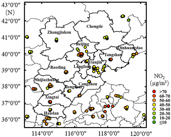
Figure 1.
Map showing 156 NO2 monitoring sites and the mean values of ground-based NO2 concentrations (μg/m3) in the study region from 2013 to 2016.
2.2. Datasets
2.2.1. Ground-Based NO2 Measurements
The ground-based daily NO2 measurements were collected from the China Environmental Monitoring Center (http://www.cnemc.cn/(accessed on 14 February 2021)) from 2010–2016. The study area contained a total of 156 state-controlled monitoring stations. Chemiluminescence was applied to measure the ground NO2 concentration for the monitoring sites. The mean values of the NO2 measurements for 2013–2016 at all sites are shown in Figure 1. The annual means and the descriptive statistical analysis of the NO2 monitoring values between 2013 and 2016 at all sites are shown in Figure S2 and Table S1 (Supplementary Materials).
2.2.2. Satellite Data
The OMI (Ozone Monitoring Instrument) on board the Aura satellite is a trace gas detector that can be used to accurately measure NO2. OMI provides daily global data at a local time of around 1:40 p.m. (https://search.earthdata.nasa.gov/ (accessed on 14 February 2021)). In this study, OMI tropospheric NO2 vertical column concentration level-3 global gridded data (OMI-NO2) from 1 January 2010 to 31 December 2016 were used [35]. The level-3 products are gridded OMI level-2 data averaged over a normalized grid (0.25° × 0.25°), mainly after the quality screening criteria of topographic reflectivity <30%, 0 ≤ solar zenith angle ≤ 85°, and a few row anomalies. OMI-NO2 data have missing values mainly due to the influence of clouds or high reflections from the ground. The overall absence rate was 34.46%, with the highest rate in winter (39.44%) and the lowest rate in summer (29.86%). Decision tree models were built to fill the missing values of OMI-NO2 and the performance of decision tree models is shown in Table S2 (Supplementary Materials).
2.2.3. Meteorological Data
The meteorological data for 2010–2016 were obtained from the ERA-interim (European Centre for Medium-Range Weather Forecasts Re-Analysis-Interim) reanalysis data of the mesoscale weather forecasts from the European Center (http://apps.ecmwf.int/datasets/data/interim-full-daily/levtype=sfc/ (accessed on 14 February 2021)). The spatial and temporal resolution of the daily near-surface meteorological data is 0.125° × 0.125° and 6/12 h. A total of 15 meteorological parameters are available, namely, atmospheric boundary layer height, low cloud cover, surface pressure, 2 m temperature, medium cloud cover, 2 m dew-point temperature, 10 m u wind, 10 m v wind, high cloud cover, downward surface solar radiation, surface evaporation, total precipitation, albedo, snowfall, and snow depth. The meteorological hysteresis effects were incorporated into model construction, whereas the 1 day and the 2 day lags of the meteorological data were also included in the model as important predictor variables.
2.2.4. Elevation Data, Population Data, and Gross Domestic Product (GDP) Data
The elevation, national population, and GDP data were collected from the Environmental Resource Science Data Center, the Chinese Academy of Sciences (RESDC) (http://www.resdc.cn (accessed on 14 February 2021)), in 2010, with a spatial resolution of 1 km × 1 km.
2.2.5. Land-Use Data
Land-use data were obtained from the European Space Agency’s Climate Change Initiative website for 2010–2016 (http://maps.elie.ucl.ac.be/CCI/viewer/ (accessed on 14 February 2021)). The spatial resolution of annual land-use data is 300 m. Data were gained from the 300 m Medium-Resolution Imaging Spectroradiometer (MERIS), reduced resolution products (RR), and full resolution products (FR), as well as the French Center for Space Research’s Earth Observation System, sensors AVHRR (Advanced Very High Resolution Radiometer) and PROBA-V (Airborne Autonomous Vegetation Program) mounted on NOAA’s (National Oceanic and Atmospheric Administration) meteorological satellites. The extracted land-use data can be divided into three types, namely, farmland coverage, natural vegetation coverage, and urban coverage.
2.2.6. Road Network Data
All road network data were obtained from the Resource and Environmental Science Data Center, the Chinese Academy of Sciences (RESDC) (http://www.resdc.cn (accessed on 14 February 2021)), which utilized the latest navigation map information. The road network consisted of national roads, provincial roads, county roads, township roads, highways, railroads, other vehicular roads, and footpaths. This study used data on country roads, county roads, provincial highways, national highways, railways, highways, and road density as road variables.
The classification, spatial resolution, temporal resolution, study time, and source of the dataset are shown in Table S3 (Supplementary Materials).
2.3. Data Processing
The whole study area extended by 0.5° was divided into a standardized grid with a spatial resolution of 0.01° × 0.01°, for a total of 560,180 grid cells. The datasets were resampled to the standardized grids by using the bilinear interpolation method. When calculating land-use coverage, a 0.03° × 0.03° grid was used as a buffer for the specified grid to calculate the land-use coverage of a certain type, and the proportion of that type of data was counted. The vector road data length was sliced through the standardized grid, and the final data were extracted to the standardized grid. In light of the latitude values and longitude values corresponding to each point, the data with ground-based NO2 measurements were extracted as the dataset required for model establishment. Data standardization was adopted in the data preprocessing to make data dimensionless that could be expressed as follows:
where X*, X, µ, and σ are the standardized value, the raw value, the mean value, and the standard deviation of the variables on the grid cell. ArcGIS and Python were used for data preprocessing and graphical plotting.
2.4. Modeling
Random forest, as a representative algorithm of the bagging method in the ensemble learning approach, is composed of several different and mutually independent decision trees [36]. The principle of ensemble learning methods is to combine weak evaluators into strong evaluators; therefore, ensemble learning methods perform better than a weak evaluator. For example, random forest usually performs better than a single decision tree. A decision tree is a forked structure where each internal node represents an attribute judgment, each branch represents the output of a judgment result, and each leaf node represents a classification result. Random forest generates a new set of training samples by repeatedly sampling k samples at random from the original training sample set N in a put-back manner through the self-service method resampling technique, and then generates k regression trees as a function of the self-service sample set. The results of the prediction data are determined by the average of different regression trees. The ground-level NO2 concentrations were simulated by building an ensemble learning model using the random forest method with the following expressions:
where NO2ij is the ground NO2 concentration on grid cell j and day i, OMI-NO2, MET, POP, ELE, ROD, and LU are the OMI-NO2, meteorological variables, population, GDP, elevation, road length and density, and the coverage rate of land-use types on grid cell j, and MET_lag1 and MET_lag2 are the 1 day lag and 2 day lag of the meteorological variables. The maximum depth (the depth of the tree) and n_estimators (the number of trees) were two important parameters for model adjustment. During model adjustments, the model had high prediction accuracy when the maximum depth and n_estimators were set to 50 and 200. The error rate of the model was calculated by predicting the out-of-bag samples.
An ensemble learning model was developed to estimate NO2 concentrations in the whole study area for 2010–2016, including the historical years of 2010–2012 without NO2 measurements. The scikit-learn package in Python was used to construct the model.
2.5. Validation
In this study, the tenfold cross-validation method and test set validation method were used to evaluate the model’s performance. The entire dataset was randomly divided into a training set and a test set with a ratio of 9:1. Tenfold cross-validation method involves dividing the data in the training set into 10 randomly equal parts, of which nine parts are used for the training of the model and the remaining part is used for the validation of the model; this process is performed 10 times, and the final validation result of the model is averaged over these 10 times. Test set validation is the validation of the model results when the whole training set is used for the training of the model. The indicators of model evaluation included the R2 value, mean absolute prediction error (MAE), and root-mean-square prediction error (RMSE). The R2 value was applied to the tenfold cross-validation (cv-R2) and the test validation (test-R2), whereas the MAE and RMSE were only included in the test set evaluation (test-MAE and test-RMSE).
3. Results
3.1. Descriptive Analysis
A total of 59 predictor variables and 160,371 modeled data were available in the NO2 model construction. The mean value and standard deviation value of NO2 concentrations at the monitoring stations were 46.80 µg/m3 and 26.91 µg/m3, respectively, which were significantly higher than 40 µg/m3. The annual mean guideline of the World Health Organization (WHO) and China’s GB 3095-2012 for NO2 is no more than 40 µg/m3 [37,38]; therefore, the study area was in a perennial pollution state between 2013 and 2016. The mean value of urban coverage was 81.3%, which meant that most of the locations of the currently collected monitoring data were concentrated in urban areas. The standard deviation value and mean value of OMI-NO2 were 23.44 × 10¹⁵ molecules/cm2 and 8.30 × 10¹⁵ molecules/cm2. The descriptive statistical analysis of these predictor variables is shown in Table S4 (Supplementary Materials). The variables such as GDP, population, and elevation are visualized in Figure S1 (Supplementary Materials).
3.2. Importance Percentage of Predictor Variables
The importance percentages of all predictor variables for the NO2 model are shown in Table S5 (Supplementary Materials). The summation of all variables was 1. The meteorological lag factor had a very high contribution to the importance of the variables, with the top five being all meteorological variables with 1 day lag and 2 day lag. The 1 day lagged atmospheric boundary layer height was the most important variable, contributing 29.9%. Furthermore, GDP, elevation, OMI-NO2, and population density contributed 1.6%, 1.6%, 1.5%, and 1.3%, respectively. However, the contributions of the various types of road data and land-use variables were less than 1%.
3.3. Temporal Performance
Figure 2 shows the daily-level simulation results of the estimations and measurements of NO2, where cv-R2 and test-R2 were 0.72 and 0.71. The daily-level performance of the model for the different years and seasons is shown in Figure 3, indicating the model’s stability on these time scales. The model’s test-R2 was 0.77 and 0.76 in 2016 and 2015, which is better than the 0.65 and 0.64 obtained in 2014 and 2013. The differences between years may be related to the number of the daily measurements for different years. The number of daily measurements showed an increasing trend year by year. As a result, the model performed best in 2016 and worst in 2013.The model’s test-R2 was different in the four seasons. The model performed best in winter with a test-R2 of 0.71, followed by autumn and spring with 0.67 and 0.65, and the worst performance was in summer with 0.53.
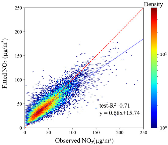
Figure 2.
Density scatter plot showing the daily-level model’s results of fitting and test set validation (N = 160,371). The red dashed line is a 1:1 line and the blue line is from the linear regression. Blue indicates that the number of dots is small and the density of dots is low; red indicates a high number of dots with a high density of dots.
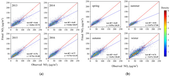
Figure 3.
Density scatter plots showing the daily-level model’s results of fitting and test set validation in different years (a) and seasons (b). The red dashed line is a 1:1 line and the blue line is from the linear regression. Blue indicates that the number of dots is small and the density of dots is low; red indicates a high number of dots with a high density of dots.
3.4. Spatial Performance
The performance of the model in different provinces (Hebei), municipalities (Beijing and Tianjin), and prefecture-level cities of Hebei is statistically shown in Table 1. According to the evaluation index test-R2, the model had the highest performance in Beijing (0.82), followed by Tianjin (0.77) and finally Hebei (0.72). According to the evaluation indices test-RMSE and test-MAE, the model had the lowest performance in Beijing (11.65 µg/m3 and 8.45 µg/m3), followed by Tianjin (11.91 µg/m3 and 8.76 µg/m3) and finally Hebei (15.14 µg/m3 and 10.33 µg/m3). Therefore, the overall performance of the model was best in Beijing, followed by Tianjin and finally Hebei. In the validation results of 11 prefecture-level cities, the model simulation results were the best in Xingtai, Hengshui, Shijiazhuang, and Tangshan, with a test-R2 higher than 0.7. However, the model performed worst in Handan, Cangzhou, and Qinhuangdao, with a test-R2 lower than 0.5. The model performed better in Beijing and Tianjin than in Hebei because the distribution density of monitoring stations in Beijing and Tianjin is much higher than that in Hebei. Due to the large number of monitoring stations in Beijing, Tianjin, Tangshan, Baoding, Shijiazhuang, Hengshui, and Xingtai, the model performed well in these places. Qinhuangdao and Cangzhou are far from these cities; thus, the model performed poorly in these two cities.

Table 1.
The model’s performance of the test set validation results in the whole region, different provinces (including municipalities), and 11 prefecture-level cities of Hebei. RMSE, root-mean-square error; MAE, mean absolute error.
3.5. Spatial and Temporal Distribution
The statistical analysis results based on model simulation are shown in Table S6 (Supplementary Materials). The daily NO2 estimation achieved the spatial resolution of 0.01° × 0.01°. Between 2010 and 2016, the annual mean NO2 estimation ranged from 46.72 µg/m3 to 47.63 µg/m3 in the Beijing–Tianjin–Hebei region. Therefore, the annual mean NO2 estimation from 2010 to 2016 did not vary much and was generally consistent with the monitored values. Figure 4 shows that the NO2 estimations of the southeast part of the study region were higher than those in the northwest part. There was a heavily polluted band to the south of the Taihang Mountains, where annual NO2 estimations were higher than 55µg/m3, including Beijing, Shijiazhuang, Xingtai, and Handan. High NO2 estimations also appeared in the coastal areas of Tianjin and Qinhuangdao. The annual NO2 estimated maps show similarity in spatial distribution to the annual NO2 monitored maps (Figure S2, Supplementary Materials).
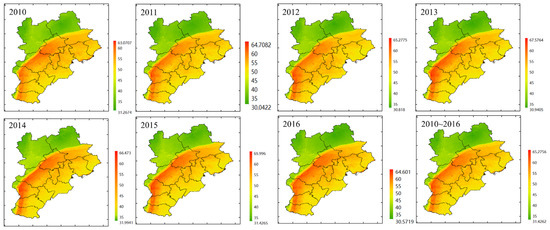
Figure 4.
The annual NO2 maps in the Beijing–Tianjin–Hebei region for 2010–2016. High values are represented by the red color and low values are represented by the green color. The unit of NO2 concentration in the legend is µg/m3.
Figure 5 shows the seasonal distribution of NO2 estimations from 2010 to 2016. In any season, the NO2 estimations in the northwest region were lower than those in the southeast region, and there was a heavily polluted band to the south of the Taihang Mountains, where NO2 estimations were higher than 55 µg/m3. There was a similar spatial distribution between the seasonal NO2 estimations and the annual NO2 estimations. In the southeast region, the heavily polluted bands from large to small occurred in winter, autumn, spring, and summer. The winter mean NO2 estimations for 2010–2016 were 49.05 µg/m3, 47.68 µg/m3, 47.77 µg/m3, 49.34 µg/m3, 49.42 µg/m3, 48.90 µg/m3, and 50.19 µg/m3 (Table S6, Supplementary Materials). From 2013 to 2016, the NO2 measurements in the southeastern region in winter were all higher than 60 µg/m3 (Table S7, Supplementary Materials), with similar results obtained for the NO2 estimations. The seasonal simulated values in autumn and winter in the northwestern region showed different results from those in the southeast for 2013–2016, whereby the seasonal simulated values in autumn were greater than those in winter. From the monitoring site, the seasonal simulated values in autumn were greater than those in winter from 2013 to 2014, and this difference lessened from 2014 to 2015; eventually, the seasonal simulated values in autumn were lower than those in winter from 2015 to 2016. Along the coast, seasonal variation was also different from that inland, showing high values in spring and summer and low values in autumn and winter, which was inconsistent with the nearby monitored values (Figure S3, Supplementary Materials).
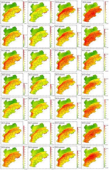
Figure 5.
The seasonal NO2 maps of different years in the study region for 2010–2016 estimated using the ensemble learning model. Spring includes March, April, and May; summer includes June, July, and August; autumn includes September, October, and November; winter includes December, January of the next year, and February of the next year. However, values for winter in 2016 only include December. High values are represented by the red color and low values are represented by the green color. The unit of NO2 concentration in the legend is µg/m3.
4. Discussion
An ensemble learning model was constructed and applied to estimate daily NO2 concentrations in the Beijing–Tianjin–Hebei region. This study achieved a spatial resolution of 0.01° × 0.01° (~1 km × 1 km) in the study area. The ensemble learning model achieved pretty good performance considering that cv-R2 and test-R2 were 0.72 and 0.71, respectively. Meteorological lag variables made great contributions to the model. Taking NO2 ground monitoring values from 2013 to 2016 as the dependent variable, a pervasive model was constructed to simulate the historical NO2 measurements between 2010 and 2012.
4.1. Comparsion with other NO2 Models
This study achieved the highest spatial resolution of 0.01° × 0.01° (~1 km × 1 km) in the Beijing–Tianjin–Hebei region, and the model performed better than those presented in the Zhan et al. study [18] and Qin et al. studies [14,19], with cv-R2 = 0.72 and RMSE = 14.35 µg/m3. Zhan et al. simulated daily NO2 concentrations across China from 2013 to 2016 by building a random forest spatiotemporal kriging model with a spatial resolution of 0.1° × 0.1° (~10 km × 10 km), with cv-R2 = 0.62 and RMSE = 13.3 µg/m3 [18]. Qin et al. simulated NO2 concentrations in the eastern region of China from March 2013 to April 2014 using a spatiotemporal geographically weighted regression (GTWR) model with a spatial resolution of 0.1° × 0.1°, with cv-R2 = 0.60 and RMSE = 9.38 µg/m3 [14]. Qin et al. simulated NO2 concentrations in the eastern region of China from December 2016 to November 2017 using a random forest (RF) model and an extreme random tree (ET) model with a spatial resolution of 0.25° × 0.25°, with cv-R2 = 0.69 and 0.70, and RMSE = 9.47 and 9.42 µg/m3 [19]. The NO2 simulations at high spatial resolution showed a greater range of variation and higher values of RMSE than those studied at low spatial resolution. Similar to the study by Zhan et al. [18], this study was simulated for historical missing data from 2010 to 2012, which is important for long-term health risk studies of NO2 exposure. Studies based on longer-scale monitoring data would accommodate more data and build more generalized models than studies using only short-term monitoring data to predict historical data. For example, in the PM2.5 estimations over the historical years, Zhao et al. used the monitoring values for 2013–2016 to estimate the historical monitoring values between 2010 and 2012 [34]. Ma et al. adopted the monitoring values of 2013 to estimate the long-term historical monitoring values lacking for 2004–2012 [39]. The study by Zhao et al. was better than the study by Ma et al. in the simulation of historical missing values over several years.
Compared with other NO2 simulation studies at the spatial resolution of 0.01° × 0.01°, our model performed better than the linear mixed-effects model (R2 = 0.56–0.64) used by de Hoogh et al. in their study across Switzerland [13], but worse than the random forest model (cv-R2 = 0.79), gradient boosting tree (cv-R2 = 0.75), neural network model (cv-R2 = 0.76), and their superposition (cv-R2 = 0.79) used by Di et al. in their study in the United States [17]. Among the applications of machine learning models, ensemble learning models were used more than other models, especially the random forest model. According to the generation method of the base learner, ensemble learning can be divided into two categories. One is the bagging method, which exploits the independence of the base learners, of which the outstanding representative is the random forest, and the other is the boosting method, which exploits the relevance of the base learners, of which an excellent representative is xgboost [40]. In this study, these two models were compared, where the xgboost model performed with cv-R2 = 0.70, test-R2 = 0.64, and RMSE = 16.13 µg/m3. The xgboost model was much less computationally intensive compared to the random forest model, but easily overfitted. Compared to neural network models, random forest models were less computationally intensive, simple in structure, and easy to tune and use. The ensemble learning models including random forest and xgboost provided the importance share of all predictor variables.
4.2. Predicator Variable Selection
There are three factors that affect NO2 concentration in the atmosphere: meteorology, topography, and emissions. In terms of meteorology, 15 possibly related meteorological variables were selected. Elevation was chosen as a representation of the terrain. Emission sources were divided into anthropogenic sources and natural sources, including land-use cover types, population, GDP, and road network. Land-use cover types have a significant impact on NO2 emissions [41]. Li et al. found that land-use cover types were important factors influencing the spatial pattern of NOx emissions in the Beijing–Tianjin–Hebei region except for Beijing [42]. In addition to land cover, there are other influencing factors in Beijing, such as industrial structure and pollution control level. As a result, GDP and population were also selected [43,44,45,46]. The amount of traffic emissions was represented by the type and density of the road network.
The data about the meteorological hysteresis effect were considered as important variables of the model and improved the performance of the model by ~0.02 in terms of cv-R2 and test-R2. Meteorological conditions affected the residual layer, which stored some NO2 and released it later. Therefore, this study used meteorological lagged data to represent the contribution of the residual layer. In the Zhao et al. study, meteorological lag conditions were incorporated into the model construction to estimate PM2.5 [34].
We found that the topography was also important, which may be due to the complex and variable topography in the Beijing–Tianjin–Hebei region. This model used variables to characterize emissions from human and natural sources, such as population, GDP, land-use types, and road types [43,44,45,46]. Among them, population and GDP had relatively important contributions to the model, but land-use variables and road variables were not as important as we might expect, mainly because the road data did not provide a good portrayal of the daily variation in traffic flow.
The contribution of OMI-NO2 to the model was 0.015; however, in the Qin et al. study [19] and Zhan et al. study [18], the OMI-NO2 contribution ranked first by much more than other variables. In the Di et al. study [17], the contribution of OMI-NO2 was lower than 0.001. Therefore, coarse OMI-NO2 (0.25° × 0.25°) improved the model performance under a spatial resolution of 0.01° × 0.01°, but provided limited promotion. The emission inventories associated with NO2 were included as predictor variables in the Qin et al. and Zhan et al. studies [18,19], but their contributions to the model were not significant. Furthermore, the original spatiotemporal resolution of the data was 0.25° × 0.25° and monthly; thus, the emission inventories were not included in this study. This study did not include year, season, region, latitude, and longitude as predictor variables in the model, and all predictor variables except satellite data were considered as causes affecting pollutants, which were beneficial to model interpretation. We did not exclude variables of low importance, mainly because of the potential contribution of low-importance variables in predicting long-term historical data. In addition, retaining all variables did not significantly increase the difficulty and speed of model training.
4.3. Spatial and Temporal Distribution
The NO2 maps showed significant seasonal and regional differences. The NO2 estimation was significantly higher in autumn and winter than in spring and summer. The favorable meteorological conditions mainly resulted in low NO2 concentrations in summer. The prevailing southwest winds brought abundant rainfall in summer, which was conducive to the wet deposition of NO2 pollutants. At the same time, high temperature and prevailing winds significantly accelerated the chemical reaction of NO2 and increased the diffusion of pollutants. However, the static and stable weather conditions in winter weakened the atmospheric diffusion, and the low temperature led to fewer chemical reactions. In addition, the enhanced coal consumption and motor vehicle exhaust also led to the serious NO2 pollution in winter. The area of the ultra-high NO2 pollution zone (>55 µg/m3) also shrank from spring to summer, then expanded in autumn, and reached its peak in winter.
Regionally, the southeast region’s NO2 estimations were higher than the northwest region’s NO2 estimations, and the difference was more obvious in winter. The reason is that the southeast is plain with flat topography, dense population, and high transportation emissions and industrial emissions, while the northwest is mountainous, with high topography, low population, and an underdeveloped industrial and transportation network. Combining the seasons and regions, in the northwest, the NO2 concentrations were slightly higher in autumn than in winter, while those in the southeast were opposite, which may be due to the different emission intensity of the pollution sources. Straw burning was an important factor for the high NO2 concentrations in autumn. In the Zhang et al. study [46], they used TEMIS (Tropospheric Emission Monitoring Internet Service) satellite retrieval data to describe annual NO2 maps from 2010 to 2016, and two heavily polluted central zones were mentioned: one was Shijiazhuang, Xingtai, and Handan; the other was Beijing, Tianjin, and Tangshan. In our study, the two pollution zones were often connected in winter; however, in the annual simulation results, Tianjin and Tangshan were not reflected. From the NO2 measurements in the northwest, we found that differences in autumn and winter were narrow for 2013–2016 and NO2 concentrations in winter were higher than those in autumn in 2016, which might be due to the implementation of the prohibition of straw burning, the development of the industry, and the increase in the number of cars. Although we did not consider the variables related to inland and sea differences, such as coastal distance, as impact factors of the model, the model showed some differences. From the annual maps, the NO2 concentrations in the coastal areas, especially around Qinhuangdao and Tangshan, showed high values, similar to the monitoring stations.
4.4. Advantages and Limitations
This study had several advantages. Firstly, all data for the research are publicly available. All data are free to download except for NO2 monitoring site data. GDP, population, elevation, and road network data covered the entire Chinese region, making it convenient for research to be transferred to other Chinese cities. OMI-NO2 and land-use cover data are globally available and easy to use for research in other regions and countries outside of China. Secondly, the random forest machine learning method used in this study has many advantages: (1) the principle is not complicated and easy to understand; (2) the sklearn library provides the relevant packages for random forest; (3) the random forest model only needs to adjust two important parameters, n_estimators and max_depth, to achieve excellent performance; (4) the random forest model requires a small amount of computation. Lastly, the ensemble model achieved two things: (1) a 0.01° × 0.01° grid resolution; (2) estimation of the historical data for the years 2010–2013.
On the other hand, this study also had some limitations. Firstly, one of the inherent drawbacks of the model is underestimation at high values and overestimation at low values. These results are shown in Table S8 (Supplementary Materials). The problem of overestimation in this study is more serious than that seen in PM2.5 studies. Compared with PM2.5 studies [34], NO2 changes faster due to its short life, and the overall range of change is not as large as for PM2.5. In addition, especially when NO2 is at a low level, photochemical reactions have a great impact on NO2. NO2 simulations are more difficult due to these reasons. Secondly, the simulation of the model in coastal areas was not accurate due to the differences in meteorological conditions and emission sources between inland and coastal areas. Thirdly, seasonally, the NO2 estimations in spring and summer were higher than those in autumn and winter, in contrast the monitored values, which may be related to the differences in meteorological conditions and emission sources between inland and coastal areas.
The model performed best in the winter and Beijing. However, the model performed worst in the summer and Hebei. The model performed well in Beijing, Tianjin, Tangshan, Baoding, Shijiazhuang, Hengshui, and Xingtai. However, the model performed poorly in Qinhuangdao and Cangzhou. These differences were due to the difference in the number of training samples in different areas. The monitoring sites are sparse and unevenly distributed, thus influencing the model’s performance in different areas. The model performed worst in summer because the number of training samples with low NO2 monitoring values was lower.
5. Conclusions
In the study, OMI-NO2 data, meteorological data, elevation data, national population, GDP data, land-use variables, and road network data were used to establish a well-performing ensemble learning model in the Beijing–Tianjin–Hebei region between 2010 and 2016. The ensemble learning model was then applied to estimate daily NO2 concentrations with the spatial resolution of 0.01° × 0.01°. The long-term NO2 concentrations with high spatial and temporal resolution provide fundamental data for environmental epidemiological studies. In the future, it is necessary to expand the study area from regional to national for NO2 simulation studies. At the same time, it is important to include more predictive variables related to NO2 and adopt predictive variables with higher spatial and temporal resolution, such as meteorological data and satellite data. Since July 2018, the Copernicus Sentinel-5P product onboard the Tropospheric Monitoring Instrument (TROPOMI) has been available with a spatial resolution of 3.5 km × 7 km, thus improving satellite data. ERA-5 provides hourly meteorological reanalysis data with a spatial resolution of 0.1° × 0.1°. Anthropogenic activities and meteorological conditions in coastal areas are not consistent with those in inland areas, which require further study. With the rise of distributed computing, ensemble learning methods will be further applied at a larger spatial scale with high spatial and temporal resolution.
Supplementary Materials
The following are available online at https://www.mdpi.com/2072-4292/13/4/758/s1: Figure S1. The distribution of some parameter data in the Beijing–Tianjin–Hebei region; Figure S2. Study region annual concentrations of ground-level measured NO2 (μg/m3) for 2013–2016; Figure S3. Study region seasonal mean concentrations of ground-level measured NO2 (μg/m3) for 2013 to 2016; Table S1. The descriptive statistical analysis of ground NO2 monitoring stations in the study area; Table S2. Average annual performance and the performance of the model from 2010 to 2016; Table S3. Model variable classification, spatial resolution, temporal resolution, time frame, and source; Table S4. Descriptive statistics of modeling data for all independent variables for 2013–2016 (N = 160,371); Table S5. The feature importance determined by the model for the features in the study area; Table S6. Descriptive statistics of daily NO2 concentration estimations in the Beijing–Tianjin–Hebei region in 2010–2016; Table S7. Descriptive statistical analysis of the seasonal mean and standard deviation of the spatial NO2 measurements and NO2 estimations in the southeastern (Beijing, Tangshan, Baoding, Langfang, Tianjin, Cangzhou, Shijiazhuang, Hengshui, Xingtai, Handan, and Qinhuangdao) and northwestern (Zhangjiakou and Chengde) parts of Beijing, Tianjin, and Hebei from 2013–2016; Table S8. Model performance with different NO2 concentrations using test set validation; Model S1. Decision tree models to fill the missing values of OMI-NO2.
Author Contributions
Conceptualization, Y.P.; methodology, C.Z. and Y.P.; validation, Y.P.; formal analysis, Y.P.; investigation, Y.P.; data curation, C.Z. and Y.P.; writing—original draft preparation, Y.P.; writing—review and editing, Y.P. and Z.L.; visualization, C.Z. and Y.P.; supervision, Z.L.; project administration, Z.L.; funding acquisition, Z.L. Methodology only includes model construction. All authors have read and agreed to the published version of the manuscript
Funding
This work was supported by the grants from the Ministry of Science and Technology key research and development plan of China [grant number 2016YFC0207102].
Acknowledgments
The authors are grateful for the meteorological data and land-use data provided by the European Space Agency, the OMI data provided by NASA, and the NO2 monitoring, GDP, population, elevation, and road data provided by China Environmental Science Center.
Data Availability Statement
Not applicable.
Conflicts of Interest
The authors declare no conflict of interest.
References
- Hao, J.; Wu, Y.; Fu, L.; He, D.; He, K. Source contributions to ambient concentrations of CO and NOX in the urban area of Beijing. J. Environ. Sci Health A Tox Hazard. Subst Environ. Eng. 2001, 36, 215–228. [Google Scholar] [CrossRef]
- Krotkov, N.A.; McLinden, C.A.; Li, C.; Lamsal, L.N.; Celarier, E.A.; Marchenko, S.V.; Swartz, W.H.; Bucsela, E.J.; Joiner, J.; Duncan, B.N.; et al. Aura OMI observations of regional SO2 and NO2 pollution changes from 2005 to 2015. Atmos. Chem. Phys. 2016, 16, 4605–4629. [Google Scholar] [CrossRef]
- van der A, R.J.; Mijling, B.; Ding, J.; Koukouli, M.E.; Liu, F.; Li, Q.; Mao, H.; Theys, N. Cleaning up the air: Effectiveness of air quality policy for SO2 and NOx emissions in China. Atmos. Chem. Phys. 2017, 17, 1775–1789. [Google Scholar] [CrossRef]
- Goldstein, I.F.; Lieber, K.; Andrews, L.R.; Kazembe, F.; Foutrakis, G.; Huang, P.; Hayes, C. Acute respiratory effects of short-term exposures to nitrogen dioxide. Arch. Environ. Health 1988, 43, 138–142. [Google Scholar] [CrossRef] [PubMed]
- Chen, R.; Samoli, E.; Wong, C.M.; Huang, W.; Wang, Z.; Chen, B.; Kan, H.; Group, C.C. Associations between short-term exposure to nitrogen dioxide and mortality in 17 Chinese cities: The China Air Pollution and Health Effects Study (CAPES). Environ. Int. 2012, 45, 32–38. [Google Scholar] [CrossRef]
- Faustini, A.; Rapp, R.; Forastiere, F. Nitrogen dioxide and mortality: Review and meta-analysis of long-term studies. Eur. Respir. J. 2014, 44, 744–753. [Google Scholar] [CrossRef]
- Mills, I.C.; Atkinson, R.W.; Kang, S.; Walton, H.; Anderson, H.R. Quantitative systematic review of the associations between short-term exposure to nitrogen dioxide and mortality and hospital admissions. BMJ Open 2015, 5, e006946. [Google Scholar] [CrossRef] [PubMed]
- Geddes, J.A.; Martin, R.V.; Boys, B.L.; van Donkelaar, A. Long-Term Trends Worldwide in Ambient NO2 Concentrations Inferred from Satellite Observations. Environ. Health Perspect. 2016, 124, 281–289. [Google Scholar] [CrossRef] [PubMed]
- Bechle, M.J.; Millet, D.B.; Marshall, J.D. National Spatiotemporal Exposure Surface for NO2: Monthly Scaling of a Satellite-Derived Land-Use Regression, 2000–2010. Environ. Sci. Technol. 2015, 49, 12297–12305. [Google Scholar] [CrossRef] [PubMed]
- Larkin, A.; Geddes, J.A.; Martin, R.V.; Xiao, Q.; Liu, Y.; Marshall, J.D.; Brauer, M.; Hystad, P. Global Land Use Regression Model for Nitrogen Dioxide Air Pollution. Environ. Sci. Technol. 2017, 51, 6957–6964. [Google Scholar] [CrossRef]
- Yang, X.; Zheng, Y.; Geng, G.; Liu, H.; Man, H.; Lv, Z.; He, K.; de Hoogh, K. Development of PM2.5 and NO2 models in a LUR framework incorporating satellite remote sensing and air quality model data in Pearl River Delta region, China. Environ. Pollut. 2017, 226, 143–153. [Google Scholar] [CrossRef]
- Gonzales, M.; Myers, O.; Smith, L.; Olvera, H.A.; Mukerjee, S.; Li, W.W.; Pingitore, N.; Amaya, M.; Burchiel, S.; Berwick, M.; et al. Evaluation of land use regression models for NO2 in El Paso, Texas, USA. Sci. Total Environ. 2012, 432, 135–142. [Google Scholar] [CrossRef]
- de Hoogh, K.; Saucy, A.; Shtein, A.; Schwartz, J.; West, E.A.; Strassmann, A.; Puhan, M.; Roosli, M.; Stafoggia, M.; Kloog, I. Predicting Fine-Scale Daily NO2 for 2005–2016 Incorporating OMI Satellite Data Across Switzerland. Environ. Sci. Technol. 2019, 53, 10279–10287. [Google Scholar] [CrossRef]
- Qin, K.; Rao, L.; Xu, J.; Bai, Y.; Zou, J.; Hao, N.; Li, S.; Yu, C. Estimating Ground Level NO2 Concentrations over Central-Eastern China Using a Satellite-Based Geographically and Temporally Weighted Regression Model. Remote Sens. 2017, 9, 950. [Google Scholar] [CrossRef]
- Alahmadi, S.; Al-Ahmadi, K.; Almeshari, M. Spatial variation in the association between NO2 concentrations and shipping emissions in the Red Sea. Sci. Total Environ. 2019, 676, 131–143. [Google Scholar] [CrossRef]
- Liu, Z.; Guan, Q.; Luo, H.; Wang, N.; Pan, N.; Yang, L.; Xiao, S.; Lin, J. Development of land use regression model and health risk assessment for NO2 in different functional areas: A case study of Xi’an, China. Atmos. Environ. 2019, 213, 515–525. [Google Scholar] [CrossRef]
- Di, Q.; Amini, H.; Shi, L.; Kloog, I.; Silvern, R.; Kelly, J.; Sabath, M.B.; Choirat, C.; Koutrakis, P.; Lyapustin, A.; et al. Assessing NO2 Concentration and Model Uncertainty with High Spatiotemporal Resolution across the Contiguous United States Using Ensemble Model Averaging. Environ. Sci. Technol. 2020, 54, 1372–1384. [Google Scholar] [CrossRef] [PubMed]
- Zhan, Y.; Luo, Y.; Deng, X.; Zhang, K.; Zhang, M.; Grieneisen, M.L.; Di, B. Satellite-Based Estimates of Daily NO2 Exposure in China Using Hybrid Random Forest and Spatiotemporal Kriging Model. Environ. Sci. Technol. 2018, 52, 4180–4189. [Google Scholar] [CrossRef] [PubMed]
- Qin, K.; Han, X.; Li, D.; Xu, J.; Loyola, D.; Xue, Y.; Zhou, X.; Li, D.; Zhang, K.; Yuan, L. Satellite-based estimation of surface NO2 concentrations over east-central China: A comparison of POMINO and OMNO2d data. Atmos. Environ. 2020, 224, 117322. [Google Scholar] [CrossRef]
- Araki, S.; Shima, M.; Yamamoto, K. Spatiotemporal land use random forest model for estimating metropolitan NO2 exposure in Japan. Sci. Total Environ. 2018, 634, 1269–1277. [Google Scholar] [CrossRef]
- Chen, Z.Y.; Zhang, R.; Zhang, T.H.; Ou, C.Q.; Guo, Y. A kriging-calibrated machine learning method for estimating daily ground-level NO2 in mainland China. Sci. Total Environ. 2019, 690, 556–564. [Google Scholar] [CrossRef] [PubMed]
- Wang, M.; Beelen, R.; Eeftens, M.; Meliefste, K.; Hoek, G.; Brunekreef, B. Systematic evaluation of land use regression models for NO2. Environ. Sci. Technol. 2012, 46, 4481–4489. [Google Scholar] [CrossRef]
- Su, J.G.; Brauer, M.; Ainslie, B.; Steyn, D.; Larson, T.; Buzzelli, M. An innovative land use regression model incorporating meteorology for exposure analysis. Sci. Total Environ. 2008, 390, 520–529. [Google Scholar] [CrossRef] [PubMed]
- Lee, H.J.; Koutrakis, P. Daily ambient NO2 concentration predictions using satellite ozone monitoring instrument NO2 data and land use regression. Environ. Sci. Technol. 2014, 48, 2305–2311. [Google Scholar] [CrossRef] [PubMed]
- Hoek, G.; Eeftens, M.; Beelen, R.; Fischer, P.; Brunekreef, B.; Boersma, K.F.; Veefkind, P. Satellite NO2 data improve national land use regression models for ambient NO2 in a small densely populated country. Atmos. Environ. 2015, 105, 173–180. [Google Scholar] [CrossRef]
- Young, M.T.; Bechle, M.J.; Sampson, P.D.; Szpiro, A.A.; Marshall, J.D.; Sheppard, L.; Kaufman, J.D. Satellite-Based NO2 and Model Validation in a National Prediction Model Based on Universal Kriging and Land-Use Regression. Environ. Sci. Technol. 2016, 50, 3686–3694. [Google Scholar] [CrossRef]
- Lee, J.H.; Wu, C.F.; Hoek, G.; de Hoogh, K.; Beelen, R.; Brunekreef, B.; Chan, C.C. Land use regression models for estimating individual NOx and NO2 exposures in a metropolis with a high density of traffic roads and population. Sci. Total. Environ. 2014, 472, 1163–1171. [Google Scholar] [CrossRef]
- Xiao, Q.; Chang, H.H.; Geng, G.; Liu, Y. An Ensemble Machine-Learning Model To Predict Historical PM2.5 Concentrations in China from Satellite Data. Environ. Sci. Technol. 2018, 52, 13260–13269. [Google Scholar] [CrossRef] [PubMed]
- Zhan, Y.; Luo, Y.; Deng, X.; Grieneisen, M.L.; Zhang, M.; Di, B. Spatiotemporal prediction of daily ambient ozone levels across China using random forest for human exposure assessment. Environ. Pollut. 2018, 233, 464–473. [Google Scholar] [CrossRef]
- Chen, Z.-Y.; Zhang, T.-H.; Zhang, R.; Zhu, Z.-M.; Yang, J.; Chen, P.-Y.; Ou, C.-Q.; Guo, Y. Extreme gradient boosting model to estimate PM2.5 concentrations with missing-filled satellite data in China. Atmos. Environ. 2019, 202, 180–189. [Google Scholar] [CrossRef]
- Beloconi, A.; Vounatsou, P. Bayesian geostatistical modelling of high-resolution NO2 exposure in Europe combining data from monitors, satellites and chemical transport models. Environ. Int. 2020, 138, 105578. [Google Scholar] [CrossRef]
- Li, R.; Cui, L.; Liang, J.; Zhao, Y.; Zhang, Z.; Fu, H. Estimating historical SO2 level across the whole China during 1973-2014 using random forest model. Chemosphere 2020, 247, 125839. [Google Scholar] [CrossRef] [PubMed]
- Requia, W.J.; Di, Q.; Silvern, R.; Kelly, J.T.; Koutrakis, P.; Mickley, L.J.; Sulprizio, M.P.; Amini, H.; Shi, L.; Schwartz, J. An Ensemble Learning Approach for Estimating High Spatiotemporal Resolution of Ground-Level Ozone in the Contiguous United States. Environ. Sci. Technol. 2020, 54, 11037–11047. [Google Scholar] [CrossRef] [PubMed]
- Zhao, C.; Wang, Q.; Ban, J.; Liu, Z.; Zhang, Y.; Ma, R.; Li, S.; Li, T. Estimating the daily PM2.5 concentration in the Beijing-Tianjin-Hebei region using a random forest model with a 0.01°×0.01° spatial resolution. Environ. Int. 2020, 134, 105297. [Google Scholar] [CrossRef] [PubMed]
- Krotkov, N.A.; Lamsal, L.N.; Marchenko, S.V.; Celarier, E.A.; Bucsela, E.J.; Swartz, W.H.; Joanna Joiner and the OMI Core Team. OMI/Aura NO2 Cloud-Screened Total and Tropospheric Column L3 Global Gridded 0.25 Degree × 0.25 Degree V3, NASA Goddard Space Flight Center, Goddard Earth Sciences Data and Information Services Center (GES DISC). 2019. Available online: https://doi.org/10.5067/Aura/OMI/DATA3007 (accessed on 14 February 2021).
- Breiman, L. Random Forests. Mach. Learn. 2001, 45, 5–32. [Google Scholar] [CrossRef]
- WHO. Particulate Matter, Ozone, Nitrogen Dioxide and Sulfur Dioxide. In Air Quality Guidelines: Global Update. 2005. Available online: http://www.euro.who.int/data/assets/pdf_file/0005/78638/E90038.pdf (accessed on 14 February 2021).
- Ambient Air Quality Standards of the People’s Republic of China: GB 3095-2012. 2016. Available online: http://www.mee.gov.cn/ywgz/fgbz/bz/bzwb/dqhjbh/dqhjzlbz/201203/W020120410330232398521.pdf (accessed on 14 February 2021).
- Ma, Z.; Hu, X.; Sayer, A.M.; Levy, R.; Zhang, Q.; Xue, Y.; Tong, S.; Bi, J.; Huang, L.; Liu, Y. Satellite-Based Spatiotemporal Trends in PM2.5 Concentrations: China, 2004–2013. Environ. Health Perspect. 2016, 124, 184–192. [Google Scholar] [CrossRef]
- Chen, T.; Guestrin, C. XGBoost. In Proceedings of the 22nd ACM SIGKDD International Conference on Knowledge Discovery and Data Mining, San Francisco, CA, USA, 13–17 August 2016; pp. 785–794. [Google Scholar] [CrossRef]
- Heald, C.L.; Spracklen, D.V. Land use change impacts on air qualityand climate. J. Chem. Rev. 2015, 115, 4476–4496. [Google Scholar] [CrossRef]
- Li, Y.S.; Zheng, Y.X.; Liu, M.Y. Satellite-based observations of changes in nitrogen oxides over the Beijing-Tianjin-Hebei region from 2011 to 2017. J. Acta Sci. Circumstantiae 2018, 38, 3797–3806. [Google Scholar] [CrossRef]
- Sun, X.L.; Cheng, S.Y.; Chen, D.S. Effects of surrounding sources on SO2 in Beijing in January of 2002. J. Saf. Environ. 2006, 6, 83–87. (In Chinese) [Google Scholar] [CrossRef]
- Wang, Y.Q.; Jiang, H.; Zhang, X.Y. Temporal-Spatial Distribution of Tropospheric NO2 in China Using OMI Satellite Remote Sensing Data. Res. Environ. Sci. 2009, 22, 932–937. (In Chinese) [Google Scholar]
- Wei, P.; Ren, Z.H.; Su, F.Q. Seasonal Distribution and Cause Analysis of NO2 in China. Res. Environ. Sci. 2011, 24, 155–161. (In Chinese) [Google Scholar]
- Zhang, Y.; Yuan, J.; Wang, Y.; Yu, S. Remote sensing monitoring of tropospheric NO2 concentration in Beijing-Tianjin-Hebei Region based on OMI data. Resour. Environ. Yangtze River Basin 2018, 2, 443–452. (In Chinese) [Google Scholar]


Publisher’s Note: MDPI stays neutral with regard to jurisdictional claims in published maps and institutional affiliations. |
© 2021 by the authors. Licensee MDPI, Basel, Switzerland. This article is an open access article distributed under the terms and conditions of the Creative Commons Attribution (CC BY) license (http://creativecommons.org/licenses/by/4.0/).