3DeepM: An Ad Hoc Architecture Based on Deep Learning Methods for Multispectral Image Classification

Abstract

Current predefined architectures for deep learning are computationally very heavy and use tens of millions of parameters. Thus, computational costs may be prohibitive for many experimental or technological setups. We developed an ad hoc architecture for the classification of multispectral images using deep learning techniques. The architecture, called 3DeepM, is composed of 3D filter banks especially designed for the extraction of spatial-spectral features in multichannel images. The new architecture has been tested on a sample of 12210 multispectral images of seedless table grape varieties: Autumn Royal, Crimson Seedless, Itum4, Itum5 and Itum9. 3DeepM was able to classify 100% of the images and obtained the best overall results in terms of accuracy, number of classes, number of parameters and training time compared to similar work. In addition, this paper presents a flexible and reconfigurable computer vision system designed for the acquisition of multispectral images in the range of 400 nm to 1000 nm. The vision system enabled the creation of the first dataset consisting of 12210 37-channel multispectral images (12 VIS + 25 IR) of five seedless table grape varieties that have been used to validate the 3DeepM architecture. Compared to predefined classification architectures such as AlexNet, ResNet or ad hoc architectures with a very high number of parameters, 3DeepM shows the best classification performance despite using 130-fold fewer parameters than the architecture to which it was compared. 3DeepM can be used in a multitude of applications that use multispectral images, such as remote sensing or medical diagnosis. In addition, the small number of parameters of 3DeepM make it ideal for application in online classification systems aboard autonomous robots or unmanned vehicles.

1. Introduction

Computer vision and spectral imaging techniques are becoming increasingly popular in the agricultural and food industries for performing tasks such as classification and quality control. As consumers are demanding higher quality of food products at a reasonable price, producers are faced with the challenge of performing the tasks of classification and inspection more efficiently and rapidly. These tasks have traditionally been performed manually, which is usually a slow and costly process and depends on the features to be detected being visible to the human eye, which is often not the case [1].

Deep learning has become a valuable tool when it comes to classification and quality control in the agricultural industry due to its powerful and fast image feature extraction. An interesting study was performed by Pereira et al. in [2] for the classification of grape varieties using their own RGB images of bunches of grapes taken in vineyards. Due to the small number of samples obtained, they used data augmentation to create fake samples, increasing the size of the dataset. A pretrained AlexNet architecture was used to classify six different grape varieties, and an accuracy of 77.30% was achieved.

In the work performed by [3], with a dataset of RGB images containing 408 bunches of wine grapes of five different varieties in a vineyard. Mask R-CNN and YOLO networks were trained, with the best results obtained by the Mask R-CNN network, which achieved a confidence level of 0.91. A CNN architecture was designed in [4] to classify grapes according to their colour, and a Kaggle open dataset containing 4565 RGB images of individual grape grains was used. An accuracy of 100% was obtained, although the task of simply identifying grape colour is not a complex one.

Deep learning methods are being used not only for the close-range classification of crops, but there is also a growing interest in their use for crop identification and land-use classification using multispectral satellite images [5]. Various CNN models for crop identification have been designed, trained and tested using hyperspectral remote sensing images [6]. In [7], an accuracy of 97.58 was obtained using the Indian Pines dataset with 16 different classes. In [8], six different CNN architectures for crop classification were trained using multispectral land cover maps containing 14 classes, with the best CNN model obtaining an overall accuracy of 78–85% with the test samples.

Hyperspectral imaging techniques have also been used in a variety of studies in recent years, such as classification and sorting [9]; quality assessment of food products, for example, meat [10] or fruit [11]; disease detection in plants and crops [12,13]; and aerial scene classification [14], to name a few.

Hyperspectral cameras capture images for different wavelengths in the electromagnetic spectrum, from 400 nm (visible light) to 1300 nm (Near Infrared, NIR) [15]. These cameras measure the amount of light emitted by an object, which is known as spectral reflectance. A series of images of the object are obtained, which represent the spectral signature obtained by the reflectance measurements of the object at different wavelength channels [16].

An early study using hyperspectral imaging was performed in 2001 by Lacar et al. for the mapping of grape varieties in a vineyard [17]. The authors used statistical analysis to compare the two grape varieties and showed that spectral differences existed in the visible region (400–700 nm). This study demonstrated that it would be possible to map grape varieties in a vineyard using hyperspectral imaging techniques.

More recently, a GoogleNet architecture pretrained with RGB images was used by [9] to classify hyperspectral images of 13 different types of fruit in staged scenes. With a limited dataset, the authors were able to obtain an accuracy of 92.23%. Hyperspectral imaging allows the assessment of plum quality attributes, such as colour, firmness and soluble solid content (SSC), for two varieties of plum [11]. A partial least squares regression model gives good correlations for colour and the SSC; however the results for firmness prediction are less accurate.

To classify powdery mildew infection levels in grapes, Knauer et al. used hyperspectral images of detached wine grape berries [18]. A modified random forest classifier was used, and an accuracy of up to 99.8% was achieved for classifying grape berries as healthy, infected or severely diseased. In the work performed by [19], hyperspectral images of blueberries were used to train different CNN architectures. The CNN developed obtained a performance 96.96% for the classification of blueberries according to their level of freshness or decay. Spatial and spectral features were extracted from complete hyperspectral images, and the proposed network improved on the results obtained with AlexNet and GoogleNet with the same images.

GoogleNet, Alexnet, Retnet and YOLO architectures, among others, have been designed for the classification of thousands of objects, and their hundreds of hyperparameters have been adjusted through long and costly computer processes with millions of training images. The reuse of these architectures in classification problems reduces the design time of classifiers and avoids the tedious processes of adjusting network hyperparameters and training. From an implementation point of view, these architectures are made up of tens of millions of parameters that must be loaded into memory for use in a final application. This fact implies a high computational cost and forces the use of dedicated systems based on GPUs for their final implementation.

In this work, we present a new ad hoc architecture consisting of 3D filter banks for the extraction of features in multispectral images. The architecture has been tested for the classification of multispectral images of seedless grape varieties. The results have shown that the developed architecture is lighter and has a better performance than the classification works with which it was compared.

2. Materials and Methods

To be effective, deep learning techniques require large volumes of data, which can be obtained from datasets published by the research community [20,21] or can be tailored to the needs of the project. In this work and continuing previous published works [22,23], a new flexible and reconfigurable multispectral computer vision system has been created for the capture of large volumes of multispectral images (MSIs). Figure 1 presents the flow diagram for the acquisition, pre-processing and data augmentation processes.

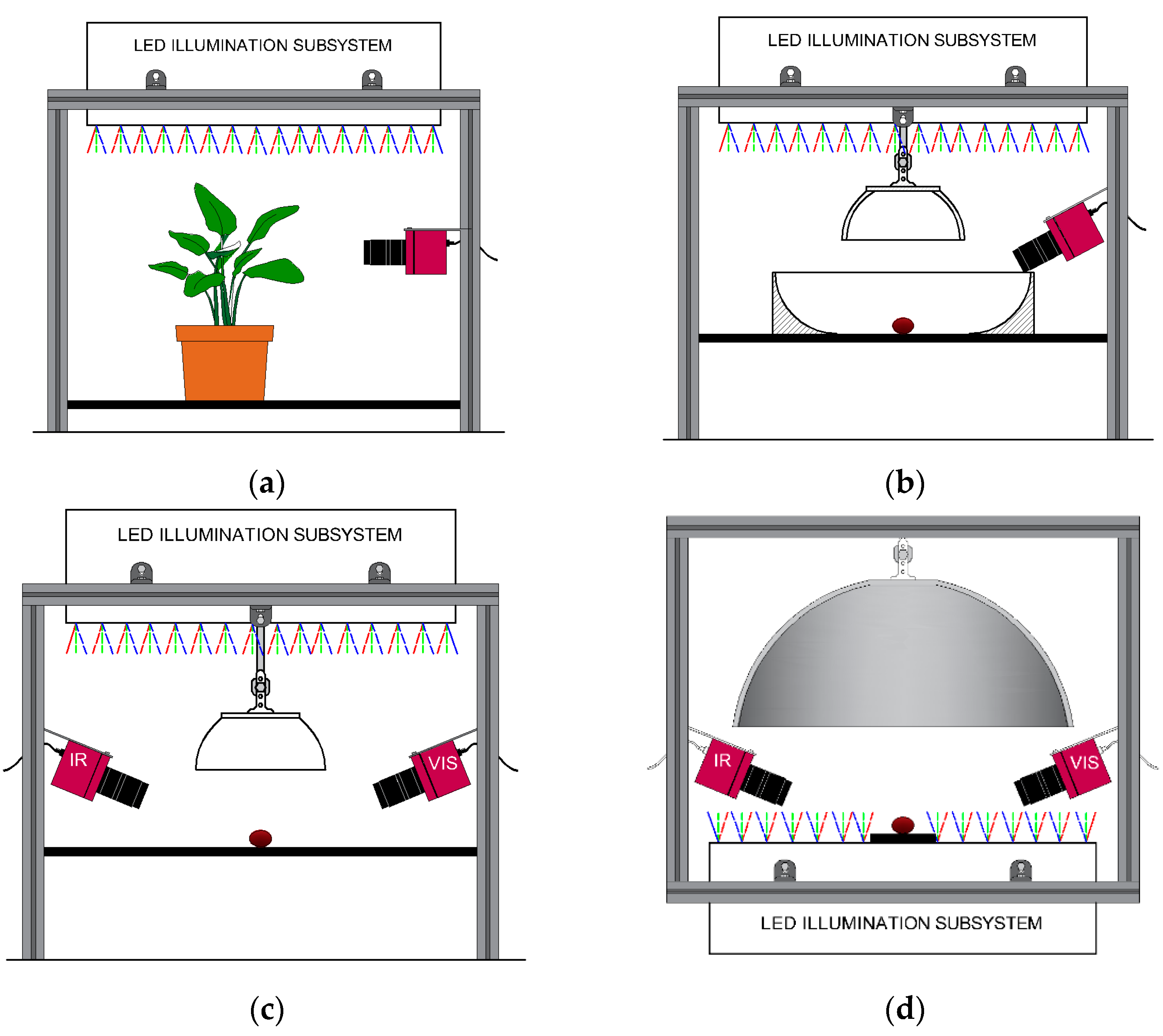
2.1. Multispectral Computer Vision System

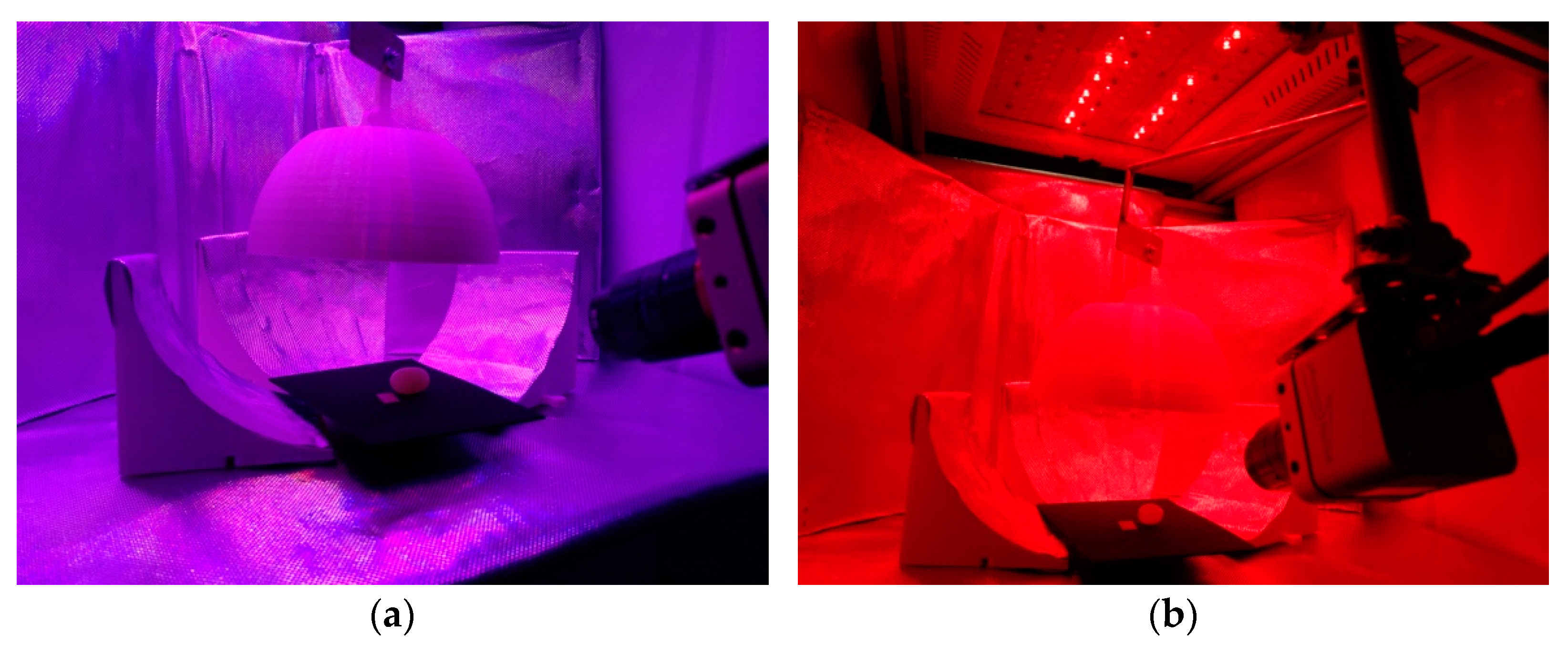
The multispectral computer vision system is composed of (1) a dark chamber, (2) an illumination subsystem, (3) a multispectral image capturing subsystem and (4) a processing subsystem.

2.1.1. Dark Chamber

The dark chamber has a dimension of 1000 × 1000 × 500 mm³ and has been designed to carry out MSI captures of biological systems of different sizes, such as plant organs (flowers, stems or leaves), fruit, vegetables and so on. Depending on the type of object to analyse, the chamber can be configured to avoid undesired reflections, occlusions or shadows. For this reason, it possesses mobile panels, position accessories for cameras and illumination and elements made with a 3D printer, such as domes and semidomes.

Figure 2 shows four configurations of the dark chamber for different experiments: Figure 2a shows direct illumination to capture an MSI for growth analysis of petunia leaves [24]; Figure 2b allows images to be captured with direct illumination with a dome to avoid the reflection of the illumination subsystem on the grape skin and a semidome to eliminate shadows; Figure 2c shows a direct illumination configuration for the simultaneous visible and IR image capturing, avoiding unwanted brightness; and Figure 2d shows a configuration with back-illumination for the simultaneous visible and IR imaging capture with a big dome to allow for correct light distribution.

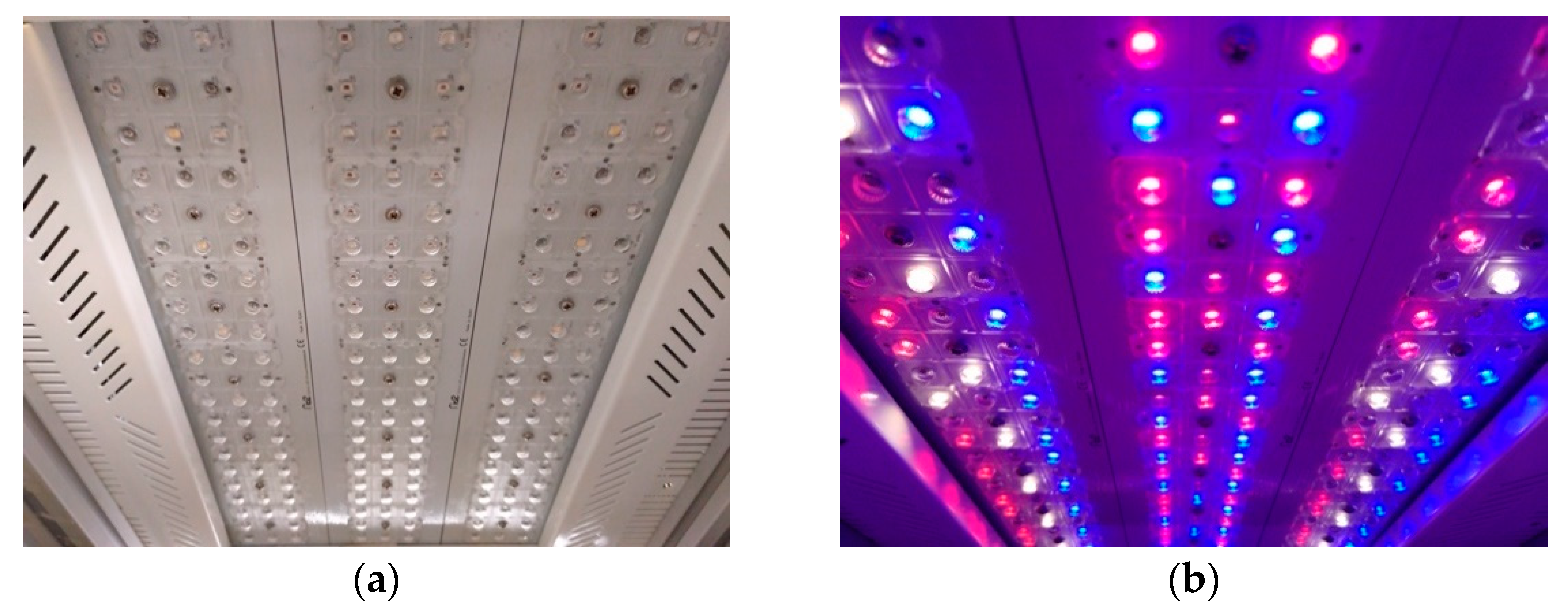
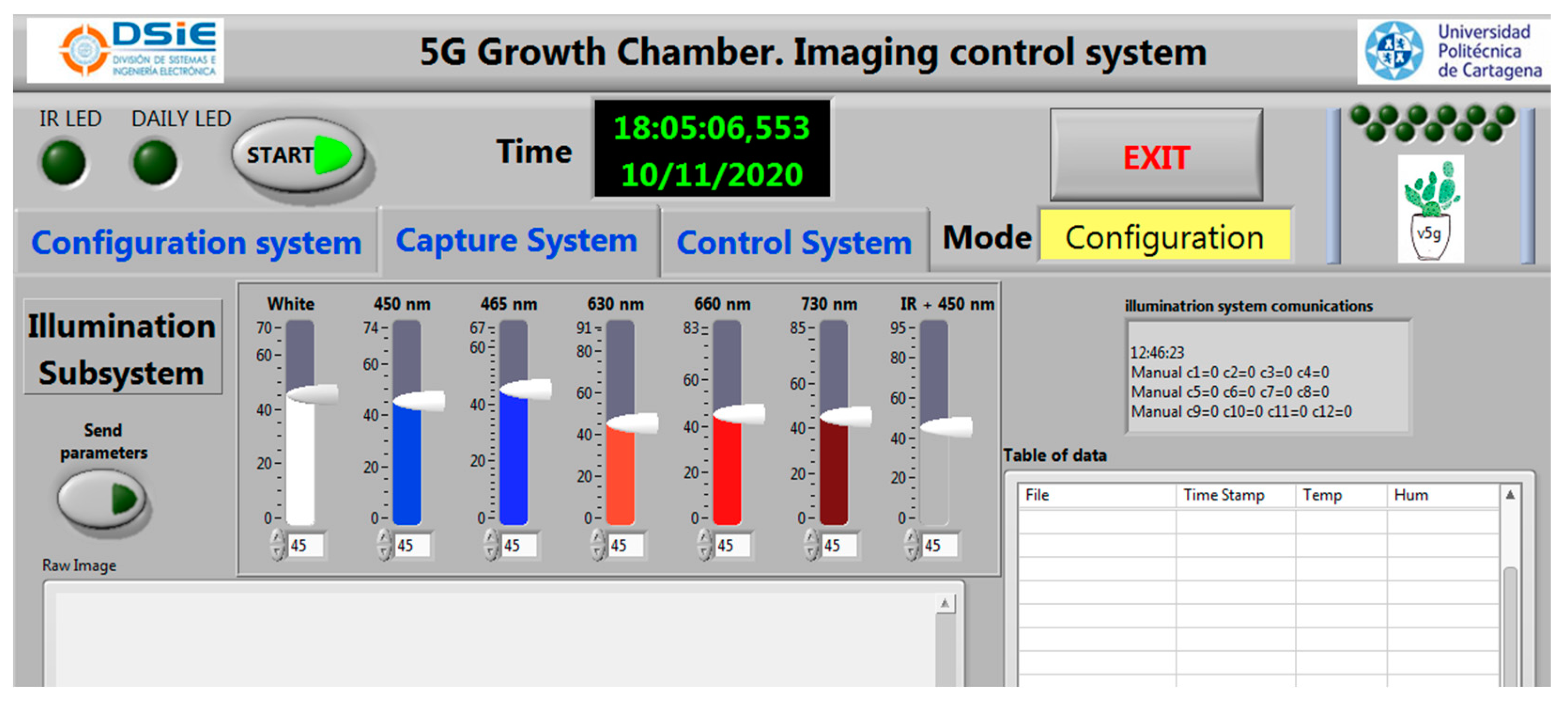
2.1.2. Illumination Subsystem

The illumination subsystem is formed of an electronic module based on a microcontroller capable of managing up to 12 output channels. The module supplies the necessary power to an array of LEDs of different wavelengths, as shown in Figure 3. The power of each channel is configured by means of the lighting control panel of the MSI acquisition subsystem.

The design of the illumination subsystem allows you to add or change the LEDs connected to each channel, as long as they do not exceed the output power of the channel.

Table 1. Channels, spectral range and power per channel.

Channel	C1	C2	C3	C4	C5	C6	C7
Spectra	White	450 nm	465 nm	630 nm	660 nm	730 nm	IR 1
Power	24 W	24 W	24 W	24 W	24 W	24 W	100 W

¹ IR LEDS (760-800-820-840-880-910-940-970) nm.

shows the channel number, the spectra and the power per channel of the illumination subsystem.

2.1.3. MSI Acquisition Subsystem

The main elements of the subsystem consist of two multispectral cameras of mosaic type from Photonfocus: MV1-D2048x1088-HS03-96-G2 [25] and MV1-D2048x1088-HS02-96-G2 [26]. The first camera (HS03) has 16 band-pass filters in the spectral range of 480 nm–630 nm, while the second camera (HS02) has 25 band-pass filters in the spectral range of 600 nm–995 nm. Both cameras can capture up to 41 raw images of 1 byte per pixel in the spectral range of 480 nm–995 nm. After each image capture, a calibration process with two reference images to correct the reflectance values is necessary, as shown in Equation (1):

$$I_{cal}=\frac{I_{raw}\left(t_1\right)-I_{dark}\left(t_1\right)}{I_{white}\left(t_2\right)-I_{dark}\left(t_2\right)}$$

(1)

where $I_{raw}$ and $I_{white}$ are two multispectral images captured with a specific configuration of the illumination subsystem over the object to study and over a white reference surface, respectively; $I_{dark}$ is a multispectral image captured over a black surface in the same illumination conditions; and finally, $t_1$ and $t_2$ refer to two different exposure times used for capturing the image.

To manage and control the MSI acquisition subsystem, a friendly and easy-to-use user interface programmed using LabVIEW on a host computer has been developed, which allows (see Figure 4) one (1) to set the parameters of the multispectral cameras and to obtain calibrated images; (2) to configure the output power of the illumination subsystem (for that, a UDP communication protocol between the host computer and illumination subsystem has been developed); (3) to carry out experiments based on a temporal schedule triggering the multispectral cameras and illumination subsystem; and (4) to log the events of the experiment and handle errors.

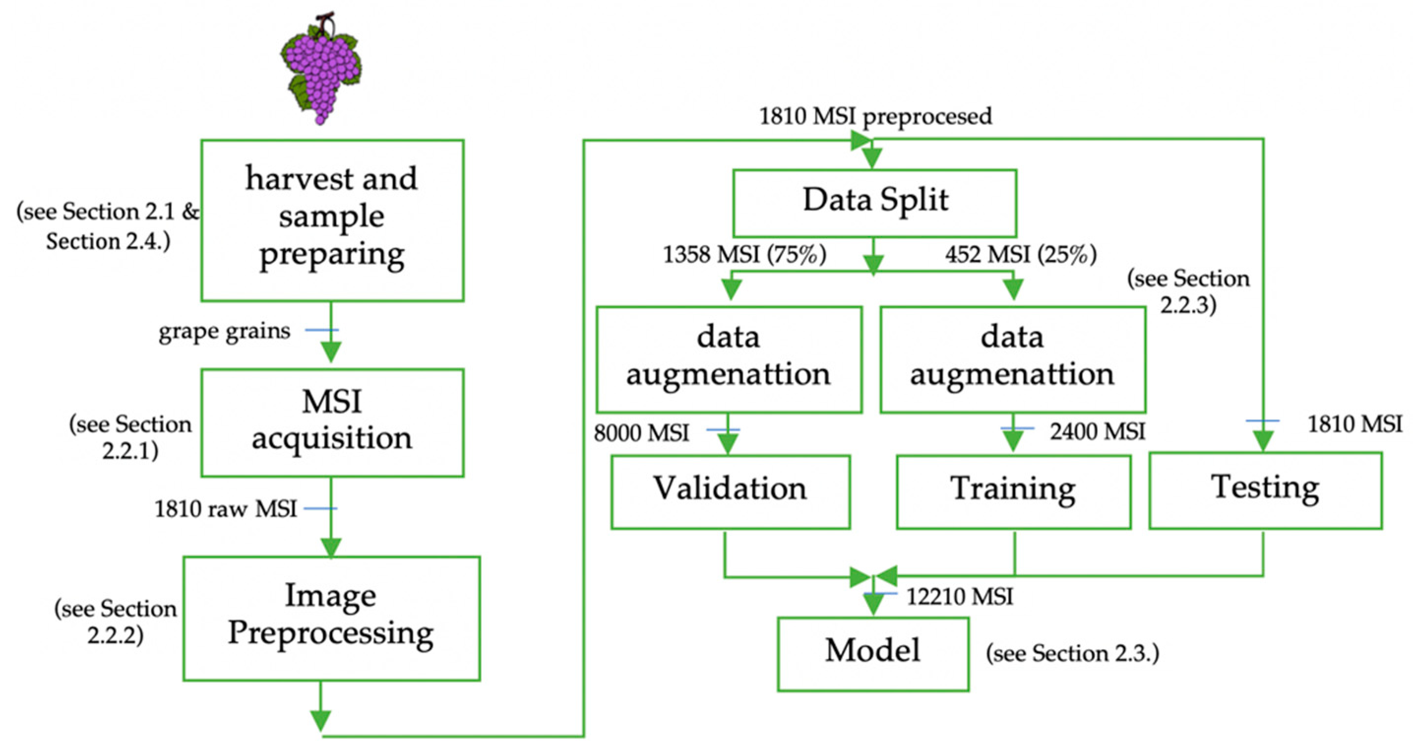
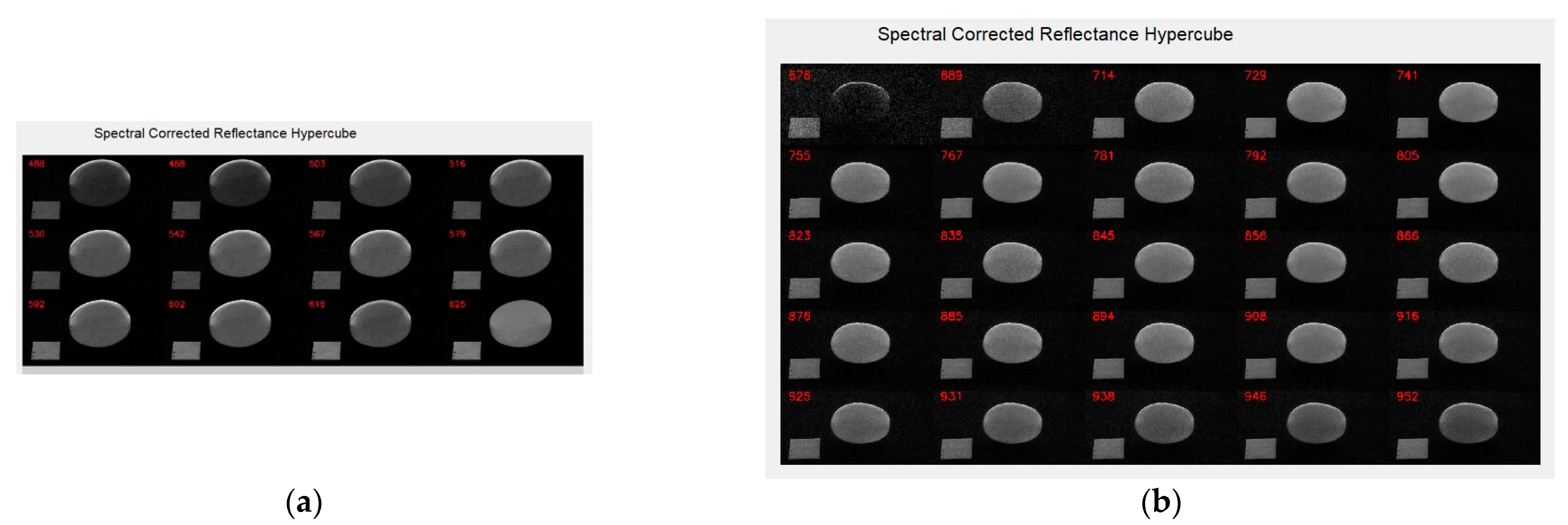
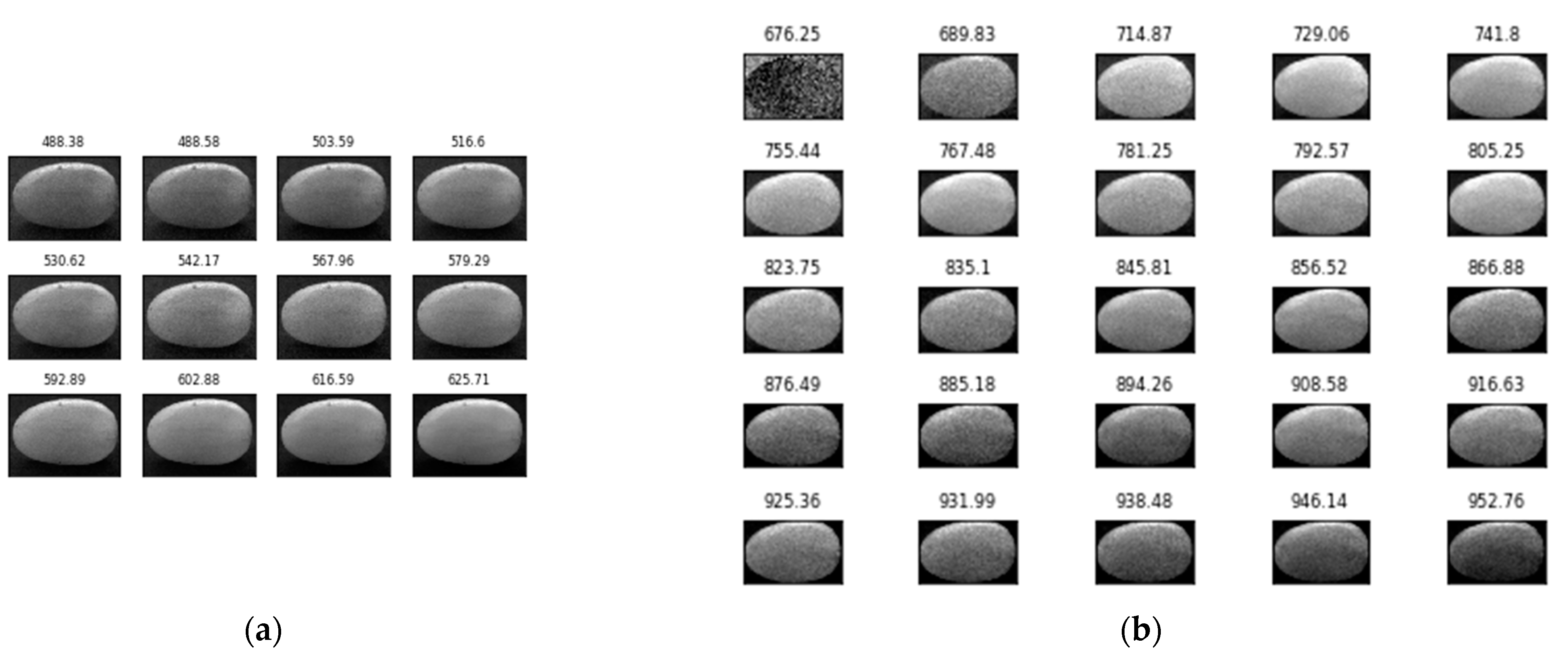
2.2. MSI Acquisition Process and Image Pre-Processing

2.2.1. MSI Acquisition Process

In the multispectral image acquisition process, 1810 berries of five varieties of seedless table grape have been used: 408 grains of Autumn Royal, 602 grains of Crimson Seedless, 196 grains of Itum4, 408 grains Itum5 and 196 grains of Itum9. Figure 5 shows an example of the appearance of a bunch of each variety and an example of the samples used in the vision system. The five varieties used show three colours. Autumn Royal is dark red, Crimson Seedless and Itum9 are red and Itum4 and Itum5 are green. To the human eye, Autumn Royal is clearly darker than the rest. However, it is very difficult to discriminate between Crimson Seedless and Itum9 and between Itum4 and Itum5.

Each grape grain was photographed with the VIS and IR cameras shown in Section 2.1.2. The VIS camera was configured to capture 12 bands that correspond to the spectral wavelengths in nanometres: 488.38, 488.58, 503.59, 516.60, 530.62, 542.17, 567.96, 579.29, 592.89, 602.88, 616.59 and 625.71. The IR camera was configured to capture 25 bands that correspond to the spectral wavelength in nanometres: 676.25, 689.83, 714.87, 729.06, 741.80, 755.44, 767.48, 781.25, 792.57, 805.25, 823.75, 835.10, 845.81, 856.52, 866.88, 876.49, 885.18, 894.26, 908.58, 916.63, 925.36, 931.99, 938.48, 946.14 and 952.76.

Figure 6a,b show the capturing process for the VIS and IR cameras used in the dark chamber. A white reference marker of known dimensions is used in each image for future exact measurements of shape and dimensional calibration.

Figure 7a,b show the 12 VIS images and 25 IR images, respectively, calibrated using Equation (1) for the grape variety Itum5.

2.2.2. Image Pre-Processing

The images captured in the image acquisition process have been pre-processed before being supplied to the Deep Neural Network (DNN) algorithms. The aim of this stage is to separate the image of the grape grain from the background to obtain the most precise spectral information possible, without noise or elements in the image other than the grape. To achieve this, an automatic segmentation algorithm was developed that searches all of the bands in an MSI for the object that most closely resembles a grape using shape characteristics. Then the region that contains the grape is used to extract the grapes from all the bands. The algorithm developed is made up of a processing pipeline of basic computer vision methods, which are described below:

• Load an MSI consisting of N bands: MSI = {B₀,…,B_N}.
• Calculate the mean Shannon entropy for all the bands of the MSI (MSE), as well as for each band: {SE₀,…,SE_N}.
• For each entropy value SE_i:
  • If MSE > SE_i, we consider that the image has an acceptable information distribution and the Otsu [27] thresholding method will be applied, obtaining a new set of black-and-white images {BW₀,…,BW_N}.
  • Otherwise, we consider that the image has a low information distribution, and the bands will be limited with a threshold value of 10, obtaining a new set of black-and-white images {BW₀,…,BW_N}.
  • A contour search algorithm will be applied to the images {BW₀,…,BW_N}, obtaining a new set of contours {C₀,…,C_M}. From the set, those contours {C₀,…,C_K} that verify the area and roundness restriction criteria given by Equation (2) will be selected:

    $$C_j\in \left\{C_0,\dots C_K\right\} if \{\begin{array}{c}8000<\mathrm{area}\left(C_j\right)<40000)\\ \bigwedge \\ 0.4<\mathrm{circularity}\left(C_j\right)<1.2)\end{array}$$

    (2)
• From the set of contours {C₀,…,C_j,…,C_M}, which verify the area and roundness restrictions, the one with the largest area, C_m, will be selected as the best segmentation of the grape. The window containing the contour C_m(y:y+h,x:x+w) will be used to segment all of the grapes of each band of the MSI, where (y,x) is the upper-left corner of the rectangle, h the height and w the width.
• Each MSI has been resized to a size of 140 × 200 pixels.
• Go to step 1.

Figure 8a,b show the result of the pre-processing applied to a visible MSI and an MSI captured in IR, respectively.

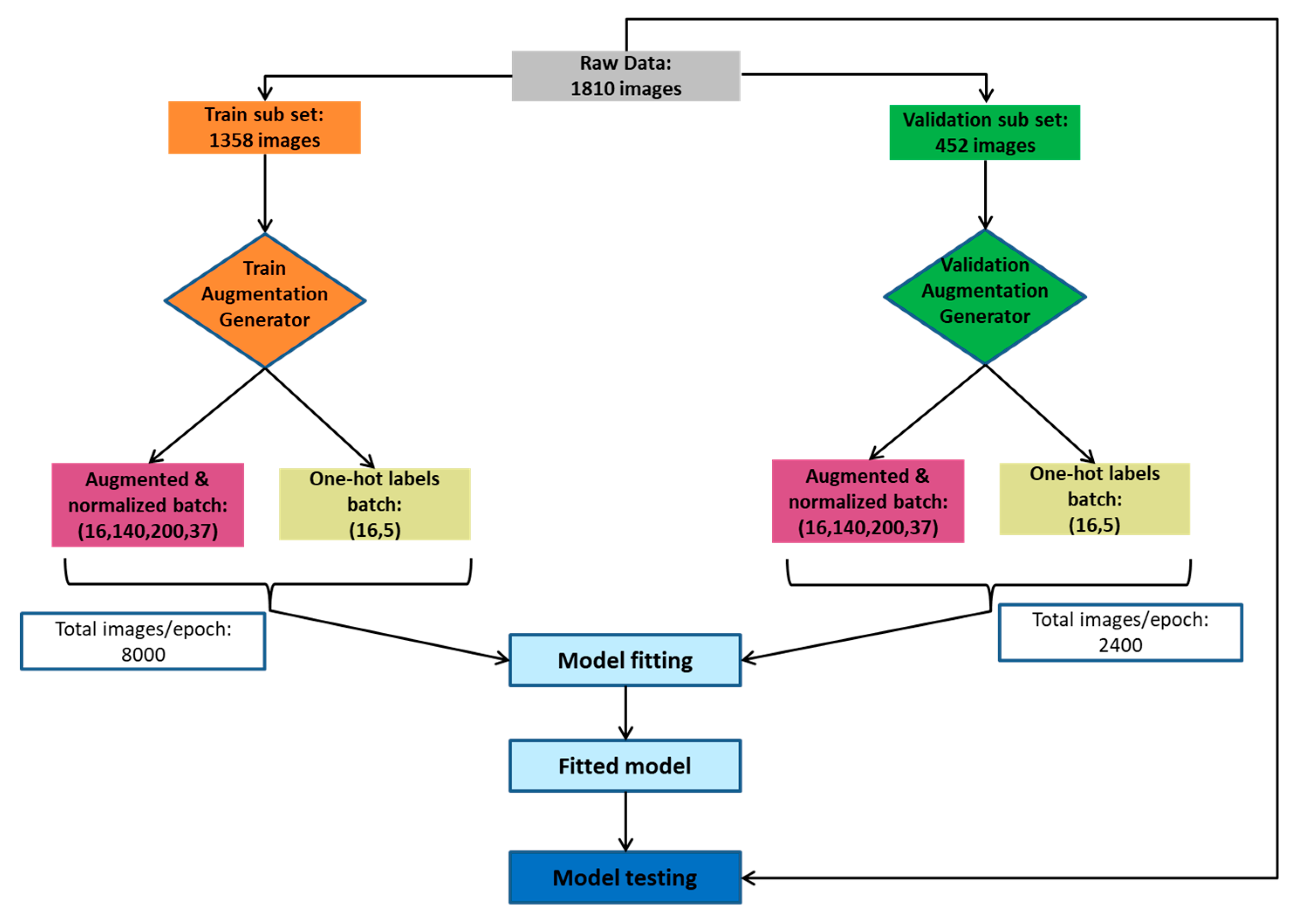
2.2.3. Data Augmentation

The original dataset was split into training and validation subsets of 1358 and 452 images, that account for 75% and 25% of the images, respectively. The class distribution in both subsets is the same, as the test subset contains 25% of the images of each of the five different grape varieties used.

To increase the number of training images, a data augmentation pipeline was developed using the Python library API, Albumentations [28]. The new augmented images were generated by sequentially applying the following transformations with a set probability of 50% each: either horizontal or vertical flip, random contrast and brightness alteration, and affine transformation. This last one includes horizontal and vertical shifts, rotation and scaling of the images. All the transformations were controlled with parameter values selected randomly within a defined range, except for the horizontal and vertical flip (

Table 2. Transformation ranges of data augmentation.

Transformation	Range
Brightness	(−0.15,+0.15)
Contrast	(−0.15,+0.15)
Rotation	(−90,+90°)
X axis shift	(−0.006,+0.006)
Y axis shift	(−0.006,+0.006)
Scale	(−0.3,+0.3)

).

The data augmentation pipeline was implemented in a generator-type Python function, and therefore, the new data were not stored but generated in fixed-size batches in each training step of the classification models (see Figure 9). The function randomly selects a number of images from the training subset equal to the batch size and then applies the augmentation pipeline described earlier to every image. After a batch of augmented images is created and before it is delivered to the training algorithm, it is normalised to a range of pixel values from 0 to 1, by dividing by 255 the maximum possible value in 1-byte resolution images.

The test and training datasets were augmented with the same augmentation pipeline. As the data are already separated into two subsets before being fed to the generators, there is no risk that the test generator will produce images equal or very similar to the ones that have been generated by the training generator, which could lead to lower loss values in the test dataset and erroneous conclusions about the performance of the models. The class distributions of both augmented datasets are the same because of the random selection of images to transform from the dataset and, as mentioned earlier, the subsets have been created respecting the class distribution.

The total number of images generated in any training epoch is equal to the batch size, 16 times the number of steps per epoch, which were 500 for the training phase and 150 for the validation, making a total of 8000 images for training and 2400 for validating. Finally, after fitting, each model was tested using the 1810 original images without any augmentation.

The following diagram illustrates the whole process.

2.3. Deep Learning Methods

Methods based on deep learning belong to the group of algorithms associated with machine learning and have proven their effectiveness in various fields of science; in addition there is a growing interest from the scientific and research communities. Among the most used methods are (1) convolutional neural networks (CNNs), (2) recurrent neural networks (RNNs), (3) generative adversarial networks, (4) Boltzmann machines, (5) deep reinforcement and (6) autoencoders.

In this work, we used CNNs as the tool to perform the multispectral image classification of five varieties of grape grains. CNNs were designed to avoid the tedious feature extraction processes that computer vision experts previously used to carry out the segmentation and classification of objects in images. CNNs have the capacity to automatically extract the most relevant characteristics that minimise a certain function, $f^{\ast }$. The goal of the CNN classification model $y=f^{\ast }\left(x\right)$ is to map an input $x$ to a category $y$. The network is capable of learning a set of parameters, $\theta$, that obtain the best function approximation $y=f^{\ast }\left(x;\theta \right)$ [29].

At the architecture level, CNNs are composed of different layers (L), which are grouped into blocks that can be distributed into different branches and unions. Figure 10 shows some of the most common blocks used to create CNN architectures. The advantages of these architectures are that once trained, they can be reused for different applications.

To solve a certain classification problem, the blocks shown in Figure 10 are selected and assembled with the aim of forming an architecture that can optimise the mapping of input images in one or more output classes. The most used layers in these blocks that form the CNN architectures are described below:

• Input layer. This is the data input layer of the CNN and is composed of the normalised training images. These images can have a single channel or multiple channels, such as multispectral, video or medical images (i.e., magnetic resonance imaging (MRI) and computerised tomography (CT) scans).
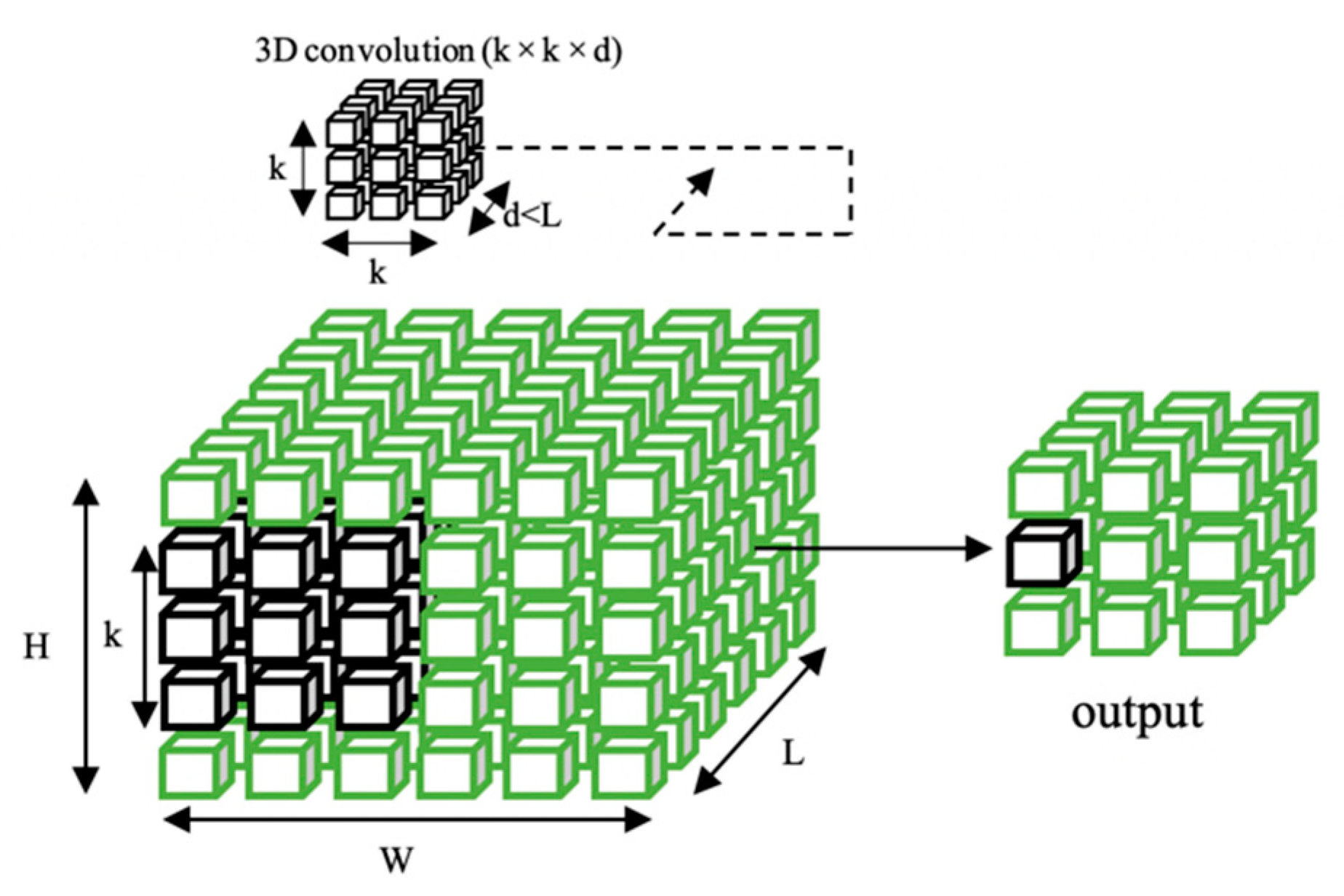
• Convolutional layers. These units have the ability to extract the most relevant characteristics from the images. The convolutions on the images are usually 2D. Given an image I and a convolution kernel K, the 2D convolution operation is defined by Equation (3).

  $$\mathrm{S}\left(\mathrm{i},\mathrm{j}\right)=\left(\mathrm{I}\ast \mathrm{K}\right)\left(\mathrm{i},\mathrm{j}\right)={\displaystyle \sum }_m{\displaystyle \sum }_{n}I\left(m,n\right)K\left(i-m,j-n\right)$$

  (3)

Equation (3) allows the extraction of spatial features from images in 2D. However, there are other convolutions that exploit the multidimensional relations present in images with either 2 or 3 dimensions. These are called 3D convolutions [30], and the main difference compared to the 2D convolutions is that the kernel used has 3 dimensions instead of 2. This can be imagined as a data cube (k × k × d), which would be the filter that moves along the 3 spatial axes of an image with a given stride and performs the dot product between the pixel values of the image and the numbers in the filter, at each step, as can be seen in Figure 11.

To apply a 3D convolution to a 2D image of size W × H × L (width pixels times height pixels times the number of channels), the array that constitutes the image must be reshaped so that the channel axis is interpreted as a third depth axis, and a fourth axis of size 1 is added, which would be the channel axis of a proper 3D image that contains the pixel values. In the case of a normal 2D image defined with the common RGB colour map, there is likely little to gain by applying 3D convolutions, because the channel axis is only of depth 3, and as such, there is not much information stored in it compared to the spatial axes of larger sizes. Thus, the channel axis is larger and contains more information about the object being captured than the channel axis of an RGB image, namely the reflectance at various wavelengths. Therefore, in this case, applying 3D convolutions can lead to better results with a deep learning model using fewer convolutional layers and, in turn, fewer parameters.

• Fully connected layers. These layers are those layers where all the inputs from one layer are connected to every unit of the next layer. They have the capacity to make decisions, and in our architecture, they will carry out the classification of the data into various classes.
• Activation layer. It has the capacity to apply a nonlinear function as output of the neurons [31]. The most commonly used activation function is the rectified linear unit (ReLU), and it is defined in Equation (4).

  $$ReLU\left(x\right)=\{\begin{array}{c}x, x\ge 0\\ 0, x<0\end{array}$$

  (4)
• Batch normalisation layer. This layer standardises the mean and variance of each unit in order to stabilise learning, reducing the number of training epochs required to train deep networks [29].
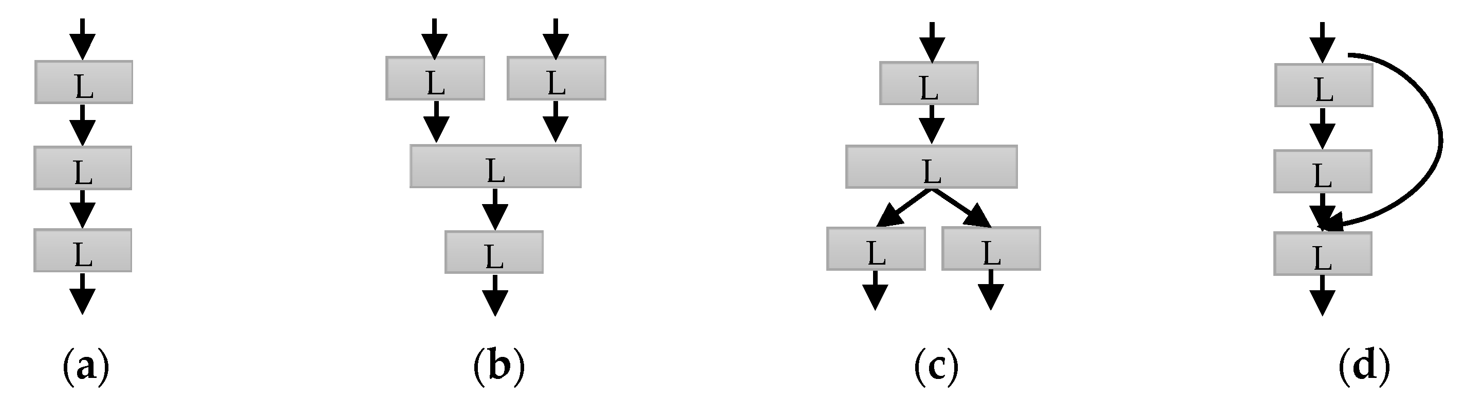
• Pooling layer. The pooling layer modifies the output of the network at a certain location with a summary statistic of the nearby outputs, and it produces a down-sampling operation over the network parameters. For example, the Max Pooling layer uses the maximum value from each of the clusters of neurons at the prior layer [32]. Another common pooling operation is the calculation of the mean value of each possible cluster of values of the tensor of the previous layer, which is implemented in the Average Pooling layer. Both of these kinds of pooling operations can be applied to the whole tensor of the prior layer instead of just a cluster of its values in a sliding window that moves along it. These layers are called Global Max Pooling and Global Average Pooling, and they reduce a tensor to its maximum or mean value, respectively. Additionally, every pooling operation can be applied two- or three-dimensionally, which means that they act along the first 2 or 3 axes of the given tensor. For instance, a 3D Global Average Pooling layer would reduce a tensor of size w × h × d × f (width times height times depth times features) to a 1 × f one, thus spatially compressing the information of every feature to just one value, its mean.
• Output layer. In CNNs for classification, this layer is formed by the last layer of the fully connected block and contains the activation layer, which obtains the probability of belonging to a particular class.

2.3.1. Pretrained DL Architectures

Over the course of the last decades, there have been many advances in the design of CNN architectures, which have been increasing in depth and complexity, allowing for impressive results in many deep learning projects. Some of the most well-known architectures include LeNet-5, AlexNet, VGG16, ResNet and the Inception variants, which will be briefly reviewed below.

• LeNet-5 was published in 1998 and was originally conceived to recognise handwritten digits in banking documents. It is one of the first widely used CNN and has served as the foundation for many of the more recently developed architectures. The original design consisted of two 2D convolution layers with a kernel size of 5 × 5, each one followed by an average pooling layer, after which a flattening layer and 3 dense layers were placed, the last one being the output layer. It did not make use of batch normalisation and the activation layer was tanh instead of the now widely used ReLU [33].
• AlexNet was published in 2012 and won the contest of ImageNet LSVRC-2010, which consisted of the classification of 1.2 million images of 1000 distinct classes. The network has a significantly larger number of parameters compared to LeNet-5, about 60 million. It consists of a total of five 2D convolutional layers, of varying kernel size that decrease with the depth of the layer: 11 × 11, 5 × 5 and 3 × 3 for the last 3. In between the first three convolutional layers and after the last one, there are a total of 4 Max Pooling layers. Then, a flattening layer and three dense layers follow, including the final output layer. The innovations of this CNN are the usage of the ReLU activation function and the dropout layers to reduce overfitting. Also, the usage of GPUs to train any CNN model with more than a million parameters, which is now commonplace, can be traced back to the inception of this architecture [34].
• VGG16 was published in 2014 as a result of the investigation of the effect of the kernel size on the results achieved with a deep learning model. It was found that with small kernel sizes of 3 × 3 but an increased number of convolutional layers, 16 in this case, the performance experienced a significant improvement. This architecture won the ImageNet challenge of 2014 and consists of 16 convolutional layers, all with kernel size 3 × 3, grouped in blocks of two or three layers each. The groups are followed by Max Pooling layers, and after the last convolution block, there are three dense layers, including the output layer. This architecture showed that the deeper the CNN is, the better the results achieved by it usually are, but the memory requirements also increase and must be taken into account. The number of parameters of this architecture is very high, 137 million, but the authors created an even deeper network, called VGG19, with 144 million parameters [35].
• Inception was published in 2014 and competed with VGG16 in the same ImageNet challenge, where it achieved results as impressive as those of VGG16 but using far less parameters, only 5 million. To accomplish this, the architecture makes use of the so-called inception blocks, which consist of 4 convolutions applied in a parallel manner to the input of the block, each one of a different kernel size, and whose outputs are, in turn, concatenated. The network is made of 3 stacked convolutional layers and then 9 Inception blocks, followed by the output layer. There are also 2 so-called auxiliary classifiers that emerge from 2 Inception blocks, whose purpose is to mitigate the vanishing gradient problem that accompanies a large neuronal network like this. These two branches are discarded at inference time, being used only during training. The kernel sizes of all the convolutional layers were chosen by the authors to optimise the computational resources. After this architecture was published, the authors designed improved versions like InceptionV3 in 2015 and Inception V4 in 2016. InceptionV3 focused on improving the computation efficiency and elimination of representational bottlenecks [36], and InceptionV4 took some inspiration from the ResNet architecture and combined its residual connections, which will be briefly discussed below, with the core ideas of InceptionV3 [37]. In 2016, yet another variant of Inception was published, called Xception. Its main feature is the replacement of all the convolutions by depth-wise separable convolutions to increase the efficiency even further [38].
• ResNet was published in 2015 and won the first place of the ILSVRC classification task of the year. The main new feature of this architecture are the skip connections and the consistent usage of batch normalisation layers after every convolutional layer. The purpose of these features is to ease the training of very deep CNNs, like the implementations ResNet-50 and ResNet-101, which have 50 and 101 convolutional layers, respectively. The architecture is composed of so-called convolutional and identity blocks, in which the input to the block is concatenated to its output, creating the skip connections that help to train the networks [39].

All of these architectures have been used in the field of remote sensing in numerous studies. In the case of LeNet-5, for example, in [40], the authors used a slightly modified version of this CNN, among others, to track the eyes of typhoons with satellite IR imaging; and in [41], they created, as part of their study, a pretrained LeNet-5 model using the UC Merced Dataset to classify cropland images. AlexNet is used in [42] to classify the images of the UCM spaceflight, dataset and in [43], a pretrained AlexNet model is fine-tuned to classify wetland images. VGG16 and 19, InceptionV3, Xception and ResNet50, among others, are used in a comparative study [44] to classify complex multispectral optical imagery of wetlands. In [45], the authors designed an improved version of InceptionV3 to classify ship imagery from optical remote sensors. This architecture is also the base of the one used in [46] to classify images of damaged buildings by earthquakes using high-resolution remote sensing images; and in [47], the authors pretrained an ImageNet2015 InceptionV3 model together with VGG19 and ResNet50 to classify images of high spatial resolution. The Xception architecture was used in [48] to detect palm oil plantations, and ResNet50 was used in [49] to detect airports in large remote sensing images. These are just a few examples of the many existing studies in which CNN algorithms are used.

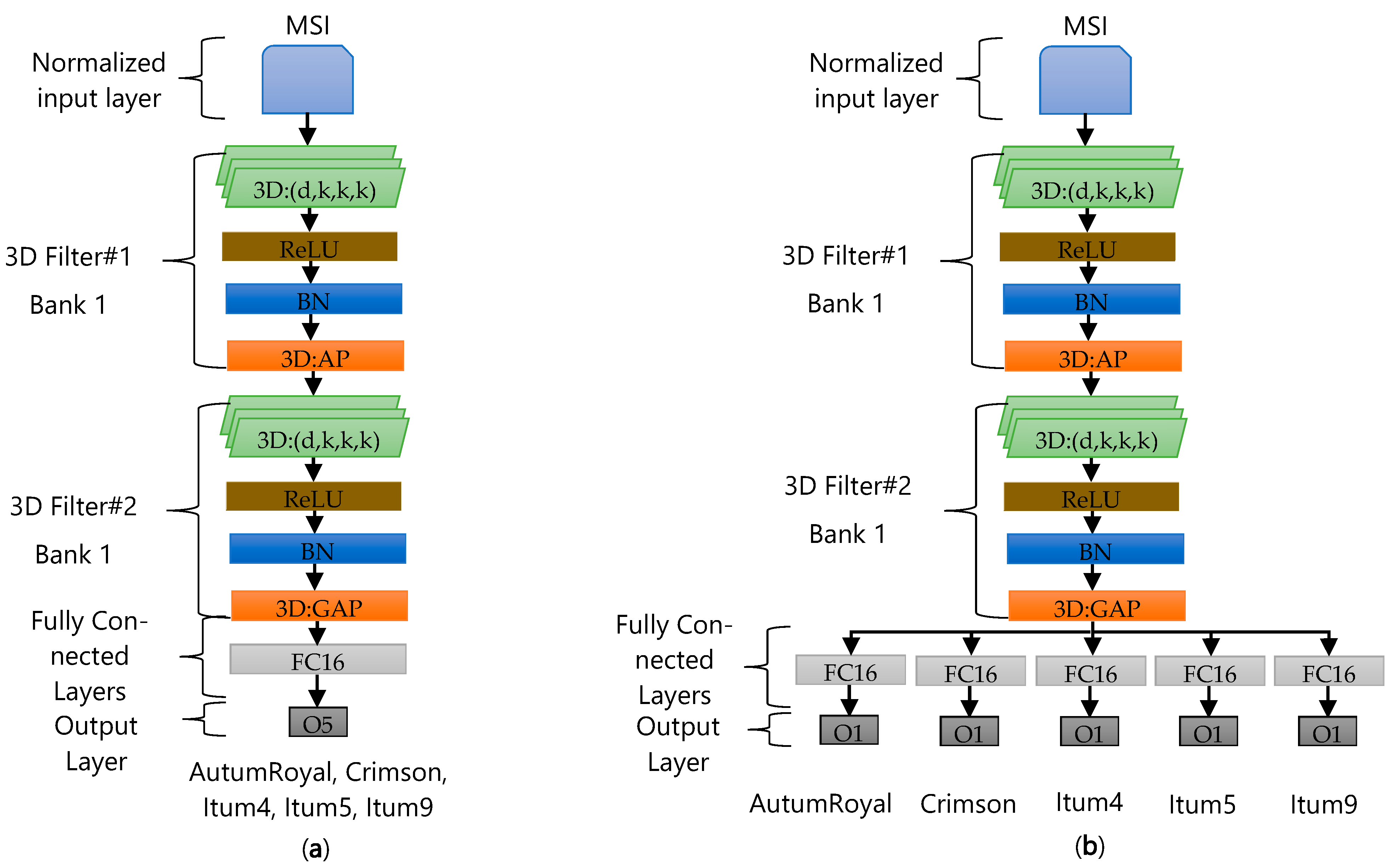
2.3.2. Ad hoc Deep Learning Architecture Design

To perform the classification of the five grape varieties, two custom architectures have been designed, consisting of the following layers: (1) a normalised input layer; (2) two 3D filter blocks made up of 3D convolutional layers (3D:d,k,k,k), a ReLU activation function, Bath normalisation and 3D Pooling layers (Filter#1: 3DAveragePooling (3D:AP); Filter#2: 3D GlobalAveragePolling (3D:GAP)); (3) a fully connected (FC) layer; and (4) an output (O) layer. The first architecture (Figure 12a) is formed by a sequential structure of layers with a single-branch output (SBO), while the second proposed architecture is similar to the first (Figure 12b) but has an output distributed as a multiple-branch output (MBO). Both architectures have been designed to exploit the multidimensionality present in multispectral images, for which a 3D filter block has been designed consisting of four layers (see Figure 12a,b), which has allowed the extraction of spatial-spectral features of the different bands captured by the vision system to be maximised.

With the aim of obtaining an optimal design for the parameters of the SBO and MBO architectures regarding the 3D filter banks, two types of test have been designed:

(1)

Optimal 3D kernel size. In this test, both architectures were evaluated with symmetric kernel sizes: (5 × 5 × 5), (7 × 7 × 7) and (10 × 10 × 10). The different kernels will allow different space–time relationships to be captured for the multispectral images and the evaluation of the size that produces the best result in the classification process.

(2)

Optimal kernel sequence: In this experiment, architectures with three types of kernel sequences were evaluated: increasing F#1(5 × 5 × 5) + F#2(10 × 10 × 10), decreasing F#1(10 × 10 × 10) + F#2(5 × 5 × 5) and constant F#1(7 × 7 × 7) + F#2(7 × 7 × 7). The results will allow the influence of the sequence order of the kernels on the classification process to be determined.

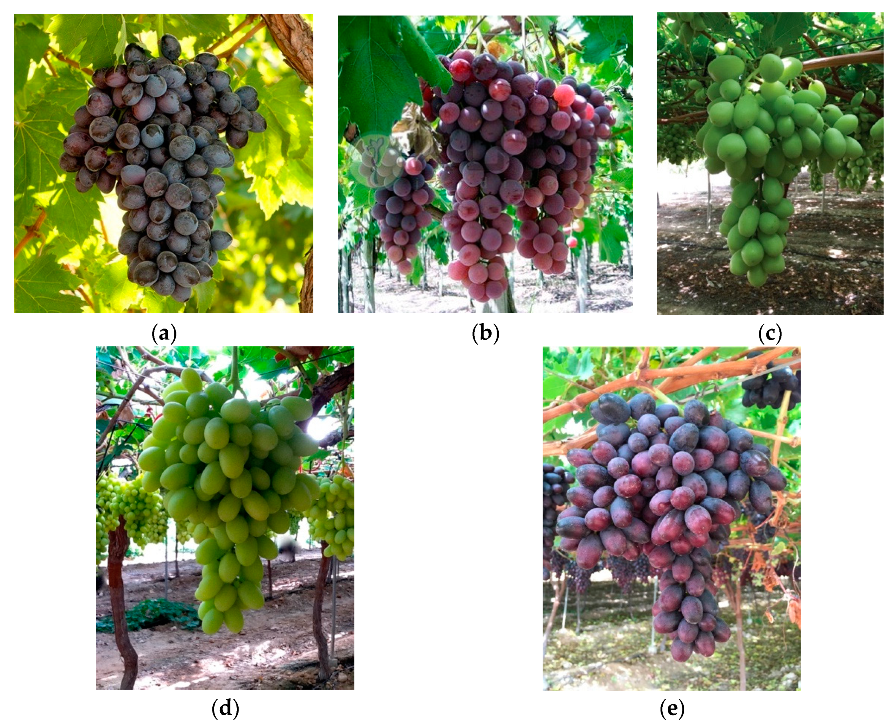
Both tests have been performed with a kernel depth of d = 16 and have used a dilation rate of 2 × 2 × 2 in the 3D convolutional layer.

Table 3. Number of parameters per layer and total of SBO and MBO architectures.

	Architecture Layer	SBO (5 × 5 × 5) [(0 × 10 × 10)	SBO (10 × 10 × 10) (5 × 5 × 5)	SBO (7 × 7 × 7) (7 × 7 × 7)	MBO (5 × 5 × 5) (10 × 10 × 10)	MBO (10 × 10 × 10) (5 × 5 × 5)	MBO (7 × 7 × 7) (7 × 7 × 7)
	Input	0	0	0	0	0	0
Filter#1	3D:Conv	1008	8008	2752	1008	8008	2752
	ReLU	0	0	0	0	0	0
	BN	32	32	32	32	32	32
	3D:MP	0	0	0	0	0	0
Filter#2	3D:Conv	128,016	16,016	43,920	128,016	16,016	43,920
	ReLU	0	0	0	0	0	0
	BN	64	64	64	64	64	64
	3D:GAP	0	0	0	0	0	0
	FC16	272	272	272	1360 1	1360 1	1360 1
	Output	85	85	85	85 2	85 2	85 2
Total Parameters		129,477	24,477	47,125	130,565	25,565	48,213

¹ Five FC16 branches: 272 × 5 = 1360. ² Five outputs: 17 × 5 = 85.

shows the total number parameters for each architecture and per layer that have been used after configuring the architectures in Figure 12 according to the tests designed for calculating the optimal number of parameters.

2.4. Plant Material

All grape varieties used in the current study were grown in a commercial orchard (Cooperativa Las Cabezuelas), where seedless grapes and Narcissus are grown for export under ecological conditions [50]. Seedless grapes are of the commercial varieties Crimson Seedless, Autumn Royal, Itum4, Itum5 and Itum9. While Crimson Seedless and Autumn Royal are classic seedless grapes, the Itum series correspond to a new selection created recently for high-quality table grapes [51]. All seedless grapes share a common mutation rendering stenospermocarpic seed abortion [52]. Grapes were harvested when ready to market. Starting in mid-June and till late December, different varieties were transported to the lab and conserved in a cold chamber at 6° during the image acquisition period.

3. Results

In the design and implementation phase of the deep learning architectures for the classification of multispectral images, the Keras 2.3.1 under TensorFlow 2.0.0 libraries have been used. The Albumentation library [28] has been used in the data augmentation process for multichannel images, and the OpenCV library [53] has been used in the implementation of the image pre-processing algorithm (Section 2.2.2). The methods proposed were programmed in Python 3.0 with the Spyder 3.0 IDE running on a computer installed with Windows 10 Professional with Intel Core™ processor i7-7700K at 4.20 GHz, 64 GB DDR4 and dedicated graphics NVIDIA GeForce 1080 with 8 GB memory.

3.1. Configuration of the Models

Three multispectral datasets were used for obtaining the classification models of the five grape varieties with each of the configurations proposed for each architecture.

(1)

Training dataset, which consists of 8000 images, 75% of the images obtained in the data augmentation process (Section 2.2.2)

(2)

Validation dataset, consisting of 2400 images, which corresponds to 25% of the images obtained in the data augmentation process (Section 2.2.2)

(3)

Test dataset, made up of 1810 images, which constitute the set of images without the initial data augmentation

Table 4. Hyperparameter configuration.

Parameter Name	Value
Batch size	16
Number of epochs	20
Optimisation algorithm	Adam
Loss function	Categorical cross Entropy
Metric	Accuracy
Learning rate	0.001
Momentum	None
Activation function in convolutional layers	ReLU
Activation function in last layers	Softmax

shows the hyperparameters used to configure the training and validation phases of all the classification models developed in this work.

3.2. Performance Metrics

To evaluate the performance of the proposed architectures, the metrics accuracy in percentage and the loss function error were calculated during the training and validation of the models. The accuracy in percentage was used to evaluate the test dataset. In addition, the confusion matrix was calculated to obtain more precise information about the classification process of the grape varieties.

Table 5. Training, validation and test accuracy and loss function error for three different filter sequences of SBO and MBO architectures.

Architecture	SBO Kernel Sizes			MBO Kernel Sizes
Metrics	(5 × 5 × 5) (10 × 10 × 10)	(10 × 10 × 10) (5 × 5 × 5)	(7 × 7 × 7) (7 × 7 × 7)	(5 × 5 × 5) (10 × 10 × 10)	(10 × 10 × 10) (5 × 5 × 5)	(7 × 7 × 7) (7 × 7 × 7)
Train. acc. {%)	100.00	100.00	100.00	100.00	99.89	100.00
Train. loss	0.00072	0.0063	0.00030	0.00035	0.01379	0.00069
Val. acc. (%) Epoch	100.00 11	82.708 14	100.00 7	100.00 10	100.00 13	100.00 15
Val. loss	0.00202	0.583	3.693 × 10−5	0.00012	0.00018	0.00025
Test acc. (%)	100.00	83.20	100.00	100.00	100.0	100.00

shows the accuracy and loss values of the different tests performed with the datasets (training, validation and test) used for training, validation and testing of the models for each of the settings in the filter banks ((5 × 5 × 5) + (10 × 10 × 10), (10 × 10 × 10)+ (5 × 5 × 5) and (7 × 7 × 7) + (7 × 7 × 7)) established in the SBO and MBO architectures.

The results shown in Table 5 confirm that the designs proposed for the SBO and MBO architectures based on two 3D filter blocks managed to classify 100% of the grape berries correctly. With the validation and testing sets, a rating of 100% was obtained with all the proposed architectures except with the SBO architecture and kernel sizes: F#1(10 × 10 × 10) + F#2(5 × 5 × 5).

As for the relationship between the distribution of kernel sizes in 3D filter blocks and the number of epochs, it should be noted that the constant kernel sequence F#1(7 × 7 × 7) + F#2(7 × 7 × 7) achieved a maximum rating value with only 7 epochs out of a total of 20.

In addition, in Figure 1, it can be observed that the data augmentation process followed in Section 2.2.2 by which a set of 10,400 multispectral images have been generated, starting from a set of 1810 images captured in the dark chamber, allowed models that have been able to generalise and classify all of the original images in the test set to be obtained.

Table 6. Confusion matrix for the three configurations of the 3D convolution layer in the SBO architecture over test data.

3D Conv.	Variety	Autumn Royal	Crimson Seedless	Itum4	Itum5	Itum9
F#1(5 × 5 × 5) F#2(10 × 10 × 10)	Autumn Royal	100%	0	0	0	0
	Crimson	0	100%	0	0	0
	Itum4	0	0	100%	0	0
	Itum5	0	0	0	100%	0
	Itum9	0	0	0	0	100%
F#1(10 × 10 × 10) F#2(5 × 5 × 5)	Autumn Royal	100%	0	0	0	0
	Crimson	34.55%	63.95%	1.33%	0.17%	0
	Itum4	1.02%	0	98.98%	0	0
	Itum5	15.69%	0	0	84.31%	0
	Itum9	10.26%	0	0	0	89.74%
F#1(7 × 7 × 7) F#2(7 × 7 × 7)	Autumn Royal	100%	0	0	0	0
	Crimson	0	100%	0	0	0
	Itum4	0	0	100%	0	0
	Itum5	0	0	0	100%	0
	Itum9	0	0	0	0	100%

and

Table 7. Confusion matrix for the three configurations of the 3D convolution layer in the MBO architecture over test data.

3D Conv.	Variety	Autumn Royal	Crimson Seedless	Itum4	Itum5	Itum9
F#1(5 × 5 × 5) F#2(10 × 10 × 10)	Autumn Royal	100%	0	0	0	0
	Crimson	0	100%	0	0	0
	Itum4	0	0	100%	0	0
	Itum5	0	0	0	100%	0
	Itum9	0	0	0	0	100%
F#1(10 × 10 × 10) F#2(5 × 5 × 5)	Autumn Royal	100%	0	0	0	0
	Crimson	0	100%	0	0	0
	Itum4	0	0	100%	0	0
	Itum5	0	0	0	100%	0
	Itum9	0	0	0	0	100%
F#1(7 × 7 × 7) F#2(7 × 7 × 7)	Autumn Royal	100%	0	0	0	0
	Crimson	0	100%	0	0	0
	Itum4	0	0	100%	0	0
	Itum5	0	0	0	100%	0
	Itum9	0	0	0	0	100%

show the confusion matrices for the test dataset. The results in both tables show that the SBO and MBO architectures do not show any difference when classifying 100% of the five grape varieties with increasing and constant kernel sequences. On the other hand, the decreasing kernel sequence ((10 × 10 × 10) + (5 × 5 × 5)) obtained worse results in the classification for both architectures. The MBO architecture offers a 99.40% correct classification compared to 83.20% for the SBO architecture; specifically, the SBO architecture had the biggest problems classifying the Crimson Seedless, Itum5 and Itum9 varieties.

Finally, and from the values in Table 3, the total number of parameters for each of the configurations of the SBO (129,477, 24,477, 47,125) and MBO (130,565, 25,565, 48,213) architectures do not show significant differences. The architecture with the most parameters is MBO with an increasing kernel sequence F#1(5 × 5 × 5) + F#2(10 × 10 × 10), and that with the least parameters is the SBO with a decreasing kernel sequence F#1(10 × 10 × 10) + F#2(5 × 5 × 5).

From the results obtained in this section, the optimal architecture according to classification performance (100%) and number of parameters (25,565) is the MBO with decreasing kernel sizes F#1(10 × 10 × 10) + F#2(5 × 5 × 5).

From here on, the architecture optimised for the classification of multispectral images based on 3D filter banks will be referred to as 3DeepM.

4. Discussion

Deep learning techniques require large numbers of images to create models that can generalise correctly. In the computer vision area, and orientated at tasks of object segmentation and identification, there are huge datasets labelled ImageNet [54] or LabelMe [20].

4.1. Grape Classification

In the field of plant biology, most repositories contain RGB datasets, but there is hardly any public HSI or MSI data available. For grape classification, datasets such as the one reported in [21] have been found, which contains 300 RGB images of five varieties, together with the coordinates of the position of 4398 bunches of grapes, or in [55], where there are 2078 RGB images of 15 grape varieties and where each image includes a reference marker for colorimetric analysis. The popular Kaggle website has a dataset of 1146 RGB images of grape grains.

In the field of HSI or MSI acquisition, no datasets related to grape varieties have been found; for this reason, a configurable multispectral vision system has been developed, which is able to capture images in the 400 nm–1000 nm range, as shown in Section 2.1. The system developed has made it possible to capture 1810 MSIs of five grape varieties and, using data augmentation techniques, have been transformed into 12,210 MSIs with 37 spectral bands. This set of images that is formed by 12,210 MSIs constitutes the first MSI grape grain dataset, and in future works, it will be expanded and made open-source-available to the scientific community.

To evaluate the 3DeepM architecture with respect to other works, those that use deep learning techniques for grape classification have been selected. We found two common practices when using deep learning methods for classification: (1) use predefined architectures [2,56] (see Section 2.3.1) and (2) develop ad hoc architectures for a specific problem [4,57,58].

These architectures have been designed to classify thousands of objects, and this enormous classification capacity entails a huge number of parameters in order for use. The final implementation of applications using these architectures require dedicated GPU-based platforms for their final use. In [2] the AlexNet architecture, transfer learning is used for the identification of six grape bunch varieties with an accuracy of 77.30%. In [56], the authors present a classification model (ExtResnet) based on the extension of the Resnet architecture. The proposed architecture incorporates a block of FC layers to Resnet, together with a multiple-branch output. ExtResnet was used with 3967 images and obtained an accuracy of 99.92%. The DeepGrapes model is presented in [57] and is composed of 2D convolution operations distributed in two blocks: a features extractor block and a classification block. The DeepGrapes architecture was trained to detect single white wine grapes with an average accuracy of 97.35%. In [4], a custom architecture is presented that consists of four 2D convolutional layers with the ReLU function, each followed by a Max Pooling layer. This was trained with a set of 4564 samples consisting of six types of grape grains perfectly segmented and categorised by colour and obtained a 99.92% accuracy with a sample of 3967 images.

In the literature, there is only one case of multispectral grape measurement where deep learning techniques are used. In [58], RGB images captured with five different LED illuminations are used to classify the degree of maturity of grapes harvested during different weeks of the harvest period. The proposed architecture is similar to that used in [4] but with a lower number of parameters. The best result (accuracy = 93.41%) was obtained in the classification of three ripening stages in a sample of 1260 grape grains.

Table 8. Summary of the features of deep learning methods for grape classification.

Author	Architecture Type	Image Type	Total Dataset	Classes	Accuracy	Number of Parameters
[2]	AlexNet	RGB	201,824	6	77.30%	62,379,752
[56]	Resnet	RGB	3967	5	99.92%.	>25.6 × 106
[57]	Ad hoc	RGB	4000	1	97.35%	293,426
[4]	Ad hoc	RGB	4565	6	100.00%	3,459,275
[58]	Ad hoc	MSI	1260	3	93.41%	704,643
3DeepM	Ad hoc	MSI	12,210	5	100.00%	25,565

shows a summary of the grape classification methods based on deep learning techniques with which the 3DeepM architecture has been compared. The table shows the author, architecture type, image type, number of classes, the accuracy metric and the number of model parameters.

As can be observed in Table 7, the 3DeepM architecture is capable of correctly classifying 100% of the multispectral classes formed by 37 channels and is also 135 times lighter in terms of parameters than the other architecture that offers the best classification [4]. We believe that the capacity to obtain such a performance lies in two aspects: First the multispectral images used comprise a larger number of channels than a classic RGB, thus helping to obtain a dense dataset. Second these dense datasets are particularly amenable to DL processing thus obtaining extreme accuracy with fewer internal parameters.

4.2. Remote Sensing Applications

The architectures reviewed in this work used in remote sensing applications have been specifically designed to be used with hyper- or multispectral images. In most cases [40,41,42,43,44,45,47,48,49], the authors apply the transfer learning technique, which means that they used a model that was not specifically trained for their case of study and adapted it via fine-tuning.

In this work, an architecture for multispectral image classification has been designed and implemented from scratch. Section 2.3.2 describes the design and implementation process carried out to obtain the 3DeepM architecture in detail. The high classification performance (100%) obtained by 3DeepM is mainly due to two factors followed in the research process: (1) a specific multispectral vision system has been developed and an exhaustive sampling process has been carried out and (2) a systematic architecture design process was performed until an optimal design was obtained.

3DeepM can be used for multichannel image classification in remote sensing applications, as well as other types of applications, in two ways: (1) redesign the architecture using the detailed design and implementation steps shown in Section 2.3.2 or (2) use the transfer learning techniques described in the literature provided at the beginning of the section.

Finally, the exhaustive design process of 3DeepM has achieved an architecture with a very small number of parameters, which makes it suitable for online multispectral image classification applications on board autonomous robots or unmanned vehicles.

5. Conclusions

In this work, the design and implementation stages have been carried out for the 3DeepM architecture based on deep learning techniques, and the classification of multispectral images using this architecture has been performed. 3DeepM is characterised by having two 3D filter blocks specifically designed with 3D layers (3Dconv, 3DAvgPool and 3DGlobalAveragePool), which have allowed the spatial-spectral relationships of the different bands to be maximised in the images used for the validation. The article presents the optimisation procedures to determine the size and sequence of the kernels for the 3D convolutions that have made it possible to obtain 100% accuracy in the classification of multispectral images of five table grape varieties. The reduced number of 3D convolutions and the sequence have achieved a very light architecture in terms of the number of parameters, quickly trainable, and has also obtained the best results in comparison to other works in the literature.

The detailed design process described in this work for obtaining 3DeepM allows the use of the architecture in a multitude of applications that use multispectral images, such as remote sensing or medical diagnosis. In addition, the small number of parameters of 3DeepM make it ideal for application in online classification systems aboard autonomous robots or unmanned vehicles.

In future work, the dataset will be expanded with a greater number of samples and grape varieties, which will enable the validation of 3DeepM with a greater number of classes and a larger number of samples. In addition, the dataset will be published in open source for use by the scientific community. Finally, and due to the flexibility and reconfigurability of the multispectral computer vision system, work is being done to expand the research towards capturing multispectral images of other fruits and plant organs, such as leaves, flowers, etc.

References

1. Lowe, A.; Harrison, N.; French, A.P. Hyperspectral image analysis techniques for the detection and classification of the early onset of plant disease and stress. Plant Methods 2017, 13, 1–12. [Google Scholar] [CrossRef] [PubMed]
2. Pereira, C.S.; Morais, R.; Reis, M.J.C.S. Deep Learning Techniques for Grape Plant Species Identification in Natural Images. Sensors 2019, 19, 4850. [Google Scholar] [CrossRef] [Green Version]
3. Santos, T.T.; de Souza, L.L.; dos Santos, A.A.; Avila, S. Grape detection, segmentation, and tracking using deep neural networks and three-dimensional association. Comput. Electron. Agric. 2020, 170, 105247. [Google Scholar] [CrossRef] [Green Version]
4. Qasim El-Mashharawi, H.; Alshawwa, I.A.; Elkahlout, M. Classification of Grape Type Using Deep Learning. Int. J. Acad. Eng. Res. 2020, 3, 41–45. [Google Scholar]
5. Kamilaris, A.; Prenafeta-Boldú, F.X. Deep learning in agriculture: A survey. Comput. Electron. Agric. 2018, 147, 70–90. [Google Scholar] [CrossRef] [Green Version]
6. Hsieh, T.H.; Kiang, J.F. Comparison of CNN algorithms on hyperspectral image classification in agricultural lands. Sensors 2020, 20, 1734. [Google Scholar] [CrossRef] [Green Version]
7. Bhosle, K.; Musande, V. Evaluation of Deep Learning CNN Model for Land Use Land Cover Classification and Crop Identification Using Hyperspectral Remote Sensing Images. J. Indian Soc. Remote Sens. 2019, 47, 1949–1958. [Google Scholar] [CrossRef]
8. Xie, B.; Zhang, H.K.; Xue, J. Deep convolutional neural network for mapping smallholder agriculture using high spatial resolution satellite image. Sensors 2019, 19, 2398. [Google Scholar] [CrossRef] [Green Version]
9. Steinbrener, J.; Posch, K.; Leitner, R. Hyperspectral fruit and vegetable classification using convolutional neural networks. Comput. Electron. Agric. 2019, 162, 364–372. [Google Scholar] [CrossRef]
10. Kandpal, L.; Lee, J.; Bae, J.; Lohumi, S.; Cho, B.-K. Development of a Low-Cost Multi-Waveband LED Illumination Imaging Technique for Rapid Evaluation of Fresh Meat Quality. Appl. Sci. 2019, 9, 912. [Google Scholar] [CrossRef] [Green Version]
11. Li, B.; Cobo-Medina, M.; Lecourt, J.; Harrison, N.B.; Harrison, R.J.; Cross, J.V. Application of hyperspectral imaging for nondestructive measurement of plum quality attributes. Postharvest Biol. Technol. 2018, 141, 8–15. [Google Scholar] [CrossRef]
12. Veys, C.; Chatziavgerinos, F.; AlSuwaidi, A.; Hibbert, J.; Hansen, M.; Bernotas, G.; Smith, M.; Yin, H.; Rolfe, S.; Grieve, B. Multispectral imaging for presymptomatic analysis of light leaf spot in oilseed rape. Plant Methods 2019, 15, 4. [Google Scholar] [CrossRef]
13. Bravo, C.; Moshou, D.; West, J.; McCartney, A.; Ramon, H. Early disease detection in wheat fields using spectral reflectance. Biosyst. Eng. 2003, 84, 137–145. [Google Scholar] [CrossRef]
14. Yu, Y.; Liu, F. Dense connectivity based two-stream deep feature fusion framework for aerial scene classification. Remote Sens. 2018, 10, 1158. [Google Scholar] [CrossRef] [Green Version]
15. Perez-Sanz, F.; Navarro, P.J.; Egea-Cortines, M. Plant phenomics: An overview of image acquisition technologies and image data analysis algorithms. Gigascience 2017, 6, gix092. [Google Scholar] [CrossRef] [PubMed] [Green Version]
16. Paoletti, M.E.; Haut, J.M.; Plaza, J.; Plaza, A. Deep learning classifiers for hyperspectral imaging: A review. Isprs J. Photogramm. Remote Sens. 2019, 158, 279–317. [Google Scholar] [CrossRef]
17. Lacar, F.M.; Lewis, M.M.; Grierson, I.T. Use of hyperspectral imagery for mapping grape varieties in the Barossa Valley, South Australia. In Proceedings of the International Geoscience and Remote Sensing Symposium (IGARSS), Sydney, NSW, Autralia, 9–13 July 2001; Volume 6, pp. 2875–2877. [Google Scholar]
18. Knauer, U.; Matros, A.; Petrovic, T.; Zanker, T.; Scott, E.S.; Seiffert, U. Improved classification accuracy of powdery mildew infection levels of wine grapes by spatial-spectral analysis of hyperspectral images. Plant Methods 2017, 13, 47. [Google Scholar] [CrossRef]
19. Qiao, S.; Wang, Q.; Zhang, J.; Pei, Z. Detection and Classification of Early Decay on Blueberry Based on Improved Deep Residual 3D Convolutional Neural Network in Hyperspectral Images. Sci. Program. 2020, 4, 1–12. [Google Scholar] [CrossRef]
20. Russell, B.; Torralba, A.; Freeman, W.T. Labelme: The Open Annotation Tool. Available online: http://labelme.csail.mit.edu/Release3.0/browserTools/php/dataset.php (accessed on 30 December 2020).
21. Santos, T.; de Souza, L.; Andreza, d.S.; Avila, S. Embrapa Wine Grape Instance Segmentation Dataset–Embrapa WGISD. Available online: https://zenodo.org/record/3361736#.YCx3LXm-thE (accessed on 17 January 2021).
22. Navarro, P.J.; Fernández, C.; Weiss, J.; Egea-Cortines, M. Development of a configurable growth chamber with a computer vision system to study circadian rhythm in plants. Sensors 2012, 12, 15356–15375. [Google Scholar] [CrossRef] [Green Version]
23. Navarro, P.J.; Pérez Sanz, F.; Weiss, J.; Egea-Cortines, M. Machine learning for leaf segmentation in NIR images based on wavelet transform. In Proceedings of the II Simposio Nacional de Ingeniería Hortícola. Automatización y TICs en agricultura, Alemeria, Spain, 10–12 February 2016; p. 20. [Google Scholar]
24. Díaz-Galián, M.V.; Perez-Sanz, F.; Sanchez-Pagán, J.D.; Weiss, J.; Egea-Cortines, M.; Navarro, P.J. A proposed methodology to analyze plant growth and movement from phenomics data. Remote Sens. 2019, 11, 2839. [Google Scholar] [CrossRef] [Green Version]
25. Multispectral Camera MV1-D2048x1088-HS03-96-G2 | Photonfocus AG. Available online: https://www.photonfocus.com/products/camerafinder/camera/mv1-d2048x1088-hs03-96-g2/ (accessed on 2 January 2021).
26. Multispectral Camera MV1-D2048x1088-HS02-96-G2 | Photonfocus AG. Available online: https://www.photonfocus.com/products/camerafinder/camera/mv1-d2048x1088-hs02-96-g2/ (accessed on 2 January 2021).
27. Otsu, N. A Threshold Selection Method from Gray-Level Histograms. IEEE Trans. Syst. Man Cybern. 1979, 9, 62–66. [Google Scholar] [CrossRef] [Green Version]
28. Buslaev, A.; Iglovikov, V.I.; Khvedchenya, E.; Parinov, A.; Druzhinin, M.; Kalinin, A.A. Albumentations: Fast and flexible image augmentations. Information 2020, 11, 125. [Google Scholar] [CrossRef] [Green Version]
29. Goodfellow, I.; Bengio, Y.; Courville, A. Deep Learning; MIT Press: Cambridge, MA, USA, 2016. [Google Scholar]
30. Tran, D.; Bourdev, L.; Fergus, R.; Torresani, L.; Paluri, M. Learning spatiotemporal features with 3D convolutional networks. In Proceedings of the IEEE International Conference on Computer Vision, Santiago, Chile, 11–18 December 2015; Volume 2015, pp. 4489–4497. [Google Scholar]
31. Behnke, S. Hierarchical neural networks for image interpretation. Lect. Notes Comput. Sci. Incl. Subser. Lect. Notes Artif. Intell. Lect. Notes Bioinform. 2003, 2766, 1–220. [Google Scholar]
32. Yamaguchi, K.; Sakamoto, K.; Akabane, T.; Fujimoto, Y. A Neural Network for Speaker-Independent Isolated Word Recognition. In Proceedings of the First International Conference on Spoken Language Processing (ICSLP 90), Kobe, Japan, 18–22 November 1990. [Google Scholar]
33. LeCun, Y.; Bottou, L.; Bengio, Y.; Haffner, P. Gradient-based learning applied to document recognition. Proc. IEEE 1998, 86, 2278–2323. [Google Scholar] [CrossRef] [Green Version]
34. Krizhevsky, A.; Sutskever, I.; Hinton, G.E. ImageNet classification with deep convolutional neural networks. Commun. Acm 2017, 60, 84–90. [Google Scholar] [CrossRef]
35. Simonyan, K.; Zisserman, A. Very deep convolutional networks for large-scale image recognition. In Proceedings of the 3rd International Conference on Learning Representations, ICLR 2015–Conference Track Proceedings, San Diego, CA, USA, 7–9 May 2015. [Google Scholar]
36. Szegedy, C.; Liu, W.; Jia, Y.; Sermanet, P.; Reed, S.; Anguelov, D.; Erhan, D.; Vanhoucke, V.; Rabinovich, A. Going Deeper with Convolutions. In Proceedings of the IEEE Conference on Computer Vision and Pattern Recognition, Boston, MA, USA, 7–12 June 2015. [Google Scholar]
37. Szegedy, C.; Vanhoucke, V.; Ioffe, S.; Shlens, J. Rethinking the Inception Architecture for Computer Vision. In Proceedings of the IEEE Conference on Computer Vision and Pattern Recognition, Las Vegas, NV, USA, 27–30 June 2016; pp. 2818–2826. [Google Scholar]
38. Szegedy, C.; Ioffe, S.; Vanhoucke, V.; Alemi, A. Inception-v4, Inception-ResNet and the Impact of Residual Connections on Learning. In Proceedings of the AAAI Conference on Artificial Intelligence, San Francisco, CA, USA, 4–9 February 2017. [Google Scholar]
39. Chollet, F. Xception: Deep Learning with Depthwise Separable Convolutions. In Proceedings of the IEEE Conference on Computer Vision and Pattern Recognition, Honolulu, HI, USA, 21–26 July 2017. [Google Scholar]
40. Hong, S.; Kim, S.; Joh, M.; Songy, S.K. Globenet: Convolutional neural networks for typhoon eye tracking from remote sensing imagery. arXiv 2017, arXiv:1708.03417. [Google Scholar]
41. Zhao, S.; Liu, X.; Ding, C.; Liu, S.; Wu, C.; Wu, L. Mapping Rice Paddies in Complex Landscapes with Convolutional Neural Networks and Phenological Metrics. GIScience Remote Sens. 2020, 57, 37–48. [Google Scholar] [CrossRef]
42. Zhou, Y.; Wang, M. Remote Sensing Image Classification Based on AlexNet Network Model. In Lecture Notes in Electrical Engineering; Springer: Berlin/Heidelberg, Germany, 2020; Volume 551, pp. 913–918. [Google Scholar]
43. Rezaee, M.; Mahdianpari, M.; Zhang, Y.; Salehi, B. Deep Convolutional Neural Network for Complex Wetland Classification Using Optical Remote Sensing Imagery. IEEE J. Sel. Top. Appl. Earth Obs. Remote Sens. 2018, 11, 3030–3039. [Google Scholar] [CrossRef]
44. Mahdianpari, M.; Salehi, B.; Rezaee, M.; Mohammadimanesh, F.; Zhang, Y. Very deep convolutional neural networks for complex land cover mapping using multispectral remote sensing imagery. Remote Sens. 2018, 10, 1119. [Google Scholar] [CrossRef] [Green Version]
45. Liu, K.; Yu, S.; Liu, S. An Improved InceptionV3 Network for Obscured Ship Classification in Remote Sensing Images. IEEE J. Sel. Top. Appl. Earth Obs. Remote Sens. 2020, 13, 4738–4747. [Google Scholar] [CrossRef]
46. Ma, H.; Liu, Y.; Ren, Y.; Wang, D.; Yu, L.; Yu, J. Improved CNN classification method for groups of buildings damaged by earthquake, based on high resolution remote sensing images. Remote Sens. 2020, 12, 260. [Google Scholar] [CrossRef] [Green Version]
47. Li, W.; Wang, Z.; Wang, Y.; Wu, J.; Wang, J.; Jia, Y.; Gui, G. Classification of High-Spatial-Resolution Remote Sensing Scenes Method Using Transfer Learning and Deep Convolutional Neural Network. IEEE J. Sel. Top. Appl. Earth Obs. Remote Sens. 2020, 13, 1986–1995. [Google Scholar] [CrossRef]
48. Jie, B.X.; Zulkifley, M.A.; Mohamed, N.A. Remote Sensing Approach to Oil Palm Plantations Detection Using Xception. In 2020 11th IEEE Control and System Graduate Research Colloquium, ICSGRC 2020−Proceedings; IEEE: Piscataway, NJ, USA, 2020; pp. 38–42. [Google Scholar]
49. Zhu, T.; Li, Y.; Ye, Q.; Huo, H.; Tao, F. Integrating saliency and ResNet for airport detection in large-size remote sensing images. In Proceedings of the 2017 2nd International Conference on Image, Vision and Computing, ICIVC 2017, Chengdu, China, 2–4 June 2017; pp. 20–25. [Google Scholar]
50. Terry, M.I.; Ruiz-Hernández, V.; Águila, D.J.; Weiss, J.; Egea-Cortines, M. The Effect of Post-harvest Conditions in Narcissus sp. Cut Flowers Scent Profile. Front. Plant Sci. 2021, 11, 2144. [Google Scholar] [CrossRef] [PubMed]
51. de Castro, C.; Torres-Albero, C. Designer Grapes: The Socio-Technical Construction of the Seedless Table Grapes. A Case Study of Quality Control. Sociol. Rural. 2018, 58, 453–469. [Google Scholar] [CrossRef]
52. Royo, C.; Torres-Pérez, R.; Mauri, N.; Diestro, N.; Cabezas, J.A.; Marchal, C.; Lacombe, T.; Ibáñez, J.; Tornel, M.; Carreño, J.; et al. The major origin of seedless grapes is associated with a missense mutation in the MADS-box gene VviAGL11. Plant Physiol. 2018, 177, 1234–1253. [Google Scholar] [CrossRef] [PubMed] [Green Version]
53. Bradski, G. The OpenCV Library. Dr. Dobb’s J. Softw. Tools 2000, 25, 120–125. [Google Scholar]
54. 54. Deng, J.; Dong, W.; Socher, R.; Li, L.-J.; Kai, L.; Li, F.-F. ImageNet: A large-scale hierarchical image database. In Institute of Electrical and Electronics Engineers (IEEE); IEEE: Piscataway, NJ, USA, 2010; pp. 248–255. [Google Scholar]
55. Seng, J.; Ang, K.; Schmidtke, L.; Rogiers, S. Grape Image Database–Charles Sturt University Research Output. Available online: https://researchoutput.csu.edu.au/en/datasets/grape-image-database (accessed on 30 December 2020).
56. Franczyk, B.; Hernes, M.; Kozierkiewicz, A.; Kozina, A.; Pietranik, M.; Roemer, I.; Schieck, M. Deep learning for grape variety recognition. In Procedia Computer Science; Elsevier: Amsterdam, The Netherlands, 2020; Volume 176, pp. 1211–1220. [Google Scholar]
57. Śkrabánek, P. DeepGrapes: Precise Detection of Grapes in Low-resolution Images. Ifac Pap. 2018, 51, 185–189. [Google Scholar] [CrossRef]
58. Ramos, R.P.; Gomes, J.S.; Prates, R.M.; Simas Filho, E.F.; Teruel, B.J.; dos Santos Costa, D. Non-invasive setup for grape maturation classification using deep learning. J. Sci. Food Agric. 2020. [Google Scholar] [CrossRef]
Figure 1. Flow diagram for the acquisition and data augmentation processes.
Remotesensing 13 00729 g001
Figure 2. Flexible and reconfigurable dark chamber: (a) multispectral image (MSI) capture for growth analysis in plants, (b) configuration for suppression of unwanted reflexion and shadows from the illumination subsystem, (c) simultaneous visible and IR image acquisition with direct illumination and (d) back-illumination for the simultaneous visible and IR imaging capture.
Remotesensing 13 00729 g002
Figure 3. Illumination subsystem composed of LED arrays of different wavelengths: (a) OFF, (b) ON.
Remotesensing 13 00729 g003
Figure 4. Software interface for configuration and control of the multispectral computer vision system.
Remotesensing 13 00729 g004
Figure 5. Varieties of grape grains used in the MIS acquisition process: (a) Autumn Royal, (b) Crimson Seedless, (c) Itum 4, (d) Itum 5 and (e) Itum 9.
Remotesensing 13 00729 g005
Figure 6. Configuration of the dark chamber for capturing grape images: (a) visible and (b) IR.
Remotesensing 13 00729 g006
Figure 7. (a) 12 bands of grape variety Itum5 obtained in the visible spectrum and (b) 25 bands of grape variety Itum5 obtained in the IR spectrum.
Remotesensing 13 00729 g007
Figure 8. (a) 12 pre-processed bands obtained in the visible spectrum and (b) 25 pre-processed bands obtained in the IR spectrum. The numbers above the images correspond to the wavelength of image acquisition.
Remotesensing 13 00729 g008
Figure 9. Workflow of the data augmentation process.
Remotesensing 13 00729 g009
Figure 10. (a) Sequential block, (b) concatenation block (c) expansion block and (d) residual inception block.
Remotesensing 13 00729 g010
Figure 11. Diagram of a 3D convolution operation [30].
Remotesensing 13 00729 g011
Figure 12. Proposed architectures with (a) single-branch output (SBO) and (b) multiple-branch output (MBO).
Remotesensing 13 00729 g012