iCOR Atmospheric Correction on Sentinel-3/OLCI over Land: Intercomparison with AERONET, RadCalNet, and SYN Level-2

Abstract

To validate the iCOR atmospheric correction algorithm applied to the Sentinel-3 Ocean and Land Color Instrument (OLCI), Top-of-Atmosphere (TOA) observations over land, globally retrieved Aerosol Optical Thickness (AOT), Top-of-Canopy (TOC) reflectance, and Vegetation Indices (VIs) were intercompared with (i) AERONET AOT and AERONET-based TOC reflectance simulations, (ii) RadCalNet surface reflectance observations, and (iii) SYN Level 2 (L2) AOT, TOC reflectance, and VIs. The results reveal that, overall, iCOR’s statistical and temporal consistency is high. iCOR AOT retrievals overestimate relative to AERONET, but less than SYN L2. iCOR and SYN L2 TOC reflectances exhibit a negative bias of ~−0.01 and −0.02, respectively, in the Blue bands compared to the simulations. This diminishes for RED and NIR, except for a +0.02 bias for SYN L2 in the NIR. The intercomparison with RadCalNet shows relative differences < ±6%, except for bands Oa02 (Blue) and Oa21 (NIR), which is likely related to the reported OLCI “excess of brightness”. The intercomparison between iCOR and SYN L2 showed R² = 0.80–0.93 and R² = 0.92–0.96 for TOC reflectance and VIs, respectively. iCOR’s higher temporal smoothness compared to SYN L2 does not propagate into a significantly higher smoothness for TOC reflectance and VIs. Altogether, we conclude that iCOR is well suitable to retrieve statistically and temporally consistent AOT, TOC reflectance, and VIs over land surfaces from Sentinel-3/OLCI observations.

1. Introduction

The European Commission’s Copernicus Programme Sentinel-3 mission [1] was designed to ensure the long-term collection and operational delivery of high-quality measurements to Copernicus ocean, land, and atmospheric services. The mission’s main objective is to measure ocean and land surface color, sea surface topography, and sea and land surface temperatures with high accuracy and reliability to support ocean forecasting systems and environmental and climate monitoring. The mission’s definition is driven by the need for continuity in provision of the European Remote Sensing Satellite (ERS, [2]), the Environmental Satellite (ENVISAT, [3]) and Système Probatoire Observation de la Terre—Végétation (SPOT-VGT, [4]) data, with improvements in instrument performance and coverage.

Sentinel-3 currently comprises two satellites (Sentinel-3A and Sentinel-3B, hereafter referred to as S3A and S3B), launched on 16 February 2016 and 25 April 2018, respectively. Sentinel-3C and -3D are currently planned for launch no earlier than 2023 and 2025, respectively. S3A and S3B carry, among others, the Ocean and Land Color Instrument (OLCI) and the Sea and Land Surface Temperature Radiometer (SLSTR).

The OLCI is the successor of the ENVISAT Medium Resolution Imaging Spectrometer (MERIS) and has additional spectral channels, different camera arrangements, and simplified on-board processing. It is a push-broom instrument with five camera modules sharing the field of view, arranged in a fan-shaped configuration in the vertical plane, perpendicular to the platform’s movement. Each camera has an individual 14.2° field of view (FOV) and a 0.6° overlap with its neighboring cameras. The entire FOV is shifted across-track by 12.6° away from the sun to minimize sun glint impact. OLCI’s native acquisition resolution is ~300 m and is used to compute the Full Resolution (FR) product.

The OLCI is equipped with on-board calibration hardware based on sun diffusers and performs observations in 21 Visible-Near-Infrared (VNIR) and Shortwave Infrared (SWIR) spectral bands, covering the 0.4–1.1 μm range. As the instrument was designed for ocean color purposes, the majority of applications have been reported from this field, for example on chlorophyll-A retrievals over inland and coastal waters [5,6], seaweed distribution [7], and sub-pixel water body mapping [8]. Over land surfaces, applications vary among others from, e.g., Gross Primary Production (GPP) [9] and chlorophyll content estimates [10] to the retrieval of other biophysical properties. Within the Copernicus Global Land Service (CGLS), Sentinel-3 OLCI-based 300 m biophysical properties have been distributed to users since late 2020, as a continuation of those from Project for On-Board Autonomy—Vegetation (PROBA-V).

The principal aim of the SLSTR instrument is to maintain continuity with the (Advanced) Along Track Scanning Radiometer [(A)ATSR] series of instruments. This continuity is enabled by incorporating AATSR’s basic functionality with the addition of more advanced features. These include a wider swath, new channels (including two channels dedicated to fire detection), and a higher spatial resolution in some channels. SLSTR visible and SWIR observations are used in the SYN L2 Aerosol Optical Thickness (AOT) retrieval. Channels from S1 to S6 (i.e., from 0.555 μm to 2.250 μm), using both nadir and oblique views, are considered in the SYN L2 processing chain. Only the S4 channel (1.375 μm) is discarded from the processing, as this channel is fully dedicated to cloud detection.

OLCI Level-2 data products specific for marine and land application domains are generated separately by the Sentinel-3 Payload Data Ground Segment (PDGS). Currently, only for the marine domain the OLCI Level-2 products include surface reflectance (i.e., water-leaving reflectance) generated with the baseline atmospheric correction algorithm. At present, OLCI surface reflectance products for the land domain are not directly available. However, the Flemish Institute for Technological Research’s (VITO) publicly available image CORrection for atmospheric effects (iCOR, [11]) has recently been extended to perform an atmospheric correction to OLCI observations over both land and water surfaces.

iCOR was originally developed for the Landsat-8 Operational Land Imager (OLI) and Sentinel-2 Multi-Spectral Instrument (MSI). The version modified for usage on Sentinel-3/OLCI is hereafter referred to as iCOR4S3. Various references about iCOR’s usage on Landsat-8/OLI and Sentinel-2/MSI can be found for both land [12] and water applications [11]. Further, iCOR has been part of the Atmospheric Correction Intercomparison eXercises I and II (ACIX-I, [12] and -II), a framework conceived by the European Space Agency (ESA) and the National Aeronautics and Space Administration (NASA). Because iCOR4S3 was introduced in 2019, available literature references are still scarce and mainly focusing on applications over water surfaces ([5,13]).

In order to obtain a globally and statistically robust indication on iCOR’s performance over land surfaces, the iCOR4S3 validation study was conceived and carried out within the Sentinel-3 Mission Performance Center (S3-MPC). This validation comprised intercomparisons with (i) Aerosol Robotic Network (AERONET, [14]) AOT observations and AERONET-based simulated Top-of-Canopy (TOC) reflectances, (ii) RadCalNet [15] surface reflectance observations, and (iii) SYN Level 2 (L2) AOT and TOC reflectances.

In (i), a globally representative picture of the iCOR TOC reflectance retrieval accuracy is obtained using ground-truth TOC reflectances obtained from OLCI TOA reflectance observations and Radiative Transfer Model (RTM) simulations. AERONET AOT and Total Column Water Vapor (TCWV) retrievals are used as auxiliary input for the TOA to TOC inversion, assuming that the AERONET retrievals provide the most accurate characterization of the atmospheric state. Similar approaches have been applied within ACIX-I and -II. In (ii), the iCOR OLCI TOC reflectance retrievals are compared with observed Bottom-of-Atmosphere (equivalent to TOC) reflectances at RadCalNet sites that are convolved on the OLCI Spectral Response Functions (SRFs). Finally, in (iii), iCOR OLCI TOC reflectances are intercompared to SYN L2 TOC reflectances on their statistical and temporal consistency over five globally distributed Regions of Interest (ROIs).

The paper’s outline is as follows. Section 2 introduces the iCOR and SYN atmospheric correction algorithms, while Section 3 provides details on the validation data and methods, respectively. Validation results are described and discussed in Section 4 and Section 5, respectively, and final conclusions are drawn in Section 6.

2. Atmospheric Correction Algorithms

2.1. iCOR

iCOR uses the Moderate-Resolution Atmospheric Radiance and Transmittance Model-5 (MODTRAN5, [16]) for its radiative transfer calculations, works with Look-Up Tables (LUTs) to speed up the retrievals, and is a surface adaptive atmospheric correction algorithm. It identifies whether a pixel is water or land and subsequently applies a dedicated atmospheric correction. iCOR runs without user interaction and derives the required input parameters from the image. In August 2017, iCOR was released to the broader user community as a Sentinel Application Platform (SNAP) toolbox plug-in for Landsat-8/OLI and Sentinel-2/MSI. iCOR4S3 was released in 2019 and is also available as a SNAP plug-in. An iCOR4S3 processing service is available at ESA’s Grid Processing on Demand for Earth Observation Application (G-POD, https://gpod.eo.esa.int/).

The iCOR image based AOT retrieval divides a TOA reflectance image into macro-pixels of about 15 × 15 km², being large enough to include high spectral variation and small enough to assume spatial atmospheric homogeneity. In the first retrieval step, the lowest TOA radiance values in the different visible bands are searched to determine an upper AOT boundary value for each macro-pixel. Subsequently, this AOT value is refined based on the spectral variation within the macro-pixel, using a multi-parameter end-member inversion technique. Five pixels with high spectral contrast (selected on TOA NDVI values) are represented by a linear combination of three pre-defined default vegetation spectra and a soil spectrum.

If a macro-pixel contains too many clouds and/or if the internal spectral TOA reflectance variability is too small (i.e., no sufficient variability in the TOA NDVI values), no AOT retrieval is performed and the AOT is obtained through a bilinear interpolation from surrounding macro-pixels for which the retrieval was successful. Currently, for iCOR4S3 no maximum distance for this macro-pixel interpolation is set. However, in the version available on G-POD users can set a scene-specific AOT for cases without successful macro-pixel AOT retrieval. Further, currently no AOT fallback solution has been implemented for iCOR4S3. For Sentinel-2/MSI, the operational iCOR workflow contains a fallback to Copernicus Atmosphere Monitoring Service (CAMS) AOT data and it is foreseen that a similar approach will be implemented in a future iCOR4S3 version. Finally, to up-scale the macro-pixel values to the nominal pixel resolution, a cubic convolution method is used. iCOR applies a rural aerosol model in the TOA to TOC reflectance conversion.

2.2. SYN L2

The Sentinel 3 operational SYNERGY processor is divided into two modules. First, a SYN Level-1 (L1) module is dedicated to the co-registration of OLCI and SLSTR acquisitions and to the production of internal datasets collecting all OLCI/SLSTR radiometric measurements and contextual parameters (e.g., meteorological input data, as well as geolocation and angular data) on the same reference grid. Subsequently, these internal datasets are considered as inputs to a SYN Level-2 (L2) module, including the aerosol retrieval and aerosol correction processing steps.

In the atmospheric correction algorithm, the AOT is retrieved using collocated OLCI and SLSTR TOA radiances. These acquisitions are filtered for cloud contamination and averaged onto a coarser grid than the original images (15 × 15 pixels, i.e., ~4.5 × 4.5 km²). The AOT retrieval is performed following an approach combining Dark Object and multiple viewing angle methods derived from existing work for MERIS and AATSR [17]. For a given atmospheric aerosol model (currently a continental model is used) and a parameterized AOT computed at 0.55 μm, a set of surface reflectances is derived from OLCI/SLSTR observations. The derived error metric is then minimized with respect to angular and spectral constraints, using the Brent and Powell methods for univariate and multivariate minimization, respectively. The 300 m AOT is obtained from the relative contributions of the three surrounding super-pixel AOTs on a 15 × 15-pixel area centered at a given 300 m pixel. This interpolated 300 m AOT is then used in the atmospheric correction to obtain the SYNERGY Surface Directional Reflectance (SDR, equivalent to TOC reflectance).

The resulting AOT and SDR associated with all relevant SLSTR and OLCI channels are projected on a regular 300 m resolution grid to be included in the SYN L2 product.

3. Data and Methods

3.1. Regions of Interest and iCOR Retrievals

Five regions of interests (ROIs, see

Table 1. Overview of the AERONET stations, the associated regions of interests (ROI) and land cover according to Global Land Cover 2000 (GLC2000), geolocation, maximum allowed cloud cover per ROI, and the number of processed PDUs per sensor. CUL = Cultivated areas and cropland, BEF = Broadleaved Evergreen Forest, OTH = Other (urban), HER = Herbaceous cover, SHR = Shrubland.

Station Name	ROI and Land Cover	Lat [°]	Long [°]	Max Cloud Cover [%]	Nr. PDUs S3A	Nr. PDUs S3B
Alta Floresta	NBRA CUL	−9.8713	−56.1045	20	29	25
Amazon ATTO Tower	NBRA BEF	−2.1442	−58.9999
XiangHe	CHIN CUL	39.7536	116.9515	20	18	12
Beijng CAMS	CHIN URB	39.9333	116.3167
Bujumbura	CAFR CUL	−3.3800	29.3838	20	14	7
Chilbolton	WEUR CUL	51.1445	−1.4370	50	85	84
Aubière LAMP	WEUR OTH	45.7610	3.1110
Lille	WEUR OTH	50.6117	3.1417
Palaiseau	WEUR CUL	48.7116	2.2150
Lake Argyle	NAUS HER	−16.1081	128.7485	5	63	52
Jabiru	NAUS SHR	−12.6607	132.8931
TOTAL					209	180

) were defined, covering different types of land cover and atmospheric conditions: Western Europe (WEUR), Northern Brazil (NBRA), Central Africa (CAFR), Eastern China (CHIN), and Northern Australia (NAUS).

For January–September 2019, OLCI Level-1 Product Dissemination Units (PDUs, 3-min time frames) were processed by the iCOR4S3 implementation deployed on ESA’s G-POD facility, using the standard iCOR4S3 settings [18]. This processing yielded AOT and TOC reflectance retrievals for 16 of the 21 OLCI bands (see Figure 1), omitting the spectral bands affected by oxygen (Oa13, Oa14, and Oa15) and water vapor absorption (Oa19 and Oa20).

To restrict the number of PDUs retrieved for the ROIs, the maximum cloud cover percentage was arbitrarily set to 20% for CAFR, NBRA, and CHIN, 50% for WEUR, and 5% for NAUS (see Table 1). These percentages were chosen as a trade-off between having sufficient PDUs for the analyses and reducing processing time. Cloud coverage percentages vary between ROIs, as cloud occurrence differs between the ROIs. Therefore, to ensure the automatic selection of a comparable number of PDUs for all ROIs, different thresholds were applied.

3.2. Validation Data

3.2.1. AERONET

AERONET is a network of ground-based Sun photometers that measure atmospheric aerosol properties. The measurement system comprises a solar-powered CIMEL Electronique 318A spectral radiometer that measures Sun and sky radiances at a number of fixed wavelengths within the visible and near-infrared (VNIR) spectrum. AERONET provides continuous cloud-screened observations of spectral AOT, TCWV, and inversion aerosol products in various aerosol regimes. For more than 25 years, AERONET has provided long-term, continuous, and readily accessible public domain databases of aerosol optical, microphysical, and radiative properties for aerosol research. The applications are among others the characterization and validation of satellite retrievals, as well as providing synergy with other aerosol databases. The network requires the standardization of instruments and calibration procedures, as well as unified processing and data distribution. AERONET provides globally distributed spectral AOT observations, aerosol inversion (optical properties) products, and TCWV data for various aerosol regimes. The Version 3 AOT data are computed at three data quality levels: Level 1.0 (unscreened), Level 1.5 (cloud-screened and quality controlled), and Level 2.0 (quality-assured). In this study, Level 1.5 data were used. Table 1 provides a list of selected AERONET stations, the corresponding ROIs, the maximum set cloud cover, and the amount of processed OLCI frames.

3.2.2. 6SV Simulations Using AERONET Observations

The earlier introduced TOC reflectance simulation approach was adapted from the Atmospheric Correction Intercomparison Exercise [12], using the Second Simulation of a Satellite Signal in the Solar Spectrum [19] Vector (6SV) V2.1 RTM, downloaded from http://6s.ltdri.org/, accessed 15 April 2020. The 6SV AERONET input data were the AOT, converted to 0.55 μm using the Ångström parameter between 0.44 and 0.675 μm, as well as TCWV and ozone concentrations. To obtain an indication on aerosol model impact to the iCOR retrievals, 6SV was run for its four standard aerosol models: continental, maritime, urban, and desert. See [20] for an overview of the 6SV aerosol models’ optical properties and relative contributions of dust-like, water-soluble, oceanic, and soot components. The simulations were performed over AERONET stations with different land surface types (e.g., homogeneous and heterogeneous vegetation, bare soils, urban areas, desert areas, etc.). In total, 11 AERONET sites from the existing list of the ACIX-II AERONET land sites were selected (see Table 1) as a trade-off between global distribution, land surface type, and OLCI versus AERONET matchup availability.

Starting from the list of iCOR G-POD runs (see Table 1 for their distribution over the five ROIs), for each AERONET station and OLCI frame for which iCOR was run, the corresponding Sentinel-3A or -3B OLCI Level-1 TOA reflectance, geolocation, angular files, and SYN flags file were collected. Subsequently, when all files were available and the AERONET station was confirmed to be located in the given OLCI frame, the AERONET station’s Level 1.5 data were read and checked for available AOT, TCWV, and ozone observations within +/−30 min of the OLCI frame time stamp.

The AERONET AOT at 0.44 μm and Ångström coefficient derived over the 0.44–0.675 μm spectral range were used to calculate the AOT at 0.55 μm:

$$AO{T}_{0.55}=AO{T}_{0.44}{\left(\frac{\lambda }{{\lambda }_o}\right)}^{-\alpha }$$

(1)

With λ and λ_o being 0.55 μm and 0.44 μm, respectively, and α the Ångström coefficient. The median AOT_0.55 value obtained in the 60 min around the OLCI frame time stamp was taken as 6SV input. For ozone and TCWV, the arithmetic means of the available observations were used.

6SV input files were composed for OLCI frames for which the AERONET input data were available. The following variables are required by 6SV:

• Angular configuration: Solar zenith angle (SZA), solar azimuth angle (SAA), viewing zenith angle (VZA), and viewing azimuth angle (VAA)
  • Date (day and month)
  • AERONET AOT, TCWV, and ozone concentrations
• AERONET station altitude [m], obtained from the information available at https://aeronet.gsfc.nasa.gov/
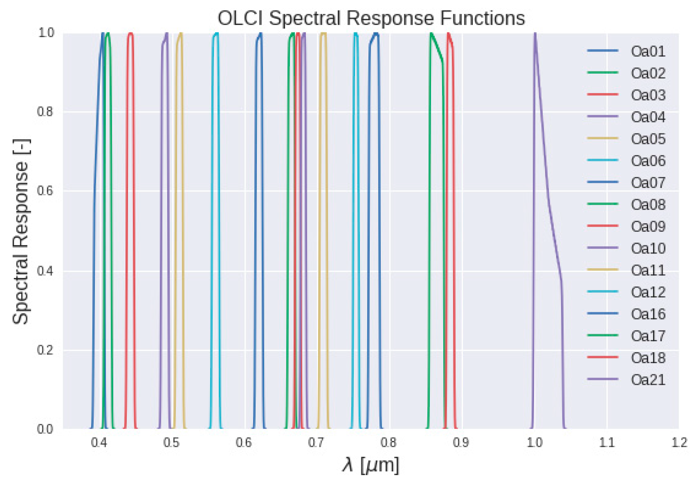
  • OLCI SRF information at 2.5 nm spectral resolution
  • OLCI-observed TOA radiance

6SV V2.1 was installed on a Linux User Virtual Machine in VITO’s Mission Exploitation Platform (MEP) and run for 3 × 3 pixels centered at the AERONET stations’ geolocations. It is emphasized that the distribution of 6SV simulations over the AERONET stations was heavily weighted by the respective stations’ Level 1.5 data availability. As a result, the majority of the simulations were performed over stations located in WEUR [Lille, Palaiseau, Aubière (all France), and Chilbolton (UK)].

3.2.3. RadCalNet Observations

The Radiometric Calibration Network (RadCalNet) is an initiative of the Committee on Earth Observation Satellites (CEOS) Working Group on Calibration and Validation (WGCV) and the Infrared Visible Optical Sensors Subgroup (IVOS). RadCalNet automatically collects in-situ measurements of the bottom of atmosphere (BOA, equivalent to TOC) reflectance at nadir-view and atmospheric parameters, such as surface pressure, TCWV, columnar ozone, AOT, and the Ångström coefficient. The RadCalNet processor ingests in-situ reflectance and atmospheric observations to derive TOA reflectance that is generally used for post-launch radiometric calibration and validation of optical imaging sensor data [15]. In this study, only TOC reflectance data were considered and intercompared with iCOR TOC reflectances. The TOC reflectance from RadCalNet is provided at 10 nm spectral intervals from 0.4–2.5 μm (depending on the site’s instrumentation). It is acquired every 30 min between 09:00 and 15:00 Local Standard Time (LST) and only in cloud-free conditions (

Table 2. RadCalNet site descriptions.

Site Name	Site Owner	Instrumentation Maintenance	Location	Spectral Range (μm)	Surface Reflectance Variability at 500 × 500 m (%)
Railroad Valley(RVUS)	United States Bureau of Land Management (BLM)	Remote Sensing Group- College of Optical Sciences University of Arizona (USA)	Nevada, USA	0.4–2.5	1
Gobabeb (GONA)	Gobabeb Research and Training Centre	National Physical Laboratory (UK)	Naukluft National Park, Namibia	0.4–1.81 1.92–2.3	3

). The network currently includes four sites located in the USA, France, China, and Namibia. A new sandy site in China called Baotou has recently been added.

In this study, the choice of sites suitable for the intercomparison analysis is based on the assessment of the “surface reflectance variability” at 500 × 500 m². Considering that a Sentinel-3 OLCI FR pixel is approximately 300 m, a surface reflectance variability less than 3% is considered acceptable for the analysis, resulting in only the Gobabeb (GONA, Lat: 23.600°S, Lon: 15.119°E) and Railroad Valley (RVUS, Lat: 38.497°N, Lon: 115.690°W) sites considered suitable for this research. GONA and RVUS are desert sites, characterized by sand and gravel with some widely scattered dry grass, and by a high-desert playa surrounded by mountains, respectively. The current uncertainty estimates in the in-situ surface reflectance measurements are 3.5–5.3% for RVUS and 3.5–5.0% for GONA. Figure 2 shows the average and standard deviation in TOC reflectance measured at GONA (black) and RVUS (red) over the considered time over the two sites. The plots demonstrate a high reflectance stability over time, with standard deviations of ~0.02 at GONA and ~0.03 at RVUS.

More information on RadCalNet, its instrumentation, and analysis procedures can be found in [15].

3.2.4. Sentinel-3 SYN L2

Sentinel-3 Synergy L2 (SYN L2) products are provided in Non-Time Critical timeliness (NTC, available 30–48 h after acquisition) and include daytime and land-only datasets. Surface reflectance and aerosol parameters are provided on a 300 m regular ortho-geolocated grid, similar to the OLCI L2 products. Some sub-sampled annotations (solar and viewing azimuth/zenith angles) and meteorological data (mean sea-level pressure, total column ozone, and water vapor, all derived from ECMWF data) are also provided in the OLCI tie points data grids.

TOC reflectances and their associated error estimates are provided for each solar SLSTR and OLCI channel, except for the oxygen absorption bands Oa13, Oa14, and Oa15, the water vapor absorption bands Oa19 and Oa20, and the dedicated SLSTR S4 cloud detection band. Aerosol parameters, such as AOT at 0.550 μm (referenced as T550) and Ångström coefficient around this wavelength (referenced as A550) are included in separate files and are also provided on a 300 m resolution grid. The datasets are associated with contextual parameters, such as geographical position, time stamps, quality flags concerning the SYN L2 processing and OLCI and SLSTR input quality, and classification flags.

3.3. Validation Methods

3.3.1. Sampling Strategy

For the intercomparison of iCOR and SYN L2 TOC retrievals with corresponding 6SV TOC reflectance simulations, for each AERONET station and OLCI band only dates at which iCOR, SYN L2, and the AERONET data (to calculate the 6SV reference TOC reflectance) were available were selected. Subsequently, for the three datasets the arithmetic mean and standard deviation were computed for those pixels in the 3 × 3-pixel area centered at the station’s geolocation for which both SYN L2 and iCOR had valid values.

In the pairwise data extraction for the statistical consistency analysis at frame level, systematic subsampling was performed to reduce the number of data points, extracting every 10th pixel in the X and Y directions. For the statistical analysis over all ROIs and PDUs, an additional random sampling of 2% was applied.

The CLOUD_flags layer as included in the SYN L2 product (CLOUD, CLOUD_AMBIGUOUS, CLOUD_MARGIN, and SNOW_ICE) is used to exclude observations perturbed by clouds or snow/ice. Because currently no list of recommended flags when interpreting SYN L2 data is available, no additional flagging based on SYN L2 flag bands was applied. However, SYN L2 observations with negative AOT at 0.55 μm (~0.002% of the pixels) were discarded.

3.3.2. Vegetation Indices

Per iCOR and SYN L2 frame and for each extraction, the Normalized Difference Vegetation Index (NDVI), Normalized Difference Water Index (NDWI), and Enhanced Vegetation Index (EVI) were computed, based on the Oa03 (Blue), Oa09 (Red), Oa17 (NIR) and Oa21 (SWIR) bands.

$$NDVI=\frac{NIR-Red}{NIR+Red}$$

(2)

$$NDWI=\frac{NIR-SWIR}{NIR+SWIR}$$

(3)

$$EVI=\frac{2.5\ast \left(NIR-Red\right)}{NIR+6\ast Red+7.5\ast Blue+1}$$

(4)

By applying the ratios in these vegetation indices (VIs), any ‘noise’ resulting from the observation geometry (directionality) is expected to be reduced, because these directional effects are similar in the visible and near-infrared bands [21], thereby providing a better indication on the temporal variations.

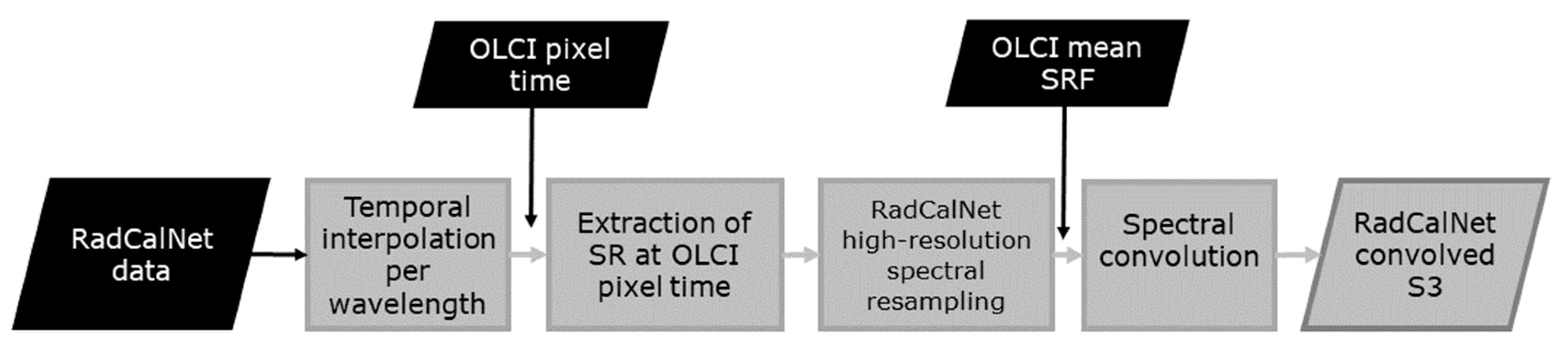
3.3.3. RadCalNet Intercomparison

The methodology adopted for comparing iCOR OLCI TOC reflectances with in-situ RadCalNet observations followed an approach similar to [22]. First, OLCI Level-1 data were selected considering cloud-free conditions over the RadCalNet sites and satellite in -situ data availability. OLCI-L1 FR selected data were then processed using iCOR4S3 deployed on ESA’s G-POD. Afterwards, the iCOR OLCI TOC reflectance and satellite acquisition time from the pixel over the RadCalNet sites were extracted. Finally, the RadCalNet TOC reflectance data were convolved using the OLCI mean SRF and interpolated in time to the satellite overpass time, before comparing the two datasets. A description of the workflow is provided below, while the workflow is depicted in Figure 3.

• RadCalNet TOC reflectances were cubically interpolated from 30 min to 1 sec for every wavelength;
• TOC reflectance values at different wavelengths were extracted at the sensor overpass time;
• TOC reflectances from point 2 were cubically interpolated from 10 nm to 0.1 nm (${\rho }_{\lambda }^H)$;
• TOC reflectances from point 3 were convolved with the OLCI mean SRF ($SR{F}_{\lambda }$), using Equation (5) [22]:

  $${\rho }_{RC}=\frac{{{\displaystyle \sum }}_{{\lambda }_1}^{{\lambda }_2}{\rho }_{\lambda }^H \times SR{F}_{\lambda }}{{{\displaystyle \sum }}_{{\lambda }_1}^{{\lambda }_2}SR{F}_{\lambda } }$$

  (5)

In Equation (5), ${\rho }_{\lambda }^H$ is the interpolated TOC reflectance, $SR{F}_{\lambda }$ is the mean OLCI SRF, and λ₁ and λ₂ define the OLCI band delimitation wavelengths at Full Width at Half Maximum (FWHM). Finally, ${\rho }_{RC}$ is the convolved RadCalNet TOC reflectance converted into the OLCI spectral bands.

3.3.4. Validation Metrics

The validation metrics used in the intercomparison are listed in

Table 3. List of validation metrics, with n the number of valid samples used for the comparison, $\sigma \left(X\right)$ and $\sigma \left(Y\right)$ the standard deviation of $X$ and $Y$, $\sigma \left(X,Y\right)$ the co-variation of $X$ and $Y$, and $\widehat{X}$ and $\widehat{Y}$ estimated using the GM regression model. $P\left(d_i\right)$, $P\left(d_{i+1}\right)$ and $P\left(d_{i+2}\right)$ are three consecutive observations on dates $d_i$, $d_{i+1}$, and $d_{i+2}$.

Validation Metric	Formula
Accuracy (Acc) or mean bias	$Acc=\frac{1}{n}{\displaystyle {\displaystyle \sum }_{i=1}^n}{X}_i-Y_i$
Precision (Prec) or repeatability	$Prec=\sqrt{\frac{1}{n-1}{\displaystyle {\displaystyle \sum }_{i=1}^n}{\left(X_i-Y_i-Acc\right)}^2}$
Uncertainty (Unc) or Root Mean Squared Difference (RMSD)	$Unc=RMSD=\sqrt{\mathrm{MSD}}=\sqrt{\frac{1}{n}{\displaystyle {\displaystyle \sum }_{i=1}^n}{(X_i-Y_i)}^2}$
Root of the unsystematic mean product difference (RMPDu)	$RMP{D}_u=\sqrt{MP{D}_u}=\sqrt{\frac{1}{n}{\displaystyle {\displaystyle \sum }_{i=1}^n}\left(\left|X_i-{\widehat{X}}_i\right|\right)\left(\left|Y_i-{\widehat{Y}}_i\right|\right)}$
Root of the systematic mean product difference (RMPDs)	$RMP{D}_s=\sqrt{MSD-MP{D}_u}$
Coefficient of determination (R2)	$R^2={\left(\frac{\sigma \left(X,Y\right)}{\sigma \left(X\right)·\sigma \left(Y\right)}\right)}^2$
Temporal smoothness (δ)	$\delta \left(d_i\right)=\left|P\left(d_{i+1}\right)-P\left(d_i\right)-\frac{P\left(d_i\right)-P\left(d_{i+2}\right)}{d_i-d_{i+2}}\left(d_i-d_{i+1}\right)\right|$
Time series smoothness index (TSI)	$TSI= \sqrt{\frac{{{\displaystyle \sum }}_{i=1}^{\mathrm{n}-2}\delta {\left(d_i\right)}^2}{n-2}}$
Relative difference [Δ, %]	$\Delta [\%] = \frac{X_i-Y_i}{Y_i}$

. To quantify the deviation between iCOR, SYN L2 TOC reflectances and the 6SV reference simulations, and between iCOR or SYN L2 AOT and the AERONET AOT, the Accuracy, Precision, and Uncertainty (often abbreviated as APU) statistical metrics [23] were calculated. For these cases, X refers to the reference (6SV, RadCalNet or AERONET), and Y to iCOR or SYN L2.

To identify the relationship between iCOR and SYN L2 TOC reflectances and AOT, the geometric mean (GM) regression model is used. Such an orthogonal (model II) regression is appropriate, because—unlike when comparing to an absolute reference—both datasets are subject to noise. By applying an eigen decomposition to the X (SYN L2) and Y (iCOR) covariance metrics, two eigenvectors are obtained that describe the principal axes of the point cloud [24], i.e., the regression line. The GM regression intercept and slope value are added as quantitative information related to the scatterplots. The Root Mean Squared Difference (RMSD) expresses the difference magnitude between two datasets from 0 and is an expression of the overall difference, similar to the Uncertainty.

The GM regression model is also used to differentiate between systematic and random differences, providing additional information on the difference’s nature between two datasets. In order to be comparable to the RMSD’s magnitude, the root of the systematic and unsystematic mean product difference is used (RMPD_s and RMPD_u). The coefficient of determination (R²) indicates the agreement or covariation between two datasets with respect to the linear regression model, summarizing the total explained variance by this model.

The temporal smoothness δ [21,25] of AOT, TOC reflectance, and the VI time series is a measure for its consistency throughout time. Temporal smoothness is evaluated by taking three consecutive observations and by computing the absolute difference value between the center P(d_n+1) and the corresponding linear interpolation between the two extremes P(d_n) and P(d_n+2) The Time Series Smoothness Index (TSI) is an estimate of the time series noise [26], and is defined such that a lower value indicates less temporal noise and thus a smoother time series profile.

4. Results

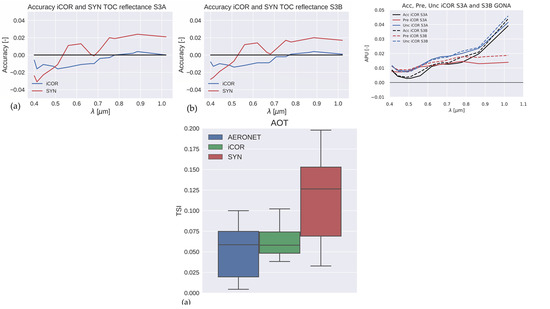
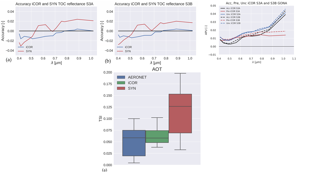
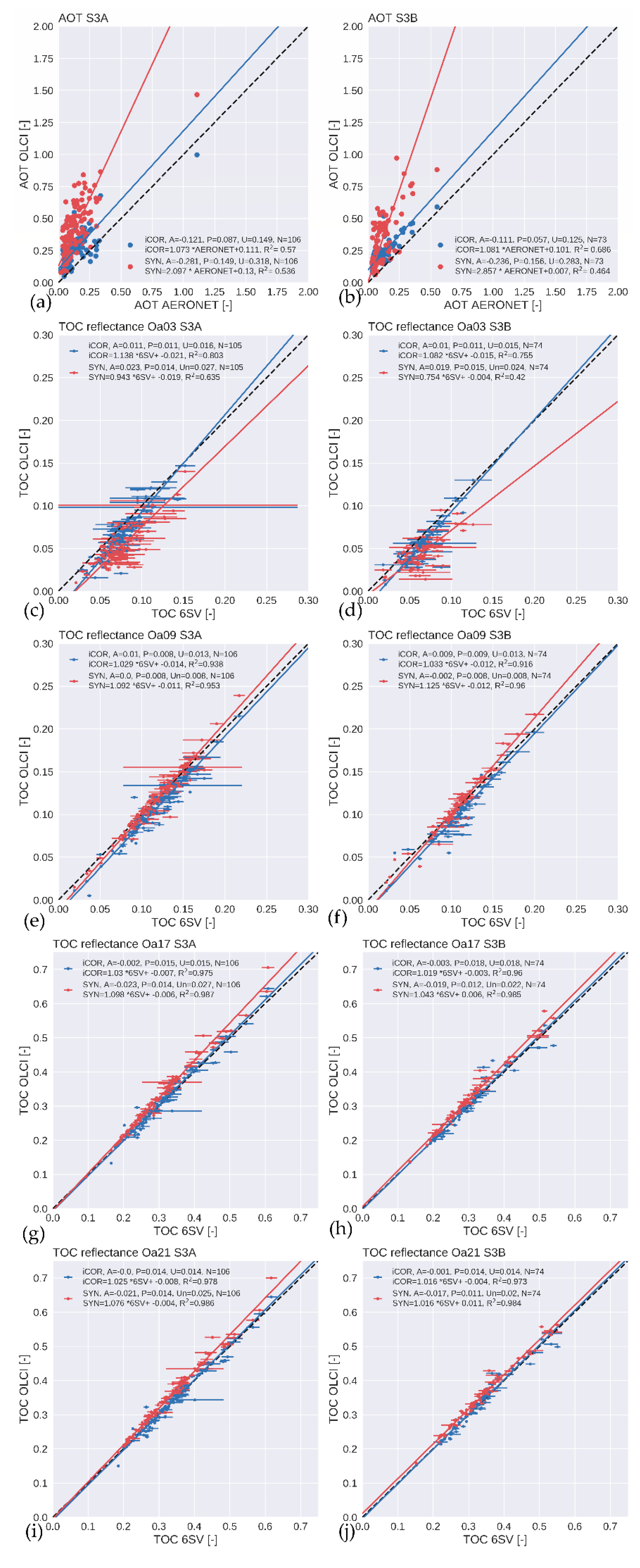
4.1. Intercomparison with 6SV Simulations Using AERONET Input

Figure 4 shows the AOT and TOC reflectance intercomparison between iCOR and SYN (Y axis) with AERONET and 6SV, respectively (X axis), for S3A (left column) and S3B (right column) and for OLCI bands Oa03, Oa09, Oa17, and Oa21.

Table 4. Number of selected data points for the intercomparison of iCOR and SYN with AERONET and 6SV. The number of data points before filtering on AERONET data availability are given between parentheses.

ROI	S3A	S3B	TOTAL
WEUR	90 (194)	57 (164)
NAUS	3 (51)	9 (66)
NBRA	4 (41)	2 (32)
CHIN	9 (25)	6 (12)
TOTAL	106 (311)	74 (374)	180 (685)

presents the number of selected data points included for the intercomparison, separated for S3A and S3B. Note that for CAFR (Bujumbura) no collocations were found for both S3A and S3B, resulting from both quasi-persistent cloud coverage and irregular AERONET observations in general. In the TOC reflectance scatterplots, the error bars in the X direction span the standard deviation of the 6SV-simulated TOC reflectances over the four aerosol models (continental, maritime, urban, and desert).

The scatterplots show that both iCOR and SYN AOT retrievals overestimate relative to AERONET for both S3A and S3B, but that the SYN AOT overestimation is substantially larger. Further, the SYN AOT retrievals for S3B have a larger overestimation than for S3A. Another observation is that for S3B, iCOR AOT > SYN AOT for very low AERONET AOT (<~0.1). The larger overestimation for SYN compared to iCOR also reflects in higher (less favorable) APU values than iCOR. For S3A, the APU values for iCOR (SYN) are 0.12 (0.29), 0.09 (0.16), and 0.15 (0.33), while for S3B these values for iCOR (SYN) are 0.11 (0.24), 0.06 (0.16), and 0.13 (0.28).

For the Blue band (Oa03) TOC reflectances, both SYN and iCOR generally exhibit an underestimation, with the SYN underestimation being larger, especially for S3B. This underestimation gradually reduces with increasing wavelength, due to decreasing aerosol contribution to atmospheric scattering and absorption. Further, the sometimes large error bars for the 6SV TOC reflectance indicate a large spread in the obtained 6SV TOC reference reflectances when different aerosol models are applied. This aerosol model susceptibility indicates that additional research on dynamic aerosol model application for iCOR (which currently uses the MODTRAN rural aerosol model) could be beneficial to further optimize the iCOR TOC reflectance retrieval performance. For Oa09 (Red), the SYN and iCOR TOC reflectances are generally in good agreement with their 6SV counterparts, with a marginal positive bias (Acc = 0–0.002) for SYN, while iCOR shows a slight negative bias (Acc = ~−0.01). For Oa17 and Oa21 (NIR), agreement between SYN, iCOR, and 6SV has increased, which can be expected due to the small aerosol contributions in these bands. iCOR results show virtually no bias relative to 6SV, while for SYN a slight positive bias is seen (Acc = +0.017 and Acc = +0.021 for S3A and S3B, respectively).

The APU and R² spectral signatures are shown in Figure 5. The results are presented separately for S3A and S3B in the left and right columns, respectively. For all statistical metrics, a similar signature can be seen for S3A and S3B. For Accuracy, SYN has lower negative values (larger negative bias) than iCOR up to ~0.5 μm. Further, the SYN negative bias changes into positive from ~0.55 μm onwards, while for iCOR a small negative bias remains until 0.8 μm, becoming slightly positive beyond this wavelength. The Precision evolution for iCOR and SYN is similar, especially for S3A. However, for S3B differences in Precision are larger, with SYN > iCOR up to ~0.65 μm and iCOR > SYN beyond this wavelength, with differences further increasing (i.e., more scattered TOC reflectance retrievals) for λ > 0.75 μm. Uncertainty is larger for SYN compared to iCOR in the BLUE and NIR channels, which indicates a larger spread for SYN. The R² increases towards 1 for both iCOR and SYN with increasing wavelength, with SYN having lower values than iCOR at λ < 0.55 μm, with this difference being more prominent for S3B.

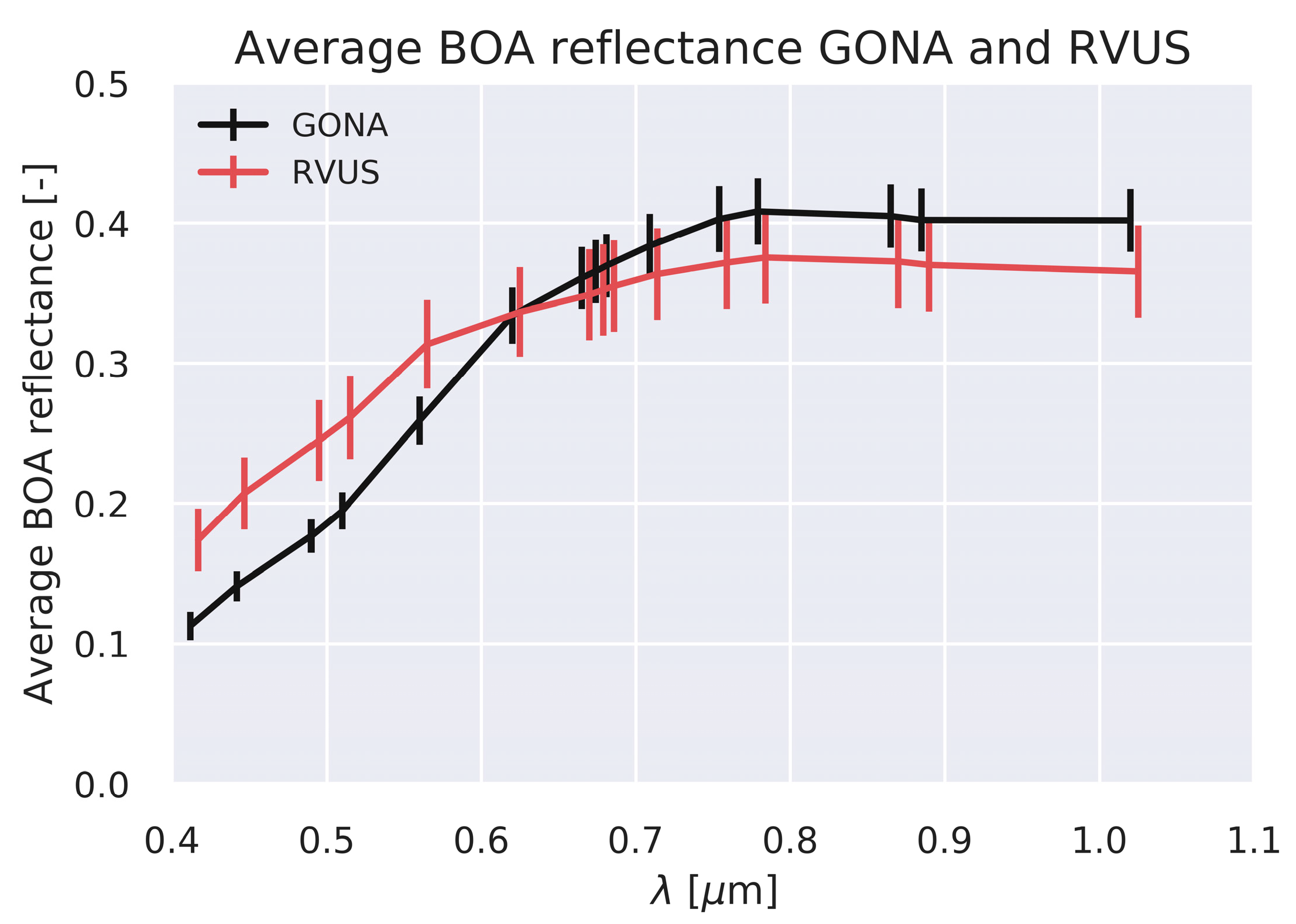
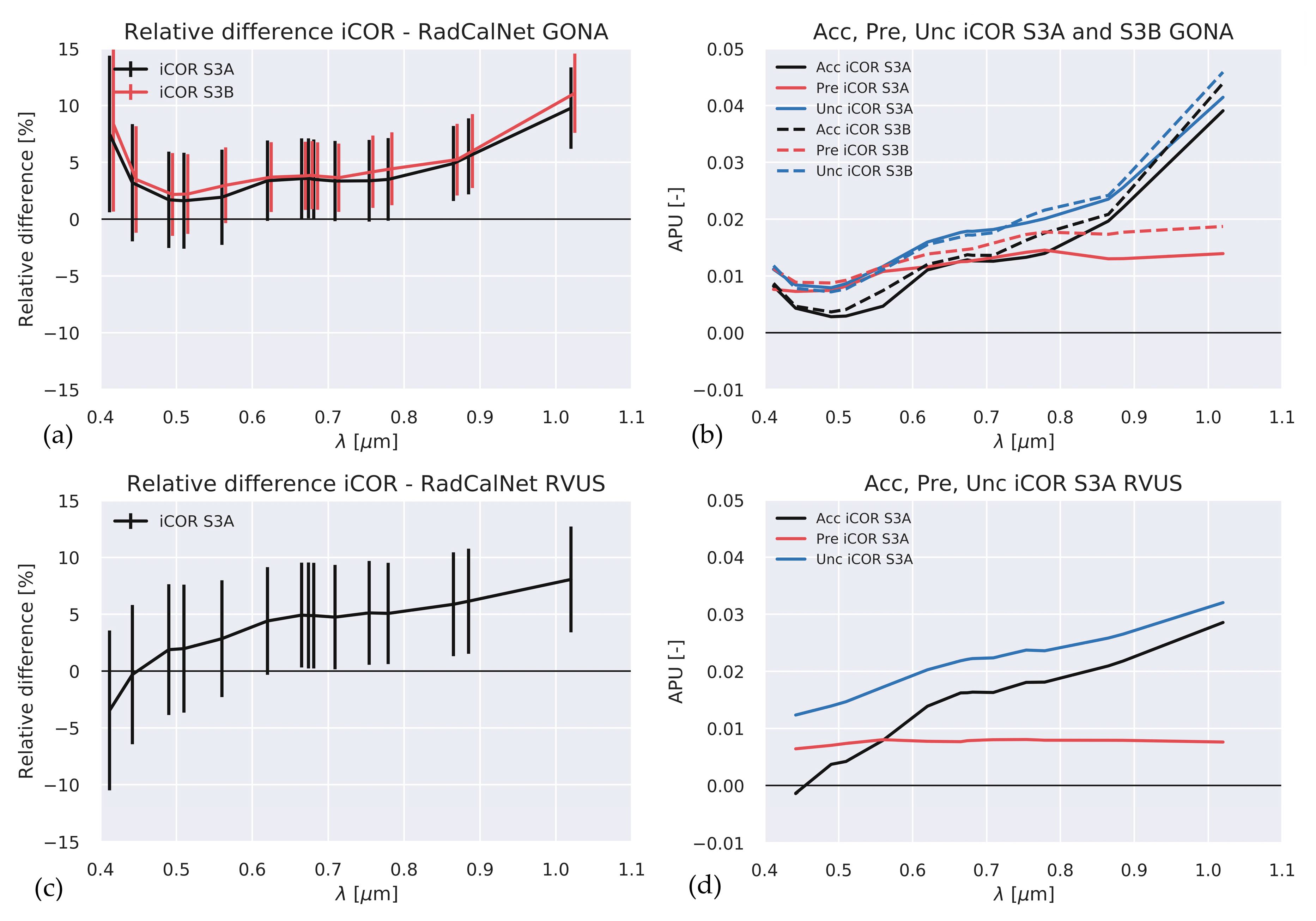
4.2. Intercomparison with RadCalNet Observations

iCOR OLCI TOC reflectances were intercompared with convolved RadCalNet TOC reflectances at the GONA and RVUS sites, following the methodology described in Section 3.3.4. Initially, to reduce any Bi-directional Reflectance Distribution Function (BRDF) impact, only satellite images over the RadCalNet sites with VZA < 10° were considered. However, this constraint provided only a few matchups. Thanks to an ad-hoc processing by the Centre National d’Études Spatiales (CNES) that provided BRDF-corrected data in OLCI acquisition geometry [27], all possible VZAs could be considered, which allows for inclusion of more matchups in the analysis. The former approach was applied to the RVUS site, the latter to the GONA site.

Table 5. Number of Sentinel-3 products selected considering the in-situ data availability and cloud-free conditions. (*) Sentinel-3 OLCI-L1 B reprocessed data by Centre National d’Études Spatiales (CNES).

Sensor	RVUS	GONA	RVUS Time Interval	GONA Time Interval
OLCI S3A	17	63	04/09/2016–09/07/2020	21/07/2017–01/10/2019
OLCI S3B	-	38 *	-	15/12/2018–08/10/2019

shows the datasets used in the analysis for the two sites.

Given the OLCI FR data 300 m resolution and the surface reflectance variability at the RadCalNet sites, the iCOR TOC (surface) reflectance values were extracted for 1 pixel at GONA and for an average of 3 × 3 pixels centered at RVUS.

Figure 6 shows the average relative difference and standard deviation at (a) GONA and (b) RVUS, together with (c,d) the corresponding APU values for GONA and RVUS, respectively. Band Oa01 (0.4 μm) was excluded from the analysis, because the RadCalNet acquisitions start from 0.400 μm and the OLCI SRF for Oa01 starts from 0.388 μm.

In general, at GONA the average relative differences are within ±6% for all bands, except for Band Oa02 (0.412 μm) and Oa21 (1.02 μm). The larger relative difference of these two bands relate to OLCI S3A having an “excess of brightness”, mainly in the Blue bands and the Oa21 (NIR) band (see https://sentinel.esa.int/web/sentinel/technical-guides/sentinel-3-olci/mission-performance, accessed 18 November 2020). It is emphasized that, because in the comparison with the 6SV TOC reflectance simulations (see Section 4.1) both iCOR and 6SV start from the OLCI Level 1B data, the excess of brightness is present in both datasets and is thus cancellated in the intercomparison results. iCOR on OLCI S3A and OLCI S3B show similar values, also when the dataset contains a different number of products. Figure 6b shows that the Accuracy and Uncertainty for bands Oa17, Oa18, and Oa21 are higher (implying less agreement) than for the other bands, reaching Oa21 Accuracy (Uncertainty) peak values of 0.039 (0.041) and 0.044 (0.046) for iCOR on S3A and S3B, respectively.

At the RVUS site (Figure 6c,d), the average relative differences are within ±6% for all bands, similar to GONA, except for Oa21 (+8%). Band Oa02 shows a negative difference (−3.5%) in comparison with the GONA TOC reflectances. This means that for Oa02 iCOR surface reflectance overestimates at GONA and underestimates at RVUS. Concerning the APU, Accuracy and Uncertainty show a gradual increase with wavelength. Accuracy (Uncertainty) maximum values are 0.029 (0.032) for band Oa21. The Precision shows values <0.01 for all bands.

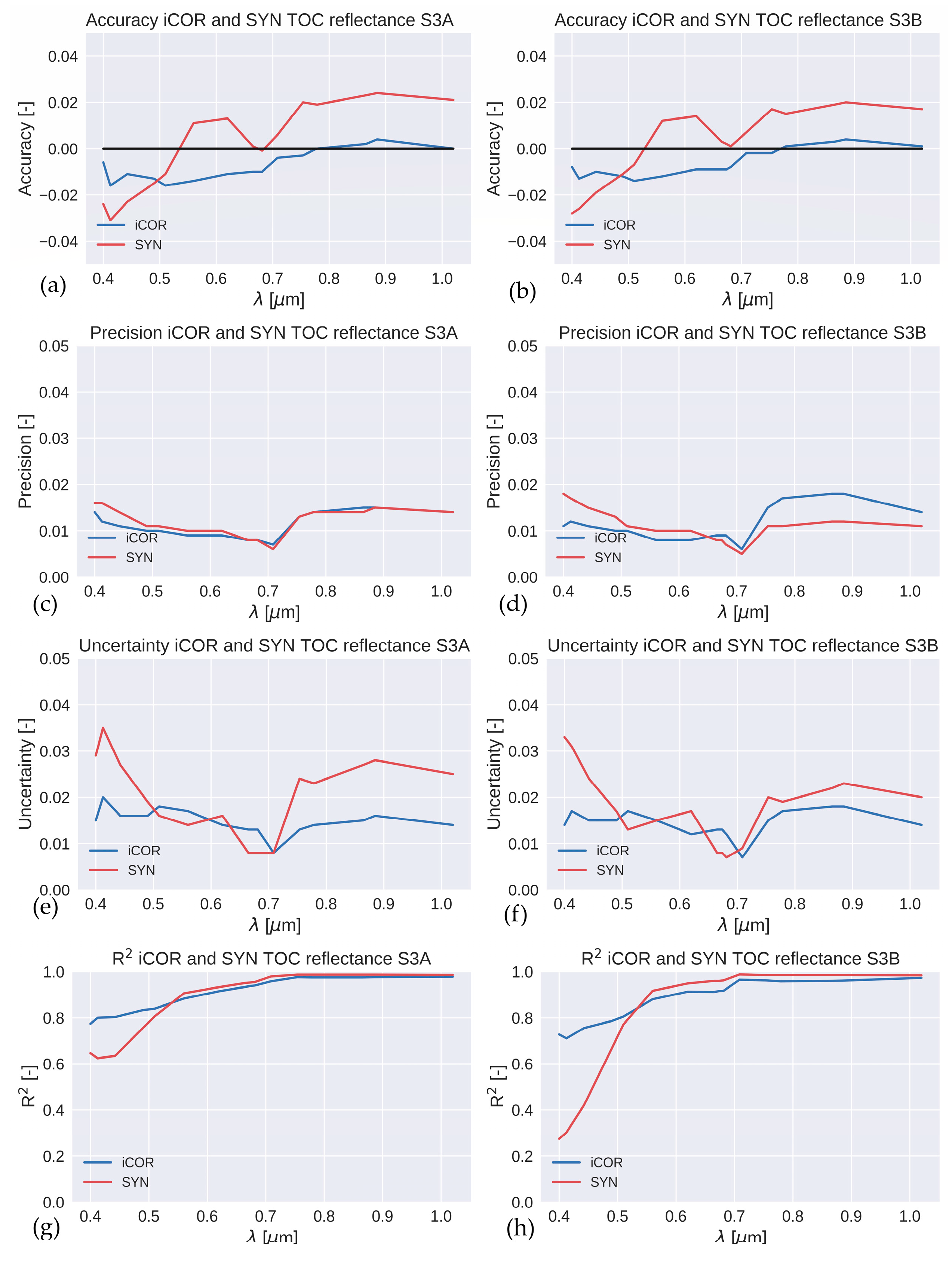
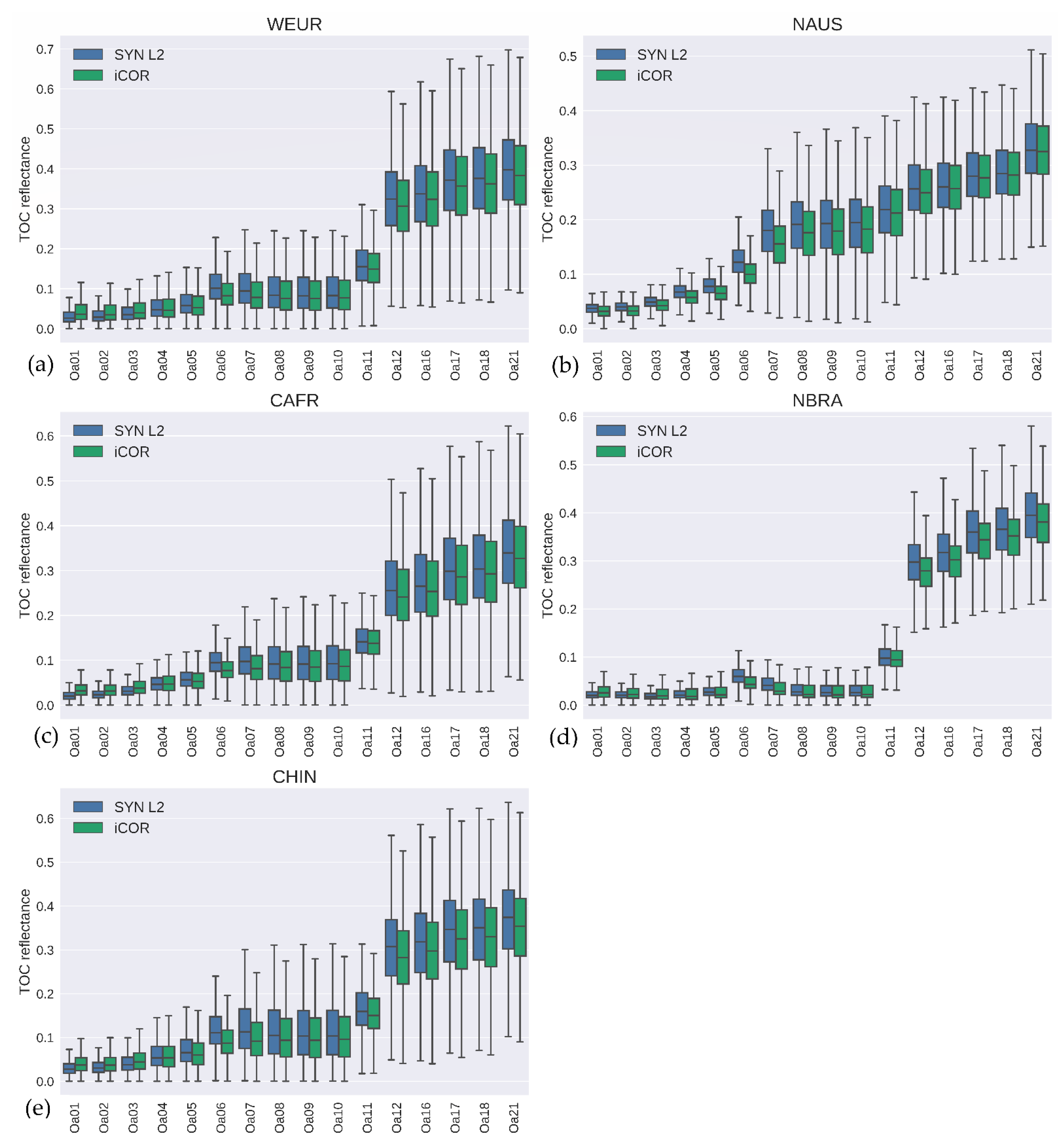
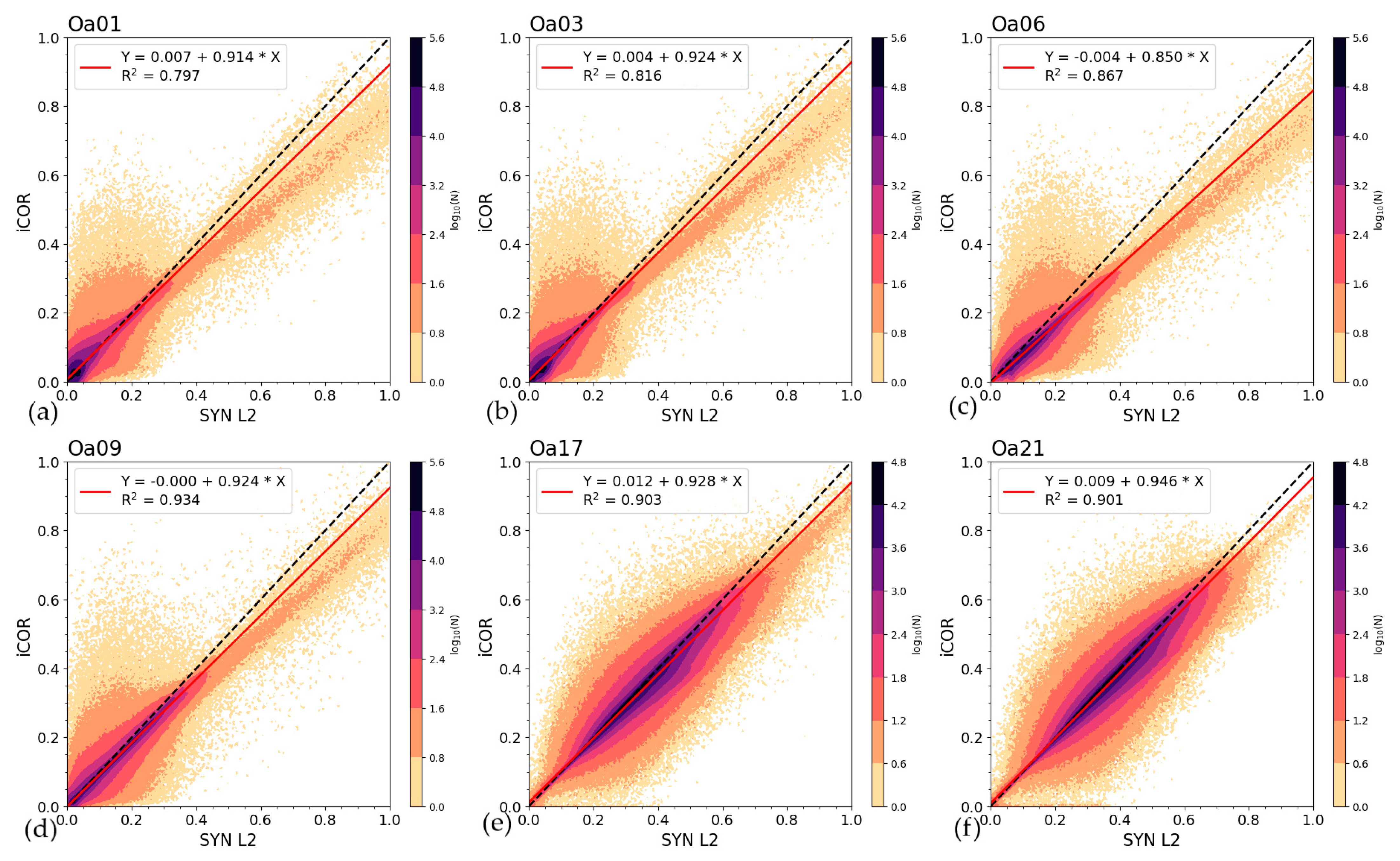
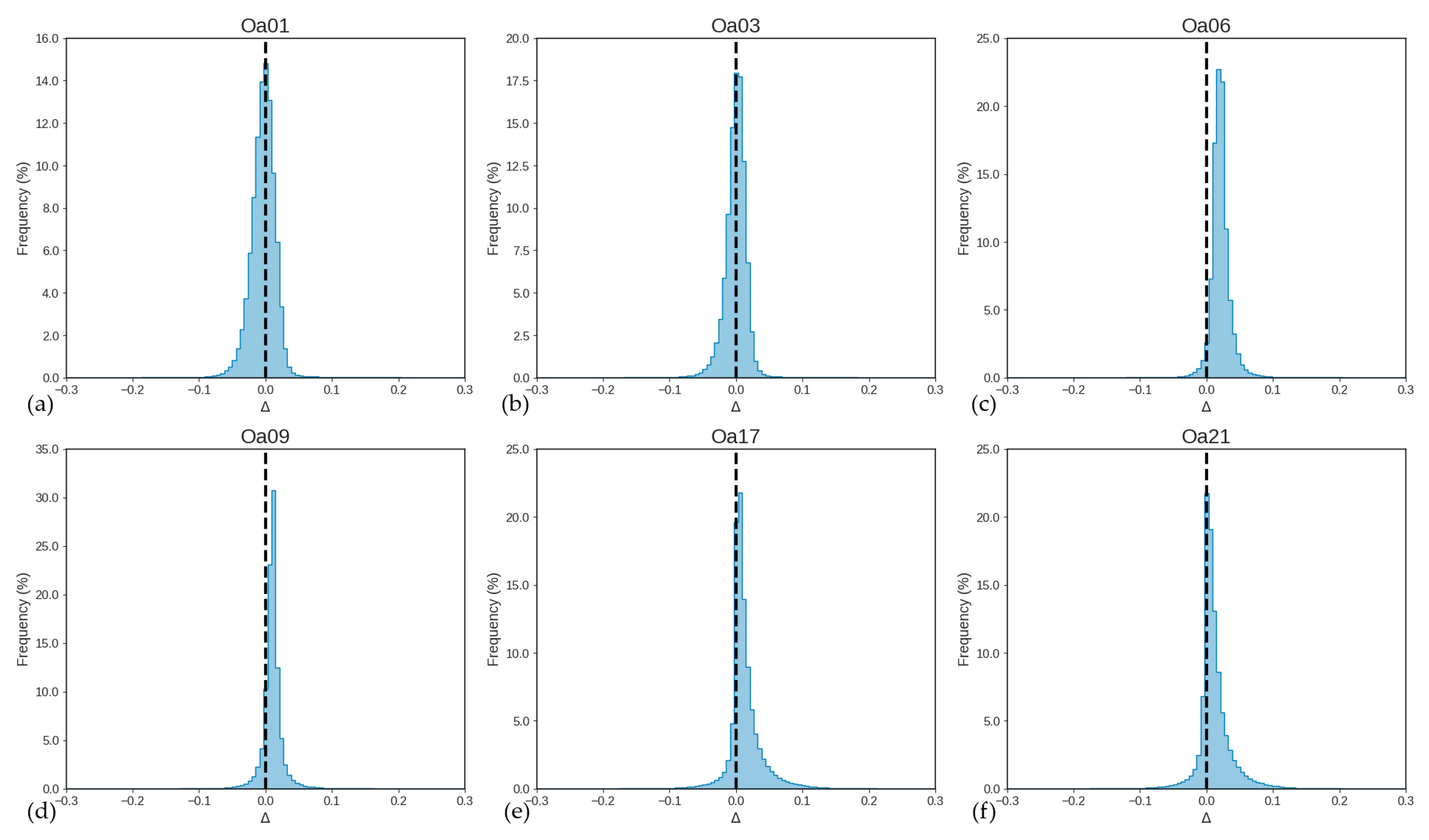
4.3. Intercomparison with Sentinel-3 SYN L2

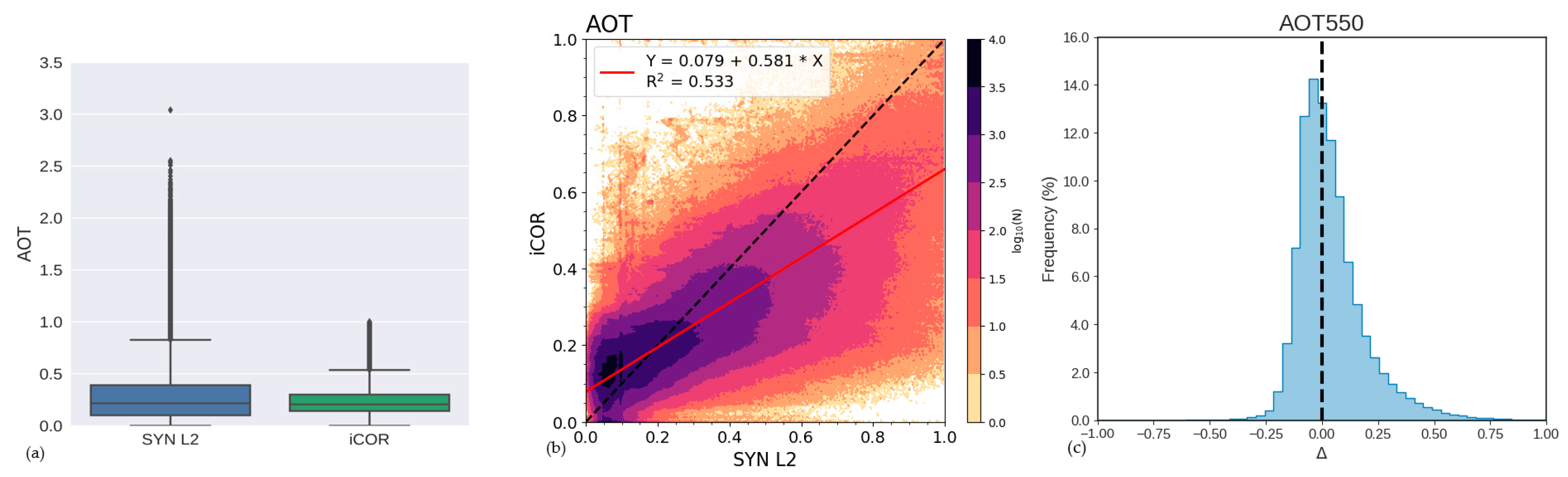
4.3.1. Statistical Consistency iCOR Versus SYN L2

Figure 7 shows (a) the iCOR versus SYN L2 AOT boxplot, (b) GM regression density plot, and (c) the bias frequency histogram. The boxplot shows a slightly lower median AOT for iCOR and a larger AOT interquartile range for SYN L2. In addition, the SYN L2 AOT maximum value is much higher, with outliers up to AOT = 3.2. Similar results were observed over all ROIs, except for NAUS, where AOT is generally low, interquartile ranges very small, and iCOR having slightly higher AOT than SYN L2. The GM regression density plot indicates relatively good AOT consistency for values around 0.2. iCOR exhibits higher values than SYN L2 for AOT <~0.2, while the opposite occurs at larger AOT. As for the boxplots, similar results are observed over all ROIs, except for NAUS. The AOT bias frequency histogram shows that the histogram is skewed towards positive values, indicating for a relatively large proportion of pixels with SYN L2 AOT > iCOR AOT.

Table 6. Validation metrics for the iCOR versus SYN L2 AOT intercomparison.

ROI	N	Intercept	Slope	R2	RMSD	RMPDu	RMPDs
All	8.87 × 106	0.079	0.581	0.533	0.144	0.125	0.072
WEUR	1.48 × 107	0.113	0.401	0.323	0.176	0.142	0.104
NAUS	1.48 × 107	0.104	0.403	0.141	0.098	0.097	0.013
CAFR	3.20 × 106	0.125	0.537	0.335	0.146	0.132	0.062
NBRA	8.04 × 106	0.028	0.799	0.706	0.130	0.119	0.052
CHIN	3.42 ×106	0.131	0.515	0.382	0.190	0.158	0.105

summarizes the validation metrics overall and per ROI. For all ROIs, intercepts are above 0 and slopes are below 1. Bias is lowest for NAUS and highest for CHIN. The systematic differences (RMPDs) are large compared to the RMSD, i.e., the difference between the regression line and the 1:1 line is large.

TOC reflectance boxplots per band (Figure 8) show that for all ROIs the iCOR interquartile range is larger than SYN L2 in bands Oa01–Oa05. Except for NAUS, the iCOR TOC reflectances are slightly higher in bands Oa01–Oa03. NAUS is a particular case because the AOT in general is very low and the iCOR AOT values are higher than SYN L2 AOT (see Figure 7). For bands Oa06–Oa21, iCOR has a lower value range, and the TOC reflectances are lower. These findings are in line with the intercomparison results over the AERONET sites (Figure 4).

The GM regression density plots over all ROIs (Figure 9) show intercepts close to 0, indicating that high consistency is achieved for low TOC reflectance values. Slopes are generally below 1, i.e., with increasing reflectance values SYN L2 becomes increasingly higher than iCOR. These differences at higher reflectances are larger at the shorter wavelengths.

The bias frequency histograms (Figure 10) show that the bias between SYN L2 and iCOR reflectances is centered around 0, except for Oa06 and Oa09, indicating a systematic bias for these intermediate wavelengths. This is confirmed in Figure 11, which shows the overall systematic (RMPDs) and unsystematic difference (RMPDu) as functions of wavelength. The systematic bias (the difference between the regression line and the 1:1 line) is relatively low for the Blue bands and beyond ~0.75 μm and shows a peak at intermediate wavelengths, whereas the unsystematic bias (i.e., scatter) is virtually unrelated to wavelength. For both RMPDs and RMPDu, examination of the separate ROIs (plots are not shown) indicate that the spectral evolutions are similar, except for NAUS, where the systematic bias remains low at longer wavelengths.

The NDVI, NDWI, and EVI bias frequency histograms SYN L2—iCOR (Figure 12) indicate that primarily iCOR NDVI is higher than SYN L2 NDVI. This bias is also visible, although less obvious, for EVI. For NDWI, a slight positive bias (i.e., iCOR NDWI < SYN L2 NDWI) is observed. The mean (standard deviation) differences are −0.019 (0.054), 0.003 (0.008), and −0.001 (0.052) for NDVI, NDWI, and EVI, respectively.

The observed bias results from the band combinations. In both NDVI and EVI, band Oa09 is used, for which the systematic bias iCOR–SYN L2 is smaller compared to the other bands. For the NDWI, only bands Oa17 and Oa21 are used, which both show a similar bias between iCOR and SYN L2. In this case, the band combination thus neutralizes the bias between the TOC reflectances.

A similar conclusion can be drawn from the Geometric Mean Regression (GMR) density plots (Figure 13). Over all ROIs, all VIs show a very high coefficient of determination (R² = 0.92–0.96). The systematic bias between iCOR and SYN L2 NDVI is relatively large (0.01–0.03), resulting from an intercept well above 0 (except for NAUS) and slopes close to 1. The systematic bias is lower for EVI (0.00 to 0.02) and very low for NDWI (below 0.005). The unsystematic bias (i.e., scatter around the regression line) is also larger for NDVI (0.02–0.07) and EVI (0.01–0.07), compared to NDWI (within 0.01).

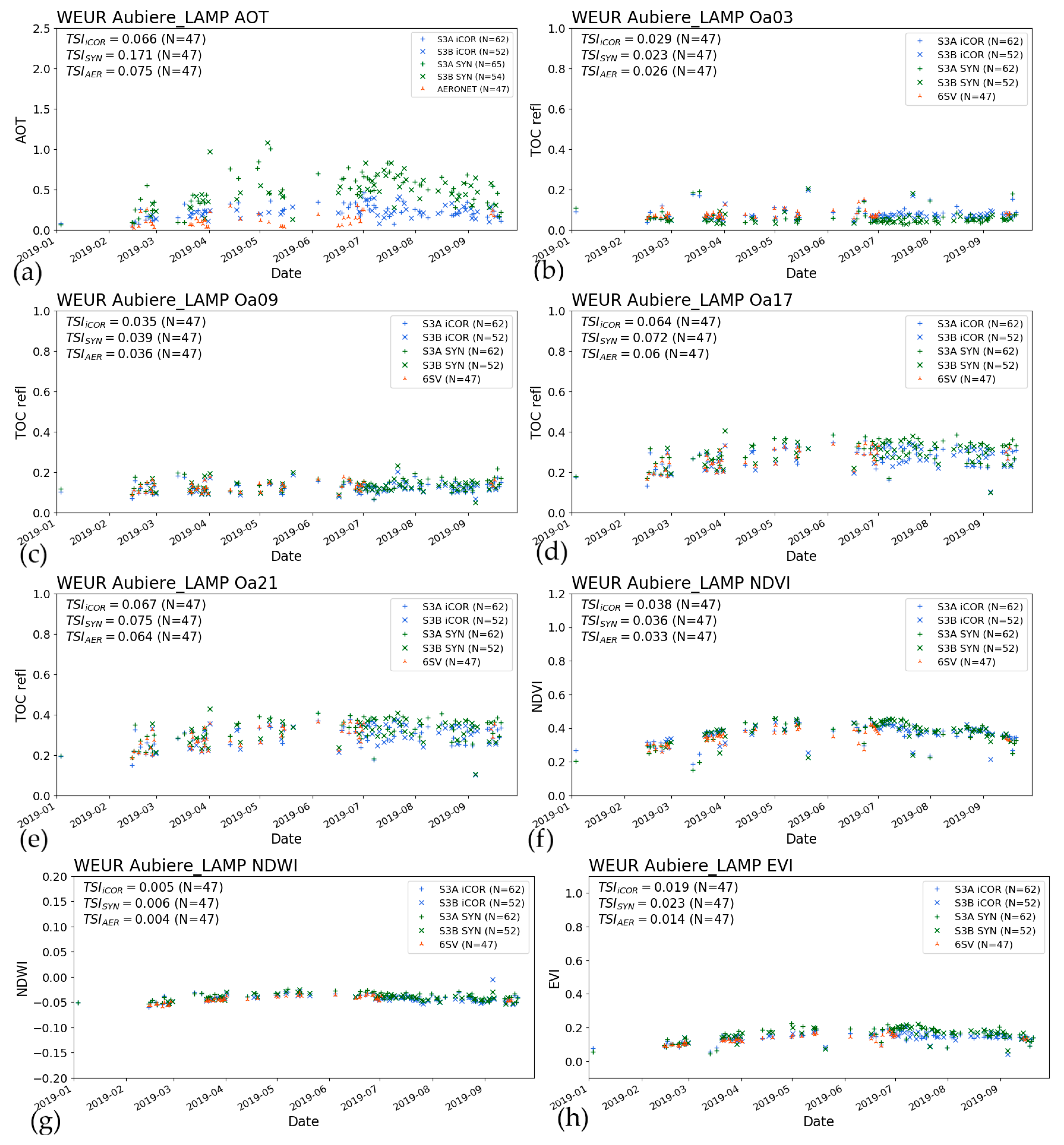
4.3.2. Temporal Consistency iCOR vs. SYN L2

Based on the temporal evolution plots, the TSI was computed over the common valid observations for the 11 AERONET sites. Results are presented in Figure 14 and show that iCOR values are considerably lower than those of SYN L2, indicating a higher AOT temporal smoothness. However, this higher iCOR AOT temporal smoothness does not propagate into a significantly higher temporal smoothness in the TOC reflectance and VI.

An AOT, TOC reflectance, and VIs timeseries example is given in Figure 15 for Aubière LAMP (France, WEUR). For each AERONET station, the TSI was computed over the common valid observations. Figure 15 shows the earlier discussed persistent overestimation of SYN L2 AOT compared to AERONET. In addition, iCOR tends to overestimate AOT, but the difference compared to AERONET AOT is smaller than for SYN L2. This confirms the results presented in Figure 4. For the TOC reflectances, similar temporal patterns for iCOR and SYN L2 are seen. Some outliers are visible, which are possibly related to undetected thin clouds or cloud shadows. In addition, the temporal plots for the VIs show a high degree of similarity. Timeseries over AERONET stations in other ROIs (not shown) reveal a consistent behavior.

5. Discussion

The various intercomparisons generally show a high agreement between iCOR AOT, TOC reflectance, and VIs with the corresponding reference datasets. For AOT, iCOR has a higher agreement with AERONET observations than SYN L2. However, although iCOR has a slightly better agreement with 6SV than SYN L2 for the TOC reflectances, the differences are considerably smaller than for AOT. Despite AOT being important in the atmospheric correction, its impact appears rather limited on the differences between iCOR and SYN L2. iCOR and SYN L2 apply different aerosol models, rural and continental, respectively. As was shown in the 6SV intercomparison results in Figure 4, applying a different aerosol model can substantially affect the obtained TOC reflectance. The rural aerosol model used by iCOR comprises 70% water-soluble and 30% dust-like particles [28], whereas the SYN L2 continental aerosol model from 6S is composed of 29% water-soluble, 70% dust-like, and 1% soot particles [20]. The resulting single scattering albedos are 0.94 and 0.89 for iCOR and SYN L2, respectively, which implies that more of the incoming and outgoing reflected solar irradiance is absorbed for SYN L2, especially in case of multiple interactions within the land surface-atmosphere system. However, it is not straightforward to assess the final effect of this difference, as it depends on, among others, the underlying surface, the AOT (higher probability of multiple scattering events), and atmospheric absorption becoming dominant over scattering with increasing wavelength (see e.g., [29]). The RadCalNet intercomparison shows that over bare desert surfaces iCOR provides consistent results for all bands, except for larger differences in the Blue bands and Oa21 (NIR). However, these larger differences for the mentioned bands can be attributed to the reported “excess of brightness” for OLCI on S3A. As this excess of brightness was observed on various intercomparisons of OLCI-A and OLCI-B TOA observations, any aerosol influence in the Blue would impact both sensors. More information on OLCI-A and -B performance is available in [30]. In the iCOR versus SYN L2 intercomparison, primarily for NDVI a systematic bias was shown, related to the relatively high systematic bias for band Oa17 and low bias for Oa09. In the case of NDWI, the combination using bands Oa17 and Oa21, which have a similar bias, results in a neutralization, thereby resulting in good consistency.

Because iCOR and SYN L2 are currently the only known atmospheric correction algorithms that are applied to Sentinel-3/OLCI observations, any conclusions that arise from this study are preliminary. Nevertheless, as iCOR has participated in ACIX-I [12] and its successor ACIX-II, some additional performance indication for usage on Sentinel-2/MSI is available. In ACIX-I, an AOT overestimation for AERONET AOT <~0.5 was found, which decreased for larger AOT values, resulting in an overall mean AOT difference of 0.15 ± 0.15. For surface reflectance, its retrievals exhibited a small bias compared to AERONET-based 6S TOC reflectance < ~0.2, which increased for brighter surfaces, and resulted in an overall Accuracy (bias) of 0.000 (band 2, 0.492 μm)–0.032 (band 8, 0.833 μm).

6. Conclusions

This paper presented the validation of the iCOR atmospheric correction algorithm applied to Sentinel-3A and -B Ocean and Land Colour Instrument (OLCI) observations over land. iCOR-retrieved Aerosol Optical Thickness (AOT), Top-Of-Canopy (TOC) reflectance, and resulting Vegetation Indices (VIs) were compared with Aerosol Robotic Network (AERONET) AOT, AERONET-based Second Simulation of a Satellite Signal in the Solar Spectrum Vector (6SV)-simulated TOC reflectance, RadCalNet TOC reflectance observations, and corresponding SYN Level 2 (L2) retrievals. The comparisons were performed over 11 AERONET stations and 389 OLCI frames over 5 ROIs: Western Europe (WEUR), Northern Brazil (NBRA), Central Africa (CAFR), Eastern China (CHIN), and Northern Australia (NAUS). The comparisons focused on the statistical and temporal consistency of the retrieved reflectances and VIs. Further, the OLCI iCOR TOC reflectances were compared with collocated and convolved RadCalNet TOC reflectances at the Gobabeb (GONA, Namibia) and Railroad Valley (RVUS, USA) sites.

The intercomparison with observed AOT and 6SV-simulated reference TOC reflectances over AERONET stations reveals that for AOT both iCOR and SYN L2 overestimate relative to AERONET, with the SYN L2 overestimation being larger than for iCOR. For the TOC reflectances in band Oa03 (Blue), both SYN and iCOR generally underestimate, which gradually reduces with increasing wavelength due to the decreasing aerosol contribution on atmospheric scattering and absorption. For Oa09, SYN, iCOR, and 6SV TOC reflectances are generally in good agreement, with only marginal positive and negative bias for SYN and iCOR, respectively. For the NIR bands (Oa17 and Oa21), the iCOR retrievals show virtually no bias relative to 6SV, while SYN shows a slight positive bias.

The intercomparison of iCOR TOC reflectances with RadCalNet convolved TOC reflectance observations showed that there is good consistency for all bands for both S3A and S3B, except for the Oa02 (Blue) and Oa21 (NIR) bands. For the NIR bands, there is an overestimation of iCOR compared to RadCalNet. In Oa02, an over- and an underestimation are seen at GONA and RVUS, respectively.

The statistical consistency analysis between iCOR and SYN L2 confirms the higher AOT for SYN L2 and a larger AOT dynamic range, except for NAUS, where AOT is generally very low. In general, a high consistency between iCOR and SYN L2 is observed at low TOC reflectance values. At higher reflectance values, SYN L2 reflectances are larger than iCOR. Systematic bias is relatively low for the Blue bands and around 0.7 μm. Except for NAUS, the iCOR TOC reflectances are slightly higher in bands Oa01–Oa03. For bands Oa06–Oa21, iCOR has a lower dynamic range and TOC reflectances are lower than SYN L2. Temporal AOT evolution plots from iCOR4S3, SYN L2, and AERONET show a consistent overestimation of SYN L2 AOT, and—to a lesser extent—iCOR relative to AERONET. For the TOC reflectances and VIs, temporal patterns for iCOR and SYN L2 are similar. The iCOR AOT TSI is considerably lower (indicative of less noise) than SYN L2 AOT and is comparable to that of AERONET, but the smoother temporal iCOR AOT pattern does not result in a significantly smoother iCOR TOC reflectance and VIs time series than those of SYN L2.

In conclusion, after the successful validation of iCOR over inland waters, this validation study shows that iCOR applied to Sentinel-3/OLCI also performs well over land surfaces. Overall, a good consistency with the SYN L2 TOC reflectance products is observed. In addition, in comparison to SYN L2, iCOR AOT and TOC reflectance values are shown to be in better agreement with the AERONET AOT and simulated 6SV TOC reflectance reference, respectively. Future iCOR developments will involve: (i) the possibility to include additional aerosol models, and (ii) include Copernicus Atmospheric Monitoring Service (CAMS) AOT data for cases in which the AOT retrieval does not converge to a solution, using a similar approach as for iCOR on Sentinel-2/MSI.

iCOR’s previous operational applications, continuous development, and agility to different processing infrastructures ensure a stable, efficient, and high-quality processing performance, thereby making iCOR suitable for various additional operational implementations.

References

1. Donlon, C.; Berruti, B.; Buongiorno, A.; Ferreira, M.H.; Féménias, P.; Frerick, J.; Goryl, P.; Klein, U.; Laur, H.; Mavrocordatos, C.; et al. The global monitoring for environment and security (GMES) sentinel-3 mission. Remote Sens. Environ. 2012, 120, 37–57. [Google Scholar] [CrossRef]
2. Attema, E.P.W. The active microwave instrument on-board the ERS-1 satellite. Proc. IEEE 1991, 79, 791–799. [Google Scholar] [CrossRef]
3. Louet, J.; Bruzzi, S. ENVISAT mission and system. In Proceedings of the IEEE 1999 International Geoscience and Remote Sensing Symposium, Hamburg, Germany, 28 June–2 July 1999; p. 16. [Google Scholar]
4. Passot, X. VEGETATION image processing methods in the CTIV. Proc. Veg. 2001, 2, 3–6. [Google Scholar]
5. Kravitz, J.; Matthews, M.; Bernard, S.; Griffith, D. Application of Sentinel 3 OLCI for chl-a retrieval over small inland water targets: Successes and challenges. Remote Sens. Environ. 2020, 237, 111562. [Google Scholar] [CrossRef]
6. Pahlevan, N.; Smith, B.; Schalles, J.; Binding, C.; Cao, Z.; Ma, R.; Alikas, K.; Kangro, K.; Gurlin, D.; Hà, N.; et al. Seamless retrievals of chlorophyll-a from Sentinel-2 (MSI) and Sentinel-3 (OLCI) in inland and coastal waters: A machine-learning approach. Remote Sens. Environ. 2020, 240, 111604. [Google Scholar] [CrossRef]
7. Gower, J.; King, S. The distribution of pelagic Sargassum observed with OLCI. Int. J. Remote Sens. 2020, 41, 5669–5679. [Google Scholar] [CrossRef]
8. Wang, X.; Ling, F.; Yao, H.; Liu, Y.; Xu, S. Unsupervised Sub-pixel water body mapping with sentinel-3 OLCI image. Remote Sens. 2019, 11, 327. [Google Scholar] [CrossRef] [Green Version]
9. Zhang, L.; Wylie, B.; Loveland, T.; Fosnight, E.; Tieszen, L.L.; Ji, L.; Gilmanov, T. Evaluation and comparison of gross primary production estimates for the Northern Great Plains grasslands. Remote Sens. Environ. 2007, 106, 173–189. [Google Scholar] [CrossRef] [Green Version]
10. Brown, L.A.; Dash, J.; Lidon, A.L.; Lopez-Baeza, E.; Dransfeld, S. Synergetic Exploitation of the Sentinel-2 missions for validating the Sentinel-3 ocean and land color instrument terrestrial chlorophyll index over a vineyard dominated Mediterranean environment. IEEE J. Sel. Top. Appl. Earth Obs. Remote Sens. 2019, 12, 2244–2251. [Google Scholar] [CrossRef]
11. De Keukelaere, L.; Sterckx, S.; Adriaensen, S.; Knaeps, E.; Reusen, I.; Giardino, C.; Bresciani, M.; Hunter, P.; Neil, C.; Van Der Zande, D.; et al. Atmospheric correction of Landsat-8/OLI and Sentinel-2/MSI data using iCOR algorithm: Validation for coastal and inland waters. Eur. J. Remote Sens. 2018, 51, 525–542. [Google Scholar] [CrossRef] [Green Version]
12. Doxani, G.; Vermote, E.; Roger, J.C.; Gascon, F.; Adriaensen, S.; Frantz, D.; Hagolle, O.; Hollstein, A.; Kirches, G.; Li, F.; et al. Atmospheric correction inter-comparison exercise. Remote Sens. 2018, 10, 352. [Google Scholar] [CrossRef] [PubMed] [Green Version]
13. Renosh, P.R.; Doxaran, D.; de Keukelaere, L.; Gossn, J.I. Evaluation of atmospheric correction algorithms for sentinel-2-MSI and sentinel-3-OLCI in highly turbid estuarine waters. Remote Sens. 2020, 12, 1285. [Google Scholar] [CrossRef] [Green Version]
14. Holben, B.N.; Eck, T.F.; Slutsker, I.; Tanré, D.; Buis, J.P.; Setzer, A.; Vermote, E.; Reagan, J.A.; Kaufman, Y.J.; Nakajima, T.; et al. AERONET—A federated instrument network and data archive for aerosol characterization. Remote Sens. Environ. 1998, 66, 1–16. [Google Scholar] [CrossRef]
15. Bouvet, M.; Thome, K.; Berthelot, B.; Bialek, A.; Czapla-Myers, J.; Fox, N.P.; Goryl, P.; Henry, P.; Ma, L.; Marcq, S.; et al. RadCalNet: A radiometric calibration network for earth observing imagers operating in the visible to shortwave infrared spectral range. Remote Sens. 2019, 11, 2401. [Google Scholar] [CrossRef] [Green Version]
16. Berk, A.; Anderson, G.P.; Acharya, P.K.; Bernstein, L.S.; Muratov, L.; Lee, J.; Fox, M.; Adler-Golden, S.M.; Chetwynd, J.H., Jr.; Hoke, M.L.; et al. MODTRAN5: 2006 Update; Shen, S.S., Lewis, P.E., Eds.; International Society for Optics and Photonics: Bellingham, WA, USA, 2006; p. 62331F. [Google Scholar]
17. North, P.R.J.; Brockmann, C.; Fischer, J.; Gomez-Chova, L.; Grey, W.; Heckel, A.; Moreno, J.; Preusker, R.; Regner, P. MERIS/AATSR synergy algorithms for cloud screening, aerosol retrieval and atmospheric correction. In Proceedings of the 2nd MERIS/AATSR User Workshop, ESRIN, Frascati, Italy, 22–26 September 2008; ESA Publications Division, European Space Agency: Noordwijk, The Netherlands, 2008; pp. 22–26. [Google Scholar]
18. Sterckx, S. iCOR-OLCI Plugin for SNAP Toolbox—Software User Manual, 2019. Available online: https://cdn2.hubspot.net/hubfs/2834550/marketing/MAILS/iCOR/iCORpluginUserManual_OLCI_v1.0.pdf (accessed on 27 October 2020).
19. Vermote, E.F.; Tanré, D.; Deuzé, J.L.; Herman, M.; Morcrette, J.J. Second simulation of the satellite signal in the solar spectrum, 6s: An overview. IEEE Trans. Geosci. Remote Sens. 1997, 35, 675–686. [Google Scholar] [CrossRef] [Green Version]
20. Vermote, E.; Tanre, D.; Deuze, J.L.; Herman, M.; Morcrette, J.J. 6S User Guide Version 3, Appendix III, 55 pp, 2006. Available online: https://ltdri.org/files/6S/6S_Manual_Part_2.pdf (accessed on 28 November 2019).
21. Vermote, E.; Justice, C.O.; Bréon, F.M. Towards a generalized approach for correction of the BRDF effect in MODIS directional reflectances. IEEE Trans. Geosci. Remote Sens. 2009, 47, 898–908. [Google Scholar] [CrossRef]
22. Jing, X.; Leigh, L.; Pinto, C.T.; Helder, D. Evaluation of RadCalNet output data using Landsat 7, Landsat 8, Sentinel 2A, and Sentinel 2B Sensors. Remote Sens. 2019, 11, 541. [Google Scholar] [CrossRef] [Green Version]
23. Claverie, M.; Vermote, E.F.; Franch, B.; Masek, J.G. Evaluation of the Landsat-5 TM and Landsat-7 ETM+ surface reflectance products. Remote Sens. Environ. 2015, 169, 390–403. [Google Scholar] [CrossRef]
24. Duveiller, G.; Fasbender, D.; Meroni, M. Revisiting the concept of a symmetric index of agreement for continuous datasets. Sci. Rep. 2016, 6, 1–14. [Google Scholar] [CrossRef]
25. Weiss, M.; Baret, F.; Garrigues, S.; Lacaze, R. LAI and fAPAR CYCLOPES global products derived from VEGETATION. Part 2: Validation and comparison with MODIS collection 4 products. Remote Sens. Environ. 2007, 110, 317–331. [Google Scholar] [CrossRef]
26. Claverie, M.; Ju, J.; Masek, J.G.; Dungan, J.L.; Vermote, E.F.; Roger, J.C.; Skakun, S.V.; Justice, C. The harmonized Landsat and Sentinel-2 surface reflectance data set. Remote Sens. Environ. 2018, 219, 145–161. [Google Scholar] [CrossRef]
27. Meygret, A.; Santer, R.P.; Berthelot, B. ROSAS: A Robotic Station for Atmosphere and Surface Characterization Dedicated to on-Orbit Calibration; Butler, J.J., Xiong, X., Gu, X., Eds.; International Society for Optics and Photonics: Bellingham, WA, USA, 2011; p. 815311. [Google Scholar]
28. Carr, S.B. The Aerosol Models in MODTRAN: Incorporating Selected Measurements from Northern Australia; Australian Government Department of Defence Science and Technology Organisation: Edinburgh, Australia, 2005.
29. Fraser, R.S.; Kaufman, Y.J. The relative importance of aerosol scattering and absorption in remote sensing. IEEE Trans. Geosci. Remote Sens. 1985, GE-23, 625–633. [Google Scholar] [CrossRef]
30. Bourg, L.; Smith, D.; Rouffi, F.; Hénocq, C.; Bruniquel, J.; Cox, C.; Etxaluze, M.; Polehampton, E. S3MPC OPT Annual Performance Report-Year 2019. Sentinel-3 Mission Performance Center. 2020. Available online: https://sentinel.esa.int/documents/247904/1848151/Sentinel-3-Optical-Annual-Performance-Report-2019.pdf (accessed on 27 October 2020).
Figure 1. Ocean and Land Color Instrument (OLCI) spectral bands retained for analysis.
Remotesensing 13 00654 g001
Figure 2. Average surface reflectance and standard deviation over time at the GONA (black) and RVUS (red) site. Values for RVUS are slightly shifted towards larger wavelengths for clarity reasons. RadCalNet observations were resampled to the OLCI spectral bands, see text for more details.
Remotesensing 13 00654 g002
Figure 3. Flow chart of the methodology adopted for temporal and spectral matching between TOC RadCalNet and OLCI TOC reflectances.
Remotesensing 13 00654 g003
Figure 4. (a,b) Intercomparisons of iCOR and SYN AOT (Y axis) versus AERONET AOT (X axis) and (cj) iCOR and SYN L2 TOC reflectances (Y axis) versus 6SV TOC reflectance simulations (X axis) for (a,c,e,g,i) S3A and (b,d,f,h,j) S3B OLCI bands (c,d) Oa03, (e,f) Oa09, (g,h) Oa17, and (i,j) Oa21. SYN and iCOR values are indicated by red and blue dots, respectively. The black dashed lines indicate the 1:1 line, while the red and blue solid lines denote the GM linear regressions for SYN and iCOR, respectively. The error bars in the X direction span the standard deviation of the 6SV-simulated TOC reflectances for the four aerosol models: continental, maritime, urban, and desert. The legend text presents the APU values, as well as the GM linear regression equations and corresponding R2 values. Note the different X and Y axis ranges for Oa03, Oa09 and Oa17, Oa21.
Remotesensing 13 00654 g004
Figure 5. (af) APU and (g,h) R2 for iCOR (blue) and SYN (red) TOC reflectances relative to 6SV TOC reflectances for bands Oa01—Oa12, Oa16—Oa18, and Oa21. Results are presented separately for (a,c,e,g) S3A and (b,d,f,h) S3B.
Remotesensing 13 00654 g005
Figure 6. Average relative difference and standard deviation (vertical bars) for iCOR on S3A (black) and S3B (red) versus S3-convolved TOC reflectances at (a) GONA and (c) for S3A over RVUS. Values for S3B are slightly shifted towards larger wavelengths for clarity reasons. Accuracy, Precision, and Uncertainty for iCOR on S3A (solid lines) and S3B (dashed lines) versus S3-convolved TOC reflectances at (b) GONA and (d) for S3A over RVUS.
Remotesensing 13 00654 g006
Figure 7. Pairwise iCOR AOT versus SYN L2 AOT: (a) boxplot, (b) GM regression density plot, and (c) AOT bias frequency histogram (SYN L2—iCOR).
Remotesensing 13 00654 g007
Figure 8. Boxplots of TOC reflectance comparing SYN L2 (Blue) and iCOR (green) over (ae) the 5 defined ROIs (see Table 1 for their definition).
Remotesensing 13 00654 g008
Figure 9. GM regression density plots comparing iCOR (Y) with SYN L2 (X) TOC reflectances for (a) Oa01, (b) Oa03, (c) Oa06, (d) Oa09, (e) Oa17, and (f) Oa21.
Remotesensing 13 00654 g009
Figure 10. Bias frequency histograms (SYN L2—iCOR) for (a) Oa01, (b) Oa03, (c) Oa06, (d) Oa09, (e) Oa17, and (f) Oa21.
Remotesensing 13 00654 g010
Figure 11. Systematic (RMPDs, blue) and unsystematic (RMPDu, green) difference between iCOR TOC reflectances and SYN L2 as function of wavelength, based on pairwise comparisons.
Remotesensing 13 00654 g011
Figure 12. NDVI, NDWI, and EVI bias frequency histograms (SYN L2—iCOR).
Remotesensing 13 00654 g012
Figure 13. GM density plots comparing iCOR (Y) with SYN L2 (X) for (a) NDVI, (b) NDWI, and (c) EVI.
Remotesensing 13 00654 g013
Figure 14. Temporal Smoothness Index (TSI) boxplots for (a) AOT, (b) TOC reflectance, and (c) Vegetation Indices. Results were obtained for 11 AERONET sites and 4 aerosol models.
Remotesensing 13 00654 g014
Figure 15. Temporal evolution of (a) AOT, (b) Oa03, (c) Oa09, (d) Oa17, and (e) Oa21 TOC reflectance, and VIs [(f) NDVI, (g) NDWI, and (h) EVI] over the Aubière LAMP AERONET site (France, WEUR, Long: 45.7610°, Lat: 3.1110°). The TSI was computed for common valid observations in the iCOR, SYN L2, and 6SV datasets.
Remotesensing 13 00654 g015