A Hybrid Deep Learning-Based Spatiotemporal Fusion Method for Combining Satellite Images with Different Resolutions

Abstract

Spatiotemporal fusion (STF) is considered a feasible and cost-effective way to deal with the trade-off between the spatial and temporal resolution of satellite sensors, and to generate satellite images with high spatial and high temporal resolutions. This is achieved by fusing two types of satellite images, i.e., images with fine temporal but rough spatial resolution, and images with fine spatial but rough temporal resolution. Numerous STF methods have been proposed, however, it is still a challenge to predict both abrupt landcover change, and phenological change, accurately. Meanwhile, robustness to radiation differences between multi-source satellite images is crucial for the effective application of STF methods. Aiming to solve the abovementioned problems, in this paper we propose a hybrid deep learning-based STF method (HDLSFM). The method formulates a hybrid framework for robust fusion with phenological and landcover change information with minimal input requirements, and in which a nonlinear deep learning-based relative radiometric normalization, a deep learning-based superresolution, and a linear-based fusion are combined to address radiation differences between different types of satellite images, landcover, and phenological change prediction. Four comparative experiments using three popular STF methods, i.e., spatial and temporal adaptive reflectance fusion model (STARFM), flexible spatiotemporal data fusion (FSDAF), and Fit-FC, as benchmarks demonstrated the effectiveness of the HDLSFM in predicting phenological and landcover change. Meanwhile, HDLSFM is robust for radiation differences between different types of satellite images and the time interval between the prediction and base dates, which ensures its effectiveness in the generation of fused time-series data.

1. Introduction

Remote sensing data with high temporal and spatial resolutions have been used in various applications, such as vegetation phenology monitoring [1,2,3], landcover change (LC) detection [4,5], landcover type classification [6,7,8], and carbon sequestration modeling [9]. However, it is still a challenge for sensors of a single type to provide remote sensing data with both fine spatial and temporal resolutions due to technological and financial limitations [10]. For example, moderate resolution imaging spectroradiometer (MODIS) images are sufficient for daily observations, but their spatial resolution of 250 m to 1 km cannot capture spatial details. Landsat images have a spatial resolution of 30 m, which is suitable for heterogeneous areas; however, the satellite’s relatively long revisit period of 16 days makes it unsuitable for capturing rapid land surface temporal change.

Spatiotemporal fusion (STF) methods have been considered as a practical solution to the above issues [11,12], as they combine images with fine spatial but rough temporal resolution, such as Landsat images (referred to herein as “fine” images), with images with fine temporal but rough spatial resolution, such as MODIS images (referred to herein as “coarse” images) to produce satellite images with both high spatial and high temporal resolution. Thus far, various STF methods have been developed and widely utilized in Earth surface monitoring [13,14,15,16,17], and the generation of real-time quantitative remote sensing products, including evapotranspiration [18,19,20], surface temperature [21,22,23,24,25], leaf area indexing [26,27,28], surface soil moisture [29], and ocean color imaging products [30]. However, different STF methods, which are generally categorized into weighting-function-, unmixing-, hybrid, and learning-based STF methods, still have distinct applicability in the prediction of complex land surface temporal changes, including phenological change (PC) and LC prediction.

For instance, weighting-function-based STF methods are suitable for PC prediction but not for LC prediction. Representative methods of this type include the spatial and temporal adaptive reflectance fusion model (STARFM) [10], the enhanced STARFM (ESTARFM) [31], Fit-FC [32], the hybrid color mapping approach (HCM) [33], the spatial and temporal non-local filter-based fusion model (STNLFFM) [34], and the enhanced linear STF method (ELSTFM) [35]. By assuming a linear relationship between fine and coarse images, or between coarse prediction and base date images, these methods use a linear regression model to describe that linear relationship. This is then followed by prediction through the application of the linear regression model to the coarse image at the prediction date, or the fine image at the base date. However, linear regression models cannot express complex temporal land surface changes effectively, and LC in particular, which has resulted in the limited adoption of weighting-function-based STF methods in LC prediction.

Unmixing-based STF methods estimate the value of fine pixels by unmixing coarse pixels using linear spectral mixing theory [36]. This type of method includes the multi-sensor multi-resolution technique (MMT) [37,38], the spatial temporal data fusion approach (STDFA) [39,40], and the LAC-GAC NDVI integration method [41]. These methods’ implementation steps generally consist of: (1) classification of a known fine image to define end-members; (2) obtaining end-member fractions of each coarse pixel; (3) application of linear unmixing to the coarse image at the prediction date using the obtained end-member fractions, under the assumption that end-members of the base and prediction dates are consistent; and (4) acquisition of the target fine image by assigning the unmixing results to the known fine image. Since these methods are based on the strict assumption that the end-members of the base date and the prediction date are consistent, they are generally not suitable for LC prediction [42]. Moreover, they are sensitive to radiation differences between fine and coarse images, limiting their applicability to other types of satellite images [43].

Hybrid STF methods focus on improving generalization through combinations of multiple methods to deal with different cases of land surface temporal change [36]. The flexible spatiotemporal data fusion (FSDAF) method [12] and the subsequently proposed revisions of FSDAF, which include the improved FSDAF (IFSDAF) [44], enhanced FSDAF (SFSDAF) [45], and FSDAF 2.0 [46], are representative of this type. Through the combination of spectral mixing analysis and a residual distribution strategy, these methods are able to address PC and LC prediction simultaneously, while their input requirement of one fine–coarse image pair further increases their practicality in areas with severe cloud contamination. Although hybrid STF methods constitute an alternative with improved generalization ability, their high complexity limits their applicability to large areas. Moreover, to obtain the PC at fine resolution, these methods use spectral unmixing, which is sensitive to radiation differences, so their application to other types of satellite images may be limited.

Learning-based STF methods focus on the formulation of a nonlinear mapping between the fine and coarse images [47]. This approach has two main advantages, namely potentially good fusion performance in LC prediction [36], and lower sensitivity to radiation differences [43,48]. Representative learning-based STF methods include the sparse-representation-based spatiotemporal reflectance fusion model (SPSTFM) [47], error-bound-regularized sparse coding (EBSPTM) [49], block sparse Bayesian learning for semi-coupled dictionary learning (bSBL-SCDL) [50], and compressed sensing for STF (CSSF) [51]. These methods adopt a non-analytic optimization in the sparse domain to realize a nonlinear mapping between fine and coarse images, which results in high computational cost. Their large-area applicability is thus limited, and is tackled through the development of deep learning (DL) methods.

Motivated by the advantages of DL in nonlinear mappings, DL-based superresolution (SR) methods have been introduced into STF methods to formulate nonlinear mappings; these methods include the multi-step STF framework with a deep convolutional neural network (STFDCNN) [48], and the very deep convolutional neural network (VDCN)-based STF approach [52]. Since the training speed of DL-based SR is significantly accelerated via the powerful computational abilities of GPUs, the above DL-based STF methods’ suitability for large-scale applications has been improved. However, no specific temporal change information is utilized, resulting in limited PC prediction capabilities. In order to improve the DL-based STF methods’ PC prediction capabilities, temporal change information in DL-based STF methods was introduced in [53], through the formulation of a temporal change-based mapping. However, this method requires two pairs of known fine and coarse images to establish the mapping parameters, which limits its applicability in areas with severe cloud contamination.

Therefore, an effective and practical STF method should have the following characteristics: (1) it should be able to predict the LC and PC over large areas; (2) it should operate with only one cloud-free fine–coarse image pair so that its applicability in areas with severe cloud contamination is ensured; and (3) it should be able to alleviate the fusion errors caused by the radiation differences between fine and coarse images, to allow its application to other types of satellite images. Aiming to meet the above requirements, in this paper we propose the hybrid DL-based STF method (HDLSFM). Using one pair of fine–coarse images, the HDLSFM formulates a hybrid framework for robust fusion containing both PC and LC information, in which nonlinear DL-based relative radiometric normalization, DL-based SR, and linear-based fusion are combined to address radiation differences between fine and coarse images, LC prediction, and PC prediction. The main advantages of HDLSFM are:

(1)

HDLSFM has a minimal input requirement, i.e., one fine–coarse image pair and a coarse image at a prediction date. Compared to DL-based STF methods which use at least two fine–coarse image pairs, HDLSFM is more applicable in areas with severe cloud contamination.

(2)

HDLSFM can be used to predict complex land surface temporal changes, including PC and LC.

(3)

HDLSFM is robust to radiation differences and time interval between prediction date and base date, which ensures its effectiveness in the generation of fused time-series data using a limited number of fine–coarse image pairs.

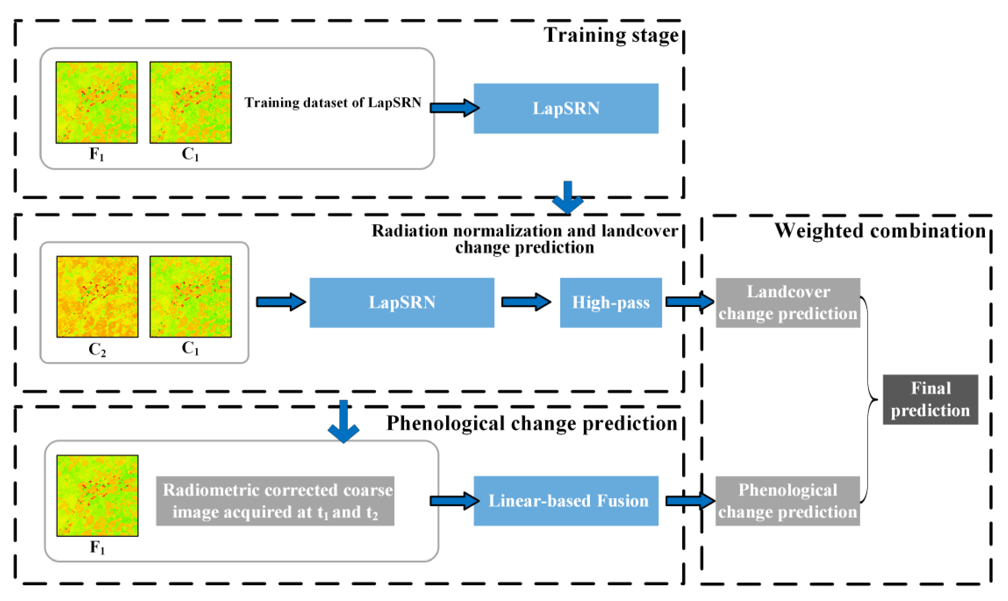
To validate the effectiveness of the HDLSFM, four experiments were conducted using three popular STF methods, namely STARFM, FSDAF, and Fit-FC, which also use one fine–coarse image pair as an input.

2. Methods

Differently from existing DL-based STF methods that need at least two pairs of fine–coarse images [42,48,53,54,55], HDLSFM requires minimal input data, i.e., a known fine $\left(F_1\right)$ and a coarse $\left(C_1\right)$ image at a base date ($t_1)$, and a coarse image $(C_2)$ at a prediction date ($t_2)$, to generate a robust target fine image ($F_2)$ containing both PC and LC information. This is achieved through a hybrid framework consisting of a nonlinear DL-based relative radiometric normalization that alleviates radiation differences, a DL-based SR algorithm for LC prediction, and linear-based fusion for PC prediction.

The flowchart of the HDLSFM for the prediction of $F_2$ is shown in Figure 1. In the first step, the radiation difference is alleviated through nonlinear DL-based relative radiometric normalization, followed by LC prediction using DL-based SR. The parameters of the DL-based nonlinear relative radiometric normalization and SR are learned simultaneously using a deep Laplacian pyramid SR network (LapSRN) [56]. In the second step, based on the corrected radiometric coarse images at the base date ($t_1$) and the prediction date ($t_2$), PC prediction is realized through linear-based fusion. Lastly, the final prediction is obtained through a weighted combination of PC and LC predictions using a sliding window. A detailed description of each step of HDLSFM is given below.

2.1. Radiation Normalization and Landcover Change Prediction

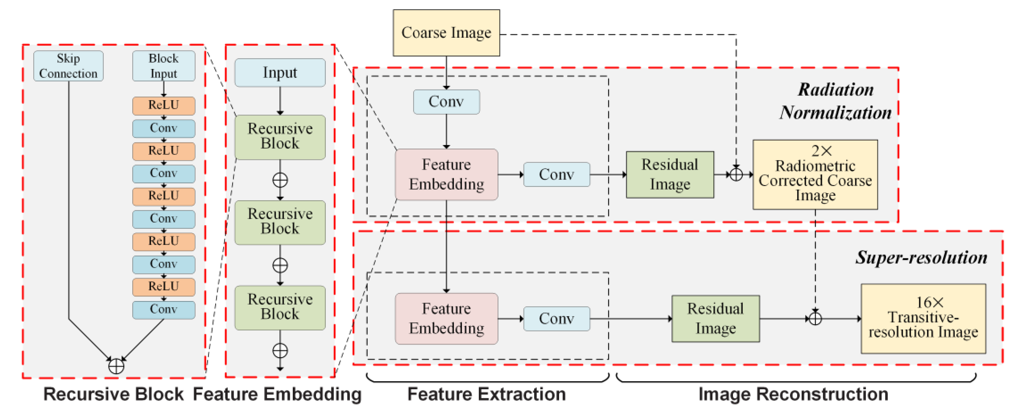
2.1.1. Radiation Normalization

STF methods assume that the radiation properties of fine and coarse images are similar. For this reason, i.e., due to their similar bandwidth and radiation, Landsat and MODIS images are widely used in STF. However, radiation differences between fine and coarse images are common, and are the primary sources of fusion errors in STF methods [12], limiting the application to other types of satellite images. The popular hybrid STF method, FSDAF, is based on the assumption that PC prediction $F_2^{\mathrm{PC}}\left(x_0,y_0,B\right)$ in band B for a pixel centered at $\left(x_0,y_0\right)$ can be obtained by adding a fine increment, $\mathsf{\Delta }F\left(c,B\right)$, to the known fine image, $F_1\left(x_0,y_0,B\right)$. This is expressed as:

$${\widehat{F}}_2^{\mathrm{PC}}\left(x_0,y_0,B\right)=F_1\left(x_0,y_0,B\right)+\mathsf{\Delta }F\left(c,B\right)$$

(1)

The fine increment, $\mathsf{\Delta }F\left(c,B\right)$, can be obtained using the spectral unmixing method as follows:

$$\mathsf{\Delta }C\left(x_0,y_0,B\right)={\displaystyle \sum }_{c=1}^l{f}_c\left(x_0,y_0\right)\times \mathsf{\Delta }F\left(c,B\right)$$

(2)

where $f_c\left(x,y\right)$ denotes the class fractions belonging to class c in a coarse image. It is obvious that $\mathsf{\Delta }F$ is dependent on the temporal change of coarse image $\mathsf{\Delta }C$, which means that Equation (1) may not be applicable when there is an obvious radiation difference between $\mathsf{\Delta }C$ and $\mathsf{\Delta }F$, which would introduce errors. These errors can be expressed using Equation (3), assuming that the radiation between fine and coarse image can be represented using a simple linear regression equation, such as Equation (4) [43].

$$∆{\widehat{F}}_{FSDAF}^R=\sum {\widehat{W}}_i\left(\alpha -1\right)\left(C_{2i}-C_{1i}\right)$$

(3)

$${\mathrm{C}}^{\prime }=\alpha C+\beta$$

(4)

where $C_{2i}$ and $C_{1i}$ are the ith similar pixel of the coarse image at the prediction date ($t_2$) and the base date ($t_1)$, ${\widehat{W}}_i$ is the weight value of the ith similar pixel, $C^{\prime }$ and $C$ are the pixel values (e.g., NDVI) of the fine and coarse image, respectively, and $\alpha$ and $\beta$ are the regression coefficients.

The popular weighting function-based STF method, Fit-FC, assumes that the temporal change between two coarse images ($C_1$ and $C_2$) is linear and predicts the target fine image, $F_2\left(x,y\right)$, by applying this linear relationship to the known fine image, $F_1$:

$$F_2\left(x,y\right)={\widehat{W}}_i\left(\widehat{a}\times F_1\left(x_i,y_i\right)+\widehat{b}+r\left(x_i,y_i\right)\right)$$

(5)

where $\widehat{a}$ and $\widehat{b}$ are the regression coefficients between $C_1$ and $C_2$, and $r\left(x_i,y_i\right)$ is the down-scaled residual.

Similarly, a fusion error, $∆{\widehat{F}}_{F\mathrm{it}-\mathrm{FC}}^R$, may be present if a radiation difference between fine and coarse image exists. This can be expressed as [43]:

$$∆{\widehat{F}}_{F\mathrm{it}-\mathrm{FC}}^R=\sum {\widehat{W}}_i(\left(\alpha -1\right)\left(C_{2i}-\widehat{a}{C}_{1i}\right)+\left(1-\widehat{a}\right)\beta )$$

(6)

It is thus critical to alleviate the radiation difference between fine and coarse images to achieve robust fusion, as well as to widen the applicability of the STF method to other types of satellite image. A common strategy is to utilize a relative radiometric normalization, which builds a simple linear regression between the fine and coarse images, assuming that this is a suitable model of the radiation difference [12,57]. However, it may not be suitable when the relationship between fine and coarse images is complex and nonlinear [10,43,58,59]. In this paper, a nonlinear DL-based relative radiometric normalization is proposed to alleviate the negative impact of radiation differences by formulating a nonlinear mapping between the fine and coarse image. In particular, the known fine image ($F_1$) is first aggregated to reduce its spatial resolution by approximately two times that of the coarse image, followed by the formulation of a nonlinear mapping ($f_1$) between this aggregated fine image ($F_1{}^{\mathrm{down}}$) and the coarse image ($C_1$) (Equation (7)).

$${\mathsf{\Phi }}_1=\mathrm{argmin}\mathcal{L}\left(f_1\left(C_1,\theta \right),F_1{}^{\mathrm{down}}\right)$$

(7)

The mapping parameter (${\mathsf{\Phi }}_1$) can be learned by the DL-based SR method, leveraging its capacity for formulating nonlinear mappings. Then, using the learned nonlinear mapping, $f_1$, the radiometrically corrected coarse image ($C_1^{\mathrm{RC}}$ and $C_2^{\mathrm{RC}}$) acquired at $t_1$ and $t_2$ can be obtained using:

$$C_1^{\mathrm{RC}}=f_1\left(C_1,{\mathsf{\Phi }}_1\right)$$

(8)

$$C_2^{\mathrm{RC}}=f_1\left(C_2,{\mathsf{\Phi }}_1\right)$$

(9)

Note that an aggregation step before the nonlinear mapping formulation is necessary, since a direct establishment of the mapping between the original fine and coarse images may not be effective due to the significant magnification, and may introduce uncertainties [42,53]. Instead, by aggregating the spatial resolution of the fine image to reduce the magnification, the reliability of the nonlinear mapping is improved. Moreover, since the spatial resolution of the output of the nonlinear-based relative radiometric normalization is improved to two times that of the original coarse image, $C_1^{\mathrm{RC}}$ and $C_2^{\mathrm{RC}}$ have more spatial detail, which is vital for PC prediction in areas with high heterogeneity (further explanation is provided in Section 2.2).

2.1.2. Landcover Change Prediction

An accurate prediction of LC is essential for STF performance. The coarse image ($C_2$) contains blurred LC information, which is vital, and complementary information for LC prediction. However, this information is incomplete due to the limited spatial resolution. In order to convert the spatial resolution of image ($C_2$) from low to high, spatial interpolation, such as thin plate spline interpolation, has been widely utilized in STF methods [12,44]. In this paper, the DL-based SR method is used to retain the complementary LC information, which is considered to be more beneficial for accurate LC prediction [36], and underpins a higher generalization ability because of the introduction of prior information [53,55]. According to the core of the DL-based SR method, the nonlinear mapping between $C_1^{\mathrm{RC}}$ and $F_1$ is formulated as:

$${\mathsf{\Phi }}_2=\mathrm{argmin}\mathcal{L}\left(f_2\left(C_1^{\mathrm{RC}},\theta \right),F_1\right)$$

(10)

Using the learned mapping ($f_2)$, a transitive-resolution image ($F_2^{\mathrm{Tran}}$) can be obtained by taking $C_2^{\mathrm{RC}}$ as the input (Equation (11)).

$$F_2^{\mathrm{Tran}}=f_2\left(C_2^{\mathrm{RC}},{\mathsf{\Phi }}_2\right)$$

(11)

Although the transitive-resolution image ($F_2^{\mathrm{Tran}}$) generated by the DL-based SR method has a spatial resolution close to that of the fine image, due to the significantly higher magnification factor of the STF compared to that of the single-image SR, $F_2^{\mathrm{Tran}}$ can have a smoothing effect. In order to reconstruct the spatial detail of $F_2^{\mathrm{Tran}}$ further, and obtain a more accurate LC prediction (${\widehat{F}}_2^{\mathrm{LC}}$), a high-pass modulation (Equation (12)) is applied by introducing the spatial detail information, expressed as $F_1-F_1^{\mathrm{Tran}}$, to the transitive-resolution image ($F_2^{\mathrm{Tran}})$.

$${\widehat{F}}_2^{\mathrm{LC}}=F_2^{\mathrm{Tran}}+g_b\left(F_1-F_1^{\mathrm{Tran}}\right)$$

(12)

where $g_b$ represents the injection gain that controls the spatial detail information introduction degree. This gain is locally optimized via a least square fitting in nonoverlapping zones [60], and is given by:

$$g_b=\frac{\mathrm{cov}\left(F_1^{\mathrm{Tran}},F_2^{\mathrm{Tran}}\right)}{\mathrm{var}\left(F_1^{\mathrm{Tran}}\right)}$$

(13)

where $\mathrm{cov}\left(F_1^{\mathrm{Tran}},F_2^{\mathrm{Tran}}\right)$ denotes the covariance between $F_1^{\mathrm{Tran}}$ and $F_2^{\mathrm{Tran}}$, while $\mathrm{var}\left(F_1^{\mathrm{Tran}}\right)$ denotes the variance of $F_1^{\mathrm{Tran}}$. Further explanation of the high-pass modulation is given in Section 5.2.

2.1.3. Integration of Radiation Normalization and Landcover Change Prediction

It is a common practice to learn the network parameters of mappings $f_1$ and $f_2$ by formulating two independent networks. However, these multiple steps are tedious. Besides, since the output of $f_1$, i.e., $C_2^{\mathrm{RC}}$, is regarded as the input of mapping ($f_2$) for prediction, the uncertainty of mapping ($f_1$) can be accumulated and exacerbated by $f_2$. Therefore, to simplify the steps and to mitigate the uncertainty accumulation, LapSRN is used to learn the network parameters of mappings $f_1$ and $f_2$ simultaneously. The original LapSRN consisted of multiple levels, each of which could up-sample the input by a scale of two using the feature extraction and image reconstruction parts. In this way, LapSRN can achieve SR with high magnification. In this paper, a two-level LapSRN is constructed, where the first level is utilized for radiation normalization, and the second to conduct SR. The architecture of the LapSRN used in HDLSFM is shown in Figure 2.

Similarly to the original LapSRN, each level of the LapSRN in HDLSFM consists of a feature extraction part, and an image reconstruction part. The feature extraction part includes a feature embedding sub-network and a residual model. A convolutional layer is added to the first level to transform the coarse image into high-dimensional nonlinear feature maps, followed by the feature embedding sub-network. The feature embedding sub-network is composed of five recursive blocks, each containing five distinct convolutional layers. The extracted features are not utilized to reconstruct an image but are forwarded to the second level. This strategy can reduce the cumulative uncertainty effectively. The reconstructed image is generated by combining the input image of each level with the reconstructed residual image. Each convolutional layer in the LapSRN contains 32 filters of size 3 × 3.

In each level of the original LapSRN, the input image is up-sampled by a scale of two using a transposed convolutional layer, which means that for SR with a scale of eight, three levels are required. However, the magnification factor of the STF method is large, meaning that more levels are required, which further increases computational cost. Therefore, in this paper the input coarse images were directly up-sampled to the same scale as the fine images using a nearest-neighbor interpolation algorithm before being fed to the network instead of achieving 2 $\times$ SR using the transposed convolutional layer in each level. In this way, different levels achieve different SR multiples.

In the training stage, the input is the coarse image ($C_1$) and the output of the two levels are the aggregated fine image $F_1{}^{\mathrm{down}}$ and $F_1$, respectively. To learn the parameters of LapSRN, the combination of the loss functions of the two levels is minimized, which is expressed as:

$${\mathcal{L}}_S\left(y,\widehat{y};\theta \right)=\frac{1}{\widehat{N}}{\displaystyle \sum }_{i^{\prime }=1}^{\widehat{N}}{\displaystyle \sum }_{l=1}^2\rho \left(y_l^{i^{\prime }}-{\widehat{y}}_l^{i^{\prime }}\right)$$

(14)

where $y$ represents the label of the two levels, i.e., $F_1{}^{\mathrm{down}}$ and $F_1$, $\widehat{y}$ denotes the output of the learned mapping, $\theta$ denotes the mapping parameter, $\rho$ stands for the Charbonnier penalty function, and $\widehat{N}$ is the number of training samples. The detailed parameter setup for training the LapSRN can be found in the Appendix A. In the prediction stage, using the learned LapSRN, the radiometric corrected coarse images and transitive-resolution images acquired at date $t_1$ and $t_2$, i.e., $C_1^{\mathrm{RC}}$, $F_1^{\mathrm{Tran}}$, and $C_2^{\mathrm{RC}}$, $F_2^{\mathrm{Tran}}$, respectively, can be obtained by taking $C_1$ and $C_2$ as the input. Then, the LC prediction (${\widehat{F}}_2^{\mathrm{LC}}$) can be obtained using Equations (12) and (13).

2.2. Linear-Based Fusion for Phenological Prediction

Although using the LapSRN coupled with high-pass modulation can reconstruct the spatial details of $C_2$ so as to achieve LC prediction, since no temporal change information is utilized, the PC prediction performance will still be limited. Therefore, a linear-based fusion is proposed to improve the PC prediction performance.

Suppose that the land surface temporal change of a coarse image between $t_1$ and $t_2$ can be described using the following linear regression model:

$$C_2\left(x_0,y_0,B,t_2\right)=w\left(x_0,y_0,B,∆t\right)\times C_1\left(x_0,y_0,B,t_1\right)+b\left(x_0,y_0,B,∆t\right)+R\left(x_0,y_0,B,∆t\right)$$

(15)

where $∆t$ denotes the time interval between $t_1$ and $t_2$. The local regression coefficients $w\left(x_0,y_0,B,∆t\right)$ and $b\left(x_0,y_0,B,∆t\right)$ can be estimated using the least square method in a sliding window in band B centered at $\left(x_0,y_0\right)$, while $R\left(x_0,y_0,B,∆t\right)$ is the residual.

Then, the target PC prediction (${\widehat{F}}_2^{\mathrm{PC}}$) can be generated through the application of the local regression coefficients and residual to $F_1$:

$${\widehat{F}}_2^{\mathrm{PC}}\left(x_0,y_0,B,t_2\right)=w\left(x_0,y_0,B,∆t\right)\times F_1\left(x_0,y_0,B,t_1\right)+b\left(x_0,y_0,B,∆t\right)+R\left(x_0,y_0,B,∆t\right)$$

(16)

However, Equations (15) and (16) may not be effective in the following aspects:

(1) As described in Section 2.1.1, the radiation difference between the fine and coarse images can affect the fusion performance adversely.

(2) The spatial resolutions of regression coefficients $w\left(x_0,y_0,B,∆t\right)$ and $b\left(x_0,y_0,B,∆t\right)$ are the same as that of the coarse image, which is significantly different from that of $F_1\left(x_0,y_0,B,t_1\right)$. This spatial resolution inconsistency can cause blocky artifacts.

(3) An assumption of Equation (16) is that the temporal changes of the fine and coarse images are consistent, which is valid only for homogeneous pixels (hereafter, “homogenous pixel assumption”).

To mitigate the uncertainty caused by the radiation difference, the original coarse images ($C_1$ and $C_2$) in Equation (15) are replaced by the radiometrically corrected coarse images acquired at $t_1$ and $t_2$ ($C_1^{\mathrm{RC}}$ and $C_2^{\mathrm{RC}}$) that are obtained by the LapSRN. The aim is to estimate the local regression coefficients, $w^{\prime }\left(x_0,y_0,B,∆t\right)$ and $b^{\prime }\left(x_0,y_0,B,∆t\right)$, which are expressed as Equation (17). The reason for this replacement is that the radiation normalization can move $\alpha$ and $\beta$ in Equation (6) closer to 1 and 0, respectively, resulting in $∆{\widehat{F}}_{F\mathrm{it}-\mathrm{FC}}^R$ being closer to 0; in other words, smaller fusion errors will be caused by radiation difference.

$$C_2^{\mathrm{RC}}\left(x_0,y_0,B,t_2\right)=w^{\prime }\left(x_0,y_0,B,∆t\right)\times C_1^{\mathrm{RC}}\left(x_0,y_0,B,t_1\right)+b^{\prime }\left(x_0,y_0,B,∆t\right)+R\left(x_0,y_0,B,∆t\right)$$

(17)

Then, an initial PC prediction, $F_2^{\mathrm{PC}}{}^{\prime }\left(x_0,y_0,B,t_2\right)$, can be obtained by applying the regression coefficients, $w^{\prime }\left(x_0,y_0,B,∆t\right)$ and $b^{\prime }\left(x_0,y_0,B,∆t\right)$, and the residual, $R\left(x_0,y_0,B,∆t\right)$, to $F_1\left(x_0,y_0,B,t_1\right)$ as follows:

$$F_2^{\mathrm{PC}}{}^{\prime }\left(x_0,y_0,B,t_2\right)=w^{\prime }\left(x_0,y_0,B,∆t\right)\times F_1\left(x_0,y_0,B,t_1\right)+b^{\prime }\left(x_0,y_0,B,∆t\right)+R\left(x_0,y_0,B,∆t\right)$$

(18)

Note that since the radiometrically corrected coarse images $C_1^{\mathrm{RC}}$ and $C_2^{\mathrm{RC}}$ have higher spatial resolutions than the original coarse images, the spatial resolutions of $w^{\prime }\left(x_0,y_0,B,∆t\right)$ and $b^{\prime }\left(x_0,y_0,B,∆t\right)$ are closer to that of $F_1\left(x_0,y_0,B,t_1\right)$ compared to that of the original regression coefficient. In this manner, the blocky artifacts are alleviated.

For the fusion errors caused by the homogenous pixel assumption, we utilized a strategy similar to STARFM, ESTARFM, and FSDAF, which use additional neighboring pixels in the sliding window for achieving a more robust prediction. In particular, pixels $F_1\left(x_{l^{\prime }},y_{l^{\prime }},\mathrm{B}\right)$ that are within the sliding window and have small spectral differences from the fine target pixel, $F_1\left(x_0,y_0,\mathrm{B}\right)$, i.e., those that satisfy Equation (19), are selected as similar pixels.

$$\left|F_1\left(x_{l^{\prime }},y_{l^{\prime }},\mathrm{B}\right)-F_1\left(x_0,y_0,\mathrm{B}\right)\right|\le \mathsf{\sigma }\left(B\right)\times 2/m$$

(19)

where $\sigma \left(B\right)$ denotes the standard deviation of band B of $F_1$, and $m$ represents the number of classes, which is set to four in this paper. Then, the final PC prediction (${\widehat{F}}_2^{\mathrm{PC}}$) of each central pixel, ${\widehat{F}}_2^{\mathrm{PC}}\left(x_0,y_0,B\right)$, is obtained using a weighted combination of selected similar pixels in the sliding window of the initial PC prediction, $F_2^{\mathrm{PC}}{}^{\prime }$:

$${\widehat{F}}_2^{\mathrm{PC}}\left(x_0,y_0,B\right)={\displaystyle \sum }_{i=1}^{N}W\left(x_i,y_i\right)F_2^{\mathrm{PC}}{}^{\prime }\left(x_i,y_i,B\right)$$

(20)

The weight of each similar pixel, $W\left(x_i,y_i\right)$, in the sliding window is determined by:

$$W\left(x_i,y_i\right)=\left(1/D\left(x_i,y_i\right)\right)/{\displaystyle \sum }_{i=1}^{N^{\prime }}\left(1/D\left(x_i,y_i\right)\right)$$

(21)

where N′ denotes the number of selected pixels in the sliding window, and $D\left(x_i,y_i\right)$ is defined as:

$$D\left(x_i,y_i\right)=1+\sqrt{{\left(x_i-x_0\right)}^2+{\left(y_i-y_0\right)}^2}/\left(\widehat{w}/2\right)$$

(22)

where $\widehat{w}$ denotes the sliding window size, which was set to 50 in this paper. A further explanation of the prediction performance’s sensitivity to $\widehat{w}$ is given in Section 5.1.

2.3. Combination of Linear- and Deep Learning-Based STF

${\widehat{F}}_2^{\mathrm{LC}}$ and ${\widehat{F}}_2^{\mathrm{PC}}$ focus on the LC and PC predictions, respectively. A weighted combination method is employed to synthesize ${\widehat{F}}_2^{\mathrm{LC}}$ and ${\widehat{F}}_2^{\mathrm{PC}}$ to obtain a robust final prediction ${\widehat{F}}_2$, which is given by:

$${\widehat{F}}_2\left(x_0,y_0,B,t_2\right)=p^{\mathrm{LC}}\left(x_0,y_0,B,t_2\right){\widehat{F}}_2^{\mathrm{LC}}\left(x_0,y_0,B,t_2\right)+p^{\mathrm{PC}}\left(x_0,y_0,B,t_2\right){\widehat{F}}_2^{\mathrm{PC}}\left(x_0,y_0,B,t_2\right)$$

(23)

The weight values $p^{\mathrm{LC}}$ and $p^{\mathrm{PC}}$ are determined using the absolute difference between ${\widehat{F}}_2^{\mathrm{LC}}$ and ${\widehat{F}}_2^{\mathrm{PC}}$ and $C_2$ in a 3 × 3 sliding window as follows:

$$p^{\mathrm{PC}}\left(x_0,y_0\right)=\frac{{\sigma }^{\mathrm{PC}}\left(x_0,y_0\right)}{{\sigma }^{\mathrm{PC}}\left(x_0,y_0\right)+{\sigma }^{\mathrm{LC}}\left(x_0,y_0\right)}$$

(24)

$$p^{\mathrm{LC}}\left(x_0,y_0\right)=\frac{{\sigma }^{\mathrm{LC}}\left(x_0,y_0\right)}{{\sigma }^{\mathrm{PC}}\left(x_0,y_0\right)+{\sigma }^{\mathrm{LC}}\left(x_0,y_0\right)}$$

(25)

where ${\sigma }^{\mathrm{PC}}\left(x_0,y_0\right)$ and ${\sigma }^{\mathrm{LC}}\left(x_0,y_0\right)$ are obtained by:

$${\sigma }^{\mathrm{PC}}\left(x_0,y_0\right)=\frac{1}{{{\displaystyle \sum }}_{j=1}^9\left|{\widehat{F}}_2^{\mathrm{PC},j}\left(x_0,y_0\right)-C_2{}^j\left(x_0,y_0\right)\right|}$$

(26)

$${\sigma }^{\mathrm{LC}}\left(x_0,y_0\right)=\frac{1}{{{\displaystyle \sum }}_{j=1}^9\left|{\widehat{F}}_2^{\mathrm{LC},j}\left(x_0,y_0\right)-C_2{}^j\left(x_0,y_0\right)\right|}$$

(27)

where ${\widehat{F}}_2^{\mathrm{LC},j}\left(x_0,y_0\right)$ and ${\widehat{F}}_2^{\mathrm{PC},j}\left(x_0,y_0\right)$ denote the jth pixels of the LC and PC predictions in a 3 × 3 sliding window centered at $\left(x_0,y_0\right)$, while $C_2{}^j\left(x_0,y_0\right)$ represents the corresponding pixel of $C_2$. Further validation of the weighted combination method is given in Section 5.2.

3. Experimental Setup and Datasets

3.1. Experimental Setup

Four experiments were performed to test the effectiveness of HDLSFM from the following four perspectives: (1) LC prediction, (2) PC prediction, (3) generation of fused time-series data, and (4) application of HDLSFM to other types of satellite images. A detailed description of the experimental setup and dataset of each experiment is given in the following.

3.1.1. Experiment I: Effectiveness of HDLSFM in Landcover Change Prediction

The study site of Experiment I was the Lower Gwydir Catchment (LGC), located in northern New South Wales, where a large flood in mid-December 2004 led to significant LC. It is thus suitable for testing the effectiveness of HDLSFM in LC prediction. The dataset of Experiment I was the same as the one used by Emelyanova et al. [61]. A MODIS and Landsat 5 TM image pair (3200 × 2720 pixels), acquired on 26 November 2004, and a MODIS image acquired on 12 December 2004, were used to predict the fine Landsat image acquired on 12 December 2004, as shown in Figure 3.

3.1.2. Experiment II: Effectiveness of HDLSFM in Phenological Change Prediction

The study site of Experiment II was a heterogeneous rain-fed agricultural area in central Iowa (CI), USA. This study site was chosen to test the effectiveness of HDLSFM in PC prediction. The dataset of this experiment was the same as the one used by Jia et al. [53]. A MODIS and Landsat ETM+ image pair (4500 × 4500 pixels) acquired on 14 May 2002, along with a MODIS image acquired on 2 July 2002, were utilized to predict the Landsat image acquired on 2 July 2002, as shown in Figure 4.

3.1.3. Experiment III: Effectiveness of HDLSFM in Generating Fused Time-Series Data

The study site of Experiment III was the Coleambally irrigation area (CIA), southern New South Wales, Australia. This area has a spatially heterogeneous landscape and rapid PC. Seventeen cloud-free Landsat ETM+ and MODIS (MOD09GA) pairs were available for this study site, covering the 2001–2002 summer growing season. The details of this study site’s dataset can be found in [61].

Under ideal conditions, the fine and coarse image pair dated closest to the prediction image would be utilized for generating the fused time-series data. That is, the shorter the time interval, the lower the difficulty of the STF will be [62]. However, the number of available fine images is usually limited, resulting in irregular time intervals.

Experiment III was thus designed to test the effectiveness of HDLSFM in using a limited number of fine–coarse image pairs with irregular time intervals to generate fused time-series data. Referring to [48], three Landsat ETM+ and MODIS MOD09GA pairs acquired on 8 October 2001, 4 December 2001, and 11 April 2002, along with the other available MOD09GA images were used to predict the other fourteen Landsat images (

Table 1. Date and function of Landsat images in Experiment III.

Known Fine Image Date	Prediction Date
8 October 2001	1st	17 October 2001
	2nd	2 November 2001
4 December 2001	3rd	9 November 2001
	4th	25 November 2001
	5th	5 January 2002
	6th	12 January 2002
11 April 2002	7th	13 February 2002
	8th	22 February 2002
	9th	10 March 2002
	10th	17 March 2002
	11th	2 April 2002
	12th	18 April 2002
	13th	27 April 2002
	14th	4 May 2002

). In this case, the time interval between the base date and the prediction date ranged from 9 days to 57 days, which can be considered as suitable for testing the robustness of the HDLSFM to time interval variation.

3.1.4. Experiment IV: Effectiveness of HDLSFM on Other Types of Satellite Images

In order to test the effectiveness of HDLSFM on other types of satellite images, in Experiment IV the VIIRS Surface Reflectance Daily product VNP09GA and Landsat 8 OLI were used as the coarse and fine images, respectively. Since the bands I1, I2, and I3 of a VIIRS image at a 500m spatial resolution have the most similar radiation features to bands 4, 5, and 6 of a Landsat OLI, these bands were used to perform STF.

A complex cropland area, located in the southwest of Kansas State (SWK), USA, was selected as the study site. This study site is covered by one Landsat OLI scene with a path/row of 30/34. Five cloud-free Landsat OLI images (3500 × 2500 pixels) were available for this study site. As shown in

Table 2. Identifications and functions of Landsat images in Experiment IV.

Sensor Identification	Function
LC080300342019060201T1-SC20200325041150	Known image at base date
LC080300342019072001T1-SC20200325041156	Prediction
LC080300342019090601T1-SC20200325041203	Prediction
LC080300342019092201T1-SC20200325041142	Prediction
LC080300342019100801T1-SC20200325041147	Prediction

, the Landsat OLI and VNP09GA acquired on 2 June 2019, and the VNP09GA images obtained on 20 July, 6 September, 22 September, and 8 October in 2019, were regarded as the known images to predict the Landsat images. The actual Landsat images obtained on these dates were utilized to evaluate the fusion performance.

3.2. Comparison and Evaluation Strategy

In order to evaluate the performance of HDLSFM, three widely-used STF methods, namely STARFM, FSDAF, and Fit-FC, were used as benchmark methods; all use one fine–coarse image pair as input. Note that although revisions of FSDAF, i.e., IFSDAF, SFSDAF, and FSDAF 2.0 have been proposed, the framework of these hybrid STF methods is basically consistent with the original FSDAF. Moreover, FSDAF has been widely used [63,64,65,66], suggesting its effectiveness and representativeness. We thus used FSDAF as the representative method of the hybrid STF methods.

Fusion performance was assessed quantitatively using six evaluation indices: root mean square error (RMSE), structural similarity (SSIM) [67], universal image quality index (UIQI) [68], correlation coefficient (CC), erreur relative global adimensionnelle de synthèse (ERGAS) [69], and the spectral angle mapper (SAM) [70]. The ideal values of RMSE, CC, SSIM, and UIQI are 0, 1, 1, and 1, respectively. The closer the SAM and ERGAS are to zero, the lower the uncertainty of the predictions. A description of the indices used is not provided in this work due to space limitations; for further information, please refer to [53].

4. Experimental Results

4.1. Experiment I

The visual effects of the predictions of HDLSFM and the benchmark methods for the LGC site are shown in Figure 5. It can be seen that STARFM and Fit-FC exhibited the worse visual artifacts, with blurry spatial details compared to the other fusion methods, especially in the inundated area. The worse quantitative results of the two STF methods, both in the complete LGC site (Figure 6) and the sub area (

Table 3. Prediction results for the sub area of the LGC site. Bold values indicate best results.

Index	Band	STARFM	FSDAF	Fit-FC	HDLSFM
RMSE (root mean square error)	Band 1	0.0185	0.0160	0.0193	0.0163
	Band 2	0.0234	0.0223	0.0249	0.0233
	Band 3	0.0298	0.0262	0.0297	0.0264
	Band 4	0.0493	0.0358	0.0397	0.0353
	Band 5	0.2684	0.0630	0.0652	0.0584
	Band 7	0.3117	0.0536	0.0546	0.0457
SSIM (structural similarity)	Band 1	0.8895	0.9041	0.8702	0.9096
	Band 2	0.8447	0.8624	0.8255	0.8634
	Band 3	0.8077	0.8344	0.7899	0.8385
	Band 4	0.7142	0.7505	0.6997	0.7604
	Band 5	0.3856	0.4993	0.4456	0.5014
	Band 7	0.3748	0.5544	0.5381	0.5743
UIQI (universal image quality index)	Band 1	0.9355	0.9375	0.9058	0.9388
	Band 2	0.9424	0.9437	0.9352	0.9430
	Band 3	0.9426	0.9456	0.9373	0.9487
	Band 4	0.9326	0.9382	0.9326	0.9420
	Band 5	0.6452	0.6983	0.7349	0.7487
	Band 7	0.5297	0.5834	0.7031	0.7121
CC (correlation coefficient)	Band 1	0.6120	0.6958	0.6356	0.6988
	Band 2	0.7010	0.7308	0.6610	0.7127
	Band 3	0.6551	0.7353	0.6453	0.7348
	Band 4	0.6541	0.8224	0.7540	0.8190
	Band 5	0.4170	0.7421	0.6310	0.7527
	Band 7	0.3789	0.7062	0.5213	0.7386
SAM (spectral angle mapper)		20.4060	13.0858	13.8030	11.7314
ERGAS (erreur relative global adimensionnelle de synthèse)		24.1511	2.8994	2.4629	2.2766

), confirmed the unsuitability of these methods for the prediction of significant LC, which is mainly due to the insufficiency of the linear assumption in LC prediction. Compared to STARFM and Fit-FC, FSDAF achieved better fusion performance in LC prediction. FSDAF’s clearer spatial variation, complete boundary of the inundated area, and the comparatively good quantitative results in the sub area suggest its effectiveness in LC prediction. HDLSFM generated a similar visual effect to FSDAF, with complete spatial detail of the LC area. This is attributed to the combined use of DL-based SR and high-pass modulation. Moreover, compared to FSDAF, HDLSFM showed better quantitative performance in the whole LGC site in almost all the six bands (Figure 6), as well as in the sub area of the LGC site (Table 3).

For the whole LGC site, the mean RMSE of HDLSFM was 0.0329, with a decrease of 0.0616, 0.0021, and 0.0016 when compared to STARFM, FSDAF, and Fit-FC. The mean SSIM of HDLSFM was 0.7619, with gains of 0.0732, 0.0152, and 0.0215 over those of STARFM, FSDAF, and Fit-FC. HDLSFM achieved the best mean UIQI and CC (i.e., 0.8989 and 0.7573) for the whole LGC site, with an increase of 0.0029 and 0.0048 over those of FSDAF, and with an increase of 0.0086 and 0.0327 over those of Fit-FC. HDLSFM also achieved a significant improvement in SAM, i.e., 10.4542 with an improvement of 60.90%, 13.74%, and 9.56% over STARFM, FSDAF, and Fit-FC. The above results confirm the effectiveness and the superiority of the HDLSFM in LC prediction.

4.2. Experiment II

A visual comparison of the predictions obtained by the HDLSFM and the three benchmark methods of the CI site is shown in Figure 7. The rapid PC between the known Landsat image at the base date (Figure 7c) and the actual Landsat image (Figure 7a), as well as high spatial heterogeneity, are indicative of the great difficulty we expected the STF to face. STARFM again yielded the worst fusion accuracy among all the STF methods (Figure 8) and a significant spectral deviation (Figure 7e), which demonstrates that it may not be suitable for areas with rapid PC and high spatial heterogeneity. Fit-FC suffered from smaller spectral deviation than STARFM (Figure 7g); however, its fusion result had blurry texture details, suggesting that although the Fit-FC can address rapid PC prediction, its applicability in heterogeneous areas may be limited. FSDAF, by comparison, provided the most complete spatial details (Figure 7f), indicating the advantage of the linear unmixing model in preserving spatial details in PC prediction. HDLSFM provided the best performance (Figure 8) regarding most of the evaluation indices. The mean RMSE of HDLSFM was 0.0339, with a decrease of 0.0638, 0.0051, and 0.0016 when compared to STARFM, FSDAF, and Fit-FC. The mean SSIM of HDLSFM was 0.6850, with an increase of 0.1266, 0.0389, and 0.080 over STARFM, FSDAF, and Fit-FC. The mean UIQI and CC of HDLSFM was 0.9468 and 0.5888, with an increase of 0.0242 and 0.0560 over those of FSDAF, and with an increase of 0.0074 and 0.0098 over those of Fit-FC. Similarly to Experiment I, HDLSFM achieved a significant improvement in SAM, i.e., 7.9944 with an increase of 65.02%, 21.26%, and 2.13% over STARFM, FSDAF, and Fit-FC. The above results verified the effectiveness of the HDLSFM in PC prediction.

However, the spatial effect of HDLSFM (Figure 7h) was a bit inferior to that of FSDAF (Figure 7f). The reason for this may lie in the fact that HDLSFM employs a DL-based SR method for the restoration of spatial details from the coarse image at the prediction date, whose performance is closely related to the number of fine–coarse image pairs. Therefore, when using a limited number of fine–coarse images, the fusion spatial details of HDLSFM may be lost in heterogeneous areas.

4.3. Experiment III

The quantitative assessment of the results of different STF methods for the CIA site is shown in Figure 9. In general, STARFM and Fit-FC had the worst fusion performance, which is probably due to their high sensitivity to time interval, indicating the weighting function-based STF methods’ ineffectiveness in the case of long time intervals. HDLSFM achieved the best fusion performance in almost all evaluation indices except SAM. The mean RMSE for all dates of HDLSFM was 0.0303, with a significant decrease of 0.0155 when compared to STARFM. The mean SSIM of HDLSFM was 0.8245, with an increase of 0.0381, 0.0045, and 0.0221 over those of STARFM, FSDAF, and Fit-FC. The mean UIQI of HDLSFM was 0.9550, with an increase of 0.0080, 0.0025, and 0.0055 when compared to STARFM, FSDAF, and Fit-FC. The mean CC of HDLSFM was 0.8206, with an increase of 0.1184, 0.0097, and 0.0329 over STARFM, FSDAF, and Fit-FC. The mean SAM of HDLSFM was 5.7320, with a decrease of 1.1216 and 0.5888 when compared to STARFM and Fit-FC, but it was slightly inferior to FSDAF. Nevertheless, the best fusion performance in almost all evaluation indices and the comparative performance in SAM verified the effectiveness of the HDLSFM in generating fused time-series data. Note that although the weighting function-based method employed in HDLSFM for PC prediction may also suffer from the uncertainties caused by long time intervals, these uncertainties are alleviated through the synthesis with LC prediction.

To further analyze the sensitivity of different STF methods to time interval, the visual effect (Figure 10) and the performance of the predictions of the different STF methods was compared on a sub-area of the CIA site on 13 February 2002 (

Table 4. Quantitative assessment of the prediction on 13 Feb 2002 of different STF methods in the sub-area of the CIA site. Bold values indicate best results.

Index	Band	STARFM	FSDAF	Fit-FC	HDLSFM
RMSE	band 1	0.0335	0.0194	0.0173	0.0156
	band 2	0.0280	0.0275	0.0235	0.0211
	band 3	0.0884	0.0438	0.0350	0.0343
	band 4	0.0547	0.0525	0.0508	0.0493
	band 5	0.0777	0.0610	0.0612	0.0561
	band 7	0.0825	0.0544	0.0514	0.0499
SSIM	band 1	0.8553	0.8446	0.8747	0.8884
	band 2	0.8087	0.7970	0.8381	0.8549
	band 3	0.6506	0.6612	0.7350	0.7502
	band 4	0.6299	0.6517	0.6886	0.6961
	band 5	0.5719	0.6149	0.6560	0.6592
	band 7	0.5706	0.6245	0.6597	0.6624
UIQI	band 1	0.8960	0.8705	0.8964	0.9155
	band 2	0.9260	0.9096	0.9294	0.9443
	band 3	0.8546	0.8497	0.8930	0.8996
	band 4	0.9642	0.9643	0.9653	0.9690
	band 5	0.9362	0.9444	0.9458	0.9544
	band 7	0.8929	0.8989	0.9151	0.9178
CC	band 1	0.3996	0.6186	0.6840	0.7413
	band 2	0.5326	0.5609	0.6503	0.7318
	band 3	0.3679	0.6097	0.7446	0.7604
	band 4	0.7515	0.7738	0.7870	0.8045
	band 5	0.6763	0.7888	0.7692	0.8090
	band 7	0.6691	0.8152	0.8226	0.8345
SAM		9.1292	8.0004	8.1169	7.5171
ERGAS		2.4817	1.5588	1.3590	1.2855

), since this prediction date had the largest time interval. As in the case of Figure 9, STARFM had the worst visual effect and fusion accuracy in the sub-area, which confirmed its high sensitivity to time interval. The fusion accuracy of FSDAF in the sub-area was worse than Fit-FC, which is slightly different from Figure 9. As shown in Figure 10, although FSDAF again had the most complete spatial details, large bias can be observed in areas with obvious PC. Fit-FC, by comparison, shows better fusion performance than FSDAF in the PC area; however, as in Experiment II (Figure 7), the lack of spatial details is a major limitation of Fit-FC. HDLSFM had the best fusion accuracy in the sub-area, as well as a good visual effect in the PC area, suggesting it is less sensitive to the time interval. Thus, it can provide a more robust prediction result than the other STF methods for a limited number of fine–coarse image pairs.

4.4. Experiment IV

Experiment IV was performed to determine whether STF is still effective when applied to other types of satellite images with more radiation differences than those between MODIS and Landsat. In this case, VIIRS and Landsat 8 OLI were used as the coarse and fine images, respectively. As shown in Figure 11, the linear correlation between VIIRS and OLI was significantly lower than that of MODIS, indicating larger radiation differences between OLI and VIIRS.

As shown in Figure 12, STARFM still yielded the worst fusion accuracy. FSDAF generated lower fusion accuracy than Fit-FC (Figure 12), as well as a more obvious bias in the prediction for all the dates (Figure 13), which was slightly different from the other experimental results presented in this paper. This is probably due to the fact that the linear unmixing method for obtaining the temporal change value at fine resolution is sensitive to radiation differences between fine and coarse images. In order to reduce these differences, FSDAF employs a simple linear regression-based radiometric normalization. However, this approach is not effective when the relationships between fine and coarse images are complex and nonlinear. As shown in Figure 11, compared to simple linear regression, the nonlinear-based relative radiometric normalization improved the correlation between fine and coarse images obviously, demonstrating its effectiveness in reducing the radiation difference. Fit-FC showed a better fusion performance than STARFM and FSDAF. Nevertheless, HDLSFM achieved a significant improvement in the average Average Absolute Difference (AAD) map, showing the least bias (Figure 13) in the predictions for all the dates, as well as the best fusion performance (Figure 12) on most of the evaluation indices compared to the three benchmark fusion methods. The mean RMSE for all dates for HDLSFM was 0.0621, with a significant improvement of 55.19%, 30.47%, and 9.94% when compared to STARFM, FSDAF, and Fit-FC. The mean SSIM of HDLSFM was 0.5826, with an increase of 0.1307, 0.0767, and 0.0071 over STARFM, FSDAF, and Fit-FC. The mean UIQI of HDLSFM was 0.9286, with an increase of 0.0416, 0.0521, and 0.0083 when compared to STARFM, FSDAF, and Fit-FC. The mean CC of HDLSFM was 0.4311 with a significant improvement of 42.80%, 21.74%, and 6.85% over STARFM, FSDAF, and Fit-FC. The mean SAM of HDLSFM was 7.2170, with a significant improvement of 47.85%, 38.00%, and 12.70% when compared to STARFM, FSDAF, and Fit-FC. The improvement in fusion accuracy is indicative of HDLSFM’s higher applicability to other types of satellite image.

5. Discussion

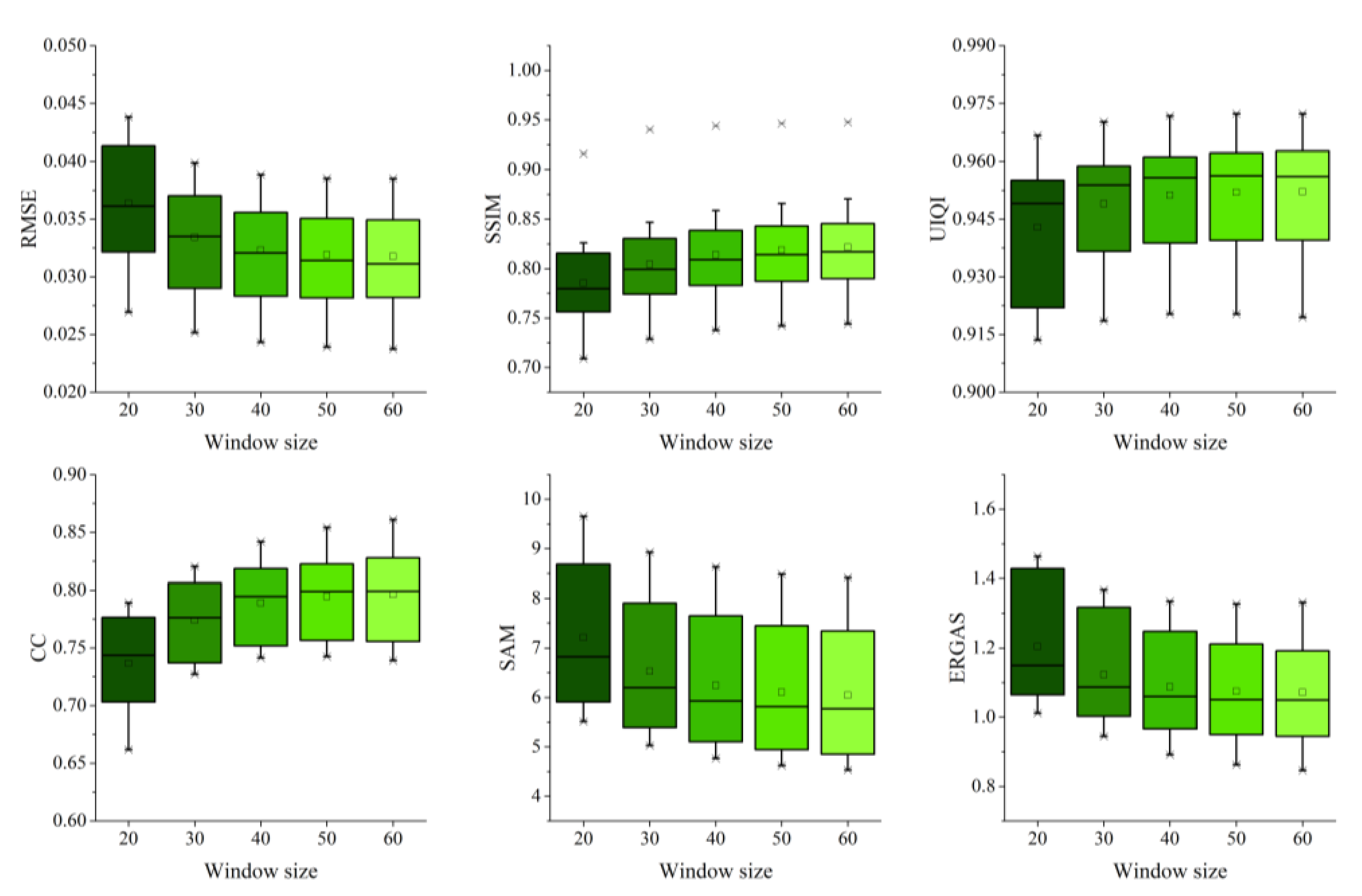
5.1. Prediction Performance Sensitivity to Moving Window Size

The moving window size ($\widehat{w})$ defines the number of pixels that are utilized to calculate the local regression coefficients, $a^{\prime }\left(x_0,y_0,B,∆t\right)$ and $b^{\prime }\left(x_0,y_0,B,∆t\right),$ and the number of similar pixels. The influence of the moving window size was analyzed using the CIA site. The experiment was performed on the same dataset as that in Table 1. As shown in Figure 14, in general, the fusion performance improves with the increase in the moving window size. When the window size exceeds 50, the fusion performance remains relatively stable. Since there is always a trade-off between the moving window size and computation time, based on the obtained results, the moving window size in this work was chosen to be 50.

5.2. High-Pass Modulation in Spatial Detail Reconstruction

The LC prediction performance of the HDLSFM depends on the performance of the DL-based SR method, which formulates the nonlinear mapping between fine and coarse images. However, due to the significantly larger magnification factor of the STF compared to that of single-image SR, their spatial details are incomplete. Thus, in order to recover the spatial details, high-pass modulation was employed, which is a common strategy in existing learning-based STF methods [48,52,71,72,73]. An alternative way is to introduce spatial details, described as the difference between known fine and coarse images $F_1-C_1$, into typical the SR mapping ($f$) between $C_3$ and $F_3$, as proposed by Jia [53]:

$$\mathsf{\Phi }=\mathrm{argmin}\mathcal{L}\left(f\left(C_3,F_1-C_1,\theta \right),F_3\right)$$

(28)

Compared to the high-pass modulation (Equation (12)), the essence of Equation (28) is to use DL to learn the injection gain (Equation (13)) automatically with a higher generalization ability. However, since the learning network parameter ($\mathsf{\Phi }$) requires two pairs of fine and coarse images, achieving an injection gain with a higher generalization ability comes with the cost of increasing the number of fine and coarse image pairs. Therefore, this approach is not suitable when there is only one known fine–coarse image pair. In order to reduce the requirement for the number of fine–coarse image pairs, while achieving high practicality, in the HDLSFM the injection gain is predefined instead of being automatically learned by the DL-based SR method. Although the generalization ability of the predefined-injection gain is lower than that of the automatically learned one, its relaxed requirement on the number of input images makes the HDLSFM highly practical.

5.3. Fusion of LC Prediction with PC Prediction

In HDLSFM, the LC and PC predictions are combined using the weighted combination method with a sliding window, constituting a sliding window-combination method. It should be noted that in IFSDAF [44], the final prediction is also obtained by combining two independent fused images using a weighted combination method, forming the constrained least squares (CLS)-combination, in which the weights are estimated via a constrained least squares method on the scale of the coarse images. In order to further test the effectiveness of the sliding window-combination method adopted in HDLSFM, a comparison of the fusion performance of the CLS-combination method and the sliding window-combination method for the LGC and CI sites was conducted. As shown in

Table 5. Quantitative results of the sliding window-combination (Com-1) and CLS-combination (Com-2) methods applied to the LGC and CI sites. Bold values indicate best results.

Index	Band	LGC Site		CI Site
		Com-1	Com-2	Com-1	Com-2
RMSE	Band 1	0.0137	0.0142	0.0143	0.0145
	Band 2	0.0195	0.0201	0.0169	0.0171
	Band 3	0.0242	0.0248	0.0259	0.0260
	Band 4	0.0381	0.0377	0.0498	0.0497
	Band 5	0.0569	0.0576	0.0479	0.0479
	Band 7	0.0451	0.0455	0.0483	0.0484
SSIM	Band 1	0.9258	0.9202	0.9098	0.9068
	Band 2	0.8828	0.8746	0.872	0.8693
	Band 3	0.8486	0.8391	0.7597	0.7561
	Band 4	0.7369	0.7377	0.5028	0.5029
	Band 5	0.5482	0.5465	0.5426	0.5422
	Band 7	0.6289	0.6227	0.5232	0.5226
UIQI	Band 1	0.9534	0.9506	0.9464	0.9438
	Band 2	0.9567	0.9544	0.9636	0.9629
	Band 3	0.9516	0.9492	0.9088	0.9073
	Band 4	0.9483	0.9488	0.9845	0.9845
	Band 5	0.8089	0.8065	0.9694	0.9694
	Band 7	0.7746	0.7704	0.9083	0.9087
CC	Band 1	0.7210	0.7016	0.6295	0.6186
	Band 2	0.7091	0.6917	0.6400	0.6299
	Band 3	0.7271	0.7128	0.5740	0.5672
	Band 4	0.8173	0.8199	0.6148	0.6149
	Band 5	0.7915	0.786	0.5644	0.5649
	Band 7	0.7777	0.7769	0.5099	0.5088
SAM		10.4542	10.7636	7.9944	8.018
ERGAS		1.8990	1.9349	1.5754	1.5824

, the sliding window-combination method generally achieved better fusion performance than the CLS-combination method for both sites.

Theoretically, the weights of both combination methods are estimated on the scale of the coarse images, which can easily cause a block effect due to the scale inconsistency between the coarse image and two independent fused images. In HDLSFM, in order to obtain a smoother fusion result, the weight measurement is based on a sliding window. The comparison of the visual effects of the two combination methods (Figure 15) verifies HDLSFM’s effectiveness, as more spatial details can be seen.

5.4. Comparison with Other DL-Based STF Methods

HDLSFM requires minimal input data, i.e., a known fine and a coarse image at a base date and a coarse image at a prediction date. Compared to the typical DL-based STF methods, which need at least two pairs of fine and coarse images, the minimal input data requirement of HDLSFM ensures its practicality in areas with severe cloud contamination, since in some cases, there may not be two cloud-free fine–coarse image pairs available in the period, with a short time interval. So the question arises if HDLSFM can outperform the typical DL-based STF methods which use two pairs of fine–coarse images with a relatively long time interval. To answer this question, we further compared the fusion performance of HDLSFM and STFDCNN, the typical DL-based STF methods in the LGC site. The dataset of this experiment was the same as the one used by Emelyanova et al. [61]. Fourteen cloud-free Landsat TM images were available for this study site, covering a winter and a summer crop growing season between 2004 and 2005. To remove the influence of radiometric and geometric inconsistencies between Landsat and MODIS [12], the coarse images are simulated MODIS images with a spatial resolution of 480 m, collected from Landsat images instead of real MODIS images. Meanwhile, to highlight the temporal change between the image at the base date and the prediction date, the original reflectance was transformed to NDVI. Two MODIS-Landsat NDVI image pairs acquired on 16 April 2004, and 3 April 2005, along with the MODIS NDVI images obtained on other dates were used as prior images for STFDCNN to predict the fine NDVI images obtained on other dates. For HDLSFM, one MODIS-Landsat NDVI image pair acquired on 16 April 2004, along with the MODIS NDVI images obtained on other dates were used as prior images for the prediction. The other twelve real Landsat NDVI images were utilized to evaluate the fusion performance of the two methods. The list of images is shown in

Table A1. Functions of Landsat images in the LGC site.

Reference Date	Function
	HDLSFM	STFDCNN
16 April 2004	Prior image	Prior image
2 May 2004	Reference image	Reference image
5 July 2004	Reference image	Reference image
6 August 2004	Reference image	Reference image
22 August 2004	Reference image	Reference image
25 October 2004	Reference image	Reference image
26 November 2004	Reference image	Reference image
12 December2004	Reference image	Reference image
28 December 2004	Reference image	Reference image
13 January 2005	Reference image	Reference image
29 January 2005	Reference image	Reference image
14 February 2005	Reference image	Reference image
2 March 2005	Reference image	Reference image
3 April 2005	--	Prior image

in the Appendix A.

HDLSFM generally had the better mean RMSE, mean UIQI, and mean CC of twelve predictions than STFDCNN (RMSE 0.1023 vs. 0.1257, UIQI 0.9329 vs. 0.9243, CC 0.8347 vs. 0.7681). The mean SSIM was comparable for two methods (0.5234 vs. 0.5369). The prediction accuracy of the two methods at different dates was quite different. As shown in Figure 16, the fusion performance of HDLSFM close to the prior fine–coarse image pair at 16 April 2004, was significantly better than STFDCNN. The superiority of the fusion performance for STFDCNN exists in the predictions close to the second prior fine–coarse image pair at 3 April 2005. However, the superiority was not obvious. In other words, although STFDCNN uses more prior information than HDLSFM, its fusion accuracy is still slightly worse than HDLSFM. The above results suggest that HDLSFM is generally more accurate than STFDCNN in the case of there not being two pairs of fine–coarse images with a short time interval available.

In the previous experiment, we set a special situation, i.e., a long time interval between two fine–coarse image pairs. In this section, we further compared the fusion performance of HDLSFM and STFDCNN in a more general case, taking the CIA site as the study site. In particular, the same as for the HDLSFM in Experiment III, three Landsat ETM+-MOD09GA pairs acquired on 8 October 2001, 4 December 2001, and 11 April 2002 were used for training. Based on the trained network, the above fine–coarse image pairs and the Landsat ETM+-MOD09GA pair acquired on 4 May 2002, along with the other available MOD09GA images were used as the prior images of STFDCNN to predict the other thirteen Landsat images (Table 1).

As shown in Figure 17, although the time interval of two fine–coarse image pairs of STFDCNN was not as long as the LGC site, the fusion performance of STFDCNN still had no advantage compared to HDLSFM. All the evaluation indices were comparable for HDLSFM and STFDCNN (mean RMSE 0.0305 vs. 0.0314, mean SSIM 0.8242 vs. 0.8239, mean UIQI 0.9540 vs. 0.9550, mean CC 0.8228 vs. 0.8108, mean SAM 5.7978 vs. 5.8546, mean ERGAS 1.0333 vs. 1.0396). Considering that the fusion accuracy of the two methods was similar, but HDLSFM had a more flexible input data requirement, HDLSFM thus has higher practicability than STFDCNN.

5.5. The Applicability of HDLSFM

The main advantage of the HDLSFM is the ability to predict complex land surface temporal changes, including PC and LC using the minimal input requirement, which is more applicable in areas with severe cloud contamination than the typical DL-based STF methods, which use at least two fine–coarse image pairs. Note that FSDAF can also predict LC and PC with minimal input data; however, the experimental results show that FSDAF is sensitive to the radiation differences between the fine and coarse image, and to the time interval between the base and prediction date, whose sensitivity is even higher than Fit FC. HDLSFM, by comparison, shows high robustness, which ensures its effectiveness in the generation of fused time-series data using a limited number of fine–coarse image pairs, and its effectiveness on other types of satellite image. However, note that the computational cost of HDLSFM is much higher than other STF methods (

Table 6. Computation costs of different STF methods (in seconds).

	STARFM	FSDAF	Fit-FC	HDLSFM
Experiment I	302	2503	7650	30,450
Experiment II	1441	6003	18,804	46,100

); HDLSFM is thus more practical, especially in areas with severe cloud contamination or when the radiation difference between fine and coarse images is high.

5.6. Limitations and Future Work

HDLSFM still has certain limitations. Even though HDLSFM is effective for the prediction of both LC and PC using only one fine–coarse image pair, which makes it highly practical in areas with severe cloud contamination, in some cases, there may not be even one cloud-free fine–coarse image pair available, making HDLSFM ineffective. Therefore, future research should focus on expanding the applicability of STF methods to incomplete fine–coarse image pairs. Additionally, the prediction of HDLSFM suffers from blurring effects in heterogeneous areas, which is related to the unsatisfactory performance of the DL-based SR method used in HDLSFM in the case of a limited number of fine–coarse image pairs. Therefore, an adaptation strategy of the DL-based SR method to a limited number of fine–coarse images will be the focus of future research.

6. Conclusions

In this paper, we proposed a hybrid DL-based STF method (HDLSFM), which formulates a hybrid framework for a robust fusion, containing both PC and LC information, in which a nonlinear DL-based relative radiometric normalization, a DL-based SR, and a linear-based fusion are combined to address radiation differences between fine and coarse images, LC prediction, and PC prediction. Meanwhile, the network parameters of the DL-based relative radiometric normalization and DL-based SR are learned simultaneously by the LapSRN to avoid uncertainty accumulation. The effectiveness of the HDLSFM in LC and PC prediction with minimal input requirements, i.e., one pair of fine and coarse images and a coarse image at a prediction date, was verified through four experiments, using STARFM, FSDAF, and Fit-FC as benchmark methods. The experimental results suggest that in the case of LC prediction, the fusion accuracy of HDLSFM, as measured by the mean RMSE had a decrease of 0.0616, 0.0021, and 0.0016 when compared to STARFM, FSDAF, and Fit-FC. For the case of the PC prediction, the mean RMSE of HDLSFM had a decrease of 0.0638, 0.0051, and 0.0016 compared to STARFM, FSDAF, and Fit-FC. The experimental results also confirmed the robustness of the HDLSFM to radiation differences and the time interval between the prediction date and the base date. These characteristics ensure the high applicability of the HDLSFM in the generation of fused time-series data using a limited number of fine–coarse image pairs. Future improvements can be achieved by adapting the DL-based SR method to a limited number of fine–coarse images and expanding the applicability of the STF methods to incomplete fine and coarse image pairs.

References

1. Wang, Z.; Schaaf, C.B.; Sun, Q.; Kim, J.; Erb, A.M.; Gao, F.; Román, M.O.; Yang, Y.; Petroy, S.; Taylor, J.R.; et al. Monitoring land surface albedo and vegetation dynamics using high spatial and temporal resolution synthetic time series from Landsat and the MODIS BRDF/NBAR/albedo product. Int. J. Appl. Earth Obs. Geoinf. 2017, 59, 104–117. [Google Scholar] [CrossRef]
2. Suess, S.; van der Linden, S.; Okujeni, A.; Griffiths, P.; Leitão, P.J.; Schwieder, M.; Hostert, P. Characterizing 32 years of shrub cover dynamics in southern Portugal using annual Landsat composites and machine learning regression modeling. Remote Sens. Environ. 2018, 219, 353–364. [Google Scholar] [CrossRef]
3. Zhang, X.; Wang, J.; Henebry, G.M.; Gao, F. Development and evaluation of a new algorithm for detecting 30 m land surface phenology from VIIRS and HLS time series. ISPRS J. Photogramm. Remote Sens. 2020, 161, 37–51. [Google Scholar] [CrossRef]
4. Arévalo, P.; Olofsson, P.; Woodcock, C.E. Continuous monitoring of land change activities and post-disturbance dynamics from Landsat time series: A test methodology for REDD+ reporting. Remote Sens. Environ. 2019. [Google Scholar] [CrossRef]
5. Hamunyela, E.; Brandt, P.; Shirima, D.; Do, H.T.T.; Herold, M.; Roman-Cuesta, R.M. Space-time detection of deforestation, forest degradation and regeneration in montane forests of Eastern Tanzania. Int. J. Appl. Earth Obs. Geoinf. 2020, 88, 102063. [Google Scholar] [CrossRef]
6. Interdonato, R.; Ienco, D.; Gaetano, R.; Ose, K. DuPLO: A DUal view Point deep Learning architecture for time series classification. ISPRS J. Photogramm. Remote Sens. 2019, 149, 91–104. [Google Scholar] [CrossRef] [Green Version]
7. Ghrefat, H.A.; Goodell, P.C. Land cover mapping at Alkali Flat and Lake Lucero, White Sands, New Mexico, USA using multi-temporal and multi-spectral remote sensing data. Int. J. Appl. Earth Obs. Geoinf. 2011, 13, 616–625. [Google Scholar] [CrossRef]
8. Jia, D.; Gao, P.; Cheng, C.; Ye, S. Multiple-feature-driven co-training method for crop mapping based on remote sensing time series imagery. Int. J. Remote Sens. 2020, 41, 8096–8120. [Google Scholar] [CrossRef]
9. Lees, K.J.; Quaife, T.; Artz, R.R.E.; Khomik, M.; Clark, J.M. Potential for using remote sensing to estimate carbon fluxes across northern peatlands—A review. Sci. Total Environ. 2018, 615, 857–874. [Google Scholar] [CrossRef]
10. Gao, F.; Masek, J.; Schwaller, M.; Hall, F. On the blending of the Landsat and MODIS surface reflectance: Predicting daily Landsat surface reflectance. IEEE Trans. Geosci. Remote Sens. 2006, 44, 2207–2218. [Google Scholar] [CrossRef]
11. Gao, F.; Hilker, T.; Zhu, X.; Anderson, M.; Masek, J.; Wang, P.; Yang, Y. Fusing Landsat and MODIS Data for Vegetation Monitoring. IEEE Geosci. Remote Sens. Mag. 2015, 3, 47–60. [Google Scholar] [CrossRef]
12. Zhu, X.; Helmer, E.H.; Gao, F.; Liu, D.; Chen, J.; Lefsky, M.A. A flexible spatiotemporal method for fusing satellite images with different resolutions. Remote Sens. Environ. 2016, 172, 165–177. [Google Scholar] [CrossRef]
13. Senf, C.; Leitão, P.J.; Pflugmacher, D.; van der Linden, S.; Hostert, P. Mapping land cover in complex Mediterranean landscapes using Landsat: Improved classification accuracies from integrating multi-seasonal and synthetic imagery. Remote Sens. Environ. 2015, 156, 527–536. [Google Scholar] [CrossRef]
14. Jia, K.; Liang, S.; Zhang, N.; Wei, X.; Gu, X.; Zhao, X.; Yao, Y.; Xie, X. Land cover classification of finer resolution remote sensing data integrating temporal features from time series coarser resolution data. ISPRS J. Photogramm. Remote Sens. 2014, 93, 49–55. [Google Scholar] [CrossRef]
15. Chen, B.; Chen, L.; Huang, B.; Michishita, R.; Xu, B. Dynamic monitoring of the Poyang Lake wetland by integrating Landsat and MODIS observations. ISPRS J. Photogramm. Remote Sens. 2018, 139, 75–87. [Google Scholar] [CrossRef]
16. Wang, C.; Lei, S.; Elmore, J.A.; Jia, D.; Mu, S. Integrating Temporal Evolution with Cellular Automata for Simulating Land Cover Change. Remote Sens. 2019, 11, 301. [Google Scholar] [CrossRef] [Green Version]
17. Jia, D.; Wang, C.; Lei, S. Semisupervised GDTW kernel-based fuzzy c-means algorithm for mapping vegetation dynamics in mining region using normalized difference vegetation index time series. J. Appl. Remote Sens. 2018, 12, 016028. [Google Scholar] [CrossRef]
18. Li, Y.; Huang, C.; Hou, J.; Gu, J.; Zhu, G.; Li, X. Mapping daily evapotranspiration based on spatiotemporal fusion of ASTER and MODIS images over irrigated agricultural areas in the Heihe River Basin, Northwest China. Agric. For. Meteorol. 2017, 244–245, 82–97. [Google Scholar] [CrossRef]
19. Ke, Y.; Im, J.; Park, S.; Gong, H. Spatiotemporal downscaling approaches for monitoring 8-day 30m actual evapotranspiration. ISPRS J. Photogramm. Remote Sens. 2017, 126, 79–93. [Google Scholar] [CrossRef]
20. Ma, Y.; Liu, S.; Song, L.; Xu, Z.; Liu, Y.; Xu, T.; Zhu, Z. Estimation of daily evapotranspiration and irrigation water efficiency at a Landsat-like scale for an arid irrigation area using multi-source remote sensing data. Remote Sens. Environ. 2018, 216, 715–734. [Google Scholar] [CrossRef]
21. Shen, H.; Huang, L.; Zhang, L.; Wu, P.; Zeng, C. Long-term and fine-scale satellite monitoring of the urban heat island effect by the fusion of multi-temporal and multi-sensor remote sensed data: A 26-year case study of the city of Wuhan in China. Remote Sens. Environ. 2016, 172, 109–125. [Google Scholar] [CrossRef]
22. Xia, H.; Chen, Y.; Li, Y.; Quan, J. Combining kernel-driven and fusion-based methods to generate daily high-spatial-resolution land surface temperatures. Remote Sens. Environ. 2019, 224, 259–274. [Google Scholar] [CrossRef]
23. Weng, Q.; Fu, P.; Gao, F. Generating daily land surface temperature at Landsat resolution by fusing Landsat and MODIS data. Remote Sens. Environ. 2014, 145, 55–67. [Google Scholar] [CrossRef]
24. Quan, J.; Zhan, W.; Ma, T.; Du, Y.; Guo, Z.; Qin, B. An integrated model for generating hourly Landsat-like land surface temperatures over heterogeneous landscapes. Remote Sens. Environ. 2018, 206, 403–423. [Google Scholar] [CrossRef]
25. Ghosh, R.; Gupta, P.K.; Tolpekin, V.; Srivastav, S.K. An enhanced spatiotemporal fusion method – Implications for coal fire monitoring using satellite imagery. Int. J. Appl. Earth Obs. Geoinf. 2020, 88, 102056. [Google Scholar] [CrossRef]
26. Houborg, R.; McCabe, M.F.; Gao, F. A Spatio-Temporal Enhancement Method for medium resolution LAI (STEM-LAI). Int. J. Appl. Earth Obs. Geoinf. 2016, 47, 15–29. [Google Scholar] [CrossRef] [Green Version]
27. Li, Z.; Huang, C.; Zhu, Z.; Gao, F.; Tang, H.; Xin, X.; Ding, L.; Shen, B.; Liu, J.; Chen, B.; et al. Mapping daily leaf area index at 30 m resolution over a meadow steppe area by fusing Landsat, Sentinel-2A and MODIS data. Int. J. Remote Sens. 2018, 39, 9025–9053. [Google Scholar] [CrossRef]
28. Kimm, H.; Guan, K.; Jiang, C.; Peng, B.; Gentry, L.F.; Wilkin, S.C.; Wang, S.; Cai, Y.; Bernacchi, C.J.; Peng, J.; et al. Deriving high-spatiotemporal-resolution leaf area index for agroecosystems in the U.S. Corn Belt using Planet Labs CubeSat and STAIR fusion data. Remote Sens. Environ. 2020, 239, 111615. [Google Scholar] [CrossRef]
29. Long, D.; Bai, L.; Yan, L.; Zhang, C.; Yang, W.; Lei, H.; Quan, J.; Meng, X.; Shi, C. Generation of spatially complete and daily continuous surface soil moisture of high spatial resolution. Remote Sens. Environ. 2019, 233, 111364. [Google Scholar] [CrossRef]
30. Guo, S.; Sun, B.; Zhang, H.K.; Liu, J.; Chen, J.; Wang, J.; Jiang, X.; Yang, Y. MODIS ocean color product downscaling via spatio-temporal fusion and regression: The case of chlorophyll-a in coastal waters. Int. J. Appl. Earth Obs. Geoinf. 2018, 73, 340–361. [Google Scholar] [CrossRef]
31. Zhu, X.; Chen, J.; Gao, F.; Chen, X.; Masek, J.G. An enhanced spatial and temporal adaptive reflectance fusion model for complex heterogeneous regions. Remote Sens. Environ. 2010, 114, 2610–2623. [Google Scholar] [CrossRef]
32. Wang, Q.; Atkinson, P.M. Spatio-temporal fusion for daily Sentinel-2 images. Remote Sens. Environ. 2018, 204, 31–42. [Google Scholar] [CrossRef] [Green Version]
33. Kwan, C.; Budavari, B.; Gao, F.; Zhu, X. A Hybrid Color Mapping Approach to Fusing MODIS and Landsat Images for Forward Prediction. Remote Sens. 2018, 10, 520. [Google Scholar] [CrossRef] [Green Version]
34. Cheng, Q.; Liu, H.; Shen, H.; Wu, P.; Zhang, L. A Spatial and Temporal Nonlocal Filter-Based Data Fusion Method. IEEE Trans. Geosci. Remote Sens. 2017, 55, 4476–4488. [Google Scholar] [CrossRef] [Green Version]
35. Ping, B.; Meng, Y.; Su, F. An Enhanced Linear Spatio-Temporal Fusion Method for Blending Landsat and MODIS Data to Synthesize Landsat-Like Imagery. Remote Sens. 2018, 10. [Google Scholar] [CrossRef] [Green Version]
36. Zhu, X.; Cai, F.; Tian, J.; Williams, T.K. Spatiotemporal Fusion of Multisource Remote Sensing Data: Literature Survey, Taxonomy, Principles, Applications, and Future Directions. Remote Sens. 2018, 10. [Google Scholar] [CrossRef] [Green Version]
37. Zhukov, B.; Oertel, D.; Lanzl, F.; Reinhackel, G. Unmixing-based multisensor multiresolution image fusion. IEEE Trans. Geoence Remote Sens. 1999, 37, 1212–1226. [Google Scholar]
38. Zurita-Milla, R.; Clevers, J.G.P.W.; Schaepman, M.E. Unmixing-Based Landsat TM and MERIS FR Data Fusion. IEEE Geosci. Remote Sens. Lett. 2008, 5, 453–457. [Google Scholar] [CrossRef] [Green Version]
39. Wu, M.; Niu, Z.; Wang, C.; Wu, C.; Wang, L. Use of MODIS and Landsat time series data to generate high-resolution temporal synthetic Landsat data using a spatial and temporal reflectance fusion Model. J. Appl. Remote Sens. 2012, 6, 063507. [Google Scholar] [CrossRef]
40. Wu, M.; Huang, W.; Niu, Z.; Wang, C. Generating Daily Synthetic Landsat Imagery by Combining Landsat and MODIS Data. Sensors 2015, 15, 24002–24025. [Google Scholar] [CrossRef] [Green Version]
41. Maselli, F.; Rembold, F. Integration of LAC and GAC NDVI data to improve vegetation monitoring in semi-arid environments. Int. J. Remote Sens. 2002, 23, 2475–2488. [Google Scholar] [CrossRef]
42. Liu, X.; Deng, C.; Chanussot, J.; Hong, D.; Zhao, B. StfNet: A Two-Stream Convolutional Neural Network for Spatiotemporal Image Fusion. IEEE Trans. Geosci. Remote Sens. 2019, 57, 6552–6564. [Google Scholar] [CrossRef]
43. Zhou, J.; Chen, J.; Chen, X.; Zhu, X.; Qiu, Y.; Song, H.; Rao, Y.; Zhang, C.; Cao, X.; Cui, X. Sensitivity of six typical spatiotemporal fusion methods to different influential factors: A comparative study for a normalized difference vegetation index time series reconstruction. Remote Sens. Environ. 2021, 252, 112130. [Google Scholar] [CrossRef]
44. Liu, M.; Yang, W.; Zhu, X.; Chen, J.; Chen, X.; Yang, L.; Helmer, E.H. An Improved Flexible Spatiotemporal DAta Fusion (IFSDAF) method for producing high spatiotemporal resolution normalized difference vegetation index time series. Remote Sens. Environ. 2019, 227, 74–89. [Google Scholar] [CrossRef]
45. Li, X.; Foody, G.M.; Boyd, D.S.; Ge, Y.; Zhang, Y.; Du, Y.; Ling, F. SFSDAF: An enhanced FSDAF that incorporates sub-pixel class fraction change information for spatio-temporal image fusion. Remote Sens. Environ. 2020, 237, 111537. [Google Scholar] [CrossRef]
46. Guo, D.; Shi, W.; Hao, M.; Zhu, X. FSDAF 2.0: Improving the performance of retrieving land cover changes and preserving spatial details. Remote Sens. Environ. 2020, 248, 111973. [Google Scholar] [CrossRef]
47. Huang, B.; Song, H. Spatiotemporal Reflectance Fusion via Sparse Representation. IEEE Trans. Geosci. Remote Sens. 2012, 50, 3707–3716. [Google Scholar] [CrossRef]
48. Song, H.; Liu, Q.; Wang, G.; Hang, R.; Huang, B. Spatiotemporal Satellite Image Fusion Using Deep Convolutional Neural Networks. IEEE J. Sel. Top. Appl. Earth Obs. Remote Sens. 2018, 11, 821–829. [Google Scholar] [CrossRef]
49. Wu, B.; Huang, B.; Zhang, L. An Error-Bound-Regularized Sparse Coding for Spatiotemporal Reflectance Fusion. IEEE Trans. Geosci. Remote Sens. 2015, 53, 6791–6803. [Google Scholar] [CrossRef]
50. Wei, J.; Wang, L.; Liu, P.; Song, W. Spatiotemporal Fusion of Remote Sensing Images with Structural Sparsity and Semi-Coupled Dictionary Learning. Remote Sens. 2017, 9, 21. [Google Scholar] [CrossRef] [Green Version]
51. Wei, J.; Wang, L.; Liu, P.; Chen, X.; Li, W.; Zomaya, A.Y. Spatiotemporal Fusion of MODIS and Landsat-7 Reflectance Images via Compressed Sensing. IEEE Trans. Geosci. Remote Sens. 2017, 55, 7126–7139. [Google Scholar] [CrossRef]
52. Zheng, Y.; Song, H.; Sun, L.; Wu, Z.; Jeon, B. Spatiotemporal Fusion of Satellite Images via Very Deep Convolutional Networks. Remote Sens. 2019, 11. [Google Scholar] [CrossRef] [Green Version]
53. Jia, D.; Song, C.; Cheng, C.; Shen, S.; Ning, L.; Hui, C. A Novel Deep Learning-Based Spatiotemporal Fusion Method for Combining Satellite Images with Different Resolutions Using a Two-Stream Convolutional Neural Network. Remote Sens. 2020, 12. [Google Scholar] [CrossRef] [Green Version]
54. Li, Y.; Li, J.; He, L.; Chen, J.; Plaza, A. A new sensor bias-driven spatio-temporal fusion model based on convolutional neural networks. Sci. China Inf. Sci. 2020, 63, 140302. [Google Scholar] [CrossRef] [Green Version]
55. Tan, Z.; Di, L.; Zhang, M.; Guo, L.; Gao, M. An Enhanced Deep Convolutional Model for Spatiotemporal Image Fusion. Remote Sens. 2019, 11. [Google Scholar] [CrossRef] [Green Version]
56. Lai, W.; Huang, J.; Ahuja, N.; Yang, M. Fast and Accurate Image Super-Resolution with Deep Laplacian Pyramid Networks. IEEE Trans. Pattern Anal. Mach. Intell. 2019, 41, 2599–2613. [Google Scholar] [CrossRef] [PubMed] [Green Version]
57. Yang, L.; Song, J.; Han, L.; Wang, X.; Wang, J. Reconstruction of High-Temporal- and High-Spatial-Resolution Reflectance Datasets Using Difference Construction and Bayesian Unmixing. Remote Sens. 2020, 12. [Google Scholar] [CrossRef]
58. Chander, G.; Hewison, T.J.; Fox, N.; Wu, X.; Xiong, X.; Blackwell, W.J. Overview of Intercalibration of Satellite Instruments. IEEE Trans. Geosci. Remote Sens. 2013, 51, 1056–1080. [Google Scholar] [CrossRef]
59. Roy, D.P.; Ju, J.; Lewis, P.; Schaaf, C.; Gao, F.; Hansen, M.; Lindquist, E. Multi-temporal MODIS–Landsat data fusion for relative radiometric normalization, gap filling, and prediction of Landsat data. Remote Sens. Environ. 2008, 112, 3112–3130. [Google Scholar] [CrossRef]
60. Sun, Y.; Zhang, H.; Shi, W. A spatio-temporal fusion method for remote sensing data Using a linear injection model and local neighbourhood information. Int. J. Remote Sens. 2019, 40, 2965–2985. [Google Scholar] [CrossRef]
61. Emelyanova, I.V.; McVicar, T.R.; Van Niel, T.G.; Li, L.T.; van Dijk, A.I.J.M. Assessing the accuracy of blending Landsat–MODIS surface reflectances in two landscapes with contrasting spatial and temporal dynamics: A framework for algorithm selection. Remote Sens. Environ. 2013, 133, 193–209. [Google Scholar] [CrossRef]
62. Chen, Y.; Cao, R.; Chen, J.; Zhu, X.; Zhou, J.; Wang, G.; Shen, M.; Chen, X.; Yang, W. A New Cross-Fusion Method to Automatically Determine the Optimal Input Image Pairs for NDVI Spatiotemporal Data Fusion. IEEE Trans. Geosci. Remote Sens. 2020, 58, 5179–5194. [Google Scholar] [CrossRef]
63. Zhai, H.; Huang, F.; Qi, H. Generating High Resolution LAI Based on a Modified FSDAF Model. Remote Sens. 2020, 12. [Google Scholar] [CrossRef] [Green Version]
64. Li, P.; Ke, Y.; Wang, D.; Ji, H.; Chen, S.; Chen, M.; Lyu, M.; Zhou, D. Human impact on suspended particulate matter in the Yellow River Estuary, China: Evidence from remote sensing data fusion using an improved spatiotemporal fusion method. Sci. Total Environ. 2021, 750, 141612. [Google Scholar] [CrossRef] [PubMed]
65. Yang, H.; Xi, C.; Zhao, X.; Mao, P.; Wang, Z.; Shi, Y.; He, T.; Li, Z. Measuring the Urban Land Surface Temperature Variations Under Zhengzhou City Expansion Using Landsat-Like Data. Remote Sens. 2020, 12. [Google Scholar] [CrossRef] [Green Version]
66. Zhang, L.; Weng, Q.; Shao, Z. An evaluation of monthly impervious surface dynamics by fusing Landsat and MODIS time series in the Pearl River Delta, China, from 2000 to 2015. Remote Sens. Environ. 2017, 201, 99–114. [Google Scholar] [CrossRef]
67. Zhou, W.; Bovik, A.C.; Sheikh, H.R.; Simoncelli, E.P. Image quality assessment: From error visibility to structural similarity. IEEE Trans. Image Process. 2004, 13, 600–612. [Google Scholar] [CrossRef] [Green Version]
68. Zhou, W.; Bovik, A.C. A universal image quality index. IEEE Signal Process. Lett. 2002, 9, 81–84. [Google Scholar] [CrossRef]
69. Khan, M.M.; Alparone, L.; Chanussot, J. Pansharpening Quality Assessment Using the Modulation Transfer Functions of Instruments. IEEE Trans. Geosci. Remote Sens. 2009, 47, 3880–3891. [Google Scholar] [CrossRef]
70. Yuhas, R.H.; Goetz, A.F.H.; Boardman, J.W. Discrimination Among Semi-arid Landscape Endmembers Using the Spectral Angle Mapper (SAM) Algorithm. In Proceedings of the Annual JPL Airborne Earth Science Workshop, Pasadena, CA, USA, 1–5 June 1992; pp. 147–149. [Google Scholar]
71. Song, H.; Huang, B. Spatiotemporal Satellite Image Fusion Through One-Pair Image Learning. IEEE Trans. Geosci. Remote Sens. 2013, 51, 1883–1896. [Google Scholar] [CrossRef]
72. Chen, B.; Huang, B.; Xu, B. A hierarchical spatiotemporal adaptive fusion model using one image pair. Int. J. Digit. Earth 2017, 10, 639–655. [Google Scholar] [CrossRef]
73. Zhao, Y.; Huang, B.; Song, H. A robust adaptive spatial and temporal image fusion model for complex land surface changes. Remote Sens. Environ. 2018, 208, 42–62. [Google Scholar] [CrossRef]
74. Kingma, D.; Ba, J. Adam: A Method for Stochastic Optimization. arXiv 2014, arXiv:1412.6980. [Google Scholar]
Figure 1. Flowchart of the hybrid deep learning (DL)-based spatiotemporal fusion method (HDLSFM).
Remotesensing 13 00645 g001
Figure 2. Architecture of the Laplacian pyramid SR network (LapSRN) used in the HDLSFM.
Remotesensing 13 00645 g002
Figure 3. Dataset of the Lower Gwydir Catchment (LGC) site. (a) Landsat image, 26 November 2004; (b) Landsat image, 12 December 2004; (c) moderate resolution imaging spectroradiometer (MODIS) image, 26 November 2004; (d) MODIS image, 12 December 2004.
Remotesensing 13 00645 g003
Figure 4. Dataset of the central Iowa (CI) site. (a) Landsat image, 14 May 2002; (b) Landsat image, 2 July 2002; (c) MODIS image, 14 May 2002; (d) MODIS image, 2 July 2002.
Remotesensing 13 00645 g004
Figure 5. Visual comparison of different STF methods’ predictions for the LGC site. (a) Actual image. (b) MODIS image at the prediction date. (c) Landsat image at the base date. (d) MODIS image at the base date. (e) Spatial and temporal adaptive reflectance fusion model (STARFM). (f) Flexible spatiotemporal data fusion (FSDAF). (g) Fit-FC. (h) HDLSFM.
Remotesensing 13 00645 g005
Figure 6. Prediction results of different STF methods for the LGC site.
Remotesensing 13 00645 g006
Figure 7. Visual comparison of the prediction results of different STF methods for the CI site. (a) Actual image. (b) MODIS image at the prediction date. (c) Landsat image at the base date. (d) MODIS image at the base date. (e) STARFM. (f) FSDAF. (g) Fit-FC. (h) HDLSFM.
Remotesensing 13 00645 g007
Figure 8. Quantitative assessment of the prediction results of different STF methods for the CI site.
Remotesensing 13 00645 g008
Figure 9. Prediction results of different STF methods for all prediction dates in the fused time series data of the Coleambally irrigation area (CIA) site.
Remotesensing 13 00645 g009
Figure 10. Visual comparison of the prediction results of different STF methods of the CIA site. (a) Actual image. (b) STARFM. (c) FSDAF. (d) Fit-FC. (e) HDLSFM.
Remotesensing 13 00645 g010
Figure 11. Scatter plots of Landsat OLI’s Band 4 on the y-axis, and I1 of VIIRS, Band 2 of MODIS, and radiation normalization on the x-axis. (a) 02 Jun 2019, (b) 20 Jul 2019, (c) 06 Sep 2019, (d) 22 Sep 2019, (e) 08 Oct 2019.
Remotesensing 13 00645 g011
Figure 12. Prediction results of different STF methods of the southwest of Kansas State (SWK) site.
Remotesensing 13 00645 g012
Figure 13. Average AAD maps of the actual image and prediction results of the SWK site.
Remotesensing 13 00645 g013
Figure 14. Fusion performance results of the CIA site at different window sizes.
Remotesensing 13 00645 g014
Figure 15. Comparison of the visual effects of the sliding window-combination (Com-1) and CLS-combination (Com-2) methods applied to the LGC site. (a) Actual image. (b) Com-1. (c) Com-2.
Remotesensing 13 00645 g015
Figure 16. Quantitative assessment of the prediction results of STFDCNN and HDLSFM for the LGC site.
Remotesensing 13 00645 g016
Figure 17. Quantitative assessment of the prediction results of STFDCNN and HDLSFM for the CIA site.
Remotesensing 13 00645 g017