Fractal and Multifractal Characteristics of Lineaments in the Qianhe Graben and Its Tectonic Significance Using Remote Sensing Images

Abstract

The distribution and characteristics of geological lineaments in areas with active faulting are vital for providing a basis for regional tectonic identification and analyzing the tectonic significance. Here, we extracted the lineaments in the Qianhe Graben, an active mountainous area on the southwest margin of Ordos Block, China, by using the tensor voting algorithm after comparing them with the segment tracing algorithm (STA) and LINE algorithm in PCI Geomatica Software. The main results show that (1) the lineaments in this area are mostly induced by the active fault events with the main trending of NW–SE, (2) the box dimensions of all lineaments, NW–SE trending lineaments, and NE–SW trending lineaments are 1.60, 1.48, and 1.44 (R² > 0.9), respectively, indicating that the faults exhibit statistical self-similarity, and (3) the lineaments have multifractal characteristics according to the mass index τ(q), generalized fractal dimension D(q), fractal width (Δα = 2.25), fractal spectrum shape (f(α) is a unimodal left-hook curve), and spectrum width (Δf = 1.21). These results are related to the tectonic activity in this area, where a higher tectonic activity leads to more lineaments being produced and a higher fractal dimension. All of these results suggest that such insights can be beneficial for providing potential targets in reconstructing the tectonic structure of the area and trends of plate movement.

1. Introduction

Geological lineaments are defined as the straight linear elements visible at the Earth’s surface, such as bedrock faults and joints, stratification, linear sand dunes, and drumlins [1], and they can be a brighter or darker line or structure than background pixels on remote sensing images, representing some geological or geomorphological phenomena, such as a trace of intersection between a planar or sub-planar structural inhomogeneity [2]. The existence of lineaments has been proven to be closely related to unexposed faults [3], reflecting patterns and anomalies (e.g., alteration) in the crust and the favorable zone for mineral deposits and processes [4,5], and controlling the position of deposit and the migration and accumulation of minerals (e.g., [4,6,7,8,9,10]). In an active fault system, lineaments are indicative for locating the faults and determining the general structural parameters [11], and they can indirectly reflect the spatial distribution of groundwater [12], hydrothermal alteration zones [13,14], and geo-hazards [15]. Therefore, to obtain a more accurate spatial distribution of lineaments in the geological system, previous studies mainly focused on the extraction of lineaments from ridge and valley lines across gully areas [11]. Owing to the characteristics of remote sensing images and Digital Elevation Models (DEMs), such as convenient acquisition, rich visual expression information, long-term estimation, and limits of anthropogenic interference [3], a large number of algorithms, such as the segment tracing algorithm (STA) [16], Hough transform (HT) [17], and hydrological analysis [18], were designed and effectively implemented in various regions. However, due to the noise in the images and the complexities of algorithms, the connectivity and lengths of lineaments vary and increase or decrease the size and density of the faults [19].

Even though the faults can be extracted using automatic or semiautomatic methods, e.g., point clouds, images, and geophysical data [20,21,22,23], the qualitative description also restricts the scale and significance of tectonics. Recently, as one of the nonlinear sciences, fractal theory [24,25,26] offered geologists new insights to explore complexity and regularity by using the fractal dimension [4,27,28,29,30,31,32,33]. The fractal geometry of lineaments helps geologists to understand very complex systems, which feature very organized patterns in seemingly chaotic phenomena [4,5]. The fractal dimension, thus, illustrates the complexity of regional faults, in which areas with higher fractal dimensions are more closely related to faults and fluid routes [1,2,34]. Specifically, the scale of the fractal dimension is proportional to the frequency and growth of the tectonic movement; that is, a larger fractal dimension denotes more favorable movement of the bottom mineral deposits and a greater likelihood of mineralization [14]. As a result, the fractal dimension of lineaments has become a widespread method for estimating the potential range of the metallogenic zone (e.g., [3,4,8,35]), and it has been shown to be an effective instrument for mineral exploration and analysis of migration conditions [36,37,38]. However, in some locations, the faults were covered by thick soil, such as the Qianhe Graben in China [11,39], and they could not provide a reliable quantitative prediction for active faults from the field measurements. Therefore, as a sign of discontinuity in the surface, the fractal dimension of lineaments offers a new ability to map and clarify the interaction between lineaments and faults in these areas and to investigate the mechanical environment of fracture formation [10]. Furthermore, previous studies showed that the single-fractal dimension (e.g., box dimension) [4] may be not enough when only considering the number of lineaments [5], resulting in the other local patterns and distribution of faults (e.g., length, density) being ignored. Therefore, to address this challenge, the multifractal dimension of lineaments was also defined using the generalized multifractal dimensions (Dq), the singularity (α), and the multifractal spectrum f(α) [3,5,37,40,41]. These parameters provide additional support for metallogenic information and ore deposition [42,43]. Therefore, the multifractal characteristics of lineaments can also be treated as a signal for tectonic processes.

In this study, the fractal and multifractal dimensions of lineaments in the Qianhe Graben were estimated using Landsat 8 OLI images and Geographic Information System (GIS) technology to examine the tectonic significance of active faults. Specifically, the key purposes of this study were as follows:

• to extract and evaluate the geological lineaments in the Qianhe Graben using various algorithms;
• to estimate the dimension and distribution characteristics of the lineaments using fractal and multifractal analysis;
• to reveal the tectonic significance of lineaments in this area.

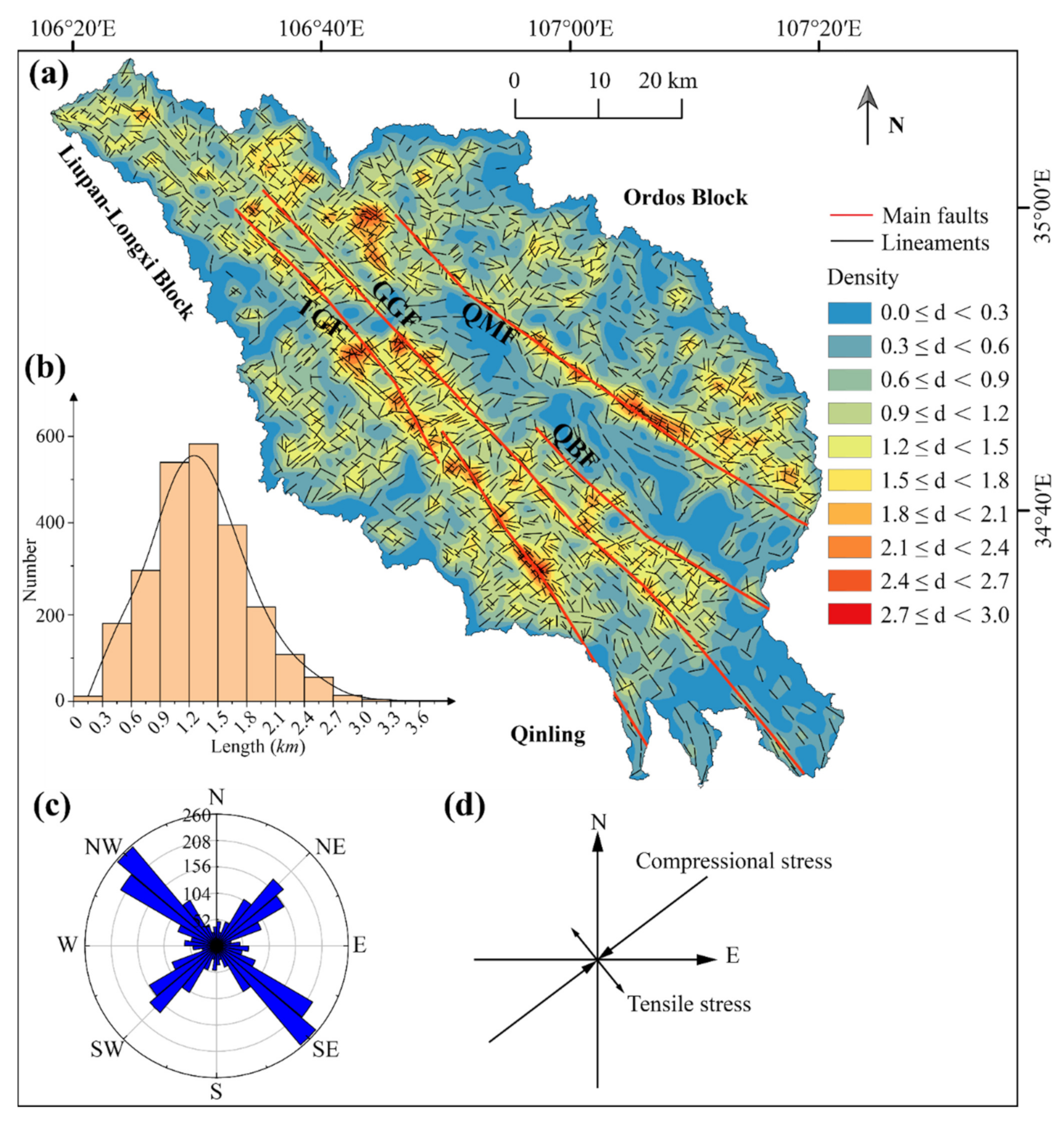
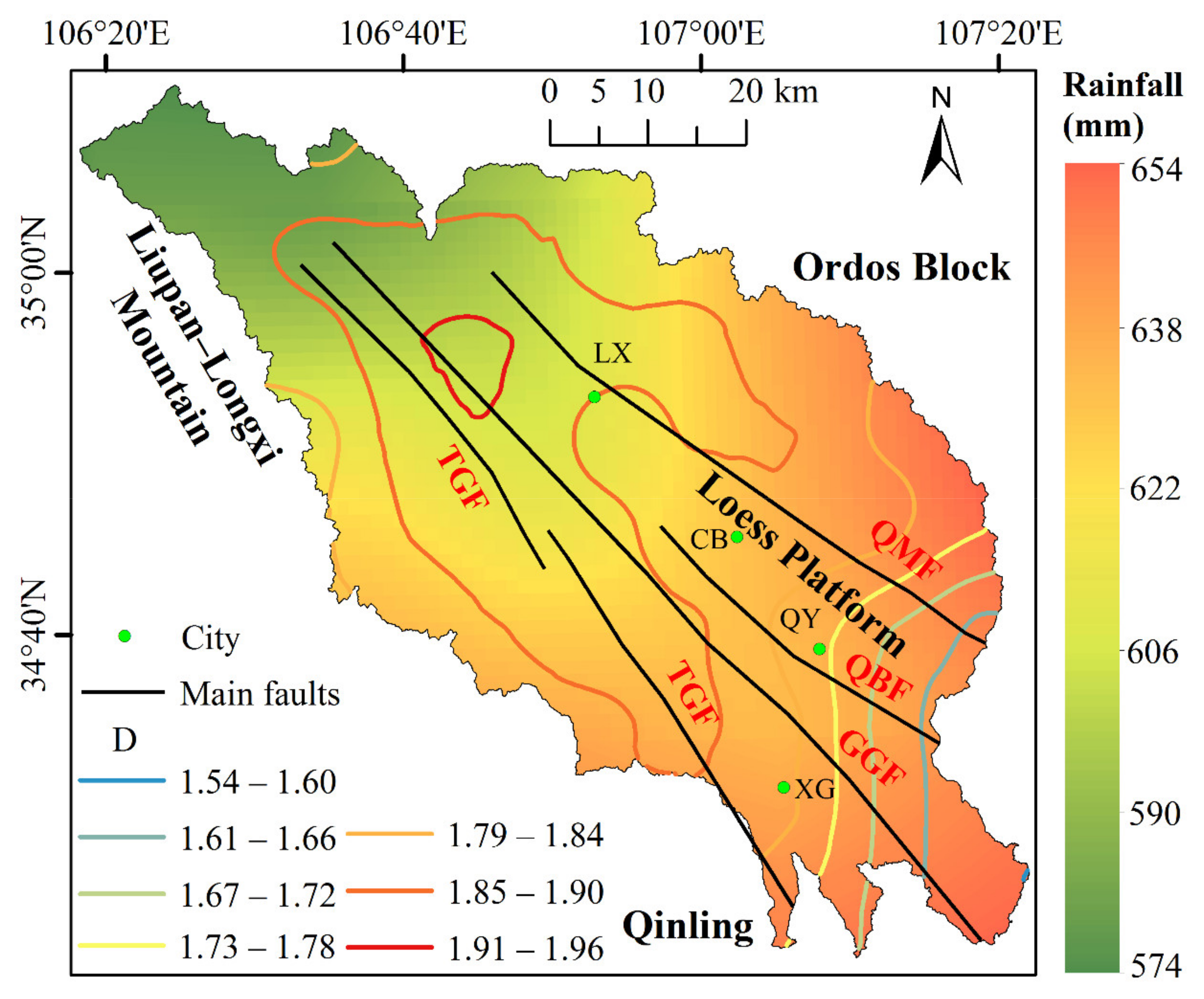
2. Geological Background

The Qianhe River, as the major tributary of the Weihe River, forms part of the shrinking border between the southeastern margin of the Liupan–Longxi Block and the southwestern margin of the Ordos Block [39], located in the middle of the late Paleozoic–Mesozoic basin in the Ordos and the Caledonian orogenic belt in the North Qinling Mountains (Figure 1). The morphology of the area is formed by the four main active faults, with high elevation on both sides but low elevation in the middle. The Taoyuan–Guichuansi Fault (TGF), Guguan–Guozhen Fault (GGF), Qianyang–Biaojiao Fault (QBF), and Qishan–Mazhao Fault (QMF) strike northwest–southeastward (NW–SE) (Figure 1) [44], with an inclination of 50–60°, constituting the boundary between Precambrian and Quaternary. The NW–SE striking faults here mostly follow the course of the Qianhe River in the Qianhe Graben, from northwest to southeast in the study area. Topographically, the TGF, a normal fault, follows the boundary between the southwestern Ordos Block and Loess Platform (Figure 1) [44,45], and it cuts the Loess Platform deeply in the southeast Qianhe Graben, as characterized by straight lineaments in three-dimensional (3D) images [46]. Moreover, previous studies investigated the Quaternary activity of the QMF, displaying left-lateral slip in kinematics with rates ranging from 0.5 to 1.5 mm/year [46]. Other studies have shown that the horizontal and vertical displacements induced by the latest earthquake were about 3.5 and 1.7 m, respectively [47]. During the late Quaternary, the northwest margin of the Qianhe Graben featured a horizontal slip rate of 1–3 mm/year and a vertical slip rate of 0.9 mm/year, while the southeastern margin featured a horizontal slip rate of 2–3 mm/year and a vertical slip rate of 0.2–0.5 mm/year [48] (Figure 1). Although more detailed field work has been conducted here along the strike and fault scarps of QBF [49,50], there is no more evidence to show the Quaternary activity during the late Quaternary, indicating that the QBF is a concealed fault. As for the other normal faults here, TGF and GGF show opposite orientation, with a vertical displacement of 2 m (TGF) and horizontal displacement of 15 m (GGF) [51]. Under the block formation, the horizontal spacing distance of the faults increases gradually from northwest to southeast (approximately 3.9–11.6 m between TGF and GGF, and 8.9–12.1 m between QBF and QMF) (Figure 1), meaning that the density of lineaments will decrease along the faults.

From the lithostratigraphy point of view, more than 50% of the study area is covered by Quaternary loess (Figure 1), and the exposure stratigraphic intervals of bedrock sedimentary strata are from Precambrian to Neogene. Specifically, to the north of QMF, the lithology predominantly consists of Jurassic sand-bearing mudstone to Cretaceous feldspathic lithic quartz sandstone [53], which are mainly exposed to the river valley. Additionally, the exposure stratigraphic intervals of bedrock sedimentary strata are Precambrian quartz sandstone and tuff, Cambrian limestone, Ordovician dolostone, Triassic feldspathic sandstone, and Neogene red clay, which are also present to the north of GGF (Figure 1). Exposed by the eastward extrusion of Longxi Block on the northeastern side of Qinghai–Tibet Plateau [54,55], there are also outcrops such as Cretaceous conglomerate and sandstone between GGF and TGF. By contrast, there is also a wide area of Precambrian red granite and Triassic feldspathic sandstone and siltstone on the west side of TGF (Figure 1). Fieldwork has shown that the bedrock resistance of southern bedrock is larger than that in the northern area [50], suggesting that these areas easily generate more lineaments than the northern margin of the Qianhe Graben.

This region grew rapidly in the Liupan–Longxi Block because of the accelerated extension and structural deformation of the northeastern margin of the Qinghai–Tibet Plateau since the Middle Pleistocene [56]. In the Qianhe Graben, the highest elevation is 2735 m; after flowing through the central loess terrace, the altitude decreases to 548 m. The area with the highest topographic fluctuation is located in the bedrock area on the southern Qianhe Graben and the loess ridge on the northern area, whereas, in the middle part, the loess terrace valley has smaller topographic relief, and the relative altitude between the bedrock area and the terrace valley is over 1000 m. A vast number of valleys, ridges, and other lineaments are created under this context by cutting rivers and rising mountains. On remote sensing images and DEM images, valleys and ridges exhibit apparent linear distribution characteristics [11]. However, the characteristics of faults that can be identified in the research region are few and concealed from the field-measured work [49]. Therefore, the lineaments here have similar orientation; therefore, showing the extraction and fractal characteristics of lineaments tends to be more necessary for tectonic movement and surface processes.

3. Methods

3.1. Lineament Extraction

Previous algorithms related to lineament extraction mainly focused on the extraction of the ridgeline and the valley line, fracture zone, and geological geometry edge in remote sensing images and DEMs (e.g., [19,20,21,22,23,57,58]); therefore, the anomaly gradient pixels can be regarded as lineaments after grayscale transformation. Specifically, on the basis of the filter, edge detection, threshold, etc., the algorithms can be divided into the segment tracing algorithm (STA), LINE algorithm in PCI software, and tensor voting.

3.1.1. Segment Tracing Algorithm (STA)

Taking the STA method as an example, the image was firstly filtered using the median filter to smoothen the image and eliminate much of the noise. Secondly, the pixels were searched in a given search window with an azimuth (θ) and distance (h) at equal intervals to find the continuity of two pixels on the same straight line by obtaining the minimum value of continuity function ε(x) (Equation (1)). Lastly, it was determined whether the pixels were on a line to set the threshold (T) and calculate the pixel change rate (λ) of two points (Equation (2)), before connecting the valley pixels into a lineament [16,59,60]. Previous examples have demonstrated that the improved continuity, stronger reliability, and greater coincidence of measured faults are the benefits of this algorithm [60]. The disadvantage is that the auto-connectivity is not good enough when extracting line segments, which is related to the directional interval and the search window scale.

$$\epsilon (x)={\displaystyle {\int }_{-a}^a\omega (x+h){[z(x)-z(x+h)]}^{2}dh},$$

(1)

$$\lambda =\frac{{\left[\frac{{\partial }^{2}z(x)}{\partial x^2}\right]}^2}{z(x)},$$

(2)

where ω(x) is the weight and a is the distance.

3.1.2. LINE Algorithm in PCI Software

Additional studies mainly focused on edge detection operators (Roberts, Sobel, Prewitt, LOG, and Canny) [61,62], and their identification was mainly based on the operators of derivatives, whereby their optimization can reflect the edge grayscale of lineaments with large variation. Although these algorithms could overcome the problem of interpreter bias, too much noise and false edges still constrained their development [62,63]. In these methods, the Canny algorithm is considered better, providing smoother results; its steps are described below.

(1) Smoothing: The image is filtered with a Gaussian filter to remove the noise as the edge detection is susceptive to high-frequency edges.

(2) Non-maximum suppression: The image gradient is calculated by using the Sobel operator in both x- and y-directions, and then the background pixel and edge pixel are distinguished by checking the gradient magnitude (Equations (3) and (4)), where the magnitude of edge pixels is the local maximum compared with neighboring pixels.

$$g_{xy}(i,j)=\sqrt{g_x{(i,j)}^2+g_x{(i,j)}^2},$$

(3)

$$\theta =\arctan (\frac{g_y(i,j)}{g_x(i,j)}).$$

(4)

(3) Hysteresis threshold: The lineament pixels are obtained after comparing the gradient magnitude of each edge pixel by using the specified hysteresis threshold (g_max and g_min, where g_max is two or three times the value of g_min). More specifically, the pixels whose gradient is larger than g_max are marked as edge pixels, whereas pixels whose gradient is lower than g_min are removed. As for the gradient of pixels within the range (g_min, g_max), the pixels are searched again in the 3 × 3 neighboring pixel domain and kept if the gradient is larger than g_max.

This method offers an algorithm for edge detection according to the requirements for optimization, and it is included in the PCI software [61,64]. However, threshold selection depends on the interpreter, resulting in a small false edge.

3.1.3. Tensor Voting (TV)

According to previous studies [11,65,66], the TV method can be described by the following steps:

(1) Data preprocessing: By using radiometric calibration, atmospheric correction, image clipping, and principal component analysis of Landsat 8 OLI remote sensing images, it is possible to produce and handle the best component as the fundamental data for subsequent analysis. Then, a high-pass Gaussian filter is used to eliminate low-frequency noise [67].

(2) Edge detection: The pixels are encoded into stick-and-ball tensors by tensor voting [68,69]. The attribution of pixels (edge point and non-edge point) relies on combining their significance in the linear combination of the tensor, and the edge pixel points are retained. Each pixel in the remote sensing image forms a tensor with another pixel in the neighborhood; then, a tensor field is formed with all neighborhood pixels. In a different voting scale and path, each pixel receives votes from the neighborhood pixels. Therefore, in all pixels, the final voting outcome is separate. They can be considered as points on the same edge when the salient characteristics are compatible. According to the matrix spectral decomposition, the tensor T can be expressed as a linear combination of eigenvalues and eigenvectors, as follows:

$$T=({\lambda }_1-{\lambda }_2)\stackrel{\rightharpoonup }{e_1}{\stackrel{\rightharpoonup }{e_1}}^T+{\lambda }_2(\stackrel{\rightharpoonup }{e_1}{\stackrel{\rightharpoonup }{e_1}}^T+\stackrel{\rightharpoonup }{e_2}{\stackrel{\rightharpoonup }{e_2}}^T),$$

(5)

where λ₁ and λ₂ are eigenvalues, and λ₁ ≥ λ₂ ≥ 0; $\stackrel{\rightharpoonup }{e_1}$ and $\stackrel{\rightharpoonup }{e_2}$ are the corresponding eigenvectors. $\stackrel{\rightharpoonup }{e_1}{\stackrel{\rightharpoonup }{e_1}}^T$ and $(\stackrel{\rightharpoonup }{e_1}{\stackrel{\rightharpoonup }{e_1}}^T+\stackrel{\rightharpoonup }{e_2}{\stackrel{\rightharpoonup }{e_2}}^T)$ are the stick-and-ball components (Figure 2), whereas (λ₁ − λ₂) and λ₂ are significant indicators of the corresponding stick-and-ball components.

Figure 2 also demonstrates that an ellipse, i.e., the tensor, can be uniquely determined by given values of β, λ₂, and λ₁ − λ₂. The tensor of each pixel is accumulated after voting to get a new tensor T′. The new tensor is decomposed into the form of Equation (5), and the corresponding eigenvalues and eigenvectors are obtained, including the significance index λ^′₁ − λ^′₂ and λ^′₂ of the new stick-and-ball components. The grayscale of lineaments changes rapidly on remote sensing images; consequently, the sum of the vectors of the edge points varies greatly after voting, whereas the sum of non-edge points hardly changes. Therefore, the linear edges can be retained.

(3) Lineament extraction: Even though the lineaments can be shown after tensor voting, their connectivity is still limited. By using Hough transform [71,72], the problem of line extraction in the image space can be transformed into the peak problem in the parameter space, and then the edge point of the image domain can also be transformed into a parameter curve in the Hough domain. Mapping the final lineaments after the cumulative degree of intersection provides the maximum.

3.2. Fractal and Multifractal Analysis

For a long period, the development of faults was not described quantitively, as the surface uplift is not a simple tectonic movement but induced by multiple factors. Therefore, Euclidean geometry cannot accurately describe these series of irregular linear or planar movements. However, the advent of fractal theory has become a new tool to predict or explore this phenomenon, using the dimension as a novel parameter to quantify the geological geometries. A fractal is a shape that remains similar to the whole even after local magnification [73], indicating that no matter how small the object is, it can be well expressed after rescaling, translation, and rotation. These objects are neither totally regular nor random, and the same applies to their so-called self-similarity. The main step is to count the characteristics of geological geometries under various scale conditions and quantify the power-law relationship shown in Equation (6) [25,26,74].

$$N(r)=C{r}^{-D},$$

(6)

where the C is a constant, and the D is the fractal dimension.

3.2.1. Fractal Characteristics

The conventional methods of calculating fractal dimension are the box dimension, circle covering dimension, length–frequency mathematical dimension, and concentration–area dimension [74,75]. In this study, the box dimension method was used to determine the fractal result of lineaments in the Qianhe Graben. Specifically, the grid number N(r) of the square inner body with side length r was calculated, and then the size (r₁, r₂, r₃, …, r_n) of square side length r was continuously changed before calculating the corresponding N(r). If the scattered plot (r_i, N(r_i)) satisfied the power-law relationship shown in Equation (6), the lineaments could be considered to have fractal characteristics.

We obtained the logarithm on both sides as follows:

$$\log N(r)=-D\log r+C.$$

(7)

The limit exists when r → 0, i.e.,

$$D=\underset{r\to 0}{\lim }\frac{\log N(r)}{-\log r}.$$

(8)

Thus, the linear fractal of the region can be determined when the logr and logN(r) show a linear function form, and D is the absolute slope of Equation (7). As a result, the solution of Equation (8) can be transformed into a simple slope absolute problem of Equation (7).

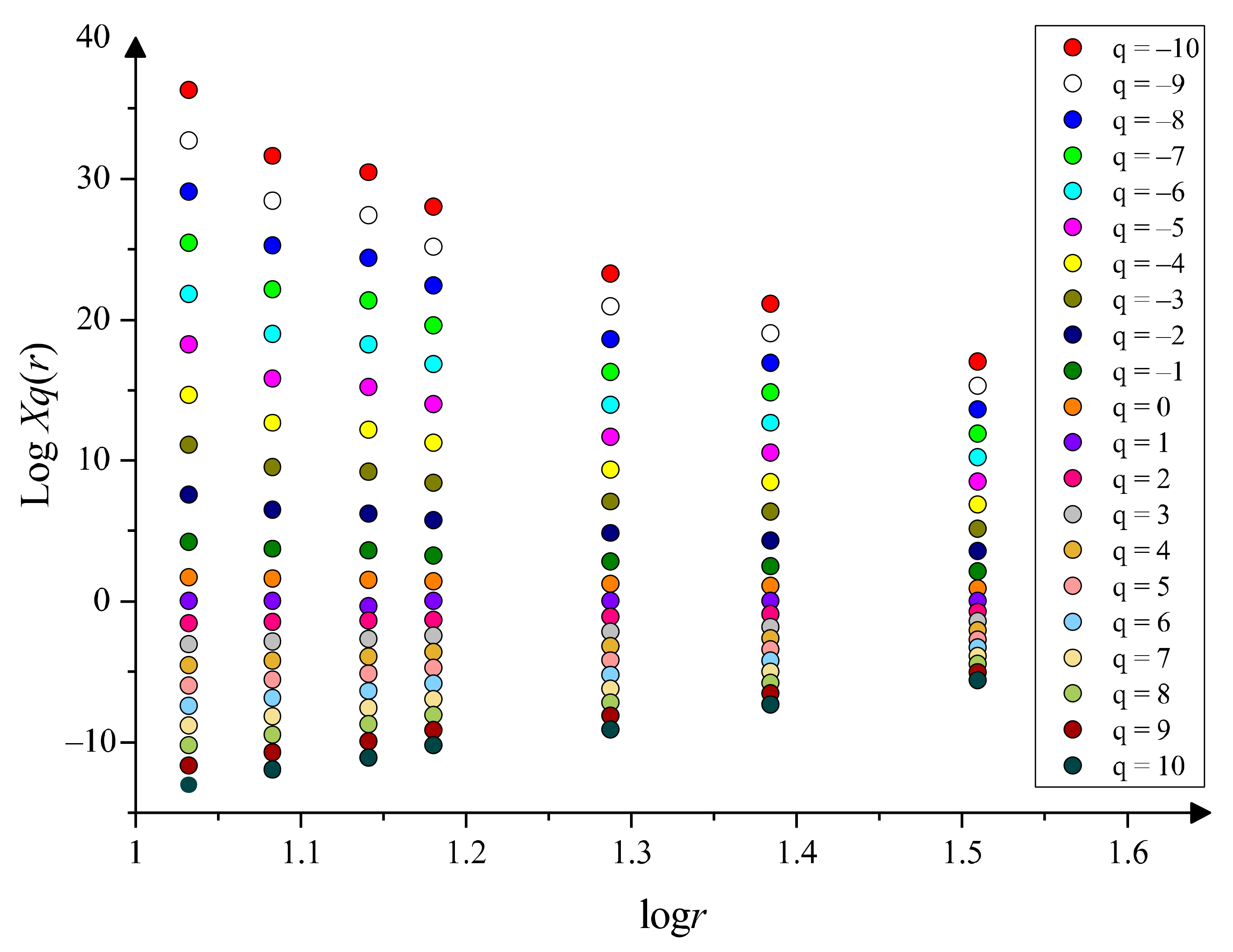
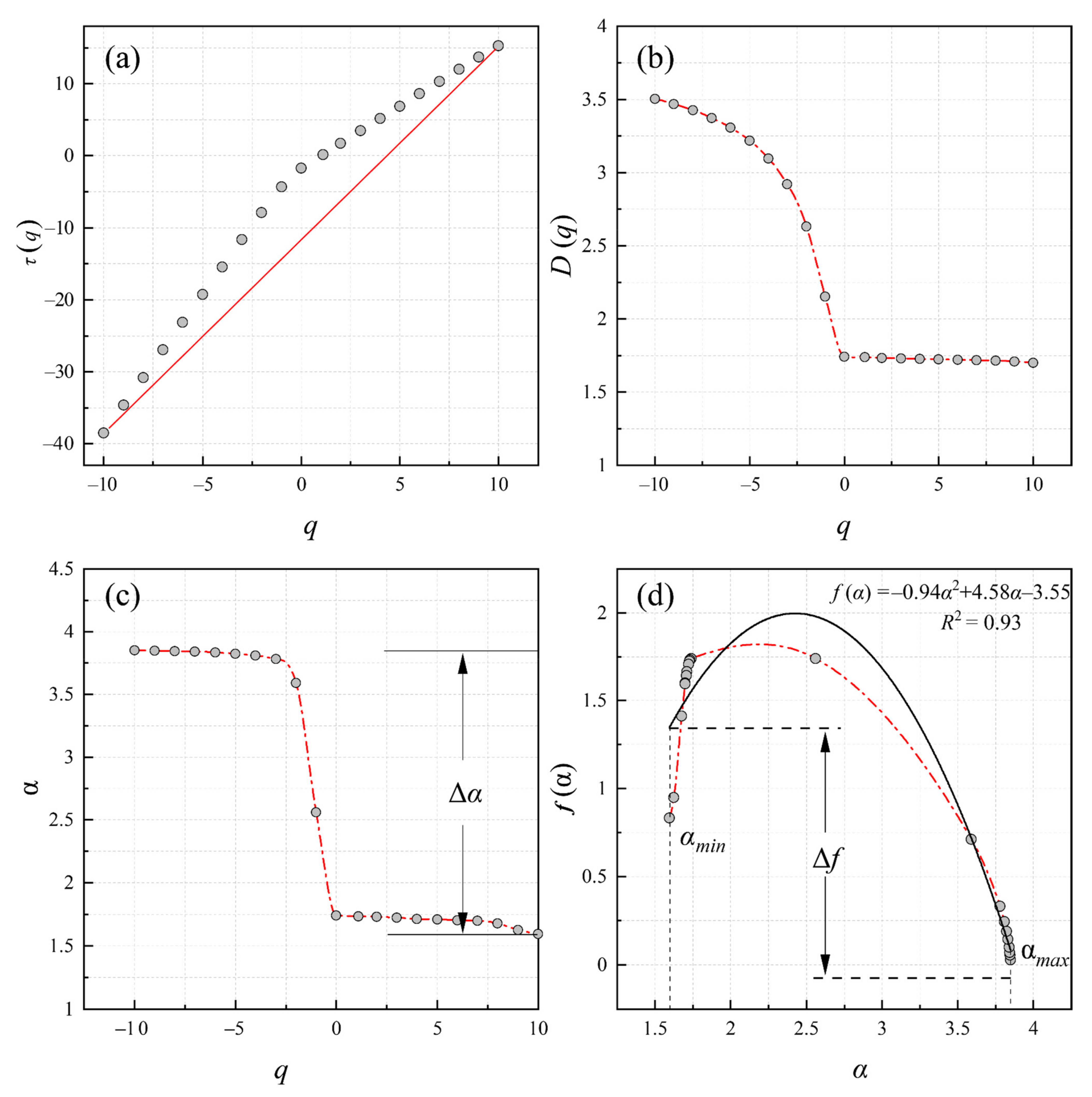
3.2.2. Multifractal Characteristics

Due to the differences among the bedrock uplift, climate change, lithological strength, and mechanical properties, various directions, sizes, and lengths are shown in lineaments in response to the changes in these factors and scales. As the box dimension only considers the number of the boxes and neglects their weight (e.g., the length and density) in the calculation, this complex dynamic geological phenomenon is hard to be characterized and described, as is the dynamic tectonic mechanism of displacement under the faults. In other words, when the objects remain similar to the whole even after local magnification on various scales, it can be said that the objects are multifractals [74,76]. Therefore, a multifractal is a combination of multiple single fractals in space, whereby a single fractal is a special case of a multifractal, and a multifractal is a promotion of a single fractal. In realistic applications, the generalized dimension (D(q)) and the multifractal spectrum (f(α)) can be used to describe the fractal characteristics at various levels [77]. Taking the spatial singularity of branch sets into account, the multifractal method can better reveal the relationship between individual and total in fractal characteristics. It is the normalized probability distribution of the research content in the framework of the research material, which can reflect the complexity and uncertainty of lineaments in various ranges. Specifically, the generalized fractal dimension and multifractal spectrum of lineaments can be calculated as described below.

(1) The study area is covered with small squares of varying sizes (r), and the total length N_i(r) of the inner lineaments of the i-th square is counted. Therefore, the probability P_i(r) that the lineament length in each small square accounts for the total length of the lineaments in the entire region can be obtained as follows:

$$P_i(r)=\frac{N_i(r)}{{\displaystyle \sum _{i=1}^n{N}_i(r)}}.$$

(9)

Different weights of q can be selected (−∞ < q < +∞), and the q order partition function can be defined on the fractal subset as follows:

$${\chi }_q(r)={\displaystyle \sum _{i=1}^n{P}_i^q=r^{\tau (q)}}.$$

(10)

(2) The logarithm of r and χ_q(r) can be obtained, and the result is projected into the coordinate system (logr, logχ_q(r)). The fractal is proven when the slope of the fitting curve τ(q) satisfies the following power-law relationship:

$${\chi }_q(r)\propto r^{\tau (q)},$$

(11)

where τ(q) is also called the mass exponent of q order.

In other words, if τ(q) is a linear function of q, then the lineaments have a single-fractal feature. Conversely, if τ(q) is a convex function of q, it has a multifractal feature [37]. Due to the value of r being different, the lineament complexity will be different.

(3) According to the definition of previous studies [78], the generalized fractal dimension is calculated as follows:

$$D(q)=\frac{1}{q-1}\underset{r\to 0}{\lim }\frac{\ln {\chi }_q(r)}{\ln r}=\frac{\tau (q)}{q-1},$$

(12)

where D(q) is a monotone decreasing function in q. When the q values are equal to 0, 1, and 2, D₀, D₁, and D₂ are the ability dimension, the information dimension, and the correlation dimension, respectively [79]. Specifically, D₀ can characterize the distribution range of lineament length, where a larger value denotes a broader distribution range. D₁ represents the accumulation of lineament length, where a smaller D₁ denotes a more concentrated distribution of lineaments. D₂ describes the uniformity of lineaments at test intervals, where a greater value denotes greater uniformity. In general, the capacity dimension ≥ information dimension ≥ correlation dimension. In particular, when the three dimensions are equal, the distribution of lineaments is a single fractal.

(4) By using the Legendre transformation in physics, the multifractal spectrum f(α)-α can be obtained as follows:

$$\alpha (q)=\frac{d\tau (q)}{dq},$$

(13)

$$f(\alpha )=q\alpha (q)-\tau (q),$$

(14)

where the α(q) is a singular exponent and a monotone decreasing function, which reflects the singularity intensity of lineaments and represents the probability of lineaments in the scope of the study.

Through this treatment, the multifractal can be divided into multiple singularity degrees for further study. Generally, if the α values at different lengths (r) are equal, then the lineaments have a single-fractal characteristic [80]. On the contrary, when the singular exponent is a monotone decreasing function in q and the α values are different [81], then it has multifractal characteristics. Within the fault zone, the spectral width Δα = α_max − α_min is used to describe the uniform state of the probability distribution, such as the length and density of the fracture, where a larger Δα denotes a more violent fluctuation of lineament length, resulting in a more uneven probability distribution. Unlike D(q) and α(q), the fractal spectrum (f(α)) is a convex function of an approximate parabola [81], and its symmetry is generally expressed as shown in Equation (15). Previous studies have shown that a grid number with large probability is larger than a grid number with small probability when f(α) is a left-hook curve [3]. By contrast, a grid with a small probability has a higher number when f(α) is a right-hook curve [82]. This feature can refer to the range of development and stability of regional faults.

$$\mathrm{\Delta }f=f({\alpha }_{\min })-f({\alpha }_{\max }).$$

(15)

4. Results

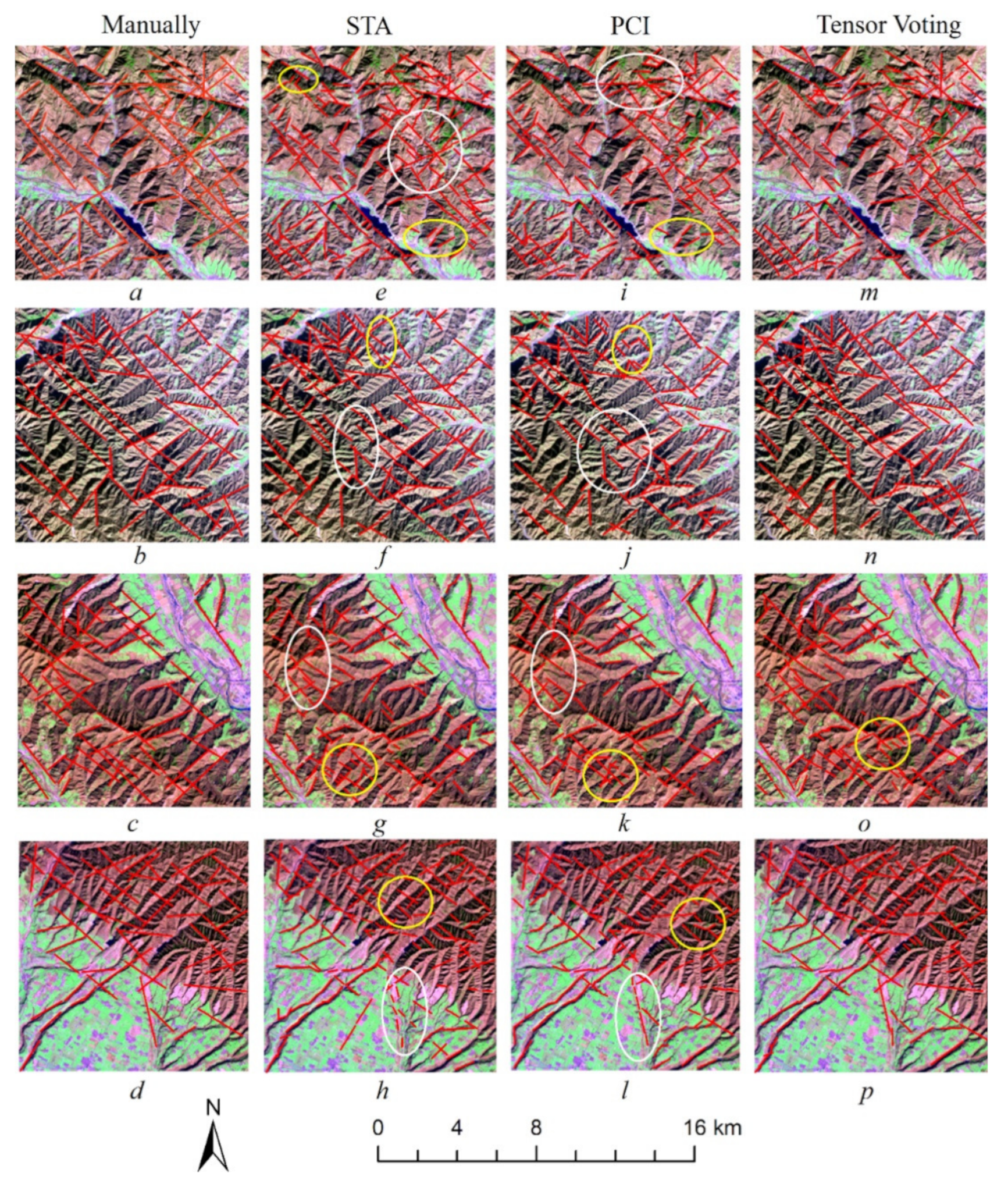
4.1. Lineament Extraction and Validation

4.1.1. Lineament Extraction Results

Considering the number of remote sensing images and the processing ability of the computer, the subareas (a), (b), (c), and (d) in Figure 1 were used as the basic data for subsequent processing. Firstly, to verify the accuracy, the lineaments obtained by visual interpretation of the four subareas were used as known lineaments and verified by 30 researchers in geology, geomorphology, and remote sensing (Figure 3a–d). Furthermore, the STA, PCI, and tensor voting algorithms were used to extract the lineaments of the study area (Figure 3e–p).

On the basis of the visual result, the three algorithms could identify the lineaments of the study area to a great extent, but the extraction effect was different. The regional lineaments in the study area were mostly near the ridgeline and valley line (Figure 3a,b), the geomorphological dividing line (e.g., the dividing line between the mountain and plain) (Figure 3c,d), and the fault/fracture zone, which is highly consistent with previous theoretical findings [11]. The lineaments extracted by the STA and PCI algorithms were shorter than the known interpretation results, especially in the mountainous area (a) and (b) in Figure 3, where the terrain is more complex and the gully ridge is crossed. Therefore, there was a lot of noise (yellow elliptical field in Figure 3) full of false edges, while the tensor voting algorithm generated little or no noise. The presence of noise is linked to the fragmentation of the landscape in the covered area. For instance, in the areas with dense lineaments (Figure 3a,b), the exposure stratigraphic intervals of bedrock sedimentary strata were mainly Ordovician dolostone, Triassic feldspathic sandstone, and Cretaceous conglomerate, indicating that these areas are not stable and easily generate more lineaments. Consequently, the degree of fragmentation was greater than the edge pixels of lineaments. There were also some over-detection phenomena in the terrace area, whereas linear pixels, such as roads, were also identified as lineaments (Figure 3h), as related to the edge detection algorithm (where the results from STA are related to the line pixel direction change rate threshold T, while PCI uses Canny edge detection). However, these roads detected as the lineaments are false edges and should be removed. Moreover, the continuity of lineament segments generated from STA and PCI algorithms was also worse than that from tensor voting (the white elliptical region in Figure 3). More specifically, in a similar direction, the lineaments generated from these algorithms did not link into a line as the interval was too large. Therefore, increasing the search radius to complete the link seems more necessary. Furthermore, redundant or repeated edges often appeared in the results, which led to increasing noise and a higher false detection rate, and some lineaments were even inconsistent with the real geomorphological phenomena. The advantage of tensor voting is that it relies not only on the surrounding pixels but also on other data sources, such as DEMs. Furthermore, there was a binary noise reduction after the high-pass Gaussian filter. Additionally, with the tensor voting algorithm, the missing detection rate was low since only small noise edges were observed, and the position in the dense voting was more reliable, making the algorithm more stable. Visually, the lineaments derived by tensor voting were more consistent with the known lineament results, followed by the STA and PCI algorithms.

4.1.2. Accuracy of Lineament Algorithm

To ensure the accuracy of the initial fractal dimension, the premise is to achieve higher-precision lineaments. The total number was firstly calculated, as shown in

Table 1. The total number of lineaments in the four subareas of the Qianhe Graben. STA, segment tracing algorithm.

Region	Manually	STA	PCI	Tensor Voting
(a)	65	213	183	185
(b)	58	146	123	114
(c)	55	205	128	147
(d)	55	206	238	140

. The total number of the lineaments extracted from STA was the largest while the manual method produced the smallest. The tensor voting algorithm produced a larger total number than the PCI, and this difference occurred in the subareas (b) and (d).

Additionally, due to the existence of false edges of lineaments, more quantitative analyses are needed to evaluate the accuracy of these algorithms. In all sections detected as lineaments, non-lineaments may be included, but they are all regarded as lineaments. The accuracy is good only when the segments are detected close to the reference map. Therefore, four indices (accuracy (A), precision (P), recall (R), and F1) were used, described in Equations (16)–(19) [66]. The statistical results are shown in

Table 2. Comparison of accuracy using different algorithms. TV, tensor voting; TP, true positive; FP, false positive; FN, false negative.

Region	Methods	TP (km)	FP (km)	FN (km)	A (%)	P (%)	R (%)	F1
(a)	STA	125.19	41.24	39.07	68.47	75.22	76.21	0.76
	PCI	114.32	45.02	49.69	62.06	71.75	69.70	0.71
	TV	146.19	29.59	21.43	81.45	83.17	87.22	0.85
(b)	STA	130.19	32.40	25.32	78.52	80.07	83.72	0.82
	PCI	111.67	30.21	38.64	68.56	78.71	74.29	0.76
	TV	131.50	28.90	23.72	80.03	81.98	84.72	0.83
(c)	STA	98.61	29.68	23.45	74.35	76.86	80.79	0.79
	PCI	102.27	22.68	19.24	78.87	81.85	84.17	0.83
	TV	109.34	24.49	13.34	83.56	81.70	89.13	0.85
(d)	STA	90.69	27.09	20.97	72.11	77.00	81.22	0.79
	PCI	94.33	28.69	17.74	74.52	76.68	84.17	0.80
	TV	107.12	20.11	7.59	86.31	84.19	93.38	0.89

.

$$A=\frac{\frac{TP}{TP+FP+FN}+\frac{TP}{D}}{2}\times 100,$$

(16)

$$P=\frac{TP}{TP+FP},$$

(17)

$$R=\frac{TP}{TP+FN},$$

(18)

$$F1=\frac{2P\times R}{P+R},$$

(19)

where D represents the total length of the lineaments known to be interpreted, TP represents the length of true lineaments detected as lineaments, FP represents the length of non-lineaments detected as lineaments, FN represents the length of true lineaments detected as non-lineaments, A defines the ratio of the correct part of the linear results to all the results detected, P describes the ratio of the correct detections to all parts detected as lineaments, and R represents the ratio of correct detections to all lineaments, where all lineaments include not only the true lineaments detected correctly, but also the true lineaments ignored. The F1 value is the harmonic index of P and R, and its value ranges from 0 to 1. A larger F1 denotes a better ultimate result.

Specifically, in region (a), the A value derived by the LINE algorithm in the PCI software was the lowest (62.06%), which represents that the proportion of correct lineaments was lowest in the region with all detection results. The main explanation is that the algorithm extracted the least correct results in the region (114.32 km). By contrast, the FP value was the largest (45.02 km), which means that many edges that were non-lineaments were recognized; thus, the P value was lower. The FN value was also the largest among the three algorithms, suggesting that the edges of the lineaments were not effectively identified, resulting in the lowest recall rate R. Upon synthesizing the P and R results, the region was found to have the lowest F1 value (0.71). Subregion (a) is located at the northern part of the Qianhe Graben and is jointly controlled by the three faults TGF, GGF, and QMF (Figure 1). The spacing between the faults is 3.5 km (TGF–GGF) and 9.6 km (GGF–QMF). The surface height is continuously uplifted and the river is eroded by the water system in the areas of dense fault distribution. As a result, more nonlinear edges (such as roads and mountain shadow lines) were also identified as lineaments, while the local linear uplift of the surface caused by faults was not detected. Therefore, the lineament extraction effect of the PCI algorithm in the area with a complex surface coverage was worse.

Similar to region (a), region (b) was located in a hilly area with serious surface breakage, with the difference being that the area is only controlled by the two faults of TGF and GGF, where the distance between the faults is 3.9–4.5 km. As a result, this region has less surface fragmentation, and fewer lineaments were detected than in region (a), but they were longer in length. The TP and FN values in the extraction results of the STA algorithm were close; thus, the A and R values of the two algorithms were closer, meaning that the extraction results of STA and TV were more consistent in the complex terrain fragmentation. However, the TV algorithm was slower than STA, and PCI was fastest, which was related to the method of edge detection. Hence, when extracting such lineaments, the TV algorithm can be substituted with STA.

The difference between region (c–d) and region (a–b) lies in the terrace plain areas, which led to the TP values of lineaments in region (c) extracted by STA being lower than those extracted by the PCI and TV algorithms, with the latter two methods are closer. Therefore, the correct proportion of lineaments extracted in the plain region was lower. Notably, the FP extracted by PCI was lower (22.68, lower than 24.49 obtained using the TV algorithm); that is, few edge pixels which are non-lineaments were recognized as lineaments in this region. Nevertheless, the FN value of this algorithm was lower, and some lineaments were not effectively recognized using the LINE algorithm in PCI. As a result, the F1 value of the two algorithms was only 0.02, whereas the extraction result from the TV algorithm was optimal.

As for area (d), divided by the QMF, the loess occupies the terrace to the south of the fault, and the ridge is to the north of the fault. The results were inferior to those of the PCI and TV algorithms in region (c) derived by the STA algorithm. In this field, the coverage of the terrace area is larger, resulting in discontinuity of the linear edge in the valley area, and then the FN value in the PCI algorithm was larger than that in the TV algorithm. Meanwhile, the areas with some noise, such as roads, which are non-lineaments, were also identified as lineaments, resulting in higher FP values for PCI and STA. The difference in F1 values between PCI and STA in the region was only 0.01; therefore, it was not of much practical significance to simply study the P and R values in this subarea. For geologists, it is more desirable to extract results with larger F1 values, such as the F1 obtained using the TV method.

Therefore, in terms of accuracy, the TV algorithm is more reliable in areas with higher surface fragmentation, followed by STA and PCI, whereas the LINE algorithm in PCI is better than STA in areas with complex forms of geomorphology. All of these findings show that the TV algorithm has a better detection effect and greater coincidence with results of visual interpretation. These findings can be utilized in the study of lineament extraction and further analysis of the fractal dimension. To further analyze the lineament characteristics of the Qianhe Graben, a lineament distribution map of the entire area was extracted using the TV algorithm (Figure 4).

Firstly, the lineament density in this area ranged from 0.0 to 3.0 fractures per km², and a higher density was distributed near the four active faults (Figure 4a). The distribution also showed the main location and distribution direction of the faults in the Qianhe Graben. In other words, the lineament extraction results can serve as the interpretation marker of regional faults. These lineaments are the linear segments and structures caused by different stresses with similar directions in this area. In addition, the uplift of the fault causes the surface to be squeezed and broken, and more lineaments are denser closer to the fault. The density of the southern lineaments was larger than that of the northern lineaments (the average density in the southern area was 0.23, while that in the northern area was 0.19) (Figure 4a). At the same time, the spacing of faults gradually affected the density of lineaments, i.e., a smaller spacing led to greater density and vice versa. The density of lineaments in the entire area decreased gradually from northwest to southeast, which was related to the gradual decrease in spacing between faults. In brief, the tectonic uplift of the southern area in the Qianhe Graben is greater and decreases gradually from northwest to southeast [39].

Secondly, a total of 2454 lineaments were extracted from the Qianhe Graben in the total area with an average length of 1316.3 m, which was related to the range of loess coverage. The average length in the southern region was larger (1354.9 m) than that in the northern region (1274.1 m). The length and number of lineaments approximately followed a normal distribution, among which 596 lineaments with a length of 1.2–1.5 km reached the maximum (Figure 4b). Due to the coverage of loess, a large number of lineaments were unexposed. The length of lineaments that could be identified was, thus, shorter. A higher hilly area is more likely to generate and more easily generates lineaments relative to the loess terrace in the middle. In other words, areas that can be identified as lineaments have greater potential to form faults.

Lastly, the lineaments of the region had a main direction of NW–SE, followed by NE–SW (Figure 4c). Previous studies used high-precision GPS observations from the China Crustal Movement Observation Network to build a plate kinematic model of crustal deformation in the Fenwei Basin, China [83,84]. The results also showed that the current tectonic strain feature of the Qianhe Grabren is the interior of the NE–SW compressional stress, whereas the shallow part is subject to NW–SE tensile stress (Figure 4d). Therefore, the number of lineaments in the NW–SE direction is greater than that in the NE–SW direction. In particular, the Ganqing Block in the western margin of the Qianhe Graben shows compressional strain with an approximately NE–SW direction. All of these results are consistent with the first and second directions of lineaments in the Qianhe Graben. We note that tectonic strain is a complex process, and we cannot use these lineament directions to directly replace tectonic strain in the Qianhe Graben; however, this measure provides new insights to estimate the direction of tectonic strain.

In summary, through the analysis of the length, density, and direction of lineaments, the location, range, and direction of fault events in this area were estimated, which has great geological significance for exploring the tectonic history of this area.

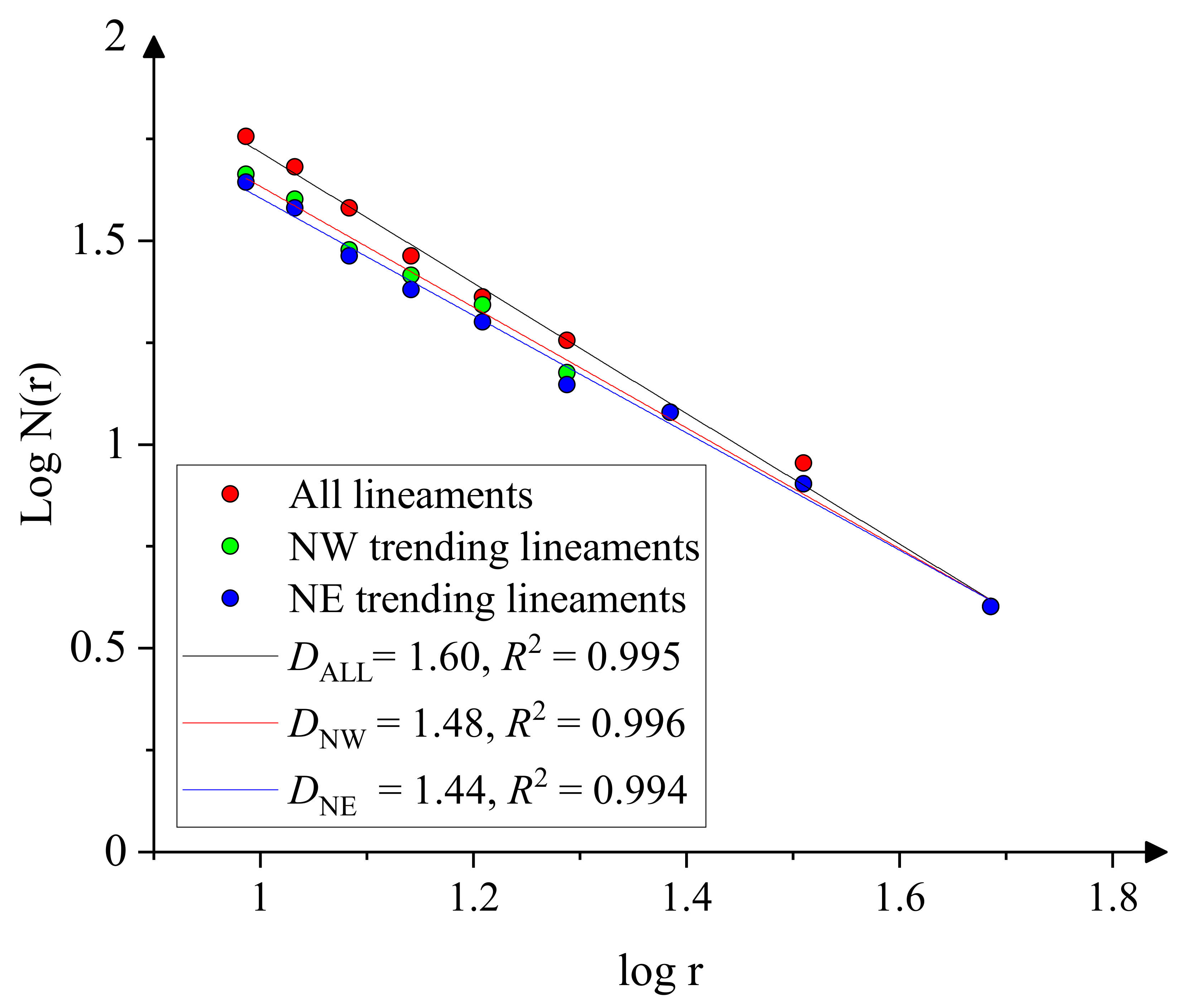
4.2. Fractal Characteristics

In the Qianhe Graben, the fractal dimensions of lineaments in the region were primarily calculated using the steps below.

(1) The Qianhe Graben was taken as the reference, and a square with a length of L = 97 km was drawn to cover all lineaments in the entire area.

(2) The side length of the square was changed, i.e., r = L/2, L/3, L/4, L/5, L/6, …, as well as the covering on the lineaments. As a result, there were 2², 3², 4², 5², 6², … small squares covered, and the number of small squares containing lineaments was calculated as N(r).

(3) According to Equation (7), the logr–logN(r) curve was drawn and fitted using the least square method, where D is the absolute slope of the straight fitted line. The correlation coefficient (R²) was used to assess whether the lineaments have fractal characteristics, that is, whether they have statistical self-similarity or not.

As shown in Figure 5, the box dimension in the 97 × 97 km² grid cells of the lineaments across the whole Qianhe Graben was 1.60, and the box sizes for this box dimension were 48.5, 32.2, 24.3, 19.4, and 16.2 km. There was an excellent linear correlation between logr and logN(r), with a higher coefficient (R² = 0.995). Therefore, the lineaments in the study area showed statistical self-similarity and fractal characteristics. Since the main directions of lineaments in this area were NW–SE and NE–SW (Figure 4c), to further study the fractal characteristics of lineaments in different directions in Qianhe Graben, their fractal dimensions were also determined in these directions. According to fractal theory and Equation (7), D_NW and D_NE were estimated, with values of 1.48 and 1.44 (R² > 0.9), respectively (Figure 5). Therefore, the lineaments in different directions also showed fractal characteristics and good self-similarity. As the fractal value in the NW–SE direction was greater than that in the NE–SE direction, the faults in the former direction were more active and well developed.

To further analyze the spatial distribution of the fractal characteristics of lineaments in the Qianhe Graben, the study area was divided into squares with a length of 9.7 km, where the box sizes for measuring the box dimension in each 9.7 km² cell were 4.8, 3.2, 2.4, 1.9, and 1.6 km. By caring out kriging interpolation, a fractal dimension isogram was drawn and superimposed with the faults in the study area (Figure 6). The overall fractal dimension of the Qianhe Graben lineaments was higher with a mean value of 1.80 (1.53–1.98), slightly higher than the box dimension of 1.60 in Figure 5, which was related to the spatial distribution of lineaments in the Qianhe Graben.

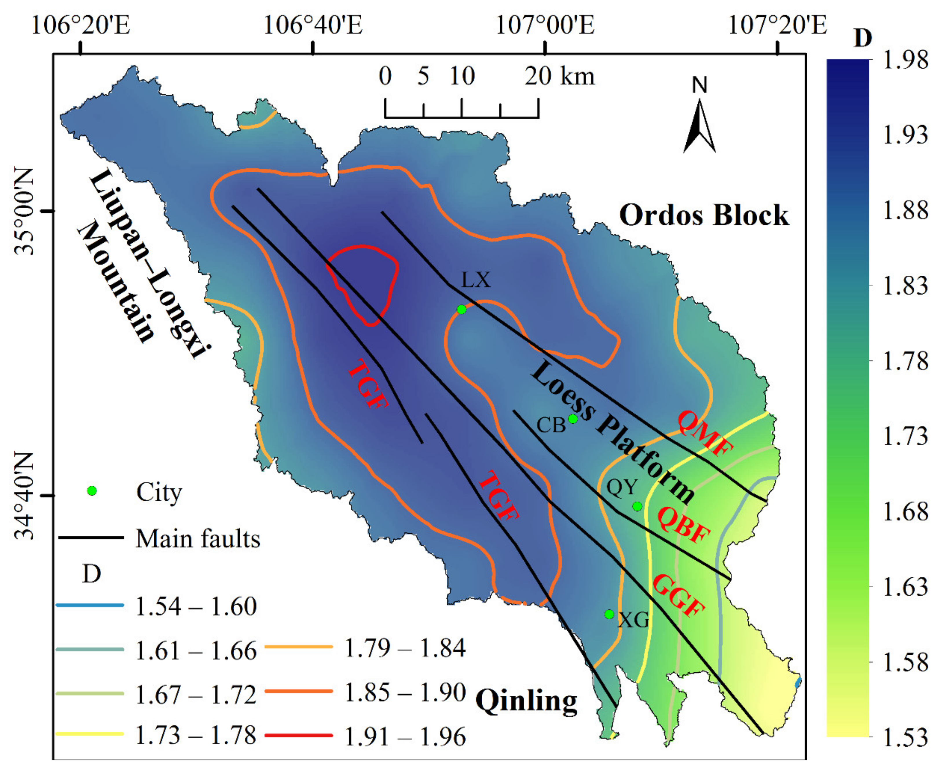
4.3. Multifractal Characteristics

In the Qianhe Graben, small squares with various side lengths r = L/3, L/4, L/5, L/6, L/7, L/8, and L/9 were used to cover all the lineaments. After determining the length and probability of the lineaments in the squares using Equation (9), a logXq(r)–logr diagram was drawn under different q values by transforming different weights of q (Figure 7). The weights of q ranged from −10 to 10 with a step size of 1. As shown in Figure 7, with an increase in q, logXq(r) maintained a good linear attenuation and aggregated to logXq(r) = 1. Therefore, the power-law relationship with logr in Equation (11) was fulfilled by logXq(r). In the specified scale range, the graph had higher scale invariance, showing the tendency of the partition function of probability changing with the side length under different weight factors q, and the multifractal characteristics appeared to be more evident. When q > 0 and q < 0, logXq(r)–logr showed linear characteristics with a slope (≠0), whereas, when q > 0, logXq(r) changed more rapidly (Figure 7). By contrast, logXq(r) varied more slowly when q < 0. When q was close to 1, logXq(r) was closer to the transverse axis. As the weight factor decreased, smaller local features were effectively highlighted. In other words, the focus of the large scale was the fractal feature of lineaments as a complex element in the entire region, which is a global self-similar feature, whereas the small scale highlighted the local fractal features.

As shown in Figure 8a, the slope τ(q) of the fitting line between logXq(r) and logr was obtained. Even though τ(q) increased with q, there was not a linear relationship between them. Specifically, when q < 0, τ(q) grew almost linearly; however, when q = 0, the growth rate of τ(q) slowed down and gradually deviated from the original linear relationship (the red line in Figure 8a), resulting in a broken line shape. Therefore, τ(q) was not a linear function of q, indicating that the lineaments in the Qianhe Graben have multifractal characteristics.

As shown in Figure 8b, the generalized fractal dimension D(q) was a monotone decreasing function, in line with the characteristics of the multifractal dimension. The values of D₀, D₁, and D₂ were 1.744, 1.737, and 1.728, respectively, i.e., D₀ > D₁ > D₂, indicating that the lineaments in the Qianhe Graben are not single fractals. D₀ = 1.744 shows that the lineament length was widely distributed, being closer to the fractal dimension of fault structures in Weibei Plateau (1.45), Weihe Basin (1.55), and North China (2.01), which indicates that the fault activity in this area is complex and coincides with the background of block movement and contact zone. D₁ did not tend to 0, indicating that the lineaments are scattered in some regions, whereas D₂ indicated that lineaments are more uniform in the test interval.

Similar to D(q), α(q) was also a monotone decreasing function (Figure 8c), in line with the characteristics of multifractals. Here, α(q) depicts the change speed of mass index τ(q). Thus, the range of α(q) determines the domain and symmetry of fractal spectrum f(α). The value of α(−1) is located in the middle of the curve, and the spacing with α(0) is shorter than that with α(−2). Therefore, it can be inferred that f(α) is the left deviation. The multifractal width (Δα) in this area was 2.25, which is larger than that of previous studies, as shown in

Table 3. Multifractal width with different areas.

No.	Region	Δα	References
1	Fault zone of Jiaozuo mining area in Henan, China	0.3–2.0	[82]
2	Altay, Xinjiang, China	0.81	[36]
3	Tongling metallogenic area, China	1.35	[74]
4	Northeastern Yunnan Pb–Zn metallogenic belt, China	1.60	[3]

.

The multifractal spectrum f(α) appears as a parabola, which is typically a left-hook shape (the red line in Figure 8d). To better describe its distribution, the quadratic equation fitting (f(α) = A(α − α₀)2 + B(α − α₀) + C) can be adjusted and calculated [86], where the parameter B describes the symmetry of the fractal spectrum. When B = 0, then f(α) is symmetric, whereas, when B ≠ 0, f(α) is a left deviation or right deviation. Here, f(α) was still a left hook, as shown by the black line in Figure 8d, and it reached the maximum at α = 2.44. According to Equation (16), Δf was calculated with a value of 1.21 (>0). Therefore, f(α) was not symmetrical and the length of regional lineaments was different.

To sum up, the mass index, generalized fractal dimension, fractal width, and fractal spectrum of lineaments in the Qianhe Graben all show that the length of lineaments in this area is in accordance with multifractal characteristics. Moreover, by expanding the range of q, even if the positive and negative values tended to be infinite, the changing trend of each graph in Figure 8 could not be altered [87], and the influence on τ(q), D(q), α(q), and f(α) was minimal.

5. Discussion

5.1. Why Do the Lineaments Have Fractal and Multifractal Characteristics?

Previous studies mainly focused on lineament extraction and fractal analysis, ignoring the causes of fractal characteristics. The cause of fractal characteristics depends on the formation and development of tectonic processes. Thus, what is the main cause of the fractal characteristics seen in lineaments in the Qianhe Graben?

Firstly, all lithological strata are covered by the lineaments (Figure 1 and Figure 4) and only differ in the density of lineaments. Thus, the lineaments are not mainly controlled by the lithological formation. Secondly, as the rainfall also has an impact on the surface fragmentation, more valley lines are identified as lineaments. Therefore, annual mean rainfall data were derived from the Tropical Rainfall Measuring Mission (TRMM TMPA/3B43, https://trmm.gsfc.nasa.gov/ (accessed on 29 December 2020)) over the past 20 years, with a range of 574–654 mm (Figure 9); however, they did not show the same pattern with the fractal dimension isogram. Therefore, the climate is not the main reason for the lineaments. Lastly, previous studies have shown that the lineaments can be generated in a fault zone, and they have a higher fractal dimension [3,5]. Other studies have also addressed that the distribution of lineaments is related to the seismic activity and can be transformed into faults. Specifically, the surface fragmentation was attributable to the northeastward extrusion induced by the May 2008 Wenchuan earthquake [83], gradually permeating to the Liupan–Longxi Block. As a result, more lineaments in the NW–SE direction concentrated in the Qianhe Graben and linked into big faults. Furthermore, the lineaments can reflect the bedrock deformation and stress concentration caused by the faults and seismic activity. Similar to these studies, the lineaments in the Qianhe Graben were near to the four active faults (Figure 4a), which could be verified from fieldwork [49,50]. Therefore, the lineaments were most likely generated from the changes in tectonic processes and seismic activity.

In addition, as shown in Figure 4b, the main direction of lineaments in the Qianhe Graben is NW–SE, similar to the main active faults. Moreover, the lineaments around faults have a higher density (Figure 4a). As in the western parts of Weihe Basin, previous studies have shown that the regional stress–strain field of the Qianhe Graben mainly underwent three evolutionary stages: early Tertiary, Miocene, and Pliocene–Quaternary [83,84,88]. The principal stress field changed from tensile stress in the NWW–SEE direction in the early Tertiary period into the extensional stress from NW–SE to NE–SW direction in the Miocene period. However, due to the crustal material of the Tibetan Plateau tending to move eastward [83,89], the compression regime is formed by the collision of the eastward-moving crust with the Ordos block. Therefore, during the Pliocene–Quaternary period, the compressive strain in the NE–SW direction dominated in the Qianhe Graben, followed by the tensile stress in the NW–SE direction. Furthermore, the direction of lineaments is also consistent with the tectonic strain field, indicating that the lineaments could be used as an aid to analyze regional tectonic stress fields, whereby the lineaments were mainly generated from the changes in regional tectonic strain. All of these results suggest that the lineaments in the Qianhe Graben have a self-similarity, and the shapes of τ(q), D(q), α(q), and f(α) showed that the lineaments have multifractal characteristics.

5.2. Analysis of the Fractal Dimension and Multifractal Characteristics in the Qianhe Graben

To compare with other regions, the box fractal dimensions in different regions were determined, including ore bodies and fault zones, with the statistical results shown in

Table 4. Box dimensions of different regions.

No.	Region	Box Dimensions	References
1	Polymetallic ore field in Hutouya, China	1.09	[4]
2	Jiuyi Mountain fault zone in southern Hunan, China	1.12	[90]
3	Maoping Pb–Zn Mine in Zhaotong, Yunnan, China	1.28	[91]
4	Metallogenic area in Tongling, China	1.29	[74]
5	Shanghang–Yunxiao metallogenic belt, China	1.36	[92]
6	Central Sichuan Basin fault zone, China	1.53	[93]
7	Pb–Zn district in Fozichong, China	1.53	[75]
8	Croatia Zumberak Mountain fault zone, Croatia	1.69–1.78	[94]
9	Pb–Zn metallogenic belt in Northeastern Yunnan, China	1.98	[3]

. The results suggest that the box dimension of lineaments in the Qianhe Graben is in the middle and upper deviation. In the Qianhe Graben, the area where the fractal dimension value is greater than 1.8 was mainly concentrated in the mountains on the northwestern and hilly areas on both sides of the Qianhe River. In these regions, more lineaments were generated by tectonic uplift, and the fault spacing was smaller than that in the southeastern; thus, more lineaments were identified, and the fractal dimension was higher. The area with the highest fractal dimension was located at the outlet of the tributary at the northwestern end of Longxian County (LX) (Figure 8). In this area, the distance between faults reached the minimum (3.5 m) [50]; thus, the tectonic activity was stronger and the fractal dimension was higher. In addition, the fractal dimension decreased gradually from northwest to southeast, which indirectly reflects a similar trend of tectonic activity in this area. By contrast, the fractal dimension in the loess terraces, such as Longxian–Caobi, was less than 1.8, which indicates that the tectonic activity of the terrace around the main stream was lower than that of the mountain range on both sides.

Specifically, the width of fractal spectrum Δα in the Qianhe Graben was larger than 0, showing that the lineaments in the study area have multifractal characteristics; furthermore, the range of length change is large and the range of length is wider, denoting that the sizes of lineaments in Qianhe Graben are variable. However, the asymmetry (Δf) was also greater than 0, which indicates that the lineaments with longer lengths were more common than shorter lineaments; that is, the scale of lineaments in this area is mostly large–medium range. Previous studies have shown that, when the multiple fractal spectrum is a left-hook curve, there are more faults of medium and small scale in the region [3,5]. On the contrary, when the multiple fractal spectrum is a right-hook curve, there are a few large faults in the region [82]. The multifractal spectrum of lineaments in the study area was a left-hook curve (Figure 8d). Thus, the lineaments are medium–small scale. The reason for this difference is that the lineaments are discontinuous in space, and the faults connect better. Therefore, the multifractal spectrum is mostly a left-hook curve.

In addition, previous studies have shown that the fractal dimension of the fault is 1.22–1.38 [36], and the difference is mainly related to the change in fault direction and basement lithology. According to this study, when the regional fractal dimension D is larger than that of the interval, the faults in this region are more continuous in direction and the lithology permeability of the basement is stronger. In the formation of fault processes, the fault acts continuously on the distribution and formation of geomorphology and lithology, before gradually stabilizing in the region. Therefore, the fractal dimension of fault events is variable, which leads to the multifractal distribution of regional faults. Moreover, the generalized fractal dimension D of lineaments in the Qianhe Graben was 1.744, which is larger than the interval (1.22–1.38), indicating that the fault distribution in the Qianhe Graben is more complex and still active, controlling the formation and distribution of regional morphology, lithology, mineral resources, and groundwater.

Lastly, previous results have also shown that the D value is related to the complexity of the regional fault [95]; that is, a larger D value denotes more complex regional fault activity and less stable regional faults. When D$\in$ (1.5, 1.8), secondary faults are few but still visible and complex. Although tectonic activity is strong, it is not frequent [95]. Over time, original smaller faults gradually mature, connecting to form a larger fault. The D values of lineaments in this graben belong to the interval (1.5, 1.8), which is sufficient to prove that the graben has small but unstable fault development, with complex and strong activity, which is still not frequent. This is why more fault features cannot be found in field exploration, while interpretation features can be found on remote sensing images.

In summary, the multifractal characteristics of lineaments in the Qianhe Graben show that the faults in this area are of medium scale and easily generate tectonic lineaments.

6. Conclusions

To validate a better method of extracting lineaments in the Qianhe Graben, we extracted the lineaments using the tensor voting algorithm after comparing its performance with the segment tracing algorithm (STA) and LINE in PCI. The distribution of lineaments in terms of length, density, and direction showed that the lineaments in this area were mostly induced by faults with the main trending of NW–SE, with the higher density in the southern area indicating the main concentrating location of active faults in this area. On the other hand, the fractal and multifractal characteristics of lineaments provided a perspective for tectonic activities in the study area. Specifically, the box dimension of the lineaments of the whole Qianhe Graben was 1.60, and it exhibited statistical self-similarity, showing that the lineaments are on the middle and upper deviation when compared with other areas, making them better for fluid migration and exploration. These results are related to the seismic activity in this area, where a higher tectonic activity leads to more lineaments being formed and a higher fractal dimension. Furthermore, the mass index τ(q), generalized fractal dimension D(q), fractal width (Δα = 2.25), fractal spectrum shape (f(α) is a left-hook curve), and spectrum width (Δf = 1.21) of lineaments in the Qianhe Graben all showed that the lineaments in this area have multifractal characteristics, indicating that the fault activity in this area is greater and coincides with the background of block movement. For further geological measurements and exploration, such results can be necessary and beneficial for providing new insights into tectonic processes and plate movement.

References

1. Clark, C.D.; Wilson, C. Spatial analysis of lineaments. Comput. Geosci. 1994, 20, 1237–1258. [Google Scholar] [CrossRef]
2. Gabrielsen, R.H.; Braathen, A. Models of fracture lineamentsJoint swarms, fracture corridors and faults in crystalline rocks, and their genetic relations. Tectonophysics 2014, 628, 26–44. [Google Scholar] [CrossRef]
3. Ni, C.; Zhang, S.; Chen, Z.; Yan, Y.; Li, Y. Mapping the Spatial Distribution and Characteristics of Lineaments Using Fractal and Multifractal Models: A Case Study from Northeastern Yunnan Province, China. Sci. Rep. 2017, 7, 10511. [Google Scholar] [CrossRef] [PubMed]
4. He, H.; An, L.; Liu, W.; Yang, X.; Gao, Y.; Yang, L.; Suo, Y. Fractal characteristics of fault systems and their geological significance in the Hutouya poly-metallic orefield of Qimantage, East Kunlun, China. Geol. J. 2017, 52, 419–424. [Google Scholar] [CrossRef]
5. Wang, N.; Liu, Y.; Peng, N.; Wu, C.; Liu, N.; Nie, B.; Yang, X. Fractal Characteristics of Fault Structures and Their Use for Mapping Ore-prospecting Potential in the Qitianling Area, Southern Hunan Province, China. Acta Geol. Sin. 2015, 89, 121–132. [Google Scholar]
6. Bernardinetti, S.; Pieruccioni, D.; Mugnaioli, E.; Talarico, F.M.; Trotta, M.; Harroud, A.; Tufarolo, E. A pilot study to test the reliability of the ERT method in the identification of mixed sulphides bearing dykes: The example of Sidi Flah mine (Anti-Atlas, Morocco). Ore Geol. Rev. 2018, 101, 819–838. [Google Scholar] [CrossRef]
7. Fridovsky, V.Y.; Polufuntikova, L.I.; Goryachev, N.A.; Kudrin, M.V. Ore-controlling thrust faults at the Bazovskoe gold-ore deposit (Eastern Yakutia). Dokl. Earth Sci. 2017, 474, 617–619. [Google Scholar] [CrossRef]
8. Nouri, R.; Jafari, M.R.; Arian, M.; Feizi, F.; Afzal, P. Correlation between Cu mineralization and major faults using multifractal modelling in the Tarom area (NW Iran). Geol. Carpathica 2013, 64, 409–416. [Google Scholar] [CrossRef] [Green Version]
9. Adib, A.; Afzal, P.; Mirzaei Ilani, S.; Aliyari, F. Determination of the relationship between major fault and zinc mineralization using fractal modeling in the Behabad fault zone, central Iran. J. Afr. Earth Sci. 2017, 134, 308–319. [Google Scholar] [CrossRef]
10. Mirzaie, A.; Bafti, S.S.; Derakhshani, R. Fault control on Cu mineralization in the Kerman porphyry copper belt, SE Iran: A fractal analysis. Ore Geol. Rev. 2015, 71, 237–247. [Google Scholar] [CrossRef]
11. Han, L.; Liu, Z.; Ning, Y.; Zhao, Z. Extraction and analysis of geological lineaments combining a DEM and remote sensing images from the northern Baoji loess area. Adv. Space Res. 2018, 62, 2480–2493. [Google Scholar] [CrossRef]
12. Mallast, U.; Gloaguen, R.; Geyer, S.; Rödiger, T.; Siebert, C. Derivation of groundwater flow-paths based on semi-automatic extraction of lineaments from remote sensing data. Hydrol. Earth Syst. Sci. 2011, 15, 2665–2678. [Google Scholar] [CrossRef] [Green Version]
13. Jun, D.; Yun, F.; Liqiang, Y.; Junchen, Y.; Zhongshi, S.; Jianping, W.; Shijiang, D.; Qingfei, W. Numerical Modelling of Ore-forming Dynamics of Fractal Dispersive Fluid Systems. Acta Geol. Sin. 2001, 75, 220–232. [Google Scholar] [CrossRef]
14. Sheikhrahimi, A.; Pour, A.B.; Pradhan, B.; Zoheir, B. Mapping hydrothermal alteration zones and lineaments associated with orogenic gold mineralization using ASTER data: A case study from the Sanandaj-Sirjan Zone, Iran. Adv. Space Res. 2019, 63, 3315–3332. [Google Scholar] [CrossRef]
15. Ramli, M.F.; Yusof, N.; Yusoff, M.K.; Juahir, H.; Shafri, H.Z.M. Lineament mapping and its application in landslide hazard assessment: A review. Bull. Eng. Geol. Environ. 2010, 69, 215–233. [Google Scholar] [CrossRef]
16. Koike, K.; Nagano, S.; Ohmi, M. Lineament analysis of satellite images using a Segment Tracing Algorithm (STA). Comput. Geosci. 1995, 21, 1091–1104. [Google Scholar] [CrossRef]
17. Karnieli, A.; Meisels, A.; Fisher, L.; Arkin, Y. Automatic extraction and evaluation of geological linear features from digital remote sensing data using a Hough transform. Photogramm. Eng. Remote Sens. 1996, 62, 525–531. [Google Scholar] [CrossRef]
18. Elmahdy, S.I.; Ali, T.A.; Mohamed, M.M.; Yahia, M. Topographically and hydrologically signatures express subsurface geological structures in an arid region: A modified integrated approach using remote sensing and GIS. Geocarto Int. 2020, 1–21. [Google Scholar] [CrossRef]
19. Hashim, M.; Ahmad, S.; Johari, M.A.M.; Pour, A.B. Automatic lineament extraction in a heavily vegetated region using Landsat Enhanced Thematic Mapper (ETM+) imagery. Adv. Space Res. 2013, 51, 874–890. [Google Scholar] [CrossRef]
20. Alhirmizy, S.M. Automatic Mapping of Lineaments Using Shaded Relief Images Derived From Digital Elevation Model (DEM) in Kirkuk northeast Iraq. Int. J. Sci. Res. 2015, 4, 2319–7064. [Google Scholar]
21. Vasuki, Y.; Holden, E.-J.; Kovesi, P.; Micklethwaite, S. Semi-automatic mapping of geological Structures using UAV-based photogrammetric data: An image analysis approach. Comput. Geosci. 2014, 69, 22–32. [Google Scholar] [CrossRef]
22. Bisdom, K.; Nick, H.M.; Bertotti, G. An integrated workflow for stress and flow modelling using outcrop-derived discrete fracture networks. Comput. Geosci. 2017, 103, 21–35. [Google Scholar] [CrossRef] [Green Version]
23. Thiele, S.T.; Grose, L.; Samsu, A.; Micklethwaite, S.; Vollgger, S.A.; Cruden, A.R. Rapid, semi-automatic fracture and contact mapping for point clouds, images and geophysical data. Solid Earth 2017, 8, 1241–1253. [Google Scholar] [CrossRef] [Green Version]
24. Martínez, M.F.; Guirao, J.L.G.; Sánchez-Granero, M.Á.; Segovia, J.E.T. Fractal Dimension for Fractal Structures. Topol. Appl. 2019, 163, 93–111. [Google Scholar] [CrossRef]
25. Turcotte, D.L. Fractals and Chaos in Geology and Geophysics, 2nd ed.; Cambridge University Press: Cambridge, UK, 1997. [Google Scholar]
26. Barton, C.C.; La Pointe, P.R. Fractals in Petroleum Geology and Earth Processes; Plenum Publishing Corp.: New York, NY, USA, 1995. [Google Scholar]
27. Zhang, S.; Yang, S.; Cheng, J.; Zhang, B.; Lu, C. Study on Relationships between Coal Fractal Characteristics and Coal and Gas Outburst. Procedia Eng. 2011, 26, 327–334. [Google Scholar] [CrossRef] [Green Version]
28. Cello, G.; Malamud, B.D. Fractal Analysis for Natural Hazards; Geological Society of London: London, UK, 2006. [Google Scholar]
29. Xiaohua, Z.; Yunlong, C.; Xiuchun, Y. On Fractal Dimensions of China’s Coastlines. Math. Geol. 2004, 36, 447–461. [Google Scholar] [CrossRef]
30. Klinkenberg, B. Fractals and morphometric measures: Is there a relationship? Geomorphology 1992, 5, 5–20. [Google Scholar] [CrossRef]
31. Donadio, C.; Paliaga, G.; Radke, J.D. Tsunamis and rapid coastal remodeling: Linking energy and fractal dimension. Prog. Phys. Geogr. Earth Environ. 2019, 44, 550–571. [Google Scholar] [CrossRef]
32. Paliaga, G. Erosion Triangular Facets as Markers of Order in an Open Dissipative System. Pure Appl. Geophys. 2014, 172, 1985–1997. [Google Scholar] [CrossRef]
33. Zhong, X.; Yu, P.; Chen, S. Fractal properties of shoreline changes on a storm-exposed island. Sci. Rep. 2017, 7, 8274. [Google Scholar] [CrossRef] [Green Version]
34. Mabee, S.B.; Curry, P.J.; Hardcastle, K.C. Correlation of Lineaments to Ground Water Inflows in a Bedrock Tunnel. Groundwater 2002, 40, 37–43. [Google Scholar] [CrossRef]
35. Gonçalves, M.A.; Mateus, A.; Pinto, F.; Vieira, R. Using multifractal modelling, singularity mapping, and geochemical indexes for targeting buried mineralization: Application to the W-Sn Panasqueira ore-system, Portugal. J. Geochem. Explor. 2018, 189, 42–53. [Google Scholar] [CrossRef]
36. Kaixuan, T.; Yanshi, X. Multifractal Mechanism of Faults Controlling Hydrothermal Deposits in Altay, Xinjiang, China. Geotecton. Et Metallog. 2010, 34, 32–39. [Google Scholar] [CrossRef]
37. Zhao, J.; Chen, S.; Zuo, R.; Carranza, E.J.M. Mapping complexity of spatial distribution of faults using fractal and multifractal models: Vectoring towards exploration targets. Comput. Geosci. 2011, 37, 1958–1966. [Google Scholar] [CrossRef]
38. Guarnieri, P. Regional strain derived from fractal analysis applied to strike-slip fault systems in NW Sicily. Chaos Solitons Fractals 2002, 14, 71–76. [Google Scholar] [CrossRef]
39. Liu, Z.; Han, L.; Boulton, S.J.; Wu, T.; Guo, J. Quantifying the transient landscape response to active faulting using fluvial geomorphic analysis in the Qianhe Graben on the southwest margin of Ordos, China. Geomorphology 2020, 351, 106974. [Google Scholar] [CrossRef]
40. Xiang, J.; Xu, Y.; Yuan, J.; Wang, Q.; Wang, J.; Deng, X. Multifractal Analysis of River Networks in an Urban Catchment on the Taihu Plain, China. Water 2019, 11, 2283. [Google Scholar] [CrossRef] [Green Version]
41. Xu, J.; Qu, G.; JACOBI, R.D. Fractal and Multifractal Properties of the Spatial Distribution of Natural Fractures—Analyses and Applications. Acta Geol. Sin. 1999, 73, 477–487. [Google Scholar]
42. Li, W. Multifractal characteristics of various metallogenic elements in Damoqujia ore deposit, Shandong province. Acta Petrol. Sin. 2007, 23, 1211–1216. [Google Scholar]
43. Wang, Q.; Deng, J.; Wan, L.; Zhao, J.; Gong, Q.; Yang, L.; Zhou, L.; Zhang, Z. Multifractal Analysis of Element Distribution in Skarn-type Deposits in the Shizishan Orefield, Tongling Area, Anhui Province, China. Acta Geol. Sin. 2008, 82, 896–905. [Google Scholar]
44. Zhang, T.; Fan, S.; Chen, S.; Li, S.; Lu, Y. Geomorphic evolution and neotectonics of the Qianhe River Basin on the southwest margin of the Ordos Block, North China. J. Asian Earth Sci. 2019, 176, 184–195. [Google Scholar] [CrossRef]
45. Chen, S.; Fan, S.; Wang, X.; Wang, R.; Liu, Y.; Yang, L.; Ning, X.; Li, R. Neotectonic movement in the southern margin of the Ordos Block inferred from the Qianhe River terraces near the north of the Qinghai-Tibet Plateau. Geol. J. 2018, 53, 274–281. [Google Scholar] [CrossRef]
46. Lin, A.; Rao, G.; Yan, B. Flexural fold structures and active faults in the northern–western Weihe Graben, central China. J. Asian Earth Sci. 2015, 114, 226–241. [Google Scholar] [CrossRef] [Green Version]
47. Zheng, W.; Yuan, D.; Zhang, P.; Yu, J.; Lei, Q.; Wang, W.; Zheng, D.; Zhang, H.; Li, X.; Li, C.; et al. Tectonic geometry and kinematic dissipation of the active faults in the northeastern Tibetan Plateau and their implications for understanding northeastward growth of the plateau. Quat. Sci. 2016, 36, 775–788. [Google Scholar] [CrossRef]
48. Shi, X.; Yang, Z.; Dong, Y.; Wang, S.; He, D.; Zhou, B.; Somerville, I.D. Longitudinal profile of the Upper Weihe River: Evidence for the late Cenozoic uplift of the northeastern Tibetan Plateau. Geol. J. 2018, 53, 364–378. [Google Scholar] [CrossRef]
49. Fan, S.; Li, R.; Wang, R. The 1:50,000 Geological Mapping in the Loess-Coveredregion with the Map Sheets: Caobizhen (I48E008021), Liangting (I48E008022), Zhaoxian (I48E008023), Qianyang (I48E009021), Fengxiang (I48E009022), and Yaojiagou (I48E009023) in Shaanxi Province, China; Chang’an University: Xi’an, China, 2016. [Google Scholar]
50. Fan, S.; Li, Q.; Han, L.; Liang, J.; Chen, S.; Zhang, T.; Ma, J.; Liu, Z. The 1:50,000 Geological Mapping in the Loess-Covered Region in Shaanxi Province, China; Chang’an University: Xi’an, China, 2020. [Google Scholar]
51. Shi, W. The Analysis of the Development Characteristics and Activity about Fault Zone of Longxian-Baoji; Chang’an University: Xi’an, China, 2011. [Google Scholar]
52. Li, W.; Dong, Y.; Guo, A.; Liu, X.; Zhou, D. Chronology and tectonic significance of Cenozoic faults in the Liupanshan Arcuate Tectonic Belt at the northeastern margin of the Qinghai–Tibet Plateau. J. Asian Earth Sci. 2013, 73, 103–113. [Google Scholar] [CrossRef]
53. Lin, X.; Chen, H.; Wyrwoll, K.-H.; Batt, G.E.; Liao, L.; Xiao, J. The Uplift History of the Haiyuan-Liupan Shan Region Northeast of the Present Tibetan Plateau: Integrated Constraint from Stratigraphy and Thermochronology. J. Geol. 2011, 119, 372–393. [Google Scholar] [CrossRef]
54. Liang, M.; Wang, Z.; Zhou, S.; Zong, K.; Hu, Z. The provenance of Gansu Group in Longxi region and implications for tectonics and paleoclimate. Sci. China Earth Sci. 2014, 57, 1221–1228. [Google Scholar] [CrossRef]
55. Shi, X. Tectonic Geomorphology in Qinling-Daba Mountains and Its Geodynamic Implications; Northwest University: Kirkland, WA, USA, 2018. [Google Scholar]
56. Fan, S.; Zhang, T.; Chen, S.e.; Li, R. New findings regarding the Fen-Wei Graben on the southeastern margin of the Ordos Block: Evidence from the Cenozoic sedimentary record from the borehole. Geol. J. 2020, 55, 7581–7593. [Google Scholar] [CrossRef]
57. Qari, M.H.T. Lineament extraction from multi-resolution satellite imagery: A pilot study on Wadi Bani Malik, Jeddah, Kingdom of Saudi Arabia. Arab. J. Geosci. 2011, 4, 1363–1371. [Google Scholar] [CrossRef]
58. Ni, C.Z.; Zhang, S.T.; Liu, C.X.; Yan, Y.F.; Li, Y.J. Lineament Length and Density Analyses Based on the Segment Tracing Algorithm: A Case Study of the Gaosong Field in Gejiu Tin Mine, China. Math. Probl. Eng. 2016, 1–7. [Google Scholar] [CrossRef] [Green Version]
59. Saepuloh, A.; Heriawan, M.N.; Kubo, T. Identification of linear features at geothermal field based on Segment Tracing Algorithm (STA) of the ALOS PALSAR data. IOP Conf. Ser. Earth Environ. Sci. 2016, 42, 012003. [Google Scholar]
60. Liu, C.; Ni, C.; Yan, Y.; Tan, L. Automatically extraction of lineaments from DEM. Remote Sens. Technol. Appl. 2014, 29, 273–277. [Google Scholar] [CrossRef]
61. Salui, C.L. Methodological Validation for Automated Lineament Extraction by LINE Method in PCI Geomatica and MATLAB based Hough Transformation. J. Geol. Soc. India 2018, 92, 321–328. [Google Scholar] [CrossRef]
62. Chao, H.; Kerwin, W.S.; Hatsukami, T.S.; Jenq-Neng, H.; Chun, Y. Detecting objects in image sequences using rule-based control in an active contour model. IEEE Trans. Biomed. Eng. 2003, 50, 705–710. [Google Scholar] [CrossRef]
63. Gonzalez, R.C.; Woods, R.E. Digital Image Processing, 3rd ed.; Prentice-Hall Inc.: Upper Saddle River, NJ, USA, 2007. [Google Scholar]
64. Tam, V.T.; De Smedt, F.; Batelaan, O.; Dassargues, A. Study on the relationship between lineaments and borehole specific capacity in a fractured and karstified limestone area in Vietnam. Hydrogeol. J. 2004, 12, 662–673. [Google Scholar] [CrossRef] [Green Version]
65. Rahnama, M.; Gloaguen, R. TecLines: A MATLAB-Based Toolbox for Tectonic Lineament Analysis from Satellite Images and DEMs, Part 1: Line Segment Detection and Extraction. Remote Sens. 2014, 6, 5938–5958. [Google Scholar] [CrossRef] [Green Version]
66. Rahnama, M.; Gloaguen, R. TecLines: A MATLAB-Based Toolbox for Tectonic Lineament Analysis from Satellite Images and DEMs, Part 2: Line Segments Linking and Merging. Remote Sens. 2014, 6, 11468–11493. [Google Scholar] [CrossRef] [Green Version]
67. Goren, L.; Fox, M.; Willett, S.D. Tectonics from fluvial topography using formal linear inversion: Theory and applications to the Inyo Mountains, California. J. Geophys. Res. Earth Surf. 2014, 119, 1651–1681. [Google Scholar] [CrossRef]
68. Maboudi, M.; Amini, J.; Hahn, M.; Saati, M. Road Network Extraction from VHR Satellite Images Using Context Aware Object Feature Integration and Tensor Voting. Remote Sens. 2016, 8, 637. [Google Scholar] [CrossRef] [Green Version]
69. Li, H.; Zhang, B.; Liu, D.; Yang, T.; Song, W.; Li, F. Durface crack detection algorithm based on double threshold and tensor voting. Laser Optoelectron. Prog. 2018, 55, 167–174. [Google Scholar] [CrossRef]
70. Wen, P.; Huang, J.; Ning, R.; Wu, X. Boundary extraction of active contour based on tensor voting. Comput. Eng. 2012, 38, 216–218. [Google Scholar] [CrossRef]
71. Cross, A.M. Detection of circular geological features using the Hough transform. Int. J. Remote Sens. 1988, 9, 1519–1528. [Google Scholar] [CrossRef]
72. Lyngsie, S.B.; Thybo, H.; Rasmussen, T.M. Regional geological and tectonic structures of the North Sea area from potential field modelling. Tectonophysics 2006, 413, 147–170. [Google Scholar] [CrossRef]
73. Mandelbrot, B. The Fractal Geometry of Nature. Am. J. Phys. 1998, 51, 468. [Google Scholar] [CrossRef]
74. Sun, T.; Li, H.; Wu, K.; Chen, L.; Liu, W.; Hu, Z. Fractal and Multifractal Characteristics of Regional Fractures in Tongling Metallogenic Area. Nonferr. Met. Eng. 2018, 8, 111–115. [Google Scholar] [CrossRef]
75. Wu, C. Fractal characteristcs of lineaments in Fozichong lead-zine district. China Min. Mag. 2017, 26, 233–236. [Google Scholar]
76. Cheng, Q. Singularity-Generalized Self-Similarity-Fractal Spectrum (3S) Models. Earth Sci. J. China Univ. Geosci. 2006, 31, 337–348. [Google Scholar]
77. Cao, J.; Fang, X.; Na, J.; Tang, G. Study on the characteristics of the topographic relief of shoulder line of different geomorphic types in Loess Plateau based on multi-fractal. Geogr. Geo-Inf. Sci. 2017, 33, 51–56. [Google Scholar] [CrossRef]
78. Zhao, J.; Lei, L.; Pu, X. Fractal Theory and Its Application in Signal Processing; Tsinghua University Press: Beijing, China, 2008. [Google Scholar]
79. Li, S.; Yu, H.; Luo, Q.; Liu, Y.; He, J.; Lin, Y.; Wang, D.; Li, J. Variation characteristics of soil particle composition and multifractal analysis of natural recovery forestland after damage under the disturbance of flood induced disasters. J. Beijing For. Univ. 2020, 4, 112–121. [Google Scholar] [CrossRef]
80. Yang, X.; Han, J.; Qin, H. Analysis of Multifractual of Lava’s Extension Fracture on the West of Laoheishan Volcano, Wudalianchi. J. Cap. Norm. Univ. 2012, 33, 62–66. [Google Scholar] [CrossRef]
81. Chen, G. Identifying Weak but Complex Geophysical and Geochemical Anomalies Caused by Buried Ore Bodies Using Fractal and Wavelet Methods; China University of Geosciences (Wuhan): Wuhan, China, 2016. [Google Scholar]
82. Chen, P.; Peng, S.; Wang, P.; Chen, X.; Yang, T.; Liu, Y. Fractal and multifractal characteristics of geological faults in coal mine area and their control on outburst. Coal Sci. Technol. 2019, 47, 47–52. [Google Scholar] [CrossRef]
83. Qu, W.; Lu, Z.; Zhang, Q.; Wang, Q.; Hao, M.; Zhu, W.; Qu, F. Crustal deformation and strain fields of the Weihe Basin and surrounding area of central China based on GPS observations and kinematic models. J. Geodyn. 2018, 120, 1–10. [Google Scholar] [CrossRef]
84. Qu, W.; Lu, Z.; Zhang, Q.; Li, Z.; Peng, J.; Wang, Q.; Drummond, J.; Zhang, M. Kinematic model of crustal deformation of Fenwei basin, China based on GPS observations. J. Geodyn. 2014, 75, 1–8. [Google Scholar] [CrossRef]
85. Wang, F.; Peng, J.; Lu, Q.; Cheng, Y.; Meng, Z.; Qiao, J. Mechanism of Fuping ground fissure in the Weihe Basin of northwest China: Fault and rainfall. Environ. Earth Sci. 2019, 78. [Google Scholar] [CrossRef]
86. Telesca, L.; Lapenna, V.; Macchiato, M. Mono- and multi-fractal investigation of scaling properties in temporal patterns of seismic sequences. Chaos Solitons Fractals 2004, 19, 1–15. [Google Scholar] [CrossRef]
87. Mao, H.; Zhang, M.; Jiang, R.; Li, B.; Xu, J.; Xu, N. Study on deformation pre-warning of rock slopes based on multi-fractal characteristics of microseismic signals. Chin. J. Rock Mech. Eng. 2020, 39, 560–571. [Google Scholar]
88. Zhang, Y.; Ma, Y.; Yang, N.; Shi, W.; Dong, S. Cenozoic extensional stress evolution in North China. J. Geodyn. 2003, 36, 591–613. [Google Scholar] [CrossRef]
89. Bai, D.; Unsworth, M.J.; Meju, M.A.; Ma, X.; Teng, J.; Kong, X.; Sun, Y.; Sun, J.; Wang, L.; Jiang, C.; et al. Crustal deformation of the eastern Tibetan plateau revealed by magnetotelluric imaging. Nat. Geosci. 2010, 3, 358–362. [Google Scholar] [CrossRef]
90. Lei, T.; Cui, F.; Yu, F.; Xu, H. Study on Fractal Feature of Fault Structure and Its Geological Implications Based on Remote Sensing—A Case Study of Jiuyi Mountain Area, Southern Hunan. Geol. Rev. 2012, 58, 594–600. [Google Scholar] [CrossRef]
91. Yu, M.; Wen, X.; Zhu, A.; Xu, J.; Li, C.; Min, G. Application of Fractal Statistics of Remote Sensing Linear Structure in Maoping Lead-Zinc Deposit. In Proceedings of the 2015 Conference of Geological Society of China, Xi’an, China, 23–29 November 2015; pp. 324–336. [Google Scholar]
92. Lyu, C.; Cheng, Q.; Zuo, R.; Wang, X. Mapping spatial distribution characteristics of lineaments extracted from remote sensing image using fractal and multifractal models. J. Earth Sci. 2017, 28, 207–515. [Google Scholar] [CrossRef]
93. Fan, C.; Qin, Q.; Hu, D.; Wang, X.; Zhu, M.; Huang, W.; Li, Y.; Ashraf, M.A. Fractal characteristics of reservoir structural fracture: A case study of Xujiahe Formation in central Yuanba area, Sichuan Basin. Earth Sci. Res. J. 2018, 22, 113–118. [Google Scholar] [CrossRef]
94. Pavičić, I.; Dragičević, I.; Vlahović, T.; Grgasović, T. Fractal Analysis of Fracture Systems in Upper Triassic Dolomites in Žumberak Mountain, Croatia. Rud. Geološko Naft. Zb. 2017, 32, 1–13. [Google Scholar] [CrossRef]
95. Kong, F.; Ding, G. The implications of the fractal dimension values of lineaments. Earthquake 1991, 10, 33–37. [Google Scholar]
Figure 1. (A) Map of China; (B) simplified geological map of the Qianhe Graben, modified from [39,49,52] and overlaid with the hillshade map from the Shuttle Radar Topography Mission (SRTM) data (https://earthexplorer.usgs.gov (accessed on 29 December 2020)). The four red lines are active faults in the Qianhe Graben: TGF, Taoyuan–Guichuansi Fault; GGF, Guguan–Guozhen Faults; QBF, Qianyang–Biaojiao Fault; QMF, Qianshan–Mazhao Faults. Cities: Lx, Longxian; Cb, Caobi; Qy, Qianyang; Xg, Xiangong. (a), (b), (c), and (d) are the regions of interest. The horizontal and vertical slip rates were collected from [48]. All data were reprojected into WGS_1984_UTM_Zone_48N, and the datum was D_WGS_1984.
Remotesensing 13 00587 g001
Figure 2. Geometric decomposition of tensor voting [65,70].
Remotesensing 13 00587 g002
Figure 3. Comparison of extracted lineaments using different algorithms. (ad) were selected from Figure 1, and the base map is the 7-5-2 band composite image. (eh) are the lineaments extracted from the STA. (il) are the lineaments extracted from the PCI. (mp) are the lineaments extracted from the Tensor Voting. Red lines are lineaments, yellow regions are false edge areas, and white ellipses represent the continuity feature from the algorithms.
Remotesensing 13 00587 g003
Figure 4. Distribution of lineaments in the Qianhe Graben. (ac) are the density, length, and azimuth distribution maps of the lineaments in the Qianhe Graben, respectively. (d) is the vector map of the principal strain rates of the Qianhe region (unit: 10−8/year), collected from [83,84,85].
Remotesensing 13 00587 g004
Figure 5. The fractal dimension of lineaments in the Qianhe Graben.
Remotesensing 13 00587 g005
Figure 6. Fractal dimension isogram of lineaments in the Qianhe Graben.
Remotesensing 13 00587 g006
Figure 7. The distribution of logXq(r) as a function of logr.
Remotesensing 13 00587 g007
Figure 8. Multifractal analysis of lineaments in the Qianhe Graben. (a) Diagrams of τ(q) and q, where the red line has no practical significance and only represents the τ(q) changes with q when there is no deviation; (b) diagram of D(q) and q; (c) diagram of α and q; (d) the red line is the original multifractal spectrum f(α)-α, and the black line is the fitted fractal spectrum.
Remotesensing 13 00587 g008
Figure 9. Annual mean rainfall map in 2000–2020 in the Qianhe Graben, resampled from the Tropical Rainfall Measuring Mission (TRMM TMPA/3B43, https://trmm.gsfc.nasa.gov/ (accessed on 29 December 2020)).
Remotesensing 13 00587 g009