A Mechanistic Approach for Modeling Soil Development Using Remotely Sensed Data Collected from Invaded Coasts

Abstract

The invasion of the exotic species Spartina alterniflora (S. alterniflora) has profoundly influenced coastal soil development in China. Accurate assessment and monitoring of invasion-driven development in coastal soils requires the development of reliable methods to support the sustainable governance of coastal ecosystems. A space-for-time substitution method and a stratified random sampling strategy were utilized in this study to obtain soil data from 15 sites at three depth intervals (0–30, 30–60 and 60–100 cm) to obtain a total of 45 soil samples. We developed a mechanistic approach to model soil development using Sentinel-1 data. Here, soil development was represented by a comprehensive soil index, the soil quality index (SQI), which was calculated from key physical and chemical soil properties. In the structural equation model (SEM), soil, vegetation and remote-sensing data were initially assumed to be related to each other based on prior knowledge and were constructed from their corresponding observed variables. The results of the correlation analysis showed that there was a significant correlation between the invasion processes and SQI values, especially in the topsoil of the upper 30 cm. The final SEM model showed that the invasion process had great direct and positive effects on SQI in the upper 60 cm depth soil; however, vegetation (represented by a vegetation index) had a negative influence on SQI in the topmost layer. We found that Sentinel-1 data explained the large variation in the interacting ecosystem of the invasion, vegetation, and soils, with R² values ranging between 0.45 and 0.96. The results of model performance evaluation demonstrated the efficacy of the proposed model in predicting SQI, with a ratio of performance to deviation (RPD) of 1.44 in the upper 60 cm. Our findings highlight the potential of Sentinel-1 data in monitoring the pace of soil development in constructed S. alterniflora marshes.

1. Introduction

Coasts play a key role in carbon cycling, planting, and maintaining global biodiversity. However, plant invasion leads to the loss of wetlands; for example, salt marshes, seagrasses and mangroves have been lost globally [1,2]. Spartina alterniflora Loisel. (S. alterniflora) has been generally considered as a prominent invasive species worldwide since it was intentionally introduced from North Carolina, Georgia and Florida in North America to China in 1979 for the purpose of ecological reconstruction [3,4,5,6]. The invasion of this exotic species has great impacts on the structure, distribution, ecosystem and services of coastal wetlands [7,8,9] due to the extensive adaptability and strong reproduction capability of S. alterniflora. Its settlement has introduced controversy regarding the maintenance of soil functions of introduced areas in China [7,8,9,10,11,12,13,14]. Therefore, it is essential to model the exact change in soil quality along coasts under this invasive environment.

Soil quality assessment is so complex and dynamic, temporally and spatially, that numerous physicochemical and biological factors are required [15]. Previous scholars have studied the characteristics of soil changes in coasts, and soil salinity, soil organic carbon, soil moisture, etc., have been analyzed [16,17,18,19]. However, individual soil properties cannot represent all soil functions and their interactive development because soil quality assessments motivated by the mutual influences between different soil properties are very complex. Therefore, it is necessary to use integral indexes that combine different properties to evaluate their relative contributions to the different soil functions. In this paper, the soil quality index (SQI) was utilized to evaluate soil quality; SQI is a quantification of soil functions, and its outcomes reflect the available ecosystem services [20]. At present, SQI is rarely tested in invaded coasts.

Traditional methods used to collect soil data through field surveying are very common and established but include labor-intensive and time-consuming strategies [21,22,23]. Remote sensing has been proven to be effective and powerful for the quantitative determination and modeling of the ranges of soil parameters in an area at a broad scale [22,24]. Regarding soil properties, remote sensing supplies rapid measurements and economic estimations, contrary to conventional soil sampling and analyses [25,26]. Studies have shown that remote-sensing data, especially those from multispectral and hyperspectral satellite imagers, combined with limited soil data, can be utilized to assess soil parameters in an economical and accurate manner [22,27,28]. Not only do synthetic aperture radar (SAR) technologies offer great services to map and monitor the extent of land sediments, they also make a great difference in identifying the wetlands covered with dense vegetation, because they observe day and night with cloud penetration capability [23]. Yang et al. [18] highlighted the potential of time series radar remotely sensed data for monitoring invasion processes and simulating soil properties in areas densely covered with exotic plants. Nevertheless, the investigations into the use of Sentinel-1 data are still inadequate compared to that of optical data. On one hand, its high complexity, wide diversity and large availability preclude sufficient exploration. On the other hand, it is partly owing to the difficulty of data interpretation [29]. In this paper, one of our objectives is to further explore the value of SAR technologies and evaluate the possibility of using Sentinel-1 images to monitor soil development in invaded coasts.

Analytical methodologies, such as partial least square regression and principal component regression [30,31,32,33], have been used to quantify the relationships between soil development and invasion processes in previous studies by identifying a single dependent variable. However, when the relationship between variables is indirect, the requirement of multiple complex variables sometimes leads to unexplained results. For example, soil development varies as a function of the interactions between soil and vegetation. Therefore, it is necessary to build a more complex mechanistic model to rationally analyze the characteristics of soil property changes. The structural equation model (SEM) is a promising model for such applications. Different from exploratory analysis, which works by putting selected variables into a regression model, SEMs are the first of their kind to be developed based on known theory. Ryberg et al. [34] tested a hypothesis related to the driving factors of total phosphorus loads in the Red River from 1970 to 2012. Recently, SEM has also been used to explain the interaction between soil salinity and remotely sensed variables based on the current understanding of invasion processes [17]. Consequently, SEM is promising for simulating soil development under S. alterniflora invasion, although its utility has not been adequately explored for application to soils on coasts.

The main objective of this study is to construct a mechanistic model that aims to describe the interaction between soil development and the invasion of S. alterniflora through remote sensing methods. SEM, a mechanistic model, can reflect the latent variables by integrating several observed variables. For instance, soil development can be represented by soil quality in three layers, plant invasion can be represented by invasion ages and invasive surface vegetation can be reflected by Normalized Difference Vegetation Index (NDVI). To explore the relationships between latent variables, such as soil development and plant invasion, we first hypothesize that remote-sensing data can be linked to the interactions between soil and plant invasion. To test this hypothesis, a mechanistic approach was proposed to examine the relationship between S. alterniflora invasion, basic soil functions and remotely sensed data. The specific objectives were (1) to assess the relationship between the SQI and the impacts of vegetative invasion and (2) to evaluate the possibilities of remote sensing applications for soil monitoring on invaded coasts.

2. Materials and Methods

2.1. Study Area and Soil Sampling

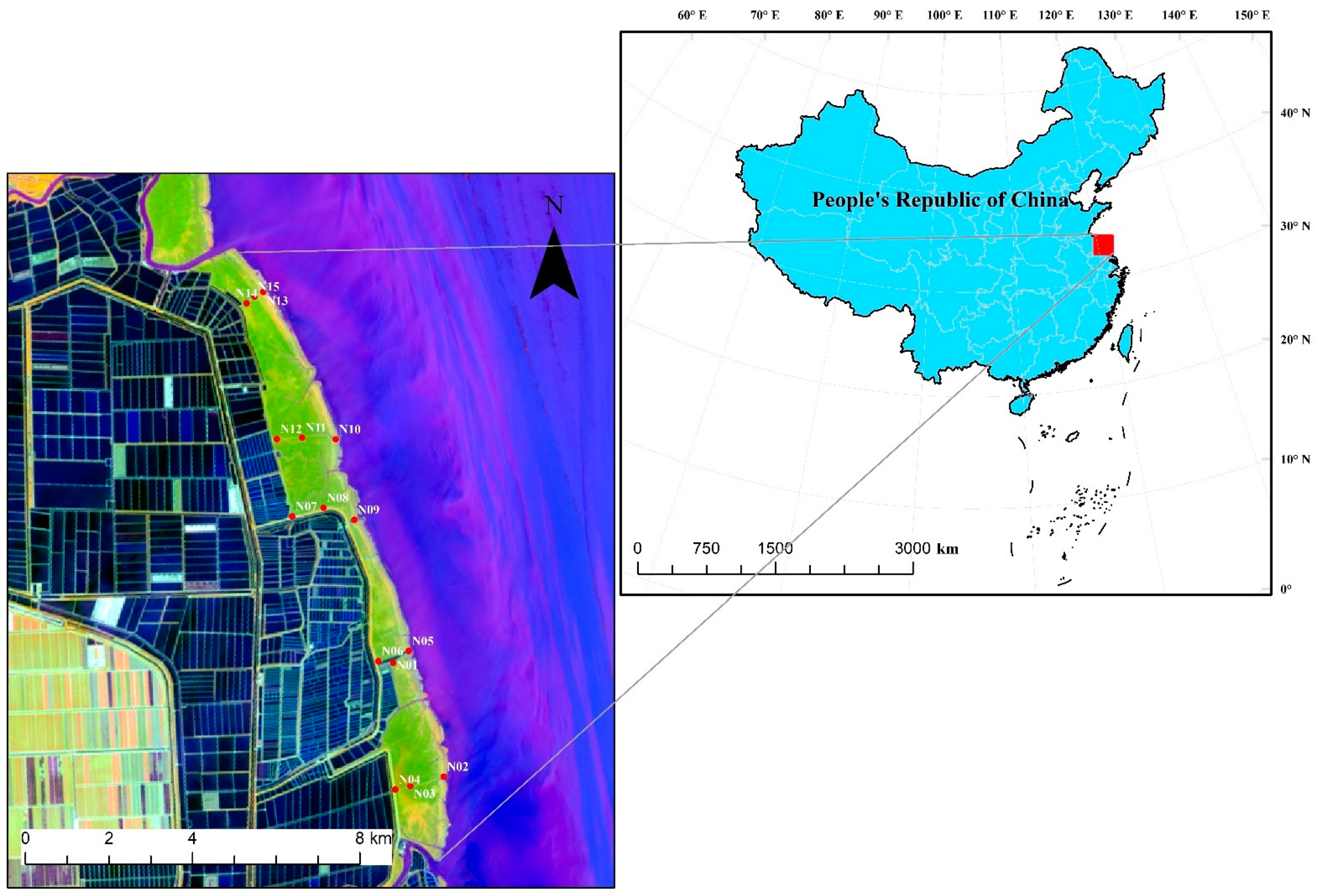
The study area is located in the coastal wetland reserves of eastern China (33°20′–33°30′ N, 120°40′–120°45′ E) and has an area of approximately 17 km². This area has a subtropical monsoon climate, with sufficient illumination and abundant rainfall. The precipitation is 980~1070 mm annually, and the annual average temperature is between 13.7 and 14.6 °C. According to the World Reference Base, the soil in the study area is Gleyic Solonchaks. Spartina alterniflora, as a strong exotic species across the world, was introduced into China in 1979. Because of its wide adaptability and strong reproductive capabilities, the population of S. alterniflora has become the most serious exotic invasion in the salt marshes of coasts in China. Nowadays, S. alterniflora has occupied most of the wetlands in the study area, replacing Suaeda salsa as the pioneer plant community on the coasts of southeastern China, and has gradually formed the single dominant vegetation community in the introduced area.

Soil sampling was conducted in 2017. We designed a stratified random sampling strategy using a space-for-time substitution method. This method allowed us to analyze the characteristics temporally using a set of spatial data for different ages of the S. alterniflora community and assisted in the investigation of the relationships between soil and invasion processes using a finite sample size. In this study, the settlement stage (i.e., (2000, 2004, 2010 and 2016) of the S. alterniflora community was initially identified using time series Landsat thematic mapper satellite images obtained from the US Geological Survey by visual interpretations. Then, we randomly selected 15 sampling sites alongside the five seaward transects according to pre-identified settlement stages. Given that the root system of mature exotic plants may well reach 1 m, a soil profile at each sampling point was excavated up to 1 m depth, and soil samples were taken from three fixed-depth intervals (0–30, 30–60 and 60–100 cm). The location and distribution of the sampling sites is presented in Figure 1.

2.2. Data Source and Processing

This paper explores the interactions between soil and S. alterniflora using remote sensing data. Therefore, plant invasion data, including the normalized difference vegetation index (NDVI) the years of introduction and soil ontology data, including the soil depth, soil properties and Sentinel-1 remote-sensing data, are needed.

2.2.1. Plant Invasion

In order to further figure out the potential effects of the invasion processes on soil functions, the precise ages of the S. alterniflora in selected sites were further identified by overlaying the 15 sampling sites to the yearly time series Landsat 5/7/8 images during 1998 and 2016. This was processed in ArcGIS 10.0. These could virtually represent the temporal factor of soil formation at each location with the satellite images.

From the Google Earth Engine platform, a product at a resolution of 250 m was obtained. It combined an 8-day normalized difference vegetation index (NDVI) based on the moderate-resolution imaging spectroradiometer. NDVI values were utilized to demonstrate the variation in plant productivity spatially, which is essential for quantifying the invasive intensity. For the sake of complete data acquisition, the average NDVI value at each sampling site was derived from the growing season (from April to September) of 2017.

2.2.2. Soil Properties and Soil Quality Index Calculation

As we all know, soil functions could often be evaluated by soil properties because of the difficulty in measuring functions directly. In general, the structural support function could be evaluated through Bulk density (BD) and the soil buffering capacity can be reflected by soil texture. Soil organic carbon (SOC) and TN (total nitrogen) represent carbon storage and soil nutrient, respectively. The SOC/TN (C/N) is an indicator of the equilibrium of C and N cycling, as well as the activity of soil microorganisms. The soil chemical environment and plant health can be reflected by soil pH. Soil salinity is associated with the dynamics of soil degradation in coastal saline soils. In the laboratory, we air-dried the bulk soil samples that passed through a 2-mm sieve. Seven soil chemical and physical properties, including soil organic carbon (SOC), total nitrogen (TN), SOC/TN, salinity, soil pH, particle size fraction and bulk density, were analyzed to illustrate the basic functionality of the soils. Usually, the Walkley–Black wet combustion method was a good fit to analyze the SOC concentration (g·kg⁻¹). The Kjeldahl digestion procedure was used to extract the TN concentration (g·kg⁻¹). We used the ratio of SOC to TN to calculate the C/N ratio. Electric conductivity and dry evaporation methods were utilized to measure the soil salt content (salinity, g·kg⁻¹). We measured soil pH in a soil/water solution of 1:2.5. Through a laser diffraction particle size analyzer, we analyzed the particle size fractions. A core sample which was 5 cm in diameter and 5 cm deep was dried at 105 °C to a constant mass for measuring Bulk density (BD, g·cm⁻³).

The soil quality index (SQI) was calculated in the laboratory using the seven soil properties listed above, for the purpose of effectively analyzing the comprehensive condition of the soil using a single index. In general, calculating the SQI took three steps: (i) identify a minimum dataset (MDS) of indicators which includes the most significantly related soil properties [35], (ii) score the identified properties, and (iii) aggregate the several selected scores into an integrated index [36].

(i) Identify a minimum dataset (MDS) of indicators which includes the most significantly related soil properties: Because the response of soils to specific management (e.g., plant invasion in this research) is critical for the evaluation of the soil quality [35], the selected indicators for SQI mainly rely on their sensitivity to the changes in the soil functions. Soil functions are the result of many physical and chemical soil properties, and it was proved necessary and effective to identify the most relevant properties to calculate an integrated index to represent more than one soil function, such as the soil desalinization and carbon storage in salt marshes, a homogeneous study area [36]. In this paper, properties that have a significant (p < 0.05) linear correlation with S. alterniflora Loisel age were identified.

(ii) Score the identified properties: To identify the overall trends effectively, scoring methods were taken into consideration. Three scoring methods were considered: “more is better,” “less is better,” and the midpoint of the optimum [20]. The relationship between each soil property and its corresponding function determined the shape of three forms of scoring function for different soil properties. Because of the positive effects that SOC has on the biomass accumulation, fertility and stable structure of coasts [37], the SOC contents were scored by the “more is better” system. Given that the lower the salinity is, the stronger the fertility of the plant health will be [38], the “less is better” system was used to score the soil salinity. The midpoint optimum function was more suitable for soil pH to represent the plant sensitivity to the soil buffering capacity [39]. The midpoint of the optimum method was realized through Gaussian functions to simulate the changes. The following formula shows how the “more is better” and “less is better” scores were fitted

$$\mathrm{S}=\frac{a}{\left[1+{\left(\frac{x}{x_0}\right)}^k\right]}$$

(1)

where S is the score of a soil property, a is the maximum score, and k is the slope (−2.5 for “more is better” and +2.5 for “less is better”) [40].

(iii) Aggregate the several selected scores into an integrated index: The score of the selected soil properties was calculated via the following formula

$$\mathrm{SQI}=\frac{{{\displaystyle \sum }}_{i=1}^n{S}_i}{n}$$

(2)

where S_i is the score of the ith soil factor and $n$ is the number of selected soil factors. A larger SQI value indicates a greater soil function. In this paper, the function that the SQI value represented was mainly related to the three basic soil parameters. Therefore, the stronger the capability of the soil carbon storge, desalinization and the environmental adaptability became, the greater the SQI value was. More details about the SQI calculation can be found in the study “Exotic Spartina alterniflora Enhances the Soil Functions of a Coastal Ecosystem” [36].

Furthermore, non-independent observations and aggregated data may produce biased, specious results due to violation of independence. Therefore, evaluating the probability of these errors provides researchers with sufficient evidence for detecting soil changes. Power analysis was used to illustrate the influence of the available data on the significance level of the interpretation of the linear relationship [36]. The power index was calculated in using the “pwr” package in R software. When a power index is over 80%, it is suggested that there is a high probability of detecting the significant changes.

2.2.3. Sentinel-1 and Principal Components Analysis (PCA)

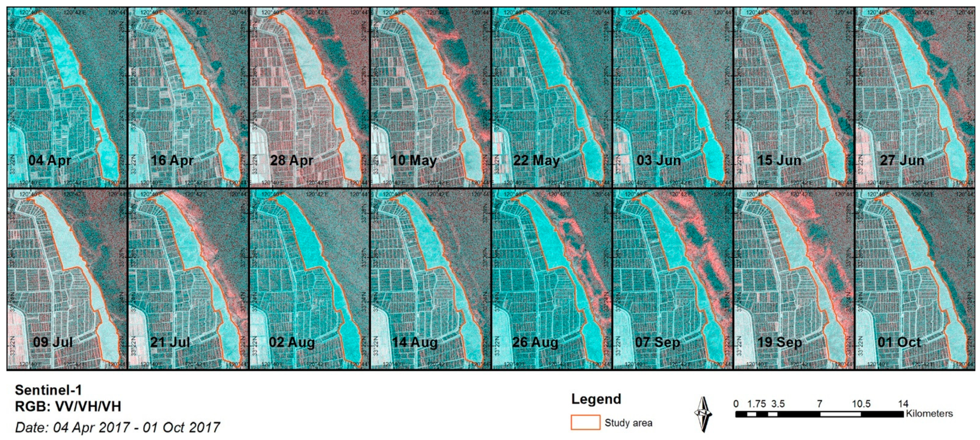
All Sentinel-1 data used in this paper can be available and downloaded freely from the Copernicus Open Access Hub (https://scihub.copernicus.eu/, (accessed on 27 December 2017)). Sentinel-1 is a near-polar solar synchronous orbit satellite (including Sentinel-1A and Sentinel-1B) and it has an advantage in providing continuous imagery with a six-day revisit time operating in the C-band instrument through the European Space Agency (ESA). In this study, only 16 Sentinel-1A scenes from 4 April 2017 to 1 October 2017 (Figure 2) were applied, as the Sentinel-1B data were unavailable during the vegetation growing period. The images of growing duration were applied because they were thought to have a greater priority than representing the vegetative variations. The selected radar images were obtained in interferometric-wide (IW) mode and were Level-1 Ground Range products.

Sentinel-1A images needed to be preprocessed in ESA’s Sentinel application platform (SNAP). A series of processing steps were realized in the platform, including Orbital Correction, Radiometric Calibration, Noise Reduction, Multilook Image Transformation to 20 m pixels and Terrain Correction. Backscatter coefficients in decibels transformed from digital pixel values were extracted from VH and VV polarizations. In order to improve the precision and stability in the time indication, the VH/VV ratio besides VH and VV polarizations was also processed for the analysis [18].

At this point, we have a total of 16 Sentinel-1A scenes with three polarization methods, totalling 48 datasets. Principal component analysis (PCA) was used for the data reduction through R software. New variables were transformed from the initial variables

$$D_{\mathrm{new}}=D\times E$$

(3)

where $D_{new}$ and $D$ are $m*n$ matrices. The new dataset $D_{new}$ includes n new variables (e.g., PC₁, PC₂, …, PCn). $D$ consists of $q$ variables, and $E$ is a $q*n$ eigenvector matrix. The new variables were selected according to the cumulative proportion of the explained variation (>85%). Only when the proportion was greater than 85% could the new dataset indicate the majority explanation of the initial dataset.

2.3. Structural Equation Model (SEM)

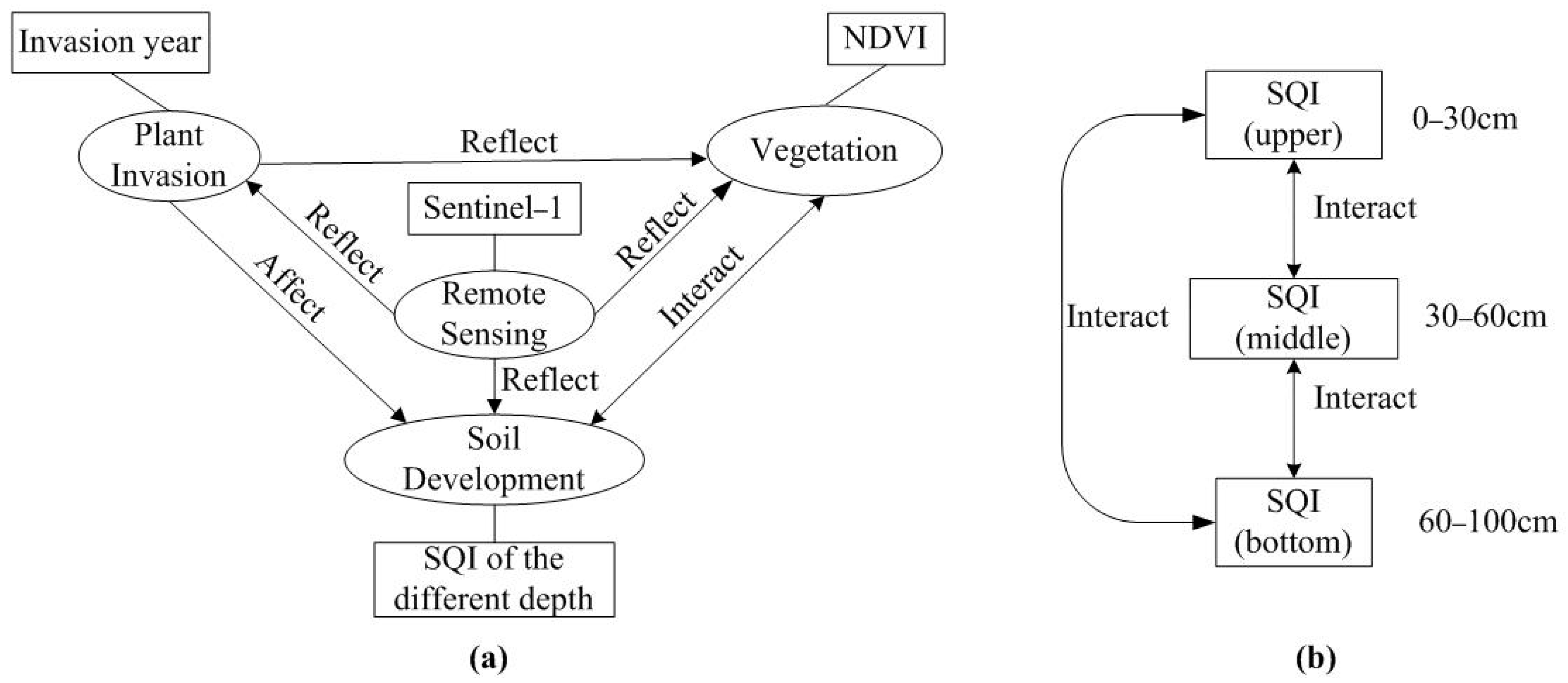
Soil development is too complex and dynamic for a simple linear method to explain the causal relationship between soil development and other objectives. These potential relationships could be combined with one or more regression equations to model soil development based on knowledge about the invasion processes, soil formation factors and the assumption of the usefulness of the remotely sensed data. SEM has the potential to be used to construct a model that can represent a complex and dynamic soil-vegetation system. Using the SEM, we designed theoretical causal relationships between the soil invasion processes and remote sensing (RS) (Figure 3a) as well as the interactions at varied soil depths (Figure 3b). In detail, the potential causal relationships between soil development, invasive plants and RS techniques linked to the observations were summarized to explore the prediction of soil development under the invasive environment conditions using remotely sensed data. In Figure 3, three relationships were constructed. First, the soils at different depths were linked because of the inner interactive mechanisms of the soil system. Second, given that vegetation is a response to plant invasion and that the soil system is adjacent to vegetation and influenced greatly by the root system of the vegetation, plant invasion, soil development and vegetation were linked. Finally, the remote-sensing method monitored the surface vegetation station, and time series RS data enabled the extraction of the plant invasion age, which represented the plant invasion process in the space-for-time substitution. Thus, remote sensing was linked to vegetation, plant invasion and soil development. In short, as shown in Figure 3, this conceptual model consisted of a set of latent variables, including plant invasion, vegetation, remote sensing and soil development, which were designed in Ellipse. All of the latent variables are represented by measured variables in rectangles. In addition, the arrow direction in Figure 3 demonstrates the relationships between the variables.

We used the lavaan R package [41] to simulate the model. Before we implemented the SEM in lavaan, the variables needed to test for univariate and multivariate normality firstly. The univariate normality was checked through the Shapiro–Wilk test and Mardia’s coefficients were used to check the multivariate normality for all variables. Next, SQI, NDVI and invasion year were log-transformed to plot with the same scale as the covariates of remotely sensed data. In lavaan, a maximum likelihood method was used to estimate the parameters. Standardized path coefficients were used to quantify all relationships. The measured variables constructed the final model, corresponding to their latent variables. At the same time, the variables could be reidentified on the basis of their p-value (p < 0.05) and modification indices (mi ≤ 5), which indicated whether a particular variable would be added or removed to improve the model [34,42].

The R² value was used to estimate the goodness of fit of the model, which demonstrated the explanation of the observed variables in the model. Besides, chi-square, the comparative fit index (CFI), the root mean square error approximation (RMSEA) and the standardized root mean square residual (SRMR) were all summarized to evaluate an overall assessment of fitness in R software.

2.4. Accuracy Evaluation

Leave-one-out cross-validation (LOOCV) was used to evaluate the predictive model. In our study, the dataset was divided into 15 groups, 14 of which were utilized as the training dataset and one as the test dataset. Three statistical metrics, including the Mean Error (ME), the Root Mean Square Error (RMSE) and the Ratio of Performance to Deviation (RPD), were used to assess the prediction accuracy. The closer the ME and the RMSE were to zero, the more accurate the predictive model was considered to be. RPD is the ratio of the standard deviation of the observed values to the RMSE of the predictions; when RPD > 1.4, the prediction accuracy was considered acceptable. These indicators were calculated as follows

$$\mathrm{ME} = \frac{1}{n}{\displaystyle \sum }_{i=1}^n\left(p_i-o_i\right)$$

(4)

$$\mathrm{RMSE}=\sqrt{\frac{1}{n}{\displaystyle \sum }_{i=1}^n{(p_i-o_i)}^2}$$

(5)

$$\mathrm{RPD}=\frac{\sqrt{\frac{1}{n}{{\displaystyle \sum }}_{i=1}^n{(o_i-\overline{o})}^2}}{\sqrt{\frac{1}{n}{{\displaystyle \sum }}_{i=1}^n{(p_i-o_i)}^2}}$$

(6)

where n is the number of sample points, $P_i$ and $O_i$ are the predicted and observed values, respectively, and $\overline{o}$ is the mean value of the observed data.

3. Results

3.1. Results of Soil Quality Index and Vegetation

Table 1. Statistical characteristics of the soil quality index.

Data	Mean	Min	Median	Max	Sd	CV
0–30 cm	0.59	0.38	0.59	0.74	0.10	16.95%
30–60 cm	0.53	0.13	0.47	0.86	0.25	47.17%
60–100 cm	0.58	0.23	0.62	0.81	0.18	31.03%
0–100 cm	0.56	0.13	0.56	0.86	0.18	32.69%
NDVI	0.23	0.07	0.24	0.33	0.08	34.76%

shows the statistical characteristics of the soil quality index and vegetation productivity at the 15 sites, showing small differences in the SQI among the depth intervals. Here, the soil quality index (SQI) was calculated from the SOC, soil pH and salinity values, which were found to have a significant relationship with S. alterniflora [36]. SOC was calculated according to the “more is better” method. For salinity, the “less is better” was applied. It is useful for the optimum function to transform the soil PH data. From the table, we found that the SQI in the study area ranged from 0.13 to 0.86, with an average value of 0.56. The entire variation in the soil profile in the upper 1 m was 32.69%, showing moderate variability. The topsoil layer at 0–30 cm ranged from 0.38 to 0.74, with the highest average value of 0.59 for this depth interval; the middle soil layer at 30–60 cm ranged from 0.13 to 0.86, with an average value of 0.53; and the bottom soil layer at 60–100 cm ranged from 0.23 to 0.81, with an average value of 0.56. Overall, the mean values of the SQI at the three depths were similar. The CV values at the three different depths were 16.95%, 47.17% and 31.03%, respectively, all belonging to the moderate variability standard. In addition, the summary characteristics of surface vegetation production, indicated by NDVI, were described as well. The NDVI in the study area ranged from 0.07 to 0.33, with an average value of 0.23. Its CV value was 34.76%.

3.2. Relationship between Invasion Process and Soil Quality Index

We analyzed the relationship between the invasion year and SQI at different depths through Person’s correlation analysis and power analysis. From

Table 2. Correlation between the invasion time of S. alterniflora and the soil quality index at the three different depths.

Data	Pearson’s r	p-Value	Power
0–30 cm	0.907	<0.01	1
30–60 cm	0.717	<0.01	0.89
60–100 cm	0.546	<0.05	0.59
NDVI	0.653	<0.01	0.79

, we found that SQI values at three depths and NDVI were all positively related to the invasion year of S. alterniflora (p < 0.05). The analysis of the heterogeneity of the SQI values found that the soil quality in the research area had a slightly high correlation with the invasion year in the 0–30 cm layer. The Pearson’s r value was 0.907 (p < 0.01). The Pearson’s r values at 30–60 and 60–100 cm were 0.717 and 0.546, respectively, which were moderately correlated with the invasion year. From the perspective of soil depths, it can be concluded that as the depth increases, the resulting correlation value decreases trend. The results show that the Pearson’s r for the NDVI value was 0.653, showing medium correlation with the invasion year. In the meanwhile, the power index of SQI in the 0–60 cm was over 80%, and NDVI was almost near to 80%, showing a moderate probability of detecting the significant changes.

3.3. Predictors Selection and Modeling

In this paper, the 10 principal components, selected according to the principal component analysis method, were used as the new prediction variables that participated in model construction, with a cumulative explanation proportion of 89.10%. From the results, 10 of the prediction factors were eliminated in the construction process because of their poor p-values when simulating the processes (Figure 4). Yang et al. [18] provide details about the analysis of the physical meaning of the PCs.

Based on prior knowledge of the invasion processes and soil development characteristic in coastal wetlands, this paper constructed a mechanistic model that explored the interactive relationship between soil development and plant invasion with the assistance of a remote-sensing approach by using soil-quality data, invasion vegetation data and 10 new predictive factors that passed a single-variable normal distribution test. In the SEM, the model explained 86.2% of the variations that occurred during the invasion years, 45.2% of the NDVI variability, 95.9% of the SQI variability in the top layer, 92.7% of the SQI variability in the middle layer and 49.7% of the SQI variability in the bottom layer. The results indicated that the structural equation model was a reasonable and efficient method to simulate wetland soil development using ancillary data, such as information on invasion and remotely sensed data.

In addition, quantitative results among the observed variables were obtained. The impact of the invasion age on NDVI was 0.673, and the NDVI value in the model was only determined by the invasion age. At the same time, the NDVI value played a negative role in forming the surface SQI at 0–30 cm, with an influence coefficient of −0.302. Moreover, it is easy to observe that the invasion process participates in the simulation of the above two soil layers, playing an important role in soil development at the 0–60 cm depth interval, and the coefficients were 0.992 and 0.709. From the prospect of depth, the SQI at 0–30 cm was affected by the SQI at 30–60 cm with a standard coefficient value of 0.254, which also exerted positive impacts on the SQI at 60–100 cm with an influenced coefficient value of 0.705.

Considering that soil development is a multifactorial and dynamic process and soil quality assessment requires numerous physicochemical and biological factors, correlations between the invasion time of S. alterniflora and the specific chemical and physical soil properties at the three different depths were also analyzed (

Table 3. Correlation between the invasion time of S. alterniflora and the specific soil properties at the three different depths. Statistically significant (at 0.05 level) values are shown in bold.

Depth		SOC	TN	C/N	pH	Salt	BD	Clay	Silt	Sand
0–30 cm	r	0.81	0.43	0.35	0.66	−0.83	−0.38	−0.38	−0.40	−0.43
	p	<0.01	0.11	0.20	<0.01	<0.01	0.17	0.16	0.14	0.11
	power	0.98	0.37	0.26	0.81	0.99	0.29	0.3	0.33	0.37
30–60 cm	r	0.28	−0.23	0.44	0.46	−0.74	−0.34	−0.12	−0.45	0.33
	p	0.32	0.41	0.10	0.09	<0.05	0.22	0.68	0.09	0.23
	power	0.17	0.13	0.38	0.42	0.93	0.24	0.07	0.41	0.23
60–100 cm	r	0.23	0.33	−0.13	0.22	−0.52	−0.19	0.22	0.39	−0.36
	p	0.42	0.23	0.63	0.42	<0.05	0.51	0.43	0.15	0.19
	power	0.13	0.23	0.08	0.13	0.55	0.1	0.13	0.32	0.27

). From Table 3, we could find that there was a significant correlation between the invasion year and SOC, pH and salinity in the upper 30 cm. In addition, only salinity was related to the invasion year in the 30–100 cm. This is consistent with the results in the pathway results. As well, power analysis results also show that only SOC, pH, salinity in the 0–30 cm and salinity in the 30–60 cm were >80%, with a high probability of detecting significant changes.

3.4. Validation

Table 4. Validation statistics of the mechanistic model.

Depth (cm)	ME	RMSE	RPD
0–30	−0.06	0.09	1.21
30–60	0.02	0.16	1.50
60–100	0.01	0.14	1.23
0–60	−0.02	0.13	1.44
30–100	0.01	0.16	1.38
0–100	−0.01	0.14	1.35

presents the values of ME, RMSE and RPD that resulted from the leave-one cross validation, revealing a successful model for SQI prediction in summary, especially for soils at a depth interval of 0–60 cm. The RPDs of the SQI in the middle layer and the upper 60 cm were 1.50 and 1.44, respectively, and the RMSEs were 0.16 and 0.13, respectively, showing the predictive capacity of the SQI in the upper 60 cm with the SEM model. The predicted and observed SQIs from the cross validation are plotted in Figure 5. The predicted values were in good accordance with the observations, with an R² value of 0.47 and an RMSE of 0.14 (Figure 5d and Table 4). For the three depth intervals, the R² values are 0.59 at 0–30 cm, 0.57 at 30–60 cm and 0.31 at 60–100 cm. Among them, the SQI in the middle layer was insignificant (p = 0.12).

4. Discussion

4.1. Relationships between Soil Quality Index and Invasion

In this paper, seven soil properties were considered to calculate the soil quality index (SQI). However, only three soil properties, soil organic carbon (SOC), soil pH and salinity, were selected to indicate the comprehensive soil functions because these three properties were proven to be significantly related to the soil functions [36]. From the results, we discovered that the SQI values at the three depths were similar, illustrating that the SQI is an ideal index to represent the overall conditions of the soils. This was supported by several scholars who have pointed out the possibility of using a singular index to effectively inspect the overall soil condition [20,40]. Given that the SQI consisted of SOC, soil pH and soil salinity, the SOC usually represents carbon sequestration, soil pH and soil salinity are closely related to the optimal growth environment, the SQI in this paper represents the mutual interactions between several soil processes. In previous studies, exotic plants have been shown to influence soil quality in the top 60 cm [36,43]. In this paper, it was proven that the introduction of exotic plants had an effect on the soil function and development of the whole soil profile in the upper 100 cm, enabling us to better understand the interactions between the invasive processes and the soil system in the study area.

The results also illustrated the significant positive relationship between the invasion time and the SQI in the upper 100 cm, especially in 0–30 cm. This is mainly because the invasion processes have a positive effect on SOC and soil pH, while soil salinity was weakened with the plant invasion. This suggests that the invasive S. alterniflora exerted a positive influence on soil functions on coasts by improving the living environment, strengthening the capability of carbon storage and desalinization. The substantial and effective control of S. alterniflora on sea water and salinity may help improve the soil quality [17,36], and it has a high level of above- and belowground biomass, leading to an increase in the organic carbon stocks in the soils [44,45,46]. In view of the depth intervals, the larger the depth was, the less significant the correlation was. This suggests that topsoil development was sensitive to the invasion of S. alterniflora. This could be because the biological and hydrological processes in the surface layer had been affected for a longer time, in contrast with the other two deeper layers, after the new species was introduced [10,47,48].

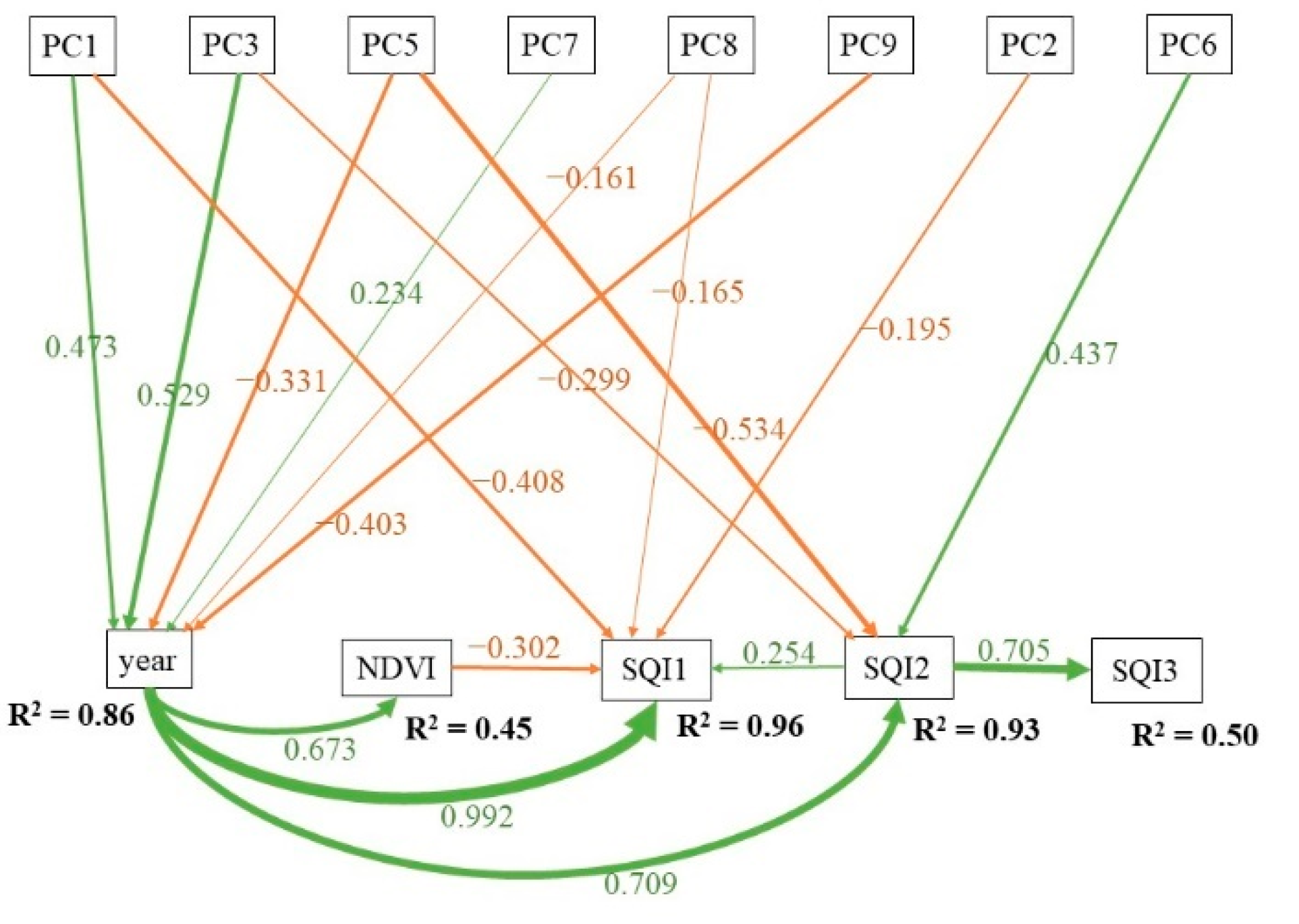
In addition, the quantitative relationships not only further confirmed that the invasion process enhanced the soil quality, especially at the 0–60 cm depth range, but also suggested that the vegetation introduced by the invasive plant weakened the development of soil quality, consistent with the findings that the invasion of S. alterniflora has a negative impact on the ecology of coastal wetlands [9,10]. This is because NDVI was closely related to the growth of S. alterniflora, and marshland vegetation prefers higher salinity, which could aggravate soil salinization, resulting in worse soil quality.

Furthermore, the importance of the interaction between soil development and the invasion process was highlighted. We found that, in contrast with the surface vegetation represented by NDVI, the development of the upper two soil layers in the 0–60 cm layer possessed a greater relationship with the invasion process. The direct contribution of the plant invasion might be mediated by the inherent linkage of soil development extents between different layers, while the invasion process influenced soil development. This suggests that invasion processes show a great potential for improving soil quality and promoting soil development.

4.2. Possibilities of Mechanistic Soil Modeling with Remote Sensing

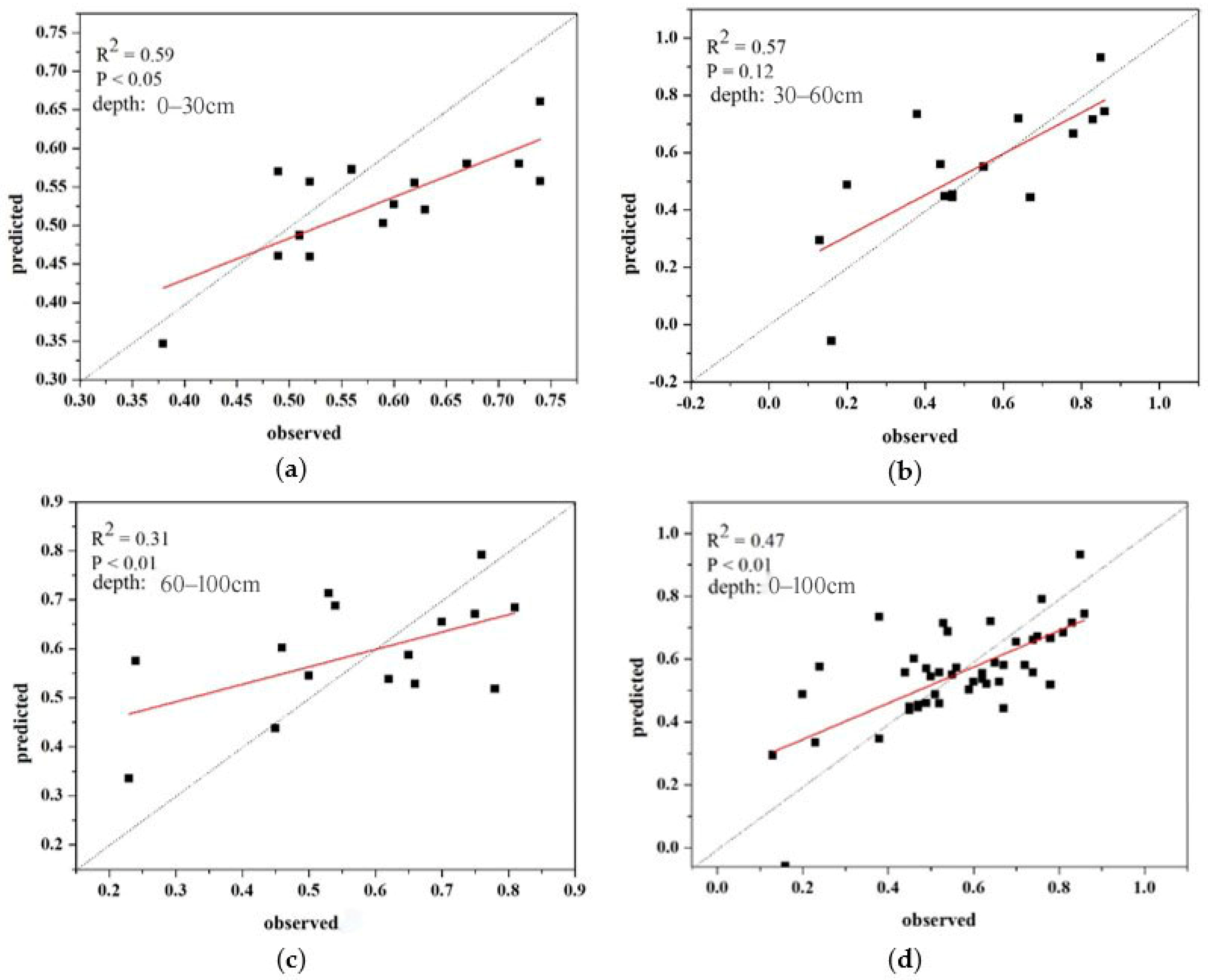
The results show that the level of accuracy of the soil quality index estimations from the Sentinel-1 images using the simulated dataset could be classified as “intermediate” in the upper 60 cm (RPD > 1.4) [30], with an RMSE value of 0.13. Earlier studies have proved that the prediction model based on remote sensing techniques was effective in simulating the soil properties [27,30]. Considering that these results were from the finite selected soil properties and multiple remote-sensing data sources, resulting in the introduction of uncontrolled error factors, the potential for a quantitative estimation of the soil quality index from satellite sensors appears to be rather limited. The identification of soil quality in the upper 60 cm was considered to be a success for the soil development simulation. From the results, the accuracy of the soil quality estimation in the middle layer at a depth of 30–60 cm was relatively higher than that at the 0–30 cm and 60–100 cm depth intervals. Figure 4 illustrates that the soil in the 30–60 cm layer had a direct effect on the topsoil and bottom soil, while the soils in the other two layers might explain why the RPD of the middle soil was superior to that of the other two depth intervals.

Traditionally, soil properties and remote-sensing predictors have been analyzed as two singular variates. The results suggested that the invasion year was highly and significantly correlated with the soil quality indices (Table 2), indicating that the effects of S. alterniflora on soil systems could be represented by the soil observations. In this study, our focus was always on the soil-vegetation system, including the combined soil quality at different depths, as a whole, in terms of its multiple interactive influences, rather than isolating the processes from the system. This greatly benefited from the ability to detect the characteristics of the short-term variation in dense vegetation cover [23,24,49].

Regarding the Sentinel-1 data, they mainly provide services for monitoring sea ice and Arctic environment, ground deformation (such as earthquake, landslide, land subsidence and volcanic activity), forest fire and flood management, water management, soil protection and humanitarian assistance. In earlier studies, the potential of Sentinel-1 in vegetation monitoring was recognized, such as interpreting wetlands and mapping grasslands [21,29,50]. In addition, it has been found that radar imaging is greatly useful to delineate flood boundaries beneath dense vegetation canopies [23]. In the coastal regions, the cloud-free multispectral is frequently unavailable, meaning it is difficult to obtain optical remote sensing of wetlands. Synthetic aperture radar (SAR) offers tremendous potential to identify, monitor and map wetlands with vegetative coverages due to the ability to operate day and night and penetrate clouds. From the results of our study, Sentinel-1 imagery was proven to have potential for the detection of areas with dense vegetation and was useful for simulating soil development.

In our study, the SEM model was so promising that it had the ability to capture the latent interactions between the invasion vegetation and SQI at different depths combined with knowledge on invasion processes. Contrary to empirical models, mechanistic models usually construct relationships according to the inherent mechanism of their objects. Through SEM, the relationship was analyzed not only qualitatively but also quantitatively.

4.3. Limitations and Implications

In this paper, we have demonstrated the reliability of the SQI method, the advantage of using SEM to simulate soil development with plant invasion, and the potential of applying Sentinel-1 data to study soil quality and development. This paper demonstrates a crucial attempt to use an integrated index representing the comprehensive soil functions to model soil–vegetation interrelationships through Sentinel-1 images. These results might contribute to large-scale applications and provide a more technical index and cost-efficient method for describing these interactions.

Nevertheless, there were only a few properties selected to calculate the SQI, which decreased the comprehensiveness of the integrated indicator. More soil properties should be considered, especially the factors that relate to the chemical, physical and biological processes. Moreover, although SEM has great potential in analyzing finite samples, obtaining more effective samples could improve the accuracy of the model. In addition, multisource remotely sensed data should be considered for joint use in the future, as they could improve the quantification of vegetative variability.

5. Conclusions

Under constant S. alterniflora invasion, the characteristics of soil quality at different depths have varied. There are several conclusions of this study to summarize. First, the soil quality index values at different depths exhibited some influential trends during invasion. Overall, the introduction of invasive plants could strengthen coastal salt marsh functionality. The topsoil was severely influenced. Second, the construction of the SEM model supported the assumption of causal relationships between soil–vegetation–RS at a local scale. Third, remotely sensed data showed great potential in predicting soil quality under dense vegetation, especially in the upper 60 cm. In summary, this paper aimed to construct a mechanistic method to study coastal soil quality effectively and conveniently using a comprehensive indicator with the aid of remotely sensed data, thus assisting in the development and implementation of coastal management strategies at a small and local scale.