An Object-Based Approach for Mapping Tundra Ice-Wedge Polygon Troughs from Very High Spatial Resolution Optical Satellite Imagery

Abstract

Very high spatial resolution commercial satellite imagery can inform observation, mapping, and documentation of micro-topographic transitions across large tundra regions. The bridging of fine-scale field studies with pan-Arctic system assessments has until now been constrained by a lack of overlap in spatial resolution and geographical coverage. This likely introduced biases in climate impacts on, and feedback from the Arctic region to the global climate system. The central objective of this exploratory study is to develop an object-based image analysis workflow to automatically extract ice-wedge polygon troughs from very high spatial resolution commercial satellite imagery. We employed a systematic experiment to understand the degree of interoperability of knowledge-based workflows across distinct tundra vegetation units—sedge tundra and tussock tundra—focusing on the same semantic class. In our multi-scale trough modelling workflow, we coupled mathematical morphological filtering with a segmentation process to enhance the quality of image object candidates and classification accuracies. Employment of the master ruleset on sedge tundra reported classification accuracies of correctness of 0.99, completeness of 0.87, and F1 score of 0.92. When the master ruleset was applied to tussock tundra without any adaptations, classification accuracies remained promising while reporting correctness of 0.87, completeness of 0.77, and an F1 score of 0.81. Overall, results suggest that the object-based image analysis-based trough modelling workflow exhibits substantial interoperability across the terrain while producing promising classification accuracies. From an Arctic earth science perspective, the mapped troughs combined with the ArcticDEM can allow hydrological assessments of lateral connectivity of the rapidly changing Arctic tundra landscape, and repeated mapping can allow us to track fine-scale changes across large regions and that has potentially major implications on larger riverine systems.

1. Introduction

Permafrost-Earth materials that remain at or below 0 °C for at least two consecutive years underly approximately 24% of the exposed land surface of the Northern Hemisphere [1]. Permafrost landscapes are warming across the Arctic [2] and this is coupled with increased socioeconomic development [3,4]. Areas with ice-rich permafrost are especially vulnerable to destructive processes of ground-ice degradation, such as thermokarst and thermal erosion. Thawing ice-rich ground, especially in cold permafrost areas, is challenging geosystem and ecosystem services [5]. Thawing of ice-rich permafrost increases lateral biogeochemical fluxes [6,7,8] and release of soil carbon to the atmosphere [9]. It also alters coastal marine ecosystems [10], geomorphology [11,12,13], vegetation [14], and hydrology [15]. Ice wedges are indicative of cold permafrost [16] and are ubiquitous ground-ice features in the continuous permafrost zone, forming polygonal networks characteristic of the vast lowland Arctic regions [17]. Vegetation and geology maps suggest that about 40–70% or more of the Arctic landscape is occupied by polygonal ground [18,19], but the exact extent is largely unknown. Ice-rich permafrost terrain in Arctic regions typically includes several meter-wide ice wedges that form as a result of thermal contraction cracking in the winter and subsequent infilling with snowmelt in the spring repeated over centuries to millennia [20,21,22].

Morphometrically, ice-wedge polygons are pronounced on the landscape by networks of discontinuities formed by ice-wedge troughs and/or linear ridge features (rims) framing polygonal centers of low, flat, or high. Ice-wedge polygons typically vary in size from 10 to 30 m across. As ice wedges grow, low-centered polygons framed by elevated rims form as a result of deformations of ice and soil caused by pressure from growing wedges. Low-centered polygons often contain intra-polygonal ponds. At the stage of active ice-wedge development, ice-wedge troughs are hardly visible or very shallow. Any wedge-ice melt increases trough depth and the lateral hydrological connectivity among troughs. Eventually, this results in the formation of high-centered polygons with elevated centers and well-developed troughs over partially degraded ice wedges [23,24]. Active degradation of ice wedges commonly leads to the formation of deep (>1 m) and wide (up to 10 m) pits and troughs; within poorly drained terrain, these depressions are usually filled with water. Pits and troughs are the most characteristic thermokarst landforms in polygonal landscapes [25,26]. Under certain conditions, initial pits and troughs may develop into large thermokarst ponds and lakes [27,28] though such transitions in the areas with cold continuous permafrost are still relatively rare.

Degradation of ice wedges is a quasi-cyclical process, with degradation often occurring over a shorter time scale than aggradation; stabilization of recently degrading wedges occurs as a result of accumulation of soils and organic matter in ice-wedge troughs [28,29]. The microtopography associated with polygonal tundra affects Arctic ecosystems from local to regional scales, due to its impacts on the flow and storage of water [23], vegetation [30], accumulation of organic carbon [31,32], and ground temperatures [33,34]. Over recent decades, widespread ice-wedge degradation has been documented at numerous locations across the Arctic tundra in the field and through remote sensing techniques [23,29,35,36,37]. Ice-wedge degradation strongly affects the environment and is extremely hazardous for infrastructure; it may be triggered by climatic fluctuations [23,33], wildfires [35], human activities [4], or other factors that may lead to an increase in active-layer thickness. Resolving deep ice-wedge trough occurrence and dynamics is critical for detecting ice wedge degradation and in turn characterizing and understanding future permafrost landscape behavior [29]. Techniques have been developed for mapping ice-wedge polygons and estimation of volumes of wedge ice [38,39,40,41,42], but techniques to map ice-wedge troughs specifically over large areas are lacking. Ice-wedge trough mapping can allow a more accurate estimation of ground ice distribution and volumes [28] as well as surface water connectivity. Studies have detected ice-wedge degradation in the absence of ponding [34,35], therefore the ability to map and detect micro-topographic changes in troughs will refine estimations of thermokarst extent. Improvements in resolving ice wedge trough and polygon centers using remote sensing data will also contribute to a better spatial representation of ground thermal regimes in permafrost regions [34]. Furthermore, being able to detect and map ice-wedge trough subsidence will enable a better understanding of the impacts and ecosystem responses [33] of current and future ice-wedge degradation. The current lack of mapping and, therefore also knowledge, of fine-scale morphodynamics of polygonal landscapes introduces uncertainties to regional and pan-Arctic estimates of carbon, water, and energy fluxes [23,43,44].

The limited utilization of VHSR imagery in Arctic science products is partly due to prevailing knowledge gaps in sophisticated image analysis methodology, which can effectively cope with the complexities of VHSR satellite imagery [42]. The ice-wedge polygon landscapes are difficult to characterize in any remote sensing imagery of spatial resolution coarser than 4 m [45]. Studies have emphasized the need for spatial details to accurately detect and characterize ice-wedge polygons and their associative elements, such as troughs and rims. In this context, VHSR satellite imagery holds great promise for accurate delineation of morphometric characteristics over large geographic domains. In the past, the VHSR data availability across the entire Arctic domain and the associated cost have had been the main challenges in pan-Arctic mapping applications. However, in recent years, the entire Arctic has been imaged by the VHSR commercial sensors owned by DigitalGlobe (now known as Maxar) for nearly six times. The imagery is freely available to United States National Science Foundation-funded researchers. Visual inspection and manual digitization of VHSR imagery have widely been used in mapping micro-topographic features to understand morphological dynamics [46] at the expense of time/labor and with limited spatial extent. Traditional per-pixel-based algorithms are fundamentally challenged by sub-meter-resolution imagery [47]. Increasing spectral heterogeneity in VHSR imagery leads to fewer class variances of the conventional per-pixel-based algorithms, which make it very difficult to accurately resolve fine-scale features, such as troughs and rims [48,49]. The GEographic Object Based Image Analysis method (GEOBIA, or OBIA) [47,50] has proven to be one of the most powerful innovations in a contemporary paradigm of remote sensing for analysis of very high spatial resolution imagery, as well as for harmonizing other remote sensing data products [51,52]. Many argue that, to a certain extent, GEOBIA attempts to mimic the cognitive processes that humans utilize in image interpretation, either replicating and/or surpassing the accuracies of expert interpretations via semi- or fully automated workflows [47,50,53,54]. GEOBIA has been successfully used in conventional remote sensing-based land cover mapping applications, as well as in a broad spectrum of interdisciplinary studies, including mapping refugees in east Africa [55], documenting penguin guano in Antarctica [56], mapping dunes on Mars [57], and extracting archeological features [58].

The central objective of this exploratory study is to develop a GEOBIA-based methodological framework, which links low-level motifs and domain knowledge, to automatically extract ice-wedge polygon troughs from VHSR commercial satellite imagery. We further perform a systematic experiment to understand the degree of interoperability of knowledge-based workflows across tundra vegetation units focusing on the same semantic class. In a broader context, this study relates to our on-going work on developing a mapping application for Arctic permafrost land environments (MAPLE) [42,59,60], which aims to leverage imagery-enabled science products for Arctic earth science applications.

2. Materials and Methods

2.1. Data and Study Area

We selected two candidate commercial satellite scenes from the North Slope of Alaska (Figure 1) representing two distinct tundra vegetation units. The Polar Geospatial Center (PGC) at the University of Minnesota provided the radiometrically corrected, orthorectified imagery, which were acquired in July 2010 (site 1) and July 2015 (site 2) by the Worldview-2 (WV2) commercial satellite sensor. The WV2 hyper-spatial sensor records the panchromatic (PAN) and eight multispectral (MS) bands with a ground sampling distance of ~0.46 and ~1.84 m at nadir, respectively, with 11-bit radiometric resolution.

The WV2 scene from site-1 comprises a sedge tundra-dominant wetland landscape (CAVM, [19]), with low-centered ice wedge polygons, where the polygon center is characterized typically by water impoundment. The WV02 scene of site-2 primarily comprises tussock tundra and troughs indicative of actively degrading ice wedges or ice wedges that degraded in the past but that are no longer actively degrading. Site 1 is located in a marine silt terrain unit with a high ground ice content, whereas site 2 is located in a marine sand and silt terrain unit with a moderate ground ice content [25]. Both regions exhibit a mosaic of land surfaces that have been reworked by thermokarst lake processes, which have resulted in the formation of numerous vegetated drained thaw lake basins (DTLBs), with characteristic epigenetic ice wedges and interstitial residual primary surfaces of the Arctic Coastal Plain with larger ice wedges. The dimensions and size of ice wedges here depend mainly on the age of the vegetated land surface—the older, the higher the likelihood of large ice wedges.

Wedge-ice volume in the upper permafrost of the primary surface varies from 4% to 28% (13% average, 26 sites), while in DTLBs of the Arctic Coastal Plain, the ice volume ranges from 1% (young basins, 3% average, 6 sites) to 22% (old basins, 11% average, 13 sites); the average wedge-ice volume for all studied drained-lake basins (19 sites) is estimated to be 8% [17]. The average size of polygons on the primary surface was 14 m, while in young and old lake basins, it was 33 and 18 m, respectively. Low-centered ice-wedge polygons (Figure 1A) prevail mainly within young DTLBs and flood plains, while high-centered polygons (Figure 1B) may be observed mainly within remnants of the primary surface and oldest DTLBs. Polygons that represent a transition from low- to high-centered are also common in DTLBs of various ages that have experienced recent ice-wedge degradation.

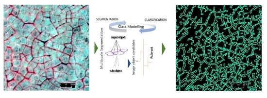
2.2. Methodological Framework

Unlike in traditional per-pixel-based image classification, which solely sits on the brightness values of individual pixels, the GEOBIA considers groups of pixels that form homogenous objects. In general, this object resembles real-world entities. The success of GEOBIA relies on its prime design goal of meaningfully grouping pixels (rather than treating them as single entities) by cross-pollinating spectral, textural, geometric, topological, and contextual information. The GEOBIA utilizes a cohesive methodological platform for machine-based characterization and classification of spatially relevant real-world entities, incorporating multiscale regionalization techniques augmented with nested representations and rule-based classifiers [61,62,63]. This kind of integrated framework, linking the concept domain and digital domain, is vital in landform mapping [64], because the imagery-based feature extraction can be supplemented and guided with expert knowledge [65]. Fundamentally, GEOBIA sits on two pillars: segmentation and classification. The former involves the creation of image objects using segmentation algorithms, whereas the latter attempts to semantically map “image” objects to “real-world” objects [58]. Overall, re-segmentation and re-classification provide an expert-based iteratively refining model for the semantic classes in question. Figure 2 illustrates our multi-scale trough modelling workflow. The ultimate goal is to create a meaningful link between low-level features (defined on image object candidates) and high-level semantics (class labels) in the image via multiscale segmentation and knowledge-based rulesets.

2.3. Data Processing

We subjected the candidate WV02 imagery to mathematical morphological operations to highlight the trough objects prior to the segmentation process. Our goal was to use morphological filtering as a means of attenuating the other objects present in the image and providing additional cues to effectively operate the segmentation algorithm. This will yield image segments (image object candidates) with meaningful correspondence to real-world objects. From a theoretical standpoint, mathematical morphology (MM) explores the geometric structure of an image in a nonlinear fashion [66,67]. MM is a well-established stand-alone image analysis framework with its own application opportunities and challenges [68,69,70,71,72]. Witharana et al. [58] demonstrated the practicality of MM operations as pre-processing instruments in object-based image analysis. Erosion and dilation are the most fundamental operations in morphological image processing. While the former erodes the bright areas of the image and expands the dark zones, the latter dilates the bright areas and shrinks the dark areas. Top-hat and black-hat transforms are a combination of basic operations. The former involves subtraction of an opened image from the original image. This process identifies points of high curvature [67]. The latter (the complement of the former) identifies dark objects surrounded by bright objects. Gradient is another MM operator that is useful for finding the outlines of structures. Based on a series of MM filtering operations, we selected erosion, top-hat, black-hat, and gradient as useful operators to create filtered images from the original WV02 images.

2.3.1. Image Segmentation

We utilized two segmentation algorithms: (1) multiresolution segmentation and (2) multi-threshold segmentation, which are available in the eCognition Developer (Trimble Geospatial, Munich) software package. The conceptual basis of the above algorithms is well addressed in the literature, therefore we will only briefly describe the candidate segmentation algorithms. Multiresolution segmentation (MRS, see [73]) is a relatively complex image- and user-dependent algorithm [54,74,75,76]. The MRS algorithm iteratively merges pixels based on homogeneity criteria driven by three parameters: scale (s), shape, and compactness [77,78], of which the scale parameter is considered the most important [79,80]. The multi-threshold segmentation (MTS) algorithm couples histogram-based methods and the homogeneity measurement of multiresolution segmentation to calculate a threshold dividing the selected set of pixels into two subsets, whereby the heterogeneity is increased to a maximum [56,81]. The MTS algorithm operates on the image object domain. It splits the image objects and classifies resulting child objects based on a pixel value threshold. The user can define the pixel value threshold, or it can operate in a self-adaptive manner when coupled with the automatic threshold algorithm (ATA) in eCognition Developer [81]. The ATA initially calculates the threshold for the entire scene, which is then saved as a scene variable, and made available for the MTS algorithms for segmentation. Subsequently, if another pass of segmentation is needed, the ATA calculates the thresholds for image objects and saves them as object variables for the next iteration of the MTS algorithm.

2.3.2. Trough Modelling Workflow

The first phase of the trough modelling workflow (Figure 2) involves the derivation of secondary products from the candidate imagery and integration of existing GIS/thematic layers, such as coarse-scale land cover data. Subsequently, the segmentation takes place in a multiscale fashion. A coarser level segmentation that operates on existing thematic layers handles the removal of large non-targets, for example, water bodies. The remainder of the scene is further decomposed into a hierarchy of super-/child-image objects. Likewise, the scene is systematically exposed to a class modelling process [82], the first cycle of which progressively decomposes the input image layers into meaningful image object candidates, and the remaining cycles perform class-/object-specific segmentation. Subsequently, the remote sensing quantification (low-level image attributes) of image object candidates and the domain knowledge of permafrost polygonal landscapes were interfaced via a fuzzy rule-based system. We used the candidate scene from site-1 (sedge-dominant) to build the master ruleset [83] and later repurposed it for the candidate image scene from site-2 (tussock dominant) to explore the portability of the master ruleset.

The MRS algorithm with a large-scale parameter (s = 50), which is a unitless parameter that controls the size of the image segments [75], was run over the multispectral imagery (with all bands) to produce coarse segments (Level 0 (L0), Figure 2). We used the normalized difference water index (NDWI) to remove water objects before proceeding to the next level of segmentation. The remaining coarser segments (super-objects) were then re-segmented to smaller objects (sub-objects) based on the black-hat image using the MTS algorithm. This step produced level 1 segments (L1, Figure 2). The thresholds for the MTS algorithm were automatically adapted from local statistics of the super-objects (black-hat image) rather than based on global (scene-wide) statistics. This process successfully yielded small seed segments with acceptable correspondence (size and shape) with trough morphometry. At this level (L1), we used image object properties (spectral, geometrical, and spatial) to extract trough-like objects. Of the plethora of properties, we narrowed it down to a set that best describes trough-like objects; those include the mean difference from the super object, area, density, and radius of the smallest enclosing ellipse [81]. The standard deviation of the gray-level co-occurrence matrix (GLCM) was calculated as an object variable for the non-trough objects and used as an indicator to filter out texturally homogeneous objects. The remaining object domain (non-trough objects) was subjected to another re-segmentation cycle, based on the black-hat image using the MRS algorithm and a smaller scale parameter (s = 5). This process re-partitioned the image objects (super-object) from the previous level (L1) and produced another layer of sub-objects at Level 2 (L2, Figure 2). We then used the mean ratio to super object and density as two key properties to extract trough-like objects.

Finally, we assessed the classification accuracies of our automated detection based on manual detection. We randomly placed 100 × 100m grid cells in the study areas to sample automated and manual detection. Quantitative error analysis comprised correctness (Equation (1)), completeness (Equation (2)), and F1 score (Equation (3)). The correctness and completeness measures gauge the commission and omission errors, respectively. The F1 score reflects the overall stability of the classification. Objective analysis was corroborated with thorough visual inspections to gauge segmentation quality and assess the final classification results:

$$Correctness=\frac{True positive}{True positive+False positive }$$

(1)

$$Completeness=\frac{True positive}{True positive+False negative }$$

(2)

$$F1Score=\frac{2\ast Correctness\ast Completeness}{Completeness+Correctness}$$

(3)

2.3.3. Ruleset Transferability

We investigated ruleset transferability centered on the framework proposed by Hofmann et al. [84] for quantifying the robustness of fuzzy rulesets. The use of fuzzy rules (which can take membership values between 0 and 1) is much favored in object-based classification over crisp rules (which can take membership values constrained to two logical values—‘true’(=1) and ‘false’(=0)) because the ‘fuzzification’ of expert-steered thresholds improves transferability. A fuzzy function describing a property p can be defined using: α (lower border of p), β (upper border of p), a (mean of membership function), and v (range of membership function). We used site-1 to develop the master ruleset (reference ruleset) and applied it over site-2 with and without adaptations to generally gauge the portability of the master ruleset. For the sake of clarity, we briefly describe the relevant robustness measures proposed by Hofmann et al. [84]. More details behind this framework can be found in [56,58,84]. The fuzzy ruleset could undergo three types of changes (Type C, Type O, and Type F), when a reference ruleset (Rr) is repurposed as an adapted ruleset (Ra) over another image. Type C includes adding, removing, or deactivating a class. Type O is for changing the fuzzy-logic connection of membership functions. Type F involves inclusion or exclusion (Type Fa) and changing the range of fuzzy membership functions (Type Fb). The summation of changes yields the total deviations (d) incurred during the adaptation of Rr to Ra [84]:

$$\mathrm{d}={\displaystyle \sum }_{\mathrm{i}=1}^{\mathrm{c}}{\mathrm{C}}_{\mathrm{i}}+{\displaystyle \sum }_{\mathrm{i}=1}^{\mathrm{o}}{\mathrm{O}}_{\mathrm{i}}+{\displaystyle \sum }_{\mathrm{i}=1}^{{\mathrm{f}}_{\mathrm{a}}}{\mathrm{F}}_{\mathrm{i}}^{\mathrm{a}}+{\displaystyle \sum }_{\mathrm{i}=1}^{{\mathrm{f}}_{\mathrm{b}}}{\mathsf{\delta }\mathrm{F}}_{\mathrm{i}}^{\mathrm{b}}$$

$$\mathsf{\delta }\mathrm{F}=\mathsf{\delta }\mathrm{a}+\mathsf{\delta }\mathsf{\nu }$$

The robustness of the reference ruleset (r) can be estimated based on the total deviations (d) and classification qualities of the reference image (qr) and candidate image (qa) as follows:

$$r_r=\frac{\raisebox{1ex}{$q_a$}\!\left/ \!\raisebox{-1ex}{$q_r$}\right.}{d_a+1}$$

3. Results

A visual progression of our multiscale trough modelling approach is illustrated in Figure 3, which contains three excerpts (Figure 3, Excerpt 1–3) selected from site-1. Each excerpt houses the original multispectral image (a) and corresponding gray-scale image (b) composed from the visible channels and morphologically processed images (erosion (c) and black-hat operation (d)). Segmentation and classification results (e–h) are overlain on the black-hat image. In general, when inspecting the multispectral and grayscale images (Figure 3, Excerpt 1–3, a–b), it is evident that troughs do not readily stand out as unique (and continuous) entities but rather blend in the background spectral details (for example, see the red dotted circle on (a) of Excerpt 2). The erosion operation was able to open the dark objects while closing bright areas to a certain degree. The black-hat operation was very successful in delineating troughs as continuous entities. For example, as seen on (d) of Excerpts 1 and 2, it is difficult to even visually delineate the trough (see red arrow) as a continuous geo-object. In contrast, corresponding black-hat images have clearly provided ample visual cues to capture trough outlines. The first operation of segmentation on the black-hat images partly captured the troughs (see the thick yellow lines and red arrows on (e) of Excepts 1–2). The remainder of the trough objects was addressed by the second cycle of segmentation (see the thin yellow lines accompanied with red arrows of (f) of Excerpts 1–2). As seen on (e) and (f) of Excerpt 3, the trough shown under the red-dotted circle was completely overlooked in the first segmentation cycle but captured at the next level. Figure 4 depicts a side-by-side comparison of the segmentation results (red outlines shown on (d) and (e)) obtained from the multiresolution segmentation algorithm using the original multispectral imagery (a) and the black-hat image (b) (i.e., morphologically processed multispectral image). A close inspection of the image segments underlying the yellow-dotted rectangle reveals the greater geometrical resemblance of the image segments (e) produced from the black-hat image than those of the multispectral image (d), in which the actual trough object has largely been exposed to under-segmentation.

Figure 5 and Figure 6 depict the zoomed-in views of automatically extracted trough objects (black hollow outlines overlain on false color imagery) from site 1 and site 2, respectively. We used these test areas to visually inspect the segmentation quality and classification accuracy of the extraction workflow. Of the eight close-ups presented in Figure 5, in the majority of cases, the master ruleset was able to successfully extract over 90% of the trough objects presented in the imagery. False detection was almost zero. Automatically extracted trough boundaries resembled real-world discontinuities, showing a high degree of spatial congruence with manual delineation. Zoomed-in views (2) and (3) of Figure 5 show comparatively low detection. This is most likely attributed to the ill-pronounced nature of troughs as dark objects that eventually trigger the black-hat operation. Figure 6 depicts the classification results from the direct application of the master ruleset on site-2. A careful inspection of the zoomed-in views reveals that our approach shows the same level of performances as for site-1. In general, we were able to accurately detect and delineate approximately 85–90% of the trough objects in the images. Because of the scene complexity associated with the tundra type, we observe slightly higher false positive rates for site-2, where troughs are typically irregular without forming strong networks. They are generally dry, shallow, and texturally smooth, and edges are not prominent. Collectively, these factors drive the segmentation process. Compared to site 1, here we observe a higher degree of under-segmentation, leaving mixed objects (i.e., trough and background as a single segment).

Quantitative statistics shown in

Table 1. Classification accuracies based on the master ruleset and adapted ruleset.

Site	Ruleset	Correctness	Completeness	F1 Score
[1]	Master ruleset	0.99	0.87	0.92
[2]	Adapted ruleset	0.87	0.77	0.81

support our visual observations. For site-1, our classification accuracy budget reports 0.99 correctness, 0.87 completeness, and an F1 score of 0.92, reflecting promising overall classification accuracy. High correctness values are an indication of very few false detections. Application of the master ruleset on site-2 without any adaptations reports 0.87 correctness, 0.77 completeness, and an F1 score of 0.81. While the metric values are generally lower than those of site-1, from a remote sensing classification accuracy perspective, the overall accuracy is promising. Comparatively lower values of correctness and completeness indicate elevated rates of false detections and missed detections.

Table 2. Rule-set adaptation from site-1 to site-2.

Class		Image Object Level	Image Object Property (Feature/Variable)	Membership Function	Parameters of the Master Ruleset				Parameters of the Adapted Rule Set				Deviations
													Type F b			Type F a
					αr	βr	vr	ar	αa	βa	va	aa	δv	δa	δF	Add/Remove
Middleware rules	Trough	Ln	NDWI		0.0	0.2	0.2	0.1	0.0	0.2	0.2	0.1	0.0	0.0	0.0	-
		Ln+1	Mean difference to scene		0.0	10	10	5	0.0	10	10	5	0.0	0.0	0.0	-
			Area		50	1000	950	475	50	1000	950	475	0.0	0.0	0.0	-
			Density		0.0	1.6	1.6	0.8	0.0	1.6	1.6	0.8	0.0	0.0	0.0	-
			Radius of smallest enclosing ellipse		2.0	5.0	3.0	1.5	2.0	5.0	3.0	1.5	0.0	0.0	0.0	-
		Ln+2	GLCM standard deviation		0.0	1.0	1.0	0.5	0.0	1.0	1.0	0.5	0.0	0.0	0.0	-
			Mean difference to super object		0.0	5.0	5.0	2.5	0.0	5.0	5.0	2.5	0.0	0.0	0.0	-
			Density		0.0	1.6	1.6	0.8	0.0	1.6	1.6	0.8	0.0	0.0	0.0	-

Note: ^a and ^b of F depicts the inclusion/exclusion of fuzzy membership function and changing the range of fuzzy membership functions, respectively.

indicates image object-levels and corresponding object properties, fuzzy membership functions, and their boundaries associated with the middleware rules. It is noteworthy to point out the fact that we were able yield over 80% overall classification accuracy without making changes to the middleware rules. Based on the robustness metric calculated using F1 scores, we secure robustness values of 0.90 (close to 1), indicating the elasticity of the middleware rules to image scene perturbations.

Figure 7 shows the visual analysis of automatically extracted trough objects compared to human delineation. On the side-by-side comparison of Figure 7a,b, it is evident that the automated extraction was able to accurately segment out the trough without amalgamating areas from the background (polygon center or the rim of the ice-wedge polygon). In other words, the automated detection stays inside the manual delineation. The discrepancy between the two methods (see area pointed by red arrow) is actually due to the boundary generalization ability of humans. Spatial boundaries are fuzzy and scale dependent. Similar observations can be made for Figure 7c,d. The automated detection is within the generalized boundary of manual outlining. Overall, our approach shows promising accuracy in trough boundary detection while optimizing over-segmentation and under-segmentation scenarios.

4. Discussion

In this study, we evaluated a knowledge-based approach centered on GEOBIA paradigm to automatically extract ice-wedge polygon troughs from VHSR commercial satellite imagery. Previous studies have used kites and balloons [85], UAVs [40], and LiDAR data [49]. We do not know of any other study that has so far probed into this research problem using broadly available VHSR data and a novel GEOBIA approach that is scalable to the pan-Arctic domain. Here, we envisioned a mapping task beyond the development of yet another sequential feature extraction, but rather applying a multiscale modelling framework that builds semantic links between concept and digital domains [64,86], and paves the way to generalize for other permafrost landforms. Rapid influx of VHSR commercial imagery coupled with the pan-Arctic DEM (~2m resolution, [87]) provide Arctic permafrost researchers an unprecedented luxury of landform mapping and documenting morphodynamics across multiple spatial scales and time extents.

In order to fully capitalize on imagery-enabled science products, it is not only important to gain access to optimized workflows and high-performance computing resources but also crucial to establish shared conceptualizations of landforms in question. Lack of consensus could potentially lead to plurality of interpretations. GEOBIA spontaneously provides rich conceptual grounds for the semantic modelling process. In the context of landform mapping application, such as for troughs or ice-wedge polygons, the processing units are geomorphometric objects (as opposed to pixels) that better resemble the true landforms. GEOBIA allows us to construct objects in a spatially concurrent multi-scale structure, enabling hierarchical modelling. This is important because the terrain surfaces exhibit spatial continua [88] comprising a mosaic of landforms, without crisp boundaries, aggregated into multiple scales [77]. If we apply this to polygonal tundra, polygon center—polygon rim—trough can be viewed as a mosaic of geo-objects exhibiting fuzzy discontinuities across scales. The visual progression rendered in Figure 3 testifies to the need for multiscale analysis, since the form and behavior of trough objects change as we evaluate the image at different scales. This ultimately leads to multilevel trough object extraction mediated by adaptive segmentation (see Figure 2). Another advantage of GEOBIA is the opportunity to feed domain knowledge about landforms (e.g., morphometry, morphology, and topology) into the classification process that could further elucidate whether ice wedge troughs are indicative of permafrost degradation. The merit of knowledge integration in class modelling can quickly become a limitation of GEOBIA [51]. The authors of [56] viewed it as its Achilles heel. Overwhelming involvement of the operator in the knowledge-based workflow increases the subjectivity (operator dependency) [80] of rules and reduces the transferability of the mapping workflow across landscapes. It makes the workflow tailor-made to a specific area and data scale. Aligning with our previous work [56,58], in this study, we adapted the concept of middleware rules. The luxury within GEOBIA of constructing rules by incorporating an array of object-related properties (spectral, spatial, and textural) and class-related features promotes class modelling with an optimal set of rules. The transferability of the workflow is then assessed against the middleware rules. After surmounting a certain level of classification accuracy based on middleware rules, one could become more surgical about class modelling to enhance the classification, for example, incorporating pixel-level segment operations (border optimization, object fusion, region growing, etc.) but at the expense of transferability. As seen in Table 1, we framed our middleware fuzzy rules based on a handful of spectral and spatial properties. One of the noteworthy observations is that we were able to produce promising classification accuracies (see Table 2) repurposing the middleware rules on site -2. This explains the robustness of our middleware design. One could counter-argue that re-application of master middleware did not yield the accuracy level of site-1, and making adaptations to fuzzy membership functions (or introduction of new rules or removal of existing rules) could raise the classification accuracies. We suggest that the point of trade-off between the investment in adaptations and the mapping accuracy level should be pursued with respect to the problem at hand. This especially holds true in large area mapping efforts, in which we need to sustain acceptable classification accuracy while deploying the mapping workflow across heterogeneous landscapes that are representative of the pan-Arctic permafrost domain.

We experimented with creative avenues to enhance the efficiency and detection accuracy of an ice-wedge trough extraction workflow. We achieved this by using mathematical morphological processing and adaptive segmentation strategies. Mathematical morphology is a distinct image processing domain with its own application space, particularly in grayscale image analysis. Unfortunately, its pre-processing potentials are ill explored in GEOBIA. We were able to significantly inform the segmentation and classification process using morphologically filtered images (Figure 3 and Figure 4). The use of morphologically filtered imagery led to high-quality image segments, which ultimately resulted in trough modelling using a limited number of object properties. We would not have achieved the same level of accuracy if we had only relied on the original multispectral imagery. We observed that the black-hat operation is useful in areas where troughs are filled with water. This explains the elevated detection accuracy in site-1 where dry troughs dominate, and the top-hat operation can be utilized to inform the segmentation. In future research, we aim to use the combined operations of top-hat and black-hat filters to further distinguish the trough objects. Segmentation is the basic building block of GEOBIA. Depending on the complexity of the algorithm, segmentation could be a highly time-demanding task. To avoid unnecessary time investments, we complemented multiresolution segmentation, which is a complex and time-intensive method, with the less time-demanding multi-threshold segmentation to produce multi-scale image object candidates (see Figure 2). Such hybrid approaches not only substantially reduced the processing time for large-scale operations, but also facilitated the transferability of re-segmentation and re-classification tasks for highly localized image object candidates.

In summary, we developed and tested an object-based approach to automatically extract ice-wedge troughs from very high resolution satellite imagery while emphasizing critical issues with regard to image pre-processing, class modelling, adaptive segmentation, knowledge base, and transferability of fuzzy rules. We do not claim that the present study is comprehensive in terms of semantic modelling but rather provide the impetus to steer the trajectory of imagery-based and/or DEM-based landform characterization. As ice-wedge troughs create niche environments for vegetation [33], and impact surface hydrology [23,89], snow distribution [90], biogeochemical fluxes [32,91], and ground temperatures [33,34], mapping troughs will enable the quantification of their significance and the landscape responses to ice-wedge degradation. Furthermore, it will enable better estimates of ground ice volumes at landscape and regional scales [17,92]. Further research into such semantic-based modelling approaches would be of great interest for other permafrost-related landforms, such as frost boils, pingos, baydzherakhs, thermo-erosional gullies, active layer detachments, and retrogressive thaw slumps. One of the aspects that we aim to explore further is the susceptibility of the ruleset to seasonal and phenological variations. The findings of this study add to our expanding toolkit for better characterizing permafrost region landscapes at sufficiently high spatial resolution, so that we can better observe how these regions are responding to climate and land use changes in the Arctic.

5. Conclusions

Arctic scientists have direct access to sub-meter-scale commercial satellite imagery more than ever before. However, valued-added data products are rare. Image analytics in Arctic earth science are still mainly limited to manual or site-scale automated processing. Our study sheds the first light on using object-based image analysis to automatically extract ice-wedge polygon troughs. We sought the study beyond sequential feature extraction but deeply probed into the practicality of the object-based trough modelling over polygonised tundra landscapes. We aimed to stage critical discussion on image pre-processing, class modelling, adaptive segmentation, knowledge base, and transferability of fuzzy rules. Through this initiative we aim to broaden imagery-enabled and/or DEM-based Arctic landform characterization. From an Arctic earth science perspective, the mapped troughs combined with the ArcticDEM can allow hydrological assessments of lateral connectivity of the rapidly changing Arctic tundra landscape, and repeated mapping can allow us to track fine-scale changes across large regions and that has potentially major implications on larger riverine systems.

References

1. Brown, J.; Ferrians, O.J., Jr.; Heginbottom, J.A.; Melnikov, E.S. Circum-Arctic Map of Permafrost and Ground-Ice Conditions. National Snow and Ice Data Center/World Data Center for Glaciology: Boulder, CO, USA, 1997. [Google Scholar]
2. Biskaborn, B.K.; Smith, S.L.; Noetzli, J.; Matthes, H.; Vieira, G.; Streletskiy, D.A.; Schoeneich, P.; Romanovsky, V.E.; Lewkowicz, A.G.; Abramov, A.; et al. Permafrost is warming at a global scale. Nat. Commun. 2019, 10, 264. [Google Scholar] [CrossRef] [Green Version]
3. Melvin, A.M.; Larsen, P.; Boehlert, B.; Neumann, J.E.; Chinowsky, P.; Espinet, X.; Martinich, J.; Baumann, M.S.; Rennels, L.; Bothner, A.; et al. Climate change damages to Alaska public infrastructure and the economics of proactive adaptation. Proc. Nat. Acad. Sci. USA 2017, 114, E122–E131. [Google Scholar] [CrossRef] [Green Version]
4. Raynolds, M.K.; Walker, D.A.; Ambrosius, K.J.; Brown, J.; Everett, K.R.; Kanevskiy, M.; Kofinas, G.P.; Romanovsky, V.E.; Shur, Y.; Webber, P.J. Cumulative geoecological effects of 62 years of infrastructure and climate change in ice-rich permafrost landscapes, Prudhoe Bay Oilfield, Alaska. Glob. Chang. Biol. 2014, 20, 1211–1224. [Google Scholar] [CrossRef]
5. Vincent, W.F.; Lemay, M.L.; Allard, M. Arctic permafrost landscapes in transition: Towards an integrated Earth system approach. Arct. Sci. 2017, 3, 39–64. [Google Scholar] [CrossRef] [Green Version]
6. Abbott, B.W.; Jones, J.B.; Godsey, S.E.; Larouche, J.R.; Bowden, W.B. Patterns and persistence of hydrologic carbon and nutrient export from collapsing upland permafrost. Biogeosciences 2015, 12, 3725–3740. [Google Scholar] [CrossRef] [Green Version]
7. Coch, C.; Lamoureux, S.F.; Knoblauch, C.; Eischeid, I.; Fritz, M.; Obu, J.; Lantuit, H. Summer rainfall dissolved organic carbon, solute, and sediment fluxes in a small Arctic coastal catchment on Herschel Island (Yukon Territory, Canada). Arct. Sci. 2018, 4, 750–780. [Google Scholar] [CrossRef] [Green Version]
8. Levenstein, B.; Culp, J.M.; Lento, J. Sediment inputs from retrogressive thaw slumps drive algal biomass accumulation but not decomposition in Arctic streams, NWT. Freshw. Biol. 2018, 63, 1300–1315. [Google Scholar] [CrossRef]
9. Turetsky, M.R.; Abbott, B.W.; Jones, M.C.; Anthony, K.W.; Olefeldt, D.; Schuur, E.A.; Grosse, G.; Kuhry, P.; Hugelius, G.; Koven, C.; et al. Carbon release through abrupt permafrost thaw. Nat. Geosci. 2020, 13, 138–143. [Google Scholar] [CrossRef]
10. Tanski, G.; Wagner, D.; Knoblauch, C.; Fritz, M.; Sachs, T.; Lantuit, H. Rapid CO2 Release from Eroding Permafrost in Seawater. Geophys. Res. Lett. 2019, 46, 11244–11252. [Google Scholar]
11. Farquharson, L.M.; Romanovsky, V.E.; Cable, W.L.; Walker, D.A.; Kokelj, S.V.; Nicolsky, D. Climate Change Drives Widespread and Rapid Thermokarst Development in Very Cold Permafrost in the Canadian High Arctic. Geophys. Res. Lett. 2019, 46, 6681–6689. [Google Scholar] [CrossRef] [Green Version]
12. Lewkowicz, A.G.; Way, R.G. Extremes of summer climate trigger thousands of thermokarst landslides in a High Arctic environment. Nat. Commun. 2019, 10, 1329. [Google Scholar] [CrossRef] [PubMed] [Green Version]
13. Ward Jones, M.K.; Pollard, W.H.; Jones, B.M. Rapid initialization of retrogressive thaw slumps in the Canadian high Arctic and their response to climate and terrain factors. Environ. Res. Lett. 2019, 14, 055006. [Google Scholar] [CrossRef]
14. Schuur, E.A.G.; Mack, M.C. Ecological Response to Permafrost Thaw and Consequences for Local and Global Ecosystem Services: Annual Review of Ecology. Evol. Syst. 2018, 49, 279–301. [Google Scholar] [CrossRef]
15. Lafreniere, M.; Lamoureux, S. Effects of changing permafrost conditions on hydrological processes and fluvial fluxes. Earth-Sci. Rev. 2019, 191, 212–223. [Google Scholar] [CrossRef]
16. Black, R.F. Ice-Wedge Polygons of Northern Alaska. In Glacial Geomorphology: A proceedings volume of the Fifth Annual Geomorphology Symposia Series, Held at Binghamton New York, 26–28 September 1974; Coates, D.R., Ed.; Springer: Dordrecht, The Netherlands, 1982; pp. 247–275. [Google Scholar]
17. Kanevskiy, M.; Shur, Y.; Jorgenson, M.T.; Ping, C.L.; Michaelson, G.J.; Fortier, D.; Stephani, E.; Dillon, M.; Tumskoy, V. Ground ice in the upper permafrost of the Beaufort Sea Coast of Alaska. Cold Reg. Sci. Technol. 2013, 85, 56–70. [Google Scholar] [CrossRef]
18. Kokelj, S.V.; Tunnicliffe, J.; Lacelle, D.; Lantz, T.C.; Chin, K.S.; Fraser, R. Increased precipitation drives mega slump development and destabilization of ice-rich permafrost terrain, northwestern Canada. Glob. Planet. Chang. 2015, 129, 56–68. [Google Scholar]
19. Raynolds, M.K.; Walker, D.A.; Balser, A.; Bay, C.; Campbell, M.; Cherosov, M.M.; Daniëls, F.J.; Eidesen, P.B.; Ermokhina, K.A.; Frost, G.V.; et al. A raster version of the Circumpolar Arctic Vegetation Map (CAVM). Remote Sens. Environ. 2019, 232, 111297. [Google Scholar] [CrossRef]
20. Leffingwell, E.D. Ground-ice wedges, the dominant form of ground-ice on the north coast of Alaska. J. Geol. 1915, 23, 635–654. [Google Scholar] [CrossRef]
21. Black, R.F. Permafrost—A review. Bull. Geol. Soc. Am. 1954, 65, 839–858. [Google Scholar] [CrossRef]
22. Mackay, J.R. The direction of ice-wedge cracking in permafrost: Downward or upward? Can. J. Earth Sci. 1984, 21, 516–524. [Google Scholar] [CrossRef]
23. Liljedahl, A.K.; Boike, J.; Daanen, R.P.; Fedorov, A.N.; Frost, G.V.; Grosse, G.; Hinzman, L.D.; Iijma, Y.; Jorgenson, J.C.; Matveyeva, N.; et al. Pan-Arctic ice-wedge degradation in warming permafrost and its influence on tundra hydrology. Nat. Geosci. 2016, 9, 312–318. [Google Scholar] [CrossRef]
24. MacKay, J. Thermally induced movements in ice-wedge polygons, western Arctic coast: A long-term study. Géogr. Phys. Quat. 2000, 54, 41–68. [Google Scholar] [CrossRef] [Green Version]
25. Jorgenson, M.T.; Yoshikawa, K.; Kanveskiy, M.; Shur, Y.L.; Romanovsky, V.; Marchenko, S.; Grosse, G.; Brown, J.; Jones, B. Permafrost characteristics of Alaska. In Proceedings of the ninth international conference on permafrost, 2008, Fairbanks, AK, USA, 29 June 2008; Kane, D.L., Hinkel, K.M., Eds.; University of Alaska: Fairbanks, AK, USA; pp. 121–122. [Google Scholar]
26. Kokelj, S.V.; Jorgenson, M.T. Advances in Thermokarst Research. Permafr. Periglac. Process. 2013, 24, 108–119. [Google Scholar] [CrossRef]
27. Shur, Y.L.; Jorgenson, M.T. Patterns of permafrost formation and degradation in relation to climate and ecosystems. Permafr. Periglac. Process. 2007, 18, 7–19. [Google Scholar] [CrossRef]
28. Kanevskiy, M.; Shur, Y.; Jorgenson, T.; Brown, D.R.; Moskalenko, N.; Brown, J.; Walker, D.A.; Raynolds, M.K.; Buchhorn, M. Degradation and stabilization of ice wedges: Implications for assessing risk of thermokarst in northern Alaska. Geomorphology 2017, 297, 20–42. [Google Scholar] [CrossRef]
29. Jorgenson, M.T.; Shur, Y.L.; Pullman, E.R. Abrupt increase in permafrost degradation in Arctic Alaska. Geophys. Res. Lett. 2006, 33. [Google Scholar] [CrossRef]
30. Wolter, J.; Lantuit, H.; Herzschuh, U.; Stettner, S.; Fritz, M. Tundra vegetation stability versus lake-basin variability on the Yukon Coastal Plain (NW Canada) during the past three centuries. Holocene 2017, 27, 1846–1858. [Google Scholar] [CrossRef]
31. Hugelius, G.; Bockheim, J.G.; Camill, P.; Elberling, B.; Grosse, G.; Harden, J.W.; Johnson, K.; Jorgenson, T.; Koven, C.D.; Kuhry, P. A new data set for estimating organic carbon storage to 3 m depth in soils of the northern circumpolar permafrost region. Earth Syst. Sci. Data 2013, 5, 393–402. [Google Scholar] [CrossRef] [Green Version]
32. Lara, M.J.; McGuire, A.D.; Euskirchen, E.S.; Tweedie, C.E.; Hinkel, K.M.; Skurikhin, A.N.; Romanovsky, V.E.; Grosse, G.; Bolton, W.R.; Genet, H. Polygonal tundra geomorphological change in response to warming alters future CO 2 and CH 4 flux on the Barrow Peninsula. Glob. Chang. Biol. 2015, 21, 1634–1651. [Google Scholar] [CrossRef]
33. Jorgenson, M.T.; Kanevskiy, M.; Shur, Y.; Moskalenko, N.; Brown, D.R.; Wickland, K.; Striegl, R.; Koch, J. Role of ground ice dynamics and ecological feedbacks in recent ice wedge degradation and stabilization. J. Geophys. Res. Earth Surf. 2015, 120, 2280–2297. [Google Scholar] [CrossRef]
34. Ward Jones, M.K.; Pollard, W.H.; Amyot, F. Impacts of Degrading Ice-Wedges on Ground Temperatures in a High Arctic Polar Desert System. J. Geophys. Res.: Earth Surf. 2020, 125, e2019JF005173. [Google Scholar] [CrossRef]
35. Jones, B.M.; Grosse, G.; Arp, C.D.; Miller, E.; Liu, L.; Hayes, D.J.; Larsen, C.F. Recent Arctic tundra fire initiates widespread thermokarst development. Sci. Rep. 2015, 5, 15865. [Google Scholar] [CrossRef] [PubMed] [Green Version]
36. Steedman, A.E.; Lantz, T.C.; Kokelj, S.V. Spatio-temporal variation in high-centre polygons and ice-wedge melt ponds, Tuktoyaktuk coastlands, Northwest Territories. Permafr. Periglac. Process. 2017, 28, 66–78. [Google Scholar] [CrossRef]
37. Frost, G.V.; Christopherson, T.; Jorgenson, M.T.; Liljedahl, A.K.; Macander, M.J.; Walker, D.A.; Wells, A.F. Regional Patterns and Asynchronous Onset of Ice-Wedge Degradation since the Mid-20th Century in Arctic Alaska. Remote Sens. 2018, 10, 1312. [Google Scholar] [CrossRef] [Green Version]
38. Skurikhin, A.N.; Gangodagamage, C.; Rowland, J.C.; Wilson, C.J. Arctic tundra ice-wedge landscape characterization by active contours without edges and structural analysis using high-resolution satellite imagery. Remote Sens. Lett. 2013, 4, 1077–1086. [Google Scholar] [CrossRef]
39. Ulrich, M.; Hauber, E.; Herzschuh, U.; Härtel, S.; Schirrmeister, L. Polygon pattern geomorphometry on Svalbard (Norway) and western Utopia Planitia (Mars) using high-resolution stereo remote-sensing data. Geomorphology 2011, 134, 197–216. [Google Scholar] [CrossRef] [Green Version]
40. Lousada, M.; Pina, P.; Vieira, G.; Bandeira, L.; Mora, C. Evaluation of the use of very high resolution aerial imagery for accurate ice-wedge polygon mapping (Adventdalen, Svalbard). Sci. Total Environ. 2018, 615, 1574–1583. [Google Scholar] [CrossRef]
41. Zhang, W.; Witharana, C.; Liljedahl, A.; Kanevskiy, M. Deep Convolutional Neural Networks for Automated Characterization of Arctic Ice-Wedge Polygons in Very High Spatial Resolution Aerial Imagery. Remote Sens. 2018, 10, 1487. [Google Scholar] [CrossRef] [Green Version]
42. Bhuiyan, M.A.E.; Witharana, C.; Liljedahl, A.K.; Jones, B.M.; Daanen, R.; Epstein, H.E.; Kent, K.; Griffin, C.G.; Agnew, A. Understanding the Effects of Optimal Combination of Spectral Bands on Deep Learning Model Predictions: A Case Study Based on Permafrost Tundra Landform Mapping Using High Resolution Multispectral Satellite Imagery. J. Imaging 2020, 6, 97. [Google Scholar] [CrossRef]
43. Nitze, I.; Grosse, G.; Jones, B.M.; Romanovsky, V.E.; Boike, J. Remote sensing quantifies widespread abundance of permafrost region disturbances across the Arctic and Subarctic. Nat. Commun. 2018, 9, 5423. [Google Scholar] [CrossRef]
44. Turetsky, M.R.; Abbott, B.W.; Jones, M.C.; Anthony, K.W.; Olefeldt, D.; Schuur, E.A.; Koven, C.; McGuire, A.D.; Grosse, G.; Kuhry, P.; et al. Permafrost Collapse is Accelerating Carbon Release; Nature Publishing Group: Berlin, Germany, 2019. [Google Scholar]
45. Muster, S.; Langer, M.; Heim, B.; Westermann, S.; Boike, J. Land cover classification of Samoylov Island and Landsat subpixel water cover of Lena River Delta, Siberia, with links to ESRI grid files, Supplement to: Muster (2012): Subpixel heterogeneity of ice-wedge polygonal tundra: A multi-scale analysis of land cover and evapotranspiration in the Lena River Delta, Siberia. Tellus Ser. B Chem. Phys. Meteorol. 2012, 64, 17301. [Google Scholar] [CrossRef] [Green Version]
46. Jorgensen, J.C.; Ward, E.J.; Scheuerell, M.D.; Zabel, R.W. Assessing spatial covariance among time series of abundance. Ecol. Evol. 2016, 6, 2472–2485. [Google Scholar] [CrossRef] [PubMed]
47. Blaschke, T. Object based image analysis for remote sensing. ISPRS J. Photogramm. Remote Sens. 2010, 65, 2–16. [Google Scholar] [CrossRef] [Green Version]
48. Chen, Z.; Pasher, J.; Duffe, J.; Behnamian, A. Mapping Arctic Coastal Ecosystems with High Resolution Optical Satellite Imagery Using a Hybrid Classification Approach. Can. J. Remote Sens. 2017, 43, 513–527. [Google Scholar] [CrossRef]
49. Abolt, C.J.; Young, M.H.; Atchley, A.L.; Wilson, C.J. Brief communication: Rapid machine-learning-based extraction and measurement of ice wedge polygons in high-resolution digital elevation models. Cryosphere 2019, 13, 237–245. [Google Scholar] [CrossRef] [Green Version]
50. Blaschke, T.; Hay, G.J.; Kelly, M.; Lang, S.; Hofmann, P.; Addink, E.; Queiroz Feitosa, R.; van der Meer, F.; van der Werff, H.; van Coillie, F.; et al. Geographic Object-Based Image Analysis: Towards a new paradigm. ISPRS J. Photogramm. Remote Sens. 2014, 87, 180–191. [Google Scholar] [CrossRef] [Green Version]
51. Arvor, D.; Durieux, L.; Andras, S.; Laporte, M.A. Advances in Geographic Object-Based Image Analysis with ontologies: A review of main contributions and limitations from a remote sensing perspective. ISPRS J. Photogramm. Remote Sens. 2013, 82, 125–137. [Google Scholar] [CrossRef]
52. Lang, S.; Baraldi, A.; Tiede, D.; Hay, G.; Blaschke, T. Towards a (GE) OBIA 2.0 manifesto—Achievements and open challenges in information & knowledge extraction from big Earth data. In Proceedings of the GEOBIA 2018, Montpellier France, 18–22 June 2018; pp. 18–22. [Google Scholar]
53. Hay, G.J.; Castilla, G.; Wulder, M.A.; Ruiz, J.R. An automated object-based approach for the multiscale image segmentation of forest scenes. Int. J. Appl. Earth Observ. Geoinf. 2005, 7, 339–359. [Google Scholar] [CrossRef]
54. Marpu, P.R.; Neubert, M.; Herold, H.; Niemeyer, I. Enhanced evaluation of image segmentation results. J. Spat. Sci. 2010, 55, 55–68. [Google Scholar] [CrossRef]
55. Lang, S.; Tiede, D.; Holbling, D.; Fureder, P.; Zeil, P. Earth observation (EO)-based ex post assessment of internally displaced person (IDP) camp evolution and population dynamics in Zam Zam, Darfur. Int. J. Remote Sens. 2010, 31, 5709–5731. [Google Scholar]
56. Witharana, C.; Lynch, H. An Object-Based Image Analysis Approach for Detecting Penguin Guano in very High Spatial Resolution Satellite Images. Remote Sens. 2016, 8, 375. [Google Scholar] [CrossRef] [Green Version]
57. Vaz, D.A.; Sarmento, P.T.K.; Barata, M.T.; Fenton, L.K.; Michaels, T.I. Object-based Dune Analysis: Automated dune mapping and pattern characterization for Ganges Chasma and Gale crater, Mars. Geomorphology 2015, 250, 128–139. [Google Scholar] [CrossRef] [Green Version]
58. Witharana, C.; Ouimet, W.B.; Johnson, K.M. Using LiDAR and GEOBIA for automated extraction of eighteenth- late nineteenth century relict charcoal hearths in southern New England. GISci. Remote Sens. 2018, 55, 183–204. [Google Scholar] [CrossRef]
59. Bhuiyan, M.A.; Witharana, C.; Liljedahl, A.K. Big Imagery as a Resource to Understand Patterns, Dynamics, and Vulnerability of Arctic Polygonal Tundra. In Proceedings of the AGU Fall Meeting 2019, San Francisco, CA, USA, 9–13 December 2019. [Google Scholar]
60. Witharana, C.; Bhuiyan, M.A.E.; Liljedahl, A.K. Towards First pan-Arctic Ice-wedge Polygon Map: Understanding the Synergies of Data Fusion and Deep Learning in Automated Ice-wedge Polygon Detection from High Resolution Commercial Satellite Imagery. In Proceedings of the AGUFM 2019, San Francisco, CA, USA, 9–13 December 2019; p. C22C-07. [Google Scholar]
61. Lang, S. Object-based image analysis for remote sensing applications: Modeling reality—Dealing with complexity. In Object-Based Image Analysis; Blaschke, T., Lang, S.H.G.J., Eds.; Springer: Heidelberg/Berlin, Germany; New York, NY, USA,, 2008. [Google Scholar]
62. Hagenlocher, M.; Lang, S.; Tiede, D. Integrated assessment of the environmental impact of an IDP camp in Sudan based on very high resolution multi-temporal satellite imagery. Remote Sens. Environ. 2012, 126, 27–38. [Google Scholar] [CrossRef]
63. Gu, H.; Li, H.; Yan, L.; Liu, Z.; Blaschke, T.; Soergel, U. An Object-Based Semantic Classification Method for High Resolution Remote Sensing Imagery Using Ontology. Remote Sens. 2017, 9, 329. [Google Scholar] [CrossRef] [Green Version]
64. Evans, I.S. Geomorphometry and landform mapping: What is a landform? Geomorphology 2012, 137, 94–106. [Google Scholar] [CrossRef]
65. Drăguţ, L.; Eisank, C. Automated object-based classification of topography from SRTM data. Geomorphology 2012, 141–142, 21–33. [Google Scholar]
66. Serra, J. Image Analysis and Mathematical Morphology; Academic Press: London, UK, 1982; p. 621. [Google Scholar]
67. Dougherty, E.R.; Lotufo, R.A. Hands on Morphological Image Processing; SPIE Press: Bellingham, WA, USA, 2003; p. 272. [Google Scholar]
68. Vincent, L. Morphological Area Openings and Closings for Grey-scale Images. In Shape in Picture: Mathematical Description of Shape in Grey-level Images; Toet, Y.-L.O., Foster, A.D., Heijmans, H.J.A.M., Meer, P., Eds.; Springer: Berlin/Heidelberg, Germany, 1994; pp. 197–208. [Google Scholar]
69. Soille, P.; Pesaresi, M. Advances in mathematical morphology applied to geoscience and remote sensing. IEEE Trans. Geosci. Remote Sens. 2002, 40, 2042–2055. [Google Scholar] [CrossRef]
70. Pesaresi, M.; Benediktsson, J.A. A new approach for the morphological segmentation of high-resolution satellite imagery. IEEE Trans. Geosci. Remote Sens. 2001, 39, 309–320. [Google Scholar] [CrossRef] [Green Version]
71. Kemper, T.; Jenerowicz, M.; Pesaresi, M.; Soille, P. Enumeration of Dwellings in Darfur Camps from GeoEye-1 Satellite Images Using Mathematical Morphology. IEEE J. Sel. Top. Appl. Earth Observ. Remote Sens. 2011, 4, 8–15. [Google Scholar] [CrossRef]
72. Pesaresi, M.; Huadong, G.; Blaes, X.; Ehrlich, D.; Ferri, S.; Gueguen, L.; Halkia, M.; Kauffmann, M.; Kemper, T.; Lu, L.; et al. A Global Human Settlement Layer from Optical HR/VHR RS Data: Concept and First Results. IEEE J. Sel. Top. Appl. Earth Observ. Remote Sens. 2013, 6, 2102–2131. [Google Scholar] [CrossRef]
73. Baatz, M.; Schäpe, M. Multiresolution segmentation—An optimization approach for high quality multi-scale image segmentation. In Angewandte Geographische Informations-Verarbeitung XII; Strobl, J., Blaschke, T., Griesebner, G., Eds.; Wichmann Verlag: Karlsruhe, Germany, 2000; pp. 12–23. [Google Scholar]
74. Hay, G.J.; Blaschke, T.; Marceau, D.J.; Bouchard, A. A comparison of three image-object methods for the multiscale analysis of landscape structure. ISPRS J. Photogramm. Remote Sens. 2003, 57, 327–345. [Google Scholar] [CrossRef]
75. Witharana, C.; Civco, D.L. Optimizing multi-resolution segmentation scale using empirical methods: Exploring the sensitivity of the supervised discrepancy measure Euclidean distance 2 (ED2). ISPRS J. Photogramm. Remote Sens. 2014, 87, 108–121. [Google Scholar] [CrossRef]
76. Grybas, H.; Melendy, L.; Congalton, R.G. A comparison of unsupervised segmentation parameter optimization approaches using moderate- and high-resolution imagery. GISci. Remote Sens. 2017, 54, 515–533. [Google Scholar] [CrossRef]
77. Smith, B.; Mark, D.M. Do mountains exist? Ontology of landforms and topography. Environ. Plan. B Plan. Des. 2003, 30, 411–427. [Google Scholar] [CrossRef] [Green Version]
78. Tong, H.; Maxwell, T.; Zhang, Y.; Dey, V.A. supervised and fuzzy-based approach to determine optimal multi-resolution image segmentation parameters. Photogrametr. Eng. Remote Sens. 2012, 78, 1029–1043. [Google Scholar] [CrossRef]
79. Smith, A. Image segmentation scale parameter optimization and land cover classification using the Random Forest algorithm. J. Spat. Sci. 2010, 55, 69–79. [Google Scholar] [CrossRef]
80. Belgiu, M.; Drăguţ, L.; Strobl, J. Quantitative evaluation of variations in rule-based classifications of land cover in urban neighbourhoods using WorldView-2 imagery. ISPRS J. Photogramm. Remote Sens. 2014, 87, 205–215. [Google Scholar] [CrossRef] [Green Version]
81. Trimble Germany GmbH. eCognition Developer 9.5, Reference Book; Trimble Germany GmbH: Munich, Germany, 2018. [Google Scholar]
82. Tiede, D.; Lang, S. Analytical 3D views and virtual globes: Scientific results in a familiar spatial context. ISPRS J. Photogramm. Remote Sens. 2010, 65, 300–307. [Google Scholar] [CrossRef]
83. Tiede, D.; Lang, S.; Hölbling, D.; Füreder, P. Transferability of OBIA rulesets for IDP Camp Analysis in Darfur. In Proceedings of the GEOBIA 2010—Geographic Object-Based Image Analysis, Ghent, Belgium, 29 June–2 July 2010; Addink, E.A., Van Coillie, F.M.B., Eds.; ISPRS: Hannover, Germany, 2010; Volume XXXVIII-4/C7. [Google Scholar]
84. Hofmann, P.; Blaschke, T.; Strobl, J. Quantifying the robustness of fuzzy rule sets in object-based image analysis. Int. J. Remote Sens. 2011, 32, 7359–7381. [Google Scholar] [CrossRef]
85. Boike, J.; Yoshikawa, K. Mapping of periglacial geomorphology using kite/balloon aerial photography. Permafr. Periglac. Process. 2003, 14, 81–85. [Google Scholar] [CrossRef] [Green Version]
86. Eisank, C.; Drăguţ, L.; Blaschke, T. A generic procedure for semantics-oriented landform classification using object-based image analysis. Geomorphometry 2011, 2011, 125–128. [Google Scholar]
87. Porter, C.; Morin, P.; Howart, I.; Noh, M.; Bates, B.; Peterman, K.; Keesey, S.; Schlenk, M.; Gardiner, J.; Tomko, K.; et al. ArcticDEM. Harv. Dataverse 2018. [Google Scholar] [CrossRef]
88. Deng, Y.; Wilson, J.P. Multi-scale and multi-criteria mapping of mountain peaks as fuzzy entities. Int. J. Geogr. Inf. Sci. 2008, 22, 205–218. [Google Scholar] [CrossRef]
89. Boike, J.; Wille, C.; Abnizova, A. Climatology and summer energy and water balance of polygonal tundra in the Lena River Delta, Siberia. J. Geophys. Res. Biogeosci. 2008, 113. [Google Scholar] [CrossRef] [Green Version]
90. Gouttevin, I.; Menegoz, M.; Dominé, F.; Krinner, G.; Koven, C.; Ciais, P.; Tarnocai, C.; Boike, J. How the insulating properties of snow affect soil carbon distribution in the continental pan-Arctic area. J. Geophys. Res. Biogeosci. 2012, 117. [Google Scholar] [CrossRef] [Green Version]
91. Wainwright, H.M.; Dafflon, B.; Smith, L.J.; Hahn, M.S.; Curtis, J.B.; Wu, Y.; Ulrich, C.; Peterson, J.E.; Torn, M.S.; Hubbard, S.S. Identifying multiscale zonation and assessing the relative importance of polygon geomorphology on carbon fluxes in an Arctic tundra ecosystem. J. Geophys. Res. Biogeosci. 2015, 120, 788–808. [Google Scholar] [CrossRef]
92. Pollard, W.H.; French, H.M. A first approximation of the volume of ground ice, Richards Island, Pleistocene Mackenzie delta, Northwest Territories, Canada. Can. Geotech. J. 1980, 17, 509–516. [Google Scholar] [CrossRef]
Figure 1. Geographical setting of the study area. Two candidate scenes from sedge tundra (1) and tussock tundra (2). (A) Low-centered ice-wedge polygons, Lonely area, Northern Alaska. Large ice wedges in this relatively old drained-lake basin have already experienced some limited degradation indicated by well-developed but still dry troughs (early stage of transition from low- to high-centered polygons). (B) High-centered ice-wedge polygons, old primary surface of the Arctic Coastal Plain, McLeod Point area, Northern Alaska. Deep water-filled troughs indicate recent degradation of ice wedges. Field photos of the water-filled trough (C) and drained trough (D) acquired in July 2019 from Prudhoe bay Alaska. The tundra vegetation map and the legend are adapted from [19]. Satellite imagery Copyright DigitalGlobe, Inc.
Remotesensing 13 00558 g001
Figure 2. A schematic of object-based trough modelling workflow. MRS—Multiresolution segmentation algorithm. MTS—Multi-threshold segmentation algorithm.
Remotesensing 13 00558 g002
Figure 3. Excerpts 1–3 from candidate image scene 1 (site 1) illustrating how trough objects are modelled through multiscale segmentation and classification. (a) original image (false-color composite), (b) synthesized grayscale image from RGB bands, (c) eroded mean band, (d) top-hat image of mean band, (e) level 1 segmentation (thick yellow outline) of top-hat image, (f) level 2 segmentation of top-hat image (thin yellow outline), (g) Classified trough (as hollow outlines) based on level 1 segmentation (cyan), level 2 segmentation (green), (h) final classification level 1 (cyan), level 2 (green). Satellite imagery Copyright DigitalGlobe, Inc.
Remotesensing 13 00558 g003aRemotesensing 13 00558 g003bRemotesensing 13 00558 g003c
Figure 4. Variation of the segmentation quality between the image object produced from original multispectral image and morphologically processed image. (a) original multispectral image, (b) morphologically filtered image (black-hat), (c) multiresolution segmentation results (magenta outline) based on the multispectral image, and (d) multiresolution segmentation results (red outline) based on the black-hat image. Multispectral images are shown in false color campsites. Satellite imagery Copyright DigitalGlobe, Inc.
Remotesensing 13 00558 g004
Figure 5. Zoomed-in views selected from an example area (in the middle) of site-1 (scene-1, master ruleset) showing the automatically extracted troughs (black outline). Satellite imagery Copyright DigitalGlobe, Inc.
Remotesensing 13 00558 g005
Figure 6. Zoomed-in views selected from an example area (in the middle) of site-2 (scene-2, adapted ruleset) showing the automatically extracted troughs (black outline). Satellite imagery Copyright DigitalGlobe, Inc.
Remotesensing 13 00558 g006
Figure 7. Zoomed-in views of two sample areas showing the automatically extracted trough boundaries (cyan), manually delineated outlines (yellow), and automated detection (cyan). (a) and (c) show original satellite imagery, while (b) and (d) show the corresponding automated and manual detection. Copyright DigitalGlobe, Inc.
Remotesensing 13 00558 g007