Article

Deep Learning Forecasts of Soil Moisture: Convolutional Neural Network and Gated Recurrent Unit Models Coupled with Satellite-Derived MODIS, Observations and Synoptic-Scale Climate Index Data

1
School of Science, University of Southern Queensland, Springfield, QLD 4300, Australia
2
Key Laboratory of Ecohydrology of Inland River Basin and Northwest, Institute of Eco-Environment and Resources, Chinese Academy of Sciences, Lanzhou 730000, China
*
Author to whom correspondence should be addressed.
Remote Sens. 2021, 13(4), 554; https://doi.org/10.3390/rs13040554
Submission received: 16 December 2020 / Revised: 18 January 2021 / Accepted: 27 January 2021 / Published: 4 February 2021

Abstract

:
Remotely sensed soil moisture forecasting through satellite-based sensors to estimate the future state of the underlying soils plays a critical role in planning and managing water resources and sustainable agricultural practices. In this paper, Deep Learning (DL) hybrid models (i.e., CEEMDAN-CNN-GRU) are designed for daily time-step surface soil moisture (SSM) forecasts, employing the gated recurrent unit (GRU), complete ensemble empirical mode decomposition with adaptive noise (CEEMDAN), and convolutional neural network (CNN). To establish the objective model’s viability for SSM forecasting at multi-step daily horizons, the hybrid CEEMDAN-CNN-GRU model is tested at 1st, 5th, 7th, 14th, 21st, and 30th day ahead period by assimilating a comprehensive pool of 52 predictor dataset obtained from three distinct data sources. Data comprise satellite-derived Global Land Data Assimilation System (GLDAS) repository a global, high-temporal resolution, unique terrestrial modelling system, and ground-based variables from Scientific Information Landowners (SILO) and synoptic-scale climate indices. The results demonstrate the forecasting capability of the hybrid CEEMDAN-CNN-GRU model with respect to the counterpart comparative models. This is supported by a relatively lower value of the mean absolute percentage and root mean square error. In terms of the statistical score metrics and infographics employed to test the final model’s utility, the proposed CEEMDAN-CNN-GRU models are considerably superior compared to a standalone and other hybrid method tested on independent SSM data developed through feature selection approaches. Thus, the proposed approach can be successfully implemented in hydrology and agriculture management.

Graphical Abstract

1. Introduction

The precise requirements for water resource supply, constant monitoring, and forecasting are changing continuously with population growth, agricultural and human activities. Any variations in weather and perturbations in climate patterns due to anthropogenically-induced factors affect usable water distribution and accessibility. Instead of precipitation playing a paramount role, the terrestrial water basin tends to dominate the actual functioning of the hydrological, ecological, and inter-coupled socio-economic systems [1]. Notably, the knowledge of fundamental components of water reservoirs, e.g., soil moisture (SM) and streamflow, is essential for an effective water resources management strategy. SM also governs the physical interactions between land and the atmosphere [2,3] and acts as a driver to feed irrigation systems [4], grazing and crop yield predictions [5]. A decline in groundwater reduces soil water content and the storage volume in underlying soils. A lack of soil moisture can affect agricultural and hydro-meteorological processes. Therefore, predictive models providing prior information on monitoring and forecasting water, such as in this study, are critical to soil moisture forecasts as a principal regulating factor in groundwater hydrology to understand the soil’s future state.
With increasing computer power, researchers are developing intelligent models to extract features in historical data (e.g., SM). Such models demonstrate acceptable skills in forecasting hydro-metrological variables, e.g., precipitation [6,7,8,9], drought [10], streamflow [11,12], runoff [13,14], floods [15,16], soil moisture [17], water demand and water quality [18,19,20,21]. However, very few studies have focused on the prediction of soil moisture, with most examples being the artificial neural networks (ANN) [22] and the extreme learning machines (ELM) [23]. Irrespective of the model type and domain of applications, accurately forecasted soil moisture presents a greater understanding of water resources and agricultural management, leading to more sustainable decisions. Intelligent systems based on deep learning utilise feature extraction and reveal the compounded association between predictors and targets [24]. Hence, soil moisture prediction with advanced algorithms is a highly practical tool for agricultural water management. DL methods, however, are yet to be explored in the present study region (i.e., Australian Murray Darling Basin). In this study, we adopt a gated recurrent unit (GRU) neural networks as a modified long-short term memory (LSTM) that has attracted good research attention [25]. There appear to be only a few studies on GRU-based models, especially in hydrology [26,27]. Convolutional Neural Networks (CNNs) is a useful feature extraction method to improve the overall predictive process [28]. Therefore, an integration of CNN and GRU can, in foreseeable possibilities, lead to a robust pre-processing of data providing a viable option to improve the model’s forecasting skill. This has been evident in some studies that integrated CNN with LSTM for improved performance, with Ghimire et al. [28] showing the superior skill of the CNN-LSTM model in the problem of solar radiation. Integration of deep learning (i.e., CNN-GRU) for soil moisture forecasting is yet to be tested explicitly, with no studies previously using this method, the focus of this study.
Given the stochastic nature of hydrological variables, multi-resolution analysis (MRA) can enhance any model’s performance as a tool to reveal the data features. Conventional MRA, for example, discrete wavelet transforms (DWT), have long been implemented [29,30,31,32]. However, DWT appears to have drawbacks, and this critical issue is resolved by the maximum-overlap discrete wavelet transform (MODWT), an advanced DWT method [11,33,34]. In this study, we adopt an improved version of EMD, i.e., complete ensemble empirical mode decomposition with adaptive noise (CEEMDAN) to implement a self-adaptive decomposition of the predictor variables [23]. In CEEMDAN-based decomposition, a coefficient representing Gaussian white noise with a unit variance is added consecutively at each stage to reduce the forecasting procedure’s complexity, avoiding the time series’ intricacy [35]. Previous studies used CEEMDAN in forecasting soil moisture [23,36] with an earlier version (i.e., EEMD) used in forecasting streamflow [37] and rainfall [38,39,40]. Moreover, The multivariate empirical mode decomposition (MEMD) is a self-adaptive algorithm that establishes multivariate inputs to perform a proper investigation [41]. The MEMD method has been successfully applied in time series forecasting [42,43]. The study incorporates the CEEMDAN method as neither the EEMD nor the CEEMDAN decomposition approach has been assimilated with any deep learning approach (i.e., GRU) to produce a soil moisture forecast system, as attempted in the present study.
Climate indices have long been recognised as a useful synoptic-scale indicator of teleconnections representing climate variability [9,44]. La Niña, represented by climate indices, is accountable for substantial rainfall in eastern Australia, whereas the El Niño phenomenon is related to drought [45]. However, El Niño Southern Oscillation (ENSO) has a potential impact on precipitation in northern and eastern Australia [46]. Considering the substantial effects of ENSO phenomena on Australia’s climate variability, some studies [9,47,48] have correlated ENSO effects with hydrological variables (e.g., streamflow, rainfall, and droughts). Rashid et al. [49] aimed to predict a drought index in Australian catchments by aggregating synoptic-scale climate mode indices. Considering these studies, the design of an artificial intelligence model utilising synoptic-scale climate indices, as done in this paper, can be of great practical value in developing sustainable river systems and drought management strategies.
In our paper, we rely on satellite (i.e., MODIS) sensors providing a flexible remote system to explore the nexus between physical, chemical, and biological parameters related to ground variables (i.e., observations) and how these affect future changes in daily soil moisture. However, the inclusion of three distinct datasets has a high potential to address the uncertainties in the predictor variables, especially the remote sensing data’s errors. The variables from satellite sensors are associated with errors that propagate to the prediction of hydrologic variables [50,51,52]. To address this issue, it is preferable to integrate satellite and ground-based variables. Ghimire et al. [53] integrated GIOVANNI data with ECMWF Reanalysis to predict long-term solar radiation. However, the integration of satellite-based, ground-based SILO data, and climate indices for soil moisture forecasts, particularly with deep learning methods (e.g., LSTM), is yet to be implemented.
The objectives are, therefore, fourfold. (1) To build deep learning approaches to forecast surface soil moisture (SSM) at 2 cm depth, incorporating CEEMDAN (i.e., data splitting method) with CNN (i.e., feature extraction method) to generate a GRU-based predictive model. This predictive system, denoted as the CEEMDAN-CNN-GRU hybrid model, is improved with neighbourhood component analysis as a feature selection tenet on diverse predictors obtained from MODIS data, climate mode indices, and ground-based SILO product. (2) To adopt the hybrid CEEMDAN-CNN-GRU model for daily SSM forecasts at a multi-step horizon (i.e., 1st, 5th, 7th, 14th, 21st, and 30th day lead time). (3) To explore the contributory influence of climate indices on the accuracy of the CEEMDAN-CNN-GRU model. (4) To comprehensively benchmark the objective model against alternative tools such as the GRU standalone algorithm, CEEMDAN-GRU, and CNN-GRU hybrid model. This study’s primary contribution is to generate a skilful deep learning method for soil moisture prediction, capitalising on remote sensing and ground data while capturing pertinent relationships between soil moisture and synoptic-scale drivers of climate variability in the Australian Murray Darling Basin.

2. Materials and Methods

2.1. Theoretical Frameworks

2.1.1. Convolutional Neural Network

To build the CEEMDAN-CNN-GRU hybrid model trained for daily SSM forecasts, this study purposely employs the Convolutional Neural Networks (CNN) for optimal feature extraction from the input dataset. CNN’s have some similarities with conventional neural networks. They are, however, different in their connectivity between and within neuronal layers. In conventional neural networks, every neuron is wholly connected to all neurons in prior layers, whereas single layer neurons do not contribute to the model’s network. CNN’s are similar to Feed Forward Neural Networks [54], with its model architecture having three layers based on pooling, convolutional, and fully connected layer settings.
The connected layer is employed to estimate objective variables depending on the predictor variable’s input features. CNN has proven to be a reliable modelling tool to extract hidden features in inputs and generating filters capturing data features in predictors [55]. To extract the pattern in an objective variable (i.e., SSM) and associated predictor variables, each convolutional layer is established as follows [56]:
h i j k = f   ( ( W k × x ) i j + b k )
Here, Wk is referred to as the weight of the kernel associated with kth feature map, f is the activation function, and the operator of the convolutional procedure is denoted by multiplication sign (×). The rectified linear unit (ReLU) is used as an activation function and the adaptive moment estimation (Adam) is selected as an optimisation algorithm using the grid search approach. The ReLU is described as:
f ( x ) = max ( 0 , x )
A one-dimensional convolutional operative was adopted to directly forecast the 1-Dimensional dataset, which eventually simplifies the modelling procedures for real-time forecasting execution.

2.1.2. Gated Recurrent Unit Network

The hybrid CEEMDAN-CNN-GRU model utilises Gated Recurrent Unit (GRU) neural network as the predictive tool after extracting features based on the CNN algorithm (Section 2.1.1). GRU is a distinct type of long short-term memory (LSTM) network presented by Cho et al. [57]. Along with similarities, GRU possesses different characteristics from the LSTM. For instance, the GRU owns two gates, namely the update gate and reset gate, whereas the LSTM has three gates (i.e., the input gate, forget gate, and output gate). Figure 1 provides a schematic of the hybrid CEEMDAN-CNN-GRU model with CEEMDAN data decomposition and model architecture. Moreover, Figure 1b shows the structure of the gated recurrent unit network.
In a GRU Network, two input features, including the input vector x(t) and output vector h(t − 1), are present in each layer. The yield of each gate is achieved by logical operation and non-linear transformation of predictors. Moreover, the association between predictors and predictand can be defined as follows:
r ( t )   =   σ g ( W r x ( t )   +   U r h ( t 1 ) + b r )
z ( t ) =     σ g ( W z x ( t ) +   U z h ( t 1 ) + b z )
h ( t ) = ( 1 z ( t ) ) o ( t 1 ) + z ( t ) o h ^ ( t )
h ^ ( t ) =   σ h ( W h x ( t ) +   U h ( r ( t ) ) o h   ( t 1 ) ) + b h
where r(t) is the reset gate vector, z(t) is defined as the update gate vector, W and U are parameter metrics and vector. σh is referred to as a hyperbolic tangent, and σg is defined as a sigmoid function. Finally, given the architecture of GRU, a training approach is chosen, which includes backpropagation through time. Based on previous studies, Adam optimiser was implemented as it has enhanced expertise.

2.1.3. Hybrid CNN–GRU. Neural Network

In this paper, the hybrid modelling approach utilises a deep learning method built upon a feature extraction procedure under a forecast model framework. This research demonstrates how the CNN–GRU model comprised of three-layered CNN is used for feature extraction to generate future changes in the objective variable (i.e., SSM). In particular, the GRU layer is employed to integrate input features extracted by the CNN algorithm to finally forecast the target variable (i.e., SSM) with minimal training and testing error.

2.1.4. Complete Ensemble Empirical Mode Decomposition with Adaptive Noise (CEEMDAN)

As elucidated in Section 1, CEEMDAN is adopted as an improved version of EMD and EEMD to perform a self-adaptive decomposition of model input signals [23] prior to modelling the target variable. The CEEMDAN decomposition process commences by discretising the n-length inputs of any model χ(t) into intrinsic mode functions (IMFs) and residues to comply with tolerability provision. Nevertheless, to ensure no leakage of information in the IMFs and residues from the training series into the future (i.e., testing and validation subset), the decomposition is performed separately for training, validation, and testing. The actual IMF is produced by taking the mean of the EMD-grounded I.M.F.s across a trial and the combination of white noise to model the predictor-target variables.
Assume that we have D-dimensional set, with n-length Xi matrix (i.e., inputs selected by two-phase decomposed sub-series achieved during the decomposition) and the 1-dimensional surface soil moisture as the target variable. The difference between CEEMDAN and EEMD is that in the CEEMDAN case, a restricted noise (εi) across [0, 1] is included at every single decomposition stage, calculated to induce the IMF to take the lead to insignificant error. Considering Ej(.) as an operator producing Jth modes obtained from EMD, we follow Torres et al. [58] to implement the CEEMDAN process as follows:
  • Step 1: The decomposition of p-realizations of χ [ n ] =   ε 1 ω p [ n ] using EMD to develop their first intrinsic approach, as explained according to the equation:
    I M F 1 ^ [ n ] = 1 p p = 1 P I M F 1 p [ n ] =   I M ¯ F 1 [ n ]
  • Step 2: Putting k = 1, the 1st residue is computed following Equation (7).
    R e s 1 [ n ] = χ [ n ] I M F 1 ^ [ n ]
  • Step 3: Putting k = 2, the 2nd residual is obtained as:
    I M F 2 ^ [ n ] = 1 p p = 1 P E 1 ( r 1 [ n ] +   ε 1 E 1 ( ω p [ n ] ) )
  • Step 4: Setting k = 2… K calculates the kth residue as:
    R e s k [ n ] = R e s k 1 [ n ] I M F k ^ [ n ]
  • Step 5: Now we decompose the realisations R e s k [ n ] + ε 1 E 1 ( ω p [ n ] ) ,   Here ,     k = 1 ,   K until their first model of EMD is reached; here, the (k + 1) is:
    I M F ^ ( k + 1 ) [ n ] = 1 p p = 1 P E 1 ( r k [ n ] +   ε k E k ( ω p [ n ] ) )
  • Step 6: Now the k value is incremented, and steps 4–6 are repeated. Consequently, the final residue is achieved:
    R E S k [ n ] = χ [ n ] k = 1 K I M F k ^
Here, K is defined as the limiting case (i.e., the highest number of modes). To comply with the replicability of the earliest input, χ [ n ] , the following is performed for the CEEMDAN approach.
χ [ n ] =   k = 1 K I M F k ^ + R E S k [ n ]
The additive noise demonstrates that signal-to-noise ratio (ε) is operated at every phase [59,60] and must connect the low magnitude with high-frequency signals in the data [61,62]. Figure 1a provides the CEEMDAN decomposed IMFs and residuals and CNN architecture.

2.1.5. Feature Selection: Neighbourhood Component Analysis

The selection of features within the inputs used to forecast soil moisture is vital in applying a predictive model. This is implemented to reduce the dimensionality of model inputs and computational cost, including the desired improvements in the forecasting accuracy and interpretation of the predictive model characteristics and nature of its predictors [59,63,64,65]. This study has adopted Neighbourhood Component Analysis (NCA) based on regressions applied to segregate the potential input variables from 52 predictor variables. Introduced by Yang et al., this method uses a competent, non-rectilinear, and non-parametric implanted approach. The MATLAB function called “fsrnca” performs NCA feature selection with regularisation to learn feature weights for the minimisation of an objective function that measures the average ‘leave-one-out’ regression loss over the training data. The NCA process’s fsrnca approach is adopted to train a variable set to better understand the importance of features through weight by minimising the objective function and calculating the regression loss of predictive model for soil moisture forecasts.
Consider training a dataset T = {(xi, yi): i = 1, 2, 3,..., N} where x i R P is the feature vectors (i.e., predictor variables), y i R is the target (i.e., SSM), and N is the sample number for the training set. A function g ( x ) : R P R is absorbed by fsrnca algorithm to forecast the response y from several input variables, optimising their nearest spaces. The weighted distance (Dw) amongst any two samples is calculated as:
D w ( x a ,   x b ) =   j = 1 J w j 2 | x a ,   x b |
where xa and xb are the two samples used during training, and wj is defined as the weight-related to the jth feature. Furthermore, the probability distribution (pαβ) is employed to increase its leave-one-out forecasting correctness in the training phase. By contrast, the probability is that xα chooses xβ as its reference argument. The algorithm acquires a weighting vector ‘w’ for gradient the ascent method to determine the feature subset with a regularisation factor to prevent overfitting.

3. Study Area and Data

3.1. Study Area and Description of Predictive Model Development Dataset

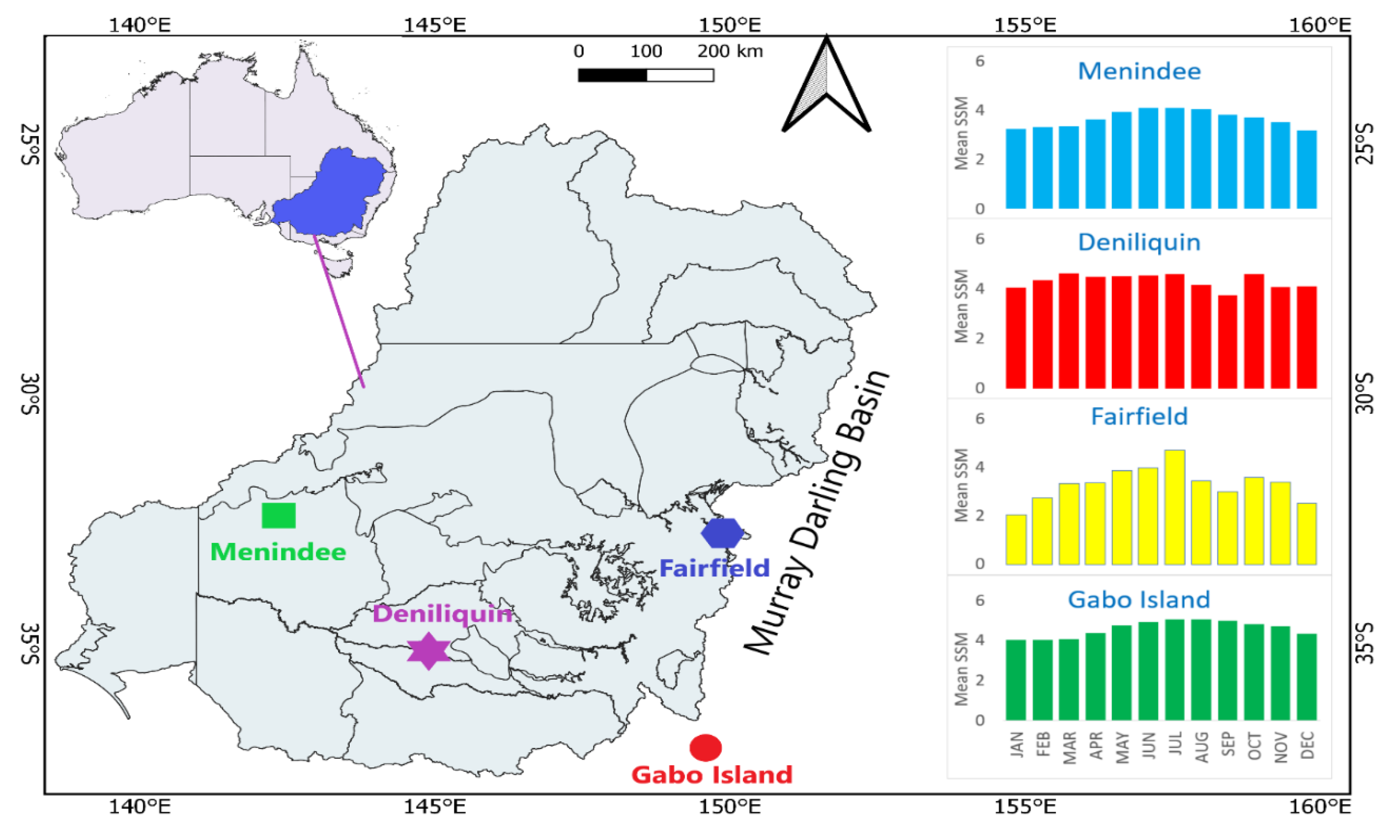
For the first time, this study aims to build a new forecast for daily surface soil moisture (SSM) with convolutional-gated recurrent unit neural networks within the Australian Murray Darling Basin (MDB). The MDB covers ~1,042,730 km2 (or 14%) of mainland Australia [24,66] and ~67% of agricultural lands [67]. As illustrated (Figure 2), the sites are selected based on climate class and soil type diversity, namely Menindee, Deniliquin, Fairfield, and Gabo Island.
The geographical locations and physical characteristics of the sites in Murray Darling Basin are tabulated in Table 1. It should be noted that the site Gabo Island is located at the border of the MDB region for comparison purposes with the other study stations, whereas ~20 lakes surround Menindee in a harsh desert environment. The site Fairfield lies within the savannah climate class with land-use patterns of dryland cropping [23]. Figure 2 also shows a histogram of monthly surface soil moisture patterns for the candidate sites.
The appropriate selection of predictors related to the objective variable has a crucial role in predictive model design. To build a robust model, we adopt remotely sensed MODIS satellite-derived data identified as potential predictor variables in other studies, e.g., solar radiation prediction [24,71,72]. We consider different studies that demonstrate the potential utility of synoptic-scale climate indices that modulate Australian rainfall and crops [41,73,74]. This study integrates three unique data (i.e., satellite-derived data, climate indices, and ground-based variables) to capture a diverse suite of predictive features to forecast SSM, enabling the deep-learning approach a significant edge over the solely station-based models.

3.1.1. MODIS Satellite Dataset

Our hybrid deep learning model (i.e., CEEMDAN-CNN-GRU) is built upon NASA’s Geospatial Online Interactive Visualization and Analysis Infrastructure (GIOVANNI) repository (1 February 2003 to 31 March 2020). GIOVANNI represents a powerful online visualisation and analysis tool for geoscience datasets, capturing 2000 satellite variables [75,76]. In this study, MODIS-based predictor variables, presented in Table 2, are utilised to design and evaluate the hybrid CEEMDAN-CNN-GRU model for SSM forecasting. These are extracted from the GLDAS system representing the high-temporal resolution terrestrial modelling system consisting of the land surface state and several flux parameters with three temporal resolution products: hourly, daily, and monthly. Our study has used GLDAS 2.0 datasets extracted in daily temporal resolutions available publicly. The study utilised MODIS-based surface soil moisture (SSM) data as a target variable obtained from the GLDAS 2.0 model.

3.1.2. Scientific Information for Landowners (SILO) Dataset

To increase the pool of predictors, enabling effective feature engineering and increased performance of the DL model, this study selects nine meteorological variables from Scientific Information for Landowners (SILO): https://www.longpaddock.qld.gov.au/silo/ppd/index.php (accessed on 31 December 2020). SILO, managed by the Department of Environment and Science, Queensland Government [77], is popular for studying the Australian climate. Table 2 provides a list of SILO data.

3.1.3. Climate Indices

In previous studies, e.g., [9,29,59,74] on modelling precipitation, streamflow, and soil moisture, the role of synoptic-scale and climate indices were found significant in improving the overall model. In this study, twenty-one climate indices are thus obtained from many sources: National Climate Prediction Centre, Australian Bureau of Meteorology [70], and National Oceanic and Atmospheric Administration (NOAA) with daily sea surface temperature (Nino1 + 2SST, Nino3SST, Nino3.4SST, Nino4SST) over 1 March 2003 to 31 March 2020 from KNMI Climate Explorer [78]. As the positive SOI is related to La-Nina and negative SOI concurs with El-Nino events [79,80], this study has used all of these indices due to strongly correlated rainfall with lagged SOI showing high predictability of rainfall from August-November [44,81]. To further enhance the predictive skill of the deep learning model, we consider Madden-Julian Oscillation (MJO) known to produce a substantial effect on tropical weather [70], which indeed entails a change in rainfall, wind, sea surface temperature (SST), and cloudiness [82]. Hence, eight daily MJO indices were adopted from KNMI. Climate Explorer [78], together with Interdecadal Pacific Oscillation (IPO), was introduced by Henley et al. [83], collected from NOAA National Climate Prediction Centre. Detailed information on climate indices and SSTs are in Table 2.

3.2. Predictive Model Development

To design a forecast model for SSM over multi-step periods of 1st, 5th, 7th, 14th, 21st, and 30th day lead time, three distinct datasets from satellites (i.e., GIOVANNI), climate indices, and ground source (SILO) for 17 years, 1 February 2003 to 31 March 2020 are used. Hybrid DL is implemented under Intel i7 @ 1.5 GHz and 16 GB memory. The proposed model algorithms were demonstrated using freely available DL libraries, namely the Keras [85,86] and TensorFlow [87] libraries. MATLAB 2020 software is used for Neighbourhood Component Analysis feature selection with packages matplotlib, and Minitab is used to visualise the forecasted SSM in the testing phase.
Data-driven models were built by normalising the input variables, transforming these predictors into a more consistent form [88]. To ensure the variable features were given proportional attention in network training, all were normalised [89] between (0, 1) [41,53,90].
x n o r m = x x m i n x m a x x m i n
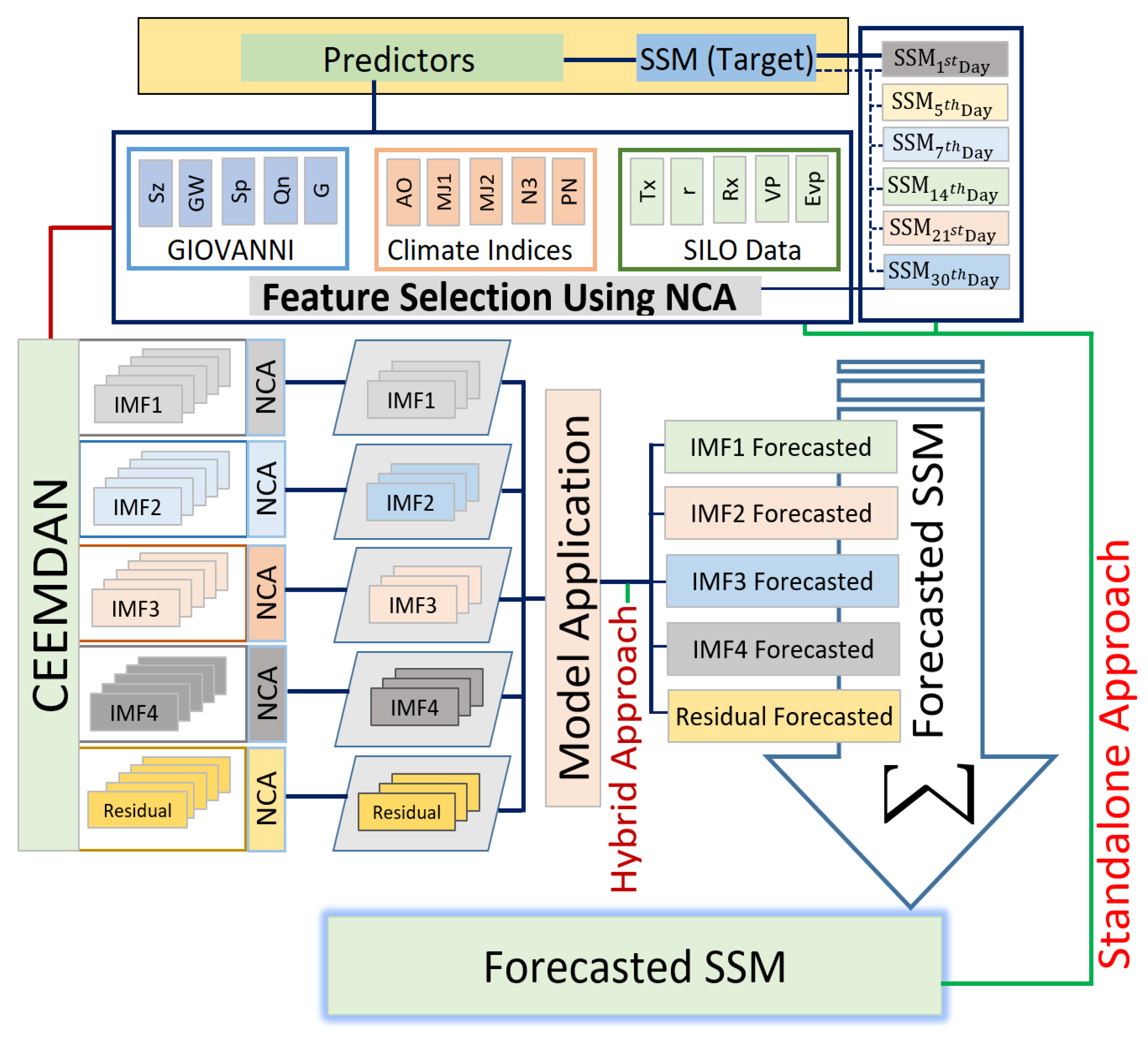
In Equation (15), x is the respective variable, x m i n is the minimum value, x m a x is the maximum and x n o r m is the normalised value. After normalising the variables, the datasets are partitioned into training (February 2003–December 2013), validation (January 2014–December 2016), and testing (January 2017–March 2020) subsets. Figure 3 shows the methodological steps of the proposed CEEMDAN-CNN-GRU model. CEEMDAN is implemented in four stages.

3.2.1. Feature Selection

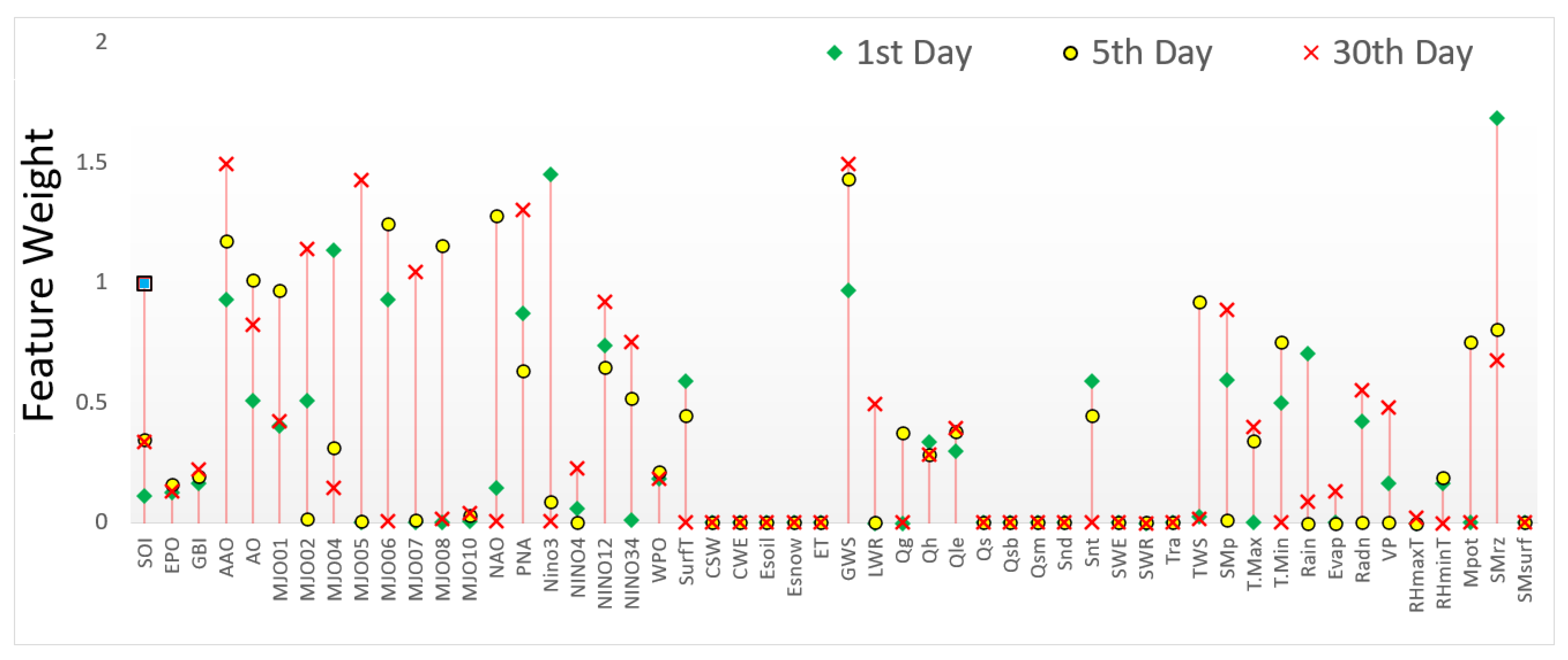
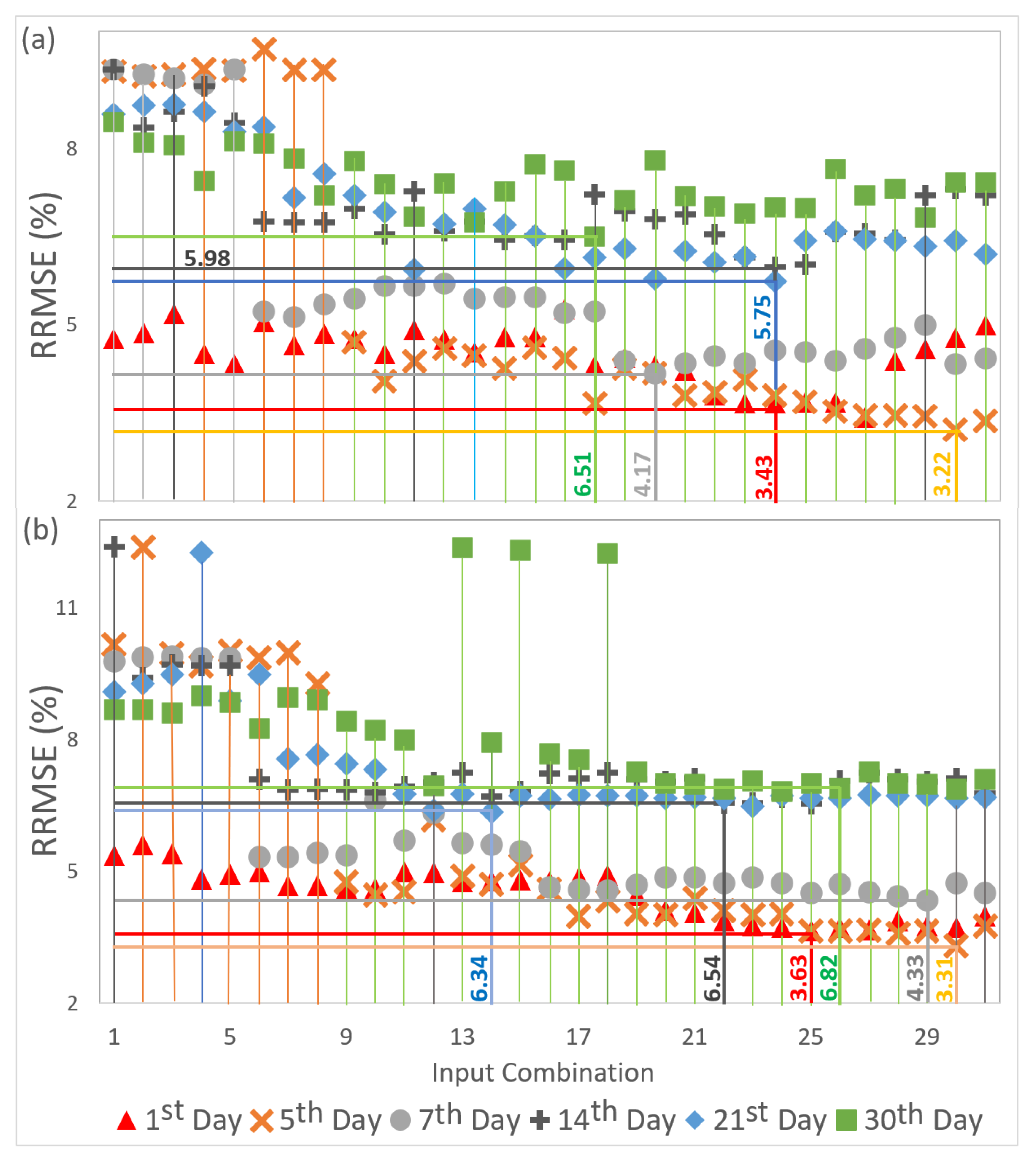
By incorporating the MODIS satellite and ground and climate indices, this study has utilised 52 different predictors for SSM forecasting; hence, feature selection was crucial for data pre-processing. This is because irrelevant and redundant features increase the network size, congestion and cause a reduction in the algorithm’s speed, reducing the efficiency of the predictive model [91]. Therefore, our study has used the NCA algorithm to screen an optimal set of predictor variables out of the 52-variable set. In general, fsrnca calculates every predictor’s relative weight against a target (SSM), illustrated in Figure 4. Following this, the standalone GRU and hybrid CNN-GRU models were executed with predictors added one by one from the highest feature to the lowest feature weight until an optimal performance was achieved. Figure 5 illustrates the the relative root mean squared error (RRMSE) value of different combinations prepared based on NCA. Tables A1–A6 shows the GRU and CNN-GRU model’s performance accordingly.
Figure 4 illustrates the respective feature weights of predictor variables, using the Menindee station as an example. For the 1st day of SSM forecasting, the root zone soil moisture (kg m−2) is found to generate the highest feature weight, whereas, for the 5th day, groundwater storage (mm) is found to be the most significant feature weight. Notably, the groundwater storage contributed to the largest feature weighted for the 7th, 14th, 21st, and 30th day SSM forecasting. This evaluation indicates that groundwater has a strong influence on SSM over inter-daily scales. Tables S1–S6 illustrates the input combination for SSM forecasting in the nth day lead period with their respective forecasting performance with CNN-GRU and GRU model. It is imperative to note that fsrnca algorithm is used in two distinct phases before applying the hybrid-deep learning (i.e., CEEMDAN-CNN-GRU) model. In the first phase, fsrnca attains the feature weights and acquires the optimal predictor variable list required for SSM forecasts. Subsequently, the second phase incorporates the data decomposition process utilising CEEMDAN to each variable selected from the feature weights. Finally, the feature weight is calculated for IMF (t) deduced for each predictor variable against the objective variable (i.e., SSM). Here, the term t refers to the number of IMFs for each variable, removing four to five least significant features from the hybrid CEEMDAN-CNN-GRU model.

3.2.2. Hybrid Deep Learning Algorithm Implementation

Before applying the CEEMDAN-CNN-GRU model in the 1st, 5th, 7th, 14th, 21st, and 30th day SSM forecasts, hyperparameter selection is undertaken through a grid search procedure whose theoretical descriptions are provided in Section 2. Table 3 shows the hyperparameters, optimal GRU architecture, and CNN-GRU with input combinations deduced from the feature weight matrix. Finally, the deep learning forecast model combining a data decomposition (i.e., CEEMDAN) stage with a three-layered feature extraction stage (i.e., CNN) and feature selection stage (i.e., fsrnca) is implemented to forecast SSM.
The proposed CEEMDAN-CNN-GRU model is implemented in four stages, as shown in Figure 3. Firstly, CEEMDAN is applied to decompose historical training data into IMFs and residual signals (Figure 1a) followed by segregation of each IMFs and residual, such as collecting all the IMF1 for predictor variables. The relative feature weights of respective IMFs related to IMF of the target variable (i.e., SSM) are determined. The optimal signal selection enables the algorithm to remove the least important feature-weighted IMFs, allowing the predictive model network to be noise-free. Finally, the forecasted SSM utilising the CEEMDAN-based model (i.e., the hybrid CEEMDAN-CNN-GRU) is obtained by aggregating the IMFs of the predictor variables. The robustness of the model is investigated by several evaluation criteria (Section 3.2.3).
It is worth noting that climate indices (CIs) have a notable signature of climate variability in Australia, leading to substantial influence on rainfall and a potential effect on future surface soil moisture patterns. In the final task, climate indices’ relative contribution to building the CEEMDAN-CNN-GRU model is assessed by Multivariate Adaptive Regression Splines (MARS) utilising the ARESLab toolbox. Following Friedman [86], MARS can determine each predictor variable’s significance by evaluating its complex and non-linear interaction with the target (i.e., SSM) based on best regressors and provide the importance of each variable. The relative importance of any predictor variable is the square root of GCV (Generalised Cross-Validation) with all basic functions involving the respective variable minus the root square of the GCV score of that full model. However, this process is scaled in such a way that the relative importance has a value of 100, expressed:
G C V = M S E ( 1   e n p N ) 2
Here, enp is the significant number of model parameters, p = k + c   ( k 1 ) / 2 ; k = basis function in MARS model; c = penalty (set to 2 or 3). However, if enp is greater or equal to N, GCV is an Inf, which indicates the model is flawed [92].

3.2.3. Predictive Model Evaluation

The efficacy of deep learning hybrid model is evaluated using different performance evaluation criteria e.g., Pearson’s Correlation Coefficient (r), root mean square error (RMSE), Nash-Sutcliffe efficiency (NSE) [93], mean absolute error (MAE), and Kling-Gupta efficiency [94]. Due to geographic differences between the study stations, we employ relative error-based metrics: i.e., relative RMSE (denoted as RRMSE) and relative MAE (denoted as RMAE). The appraisal of a predictive model’s efficacy depends on the exactness between the predicted and observed values. RMSE is an appropriate measure of model performance compared to MAE when the error distribution in the tested data is Gaussian [95] but for an improved model evaluation, the Willmott’s Index (WI) and Legates-McCabe’s (LM) Index are used as more sophisticated and compelling measures [96,97]. Mathematically, the metrics are as follows:
Correlation coefficient (r):
r =   { i = 1 N ( S S M o b s S S M ¯ o b s ) ( S S M f o r S S M ¯ f o r ) i = 1 N ( S S M o b s S S M ¯ o b s ) 2   i   = 1 N ( S S M f o r S S M ¯ f o r ) 2 } 2
Mean absolute error (MAE: kg m−2):
M A E = 1 N i = 1 N | S S M f o r S S M o b s |  
Root mean squared error (RMSE: kg m−2):
R M S E = 1 N i = 1 N ( S S M f o r   S S M o b s ) 2
Nash-Sutcliffe Efficiency (NSE):
N S E = 1   [ 1   i = 1 N ( S S M f o r ) 2 i = 1 N ( S S M o b s   S S M ¯ f o r ) 2 ] )
Kling-Gupta efficiency (KGE):
K G E = 1   ( r 1 ) 2 + ( S S M ¯ f o r S S M ¯ o b s 1 ) 2 + ( C V p C V s ) 2
Mean Absolute Percentage Error (MAPE, %):
M A P E = 1 N   ( N t = 1 |   ( S S M f o r     S S M o b s ) S S M o b s   | ) × 100 ,   ( 0 % M A P E 100 % )
Willmott’s Index (WI):
W I   =   1   [ i = 1 N ( S S M f o r S S M o b s ) 2 i = 1 N ( | S S M f o r S S M ¯ o b s | +   | S S M o b s S S M ¯ o b s |     ) 2 ]
Legates–McCabe’s Index (LM):
L M   =   1   [ i = 1 N | S S M f o r S S M o b s | i = 1 N | | S S M o b s S S M ¯ o b s | | ]
Relative Root Mean Squared Error (RRMSE, %):
R R M S E ( % ) =   1 N i = 1 N ( S S M f o r S S M o b s ) 2 1 N i = 1 N ( S S M o b s )   ×   100
Relative Mean Absolute Error (RMAE, %):
R M A E   ( % ) =   1 N i = 1 N | S S M f o r S S M o b s | 1 N i = 1 N ( S S M o b s )   ×   100
Absolute percentage bias (APB, %):
A P B   =   [ i = 1 N | S S M o b s S S M f o r |   ×   100 i = 1 N | S S M o b s | ]
In Equations (17)–(27), S S M o b s and S S M f o r represents the observed and forecasted values for ith test value; S S M ¯ o b s and S S M ¯ f o r refer to their averages, accordingly, and N is defined as the number of observations, while CV stands for the coefficient of variation. CV is a standardised measure of the dispersion of the frequency distribution.

4. Results

The practical utility of the hybrid DL (i.e., CEEMDAN-CNN-GRU) model is established by integrating diverse data in its training and model testing phase. Significant features from predictor variables are used by incorporating NCA, and the predictive model is evaluated using statistical metrics (Equations (17)–(27)), infographics, and visualisations to appraise the degree of agreements between simulated and observed soil moisture. By several measures, the CEEMDAN-CNN-GRU model appears to outperform all the comparative models with superior r and NSE and low RMSE, MAE, and APB in the testing phase. An extensive analysis of tabulated results (Table 4) provides convincing arguments that the hybrid deep learning method is effective for surface soil moisture forecasts and can perhaps be a potential tool in agriculture water management. However, among all study sites, the CEEMDAN-CNN-GRU model for the Menindee station showed the best performance, considering r (0.996), NSE (0.995), and lowest RMSE (0.021), MAE (0.013), and APB (0.359) values for the 1st day of SSM forecasting. The performance of this model is followed by the CEEMDAN-GRU and CNN-GRU model.
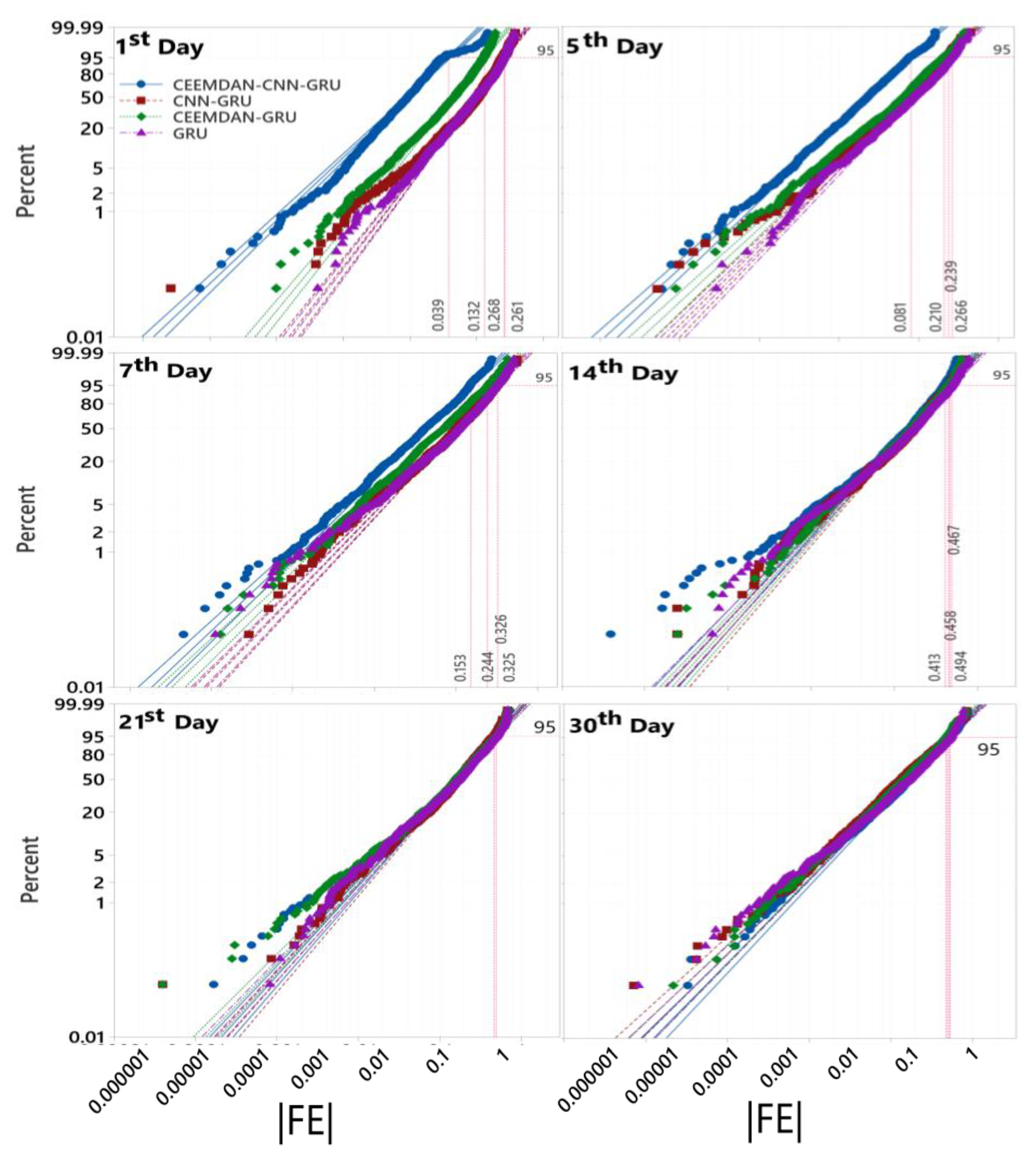
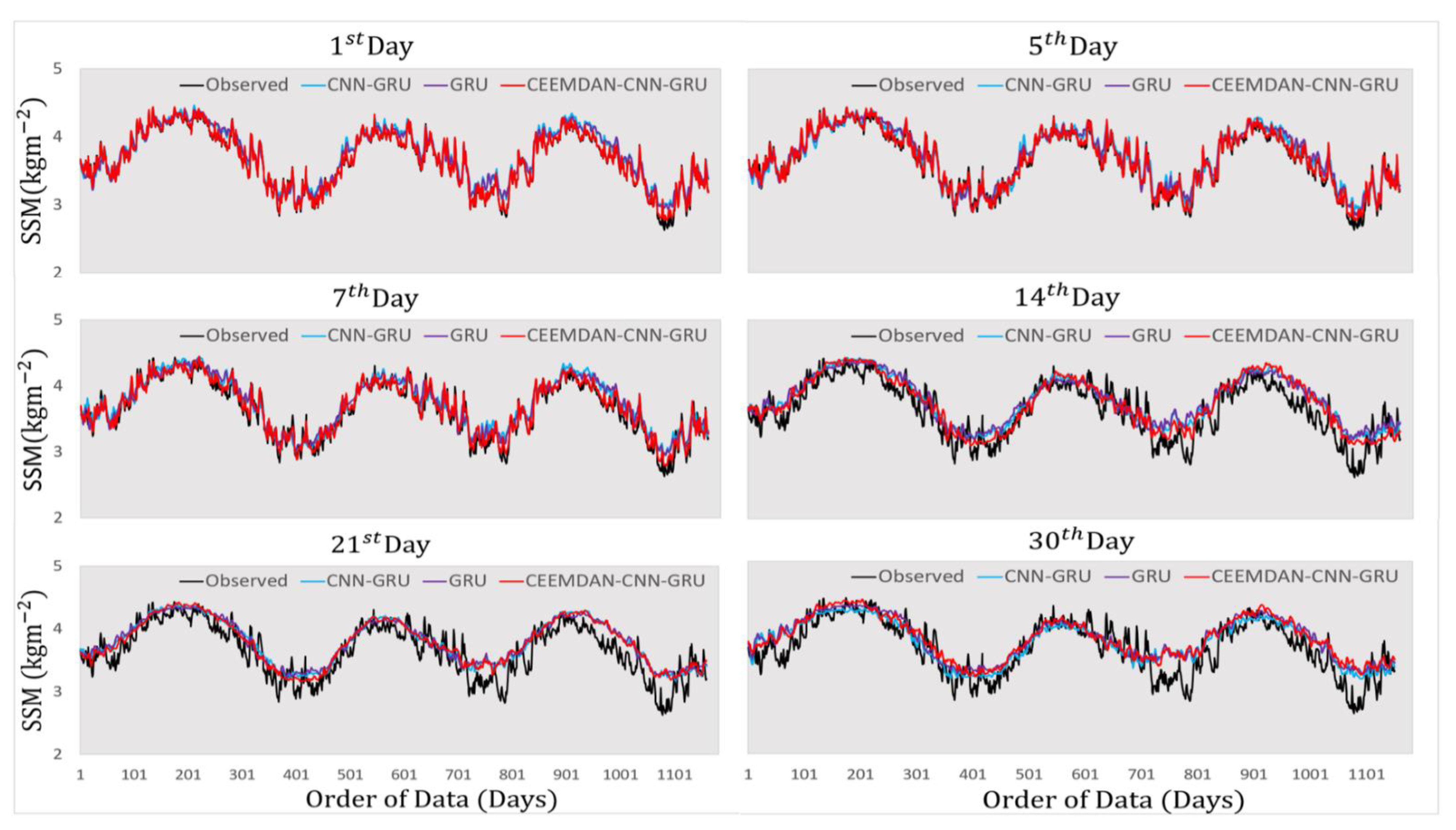
For the 5th day of SSM forecasting, the results of the objective model for Menindee had the best performance (r = 0.993; NSE = 0.991; RMSE = 0.040 kg m−2) followed by Deniliquin (r = 0.989; NSE = 0.975; RMSE = 0.091 kg m−2). Likewise, for the 7th, 14th, 21st, and 30th days of SSM forecasting, the CEEMDAN-CNN-GRU model outperformed the other models by a notable margin for all the respective periods of SSM forecasting. However, a site-specific signature in the model accuracy was also evident, with the results for Menindee registering the lowest value of RMSE generated by the CEEMDAN-CNN-GRU model. In terms of MAE, the CEEMDAN-CNN-GRU model returned the lowest value for Menindee, suggesting that the CEEMDAN-CNN-GRU model was a potential forecasting tool SSM at the 1st, 5th, and 7th day ahead periods. Not surprisingly, in accordance with other studies, e.g., the present study indicates that as the length of the forecasting period was increased, the model’s performance appear to reduce at a significant rate in such a way that the r-values reduced by 0.30%, 1.10%, 9.15%, 11% and 15% for the 1st to 5th, 7th, 14th, 21st and 30th day of SSM forecasting. The change of the performance metrics (i.e., NSE, MAE, and APB) for longer-term horizons relative to the shorter-term horizons also concurred with the respective changes in the r-values and is consistent with earlier studies [60,98]. For a longer-term horizon, the present r value was lower, and the MAE increased, suggesting that for the longer forecast horizon, the model appeared to lose the relevant data features in the predictor variables required to maintain precise SSM forecasting performance. The hybrid CEEMDAN-CNN-GRU model is further evaluated using a probability plot of errors at the 95th percentile, including those of the benchmark model (i.e., CNN-GRU, CEEMDAN-GRU) and the standalone model (i.e., GRU) with an illustration for Menindee at the different nth (n = 1, 5, 7, 14, 21 and 30) days (Figure 6). The CEEMDAN-CNN-GRU model results show that ~95% of SSM forecasting had the lowest error (<0.1) for the 1st and 5th days of SSM forecasting. Among all the predictive models and the forecast periods over nth days, the GRU-based model showed a more significant proportion of |FE| values at a 95% confidence level. Notably, consistently good results were also achieved for the other stations (i.e., Deniliquin, Fairfield, and Gabo Island), which are shown in supplementary materials (Figure S1a–c). The lowest value of |FE|, with <0.063 with a 95% percentile, was evident for Fairfield compared to the other two study stations. The correlation between observed and forecasted daily surface soil moisture datasets generated by the proposed CEEMDAN-CNN-GRU model vs. the corresponding benchmark models (i.e., CNN-GRU and GRU), for the case of Menindee station, is illustrated in Figure 7. The correlations for the hybrid GRU model are positioned close to the observed SSM values up to the 7th day, revealing a high degree of forecasting accuracy. An improvement in the model’s forecasting performance was attained by applying the CNN algorithm (i.e., soil moisture generated by the CNN-GRU model) and data decomposition (i.e., CEEMDAN-CNN-GRU) method on standalone GRU model. The disparity between the forecasted SSM and the reference SSM values was significantly higher for the 14th, 21st, and 30th days of SSM forecasting, which concurs with earlier metrics suggesting a potential inadequacy of the data features long time ahead periods [60].
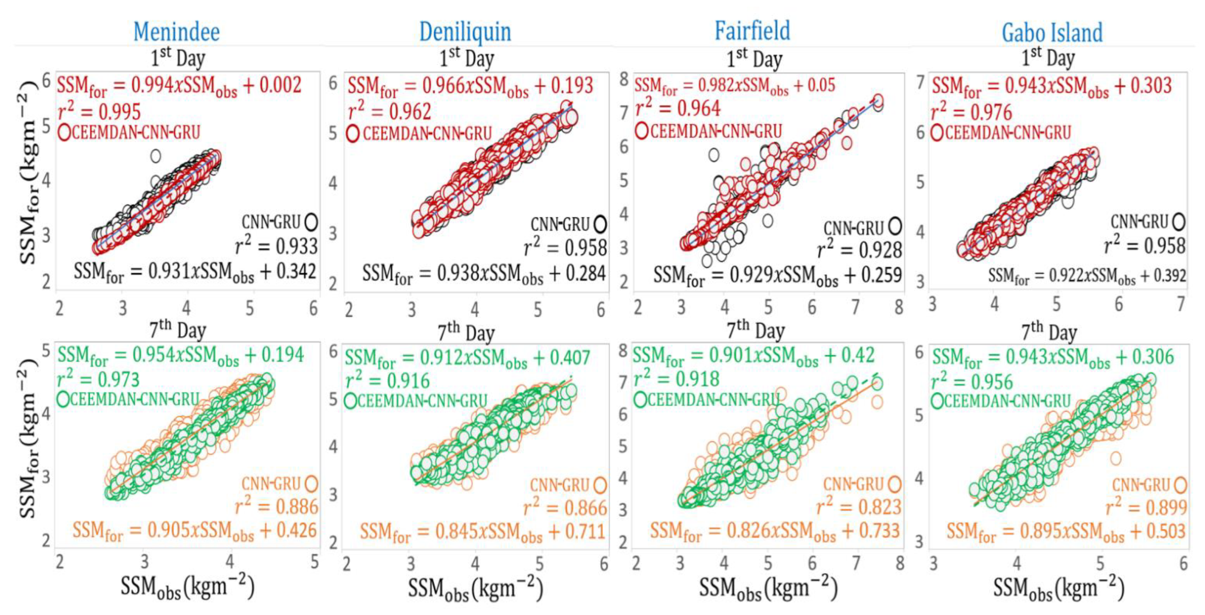
Figure 8 shows a scatter plot of forecasted and observed SSM for the 1st and 7th days across the Murray Darling Basin with a least square regression line, y = mx + C, and the coefficient of determination in each sub-panel. Notably, the objective model (i.e., CEEMDAN-CNN-GRU) is seen to attain more accurate results with considerably larger r2 values. The SSM forecast with a hybrid deep learning model for Menindee station performed significantly better than the comparative model (i.e., CNN-GRU). In the case of Menindee, for example, the values for m and r2 are in reasonably good agreement against the 1:1 line representing the forecasted and observed SSM values in such a way that (m|r2) is 0.994|0.995 for the hybrid CEEMDAN-CNN-GRU model relative to (0.931|0.933) for CNN-GRU for the 1st day ahead of SSM forecasting. Moreover, for the 1st day of SSM forecasting, the CEEMDAN-CNN-GRU model provided results in significant proximity to the other three stations, such as Deniliquin: 0.962|0.966, Fairfield: 0.928|0.964, and the Gabo Island: 0.958|0.976). Alternatively, the y-intercept of the regression line was close to trivial, i.e., 0.002 (Menindee: 1st day), 0.193 (Deniliquin: 1st day), 0.05 (Fairfield:1st day), and 0.303 (Gabo Island:1st day), revealing the efficacy of the deep learning hybrid method for surface soil moisture forecasting. For the 14th, 21st, and 30th day ahead of SSM forecasting, the y-intercept, as expected, deviated slightly from the ideal value of 0, caused by more outliers between simulated and reference values in the testing phase.
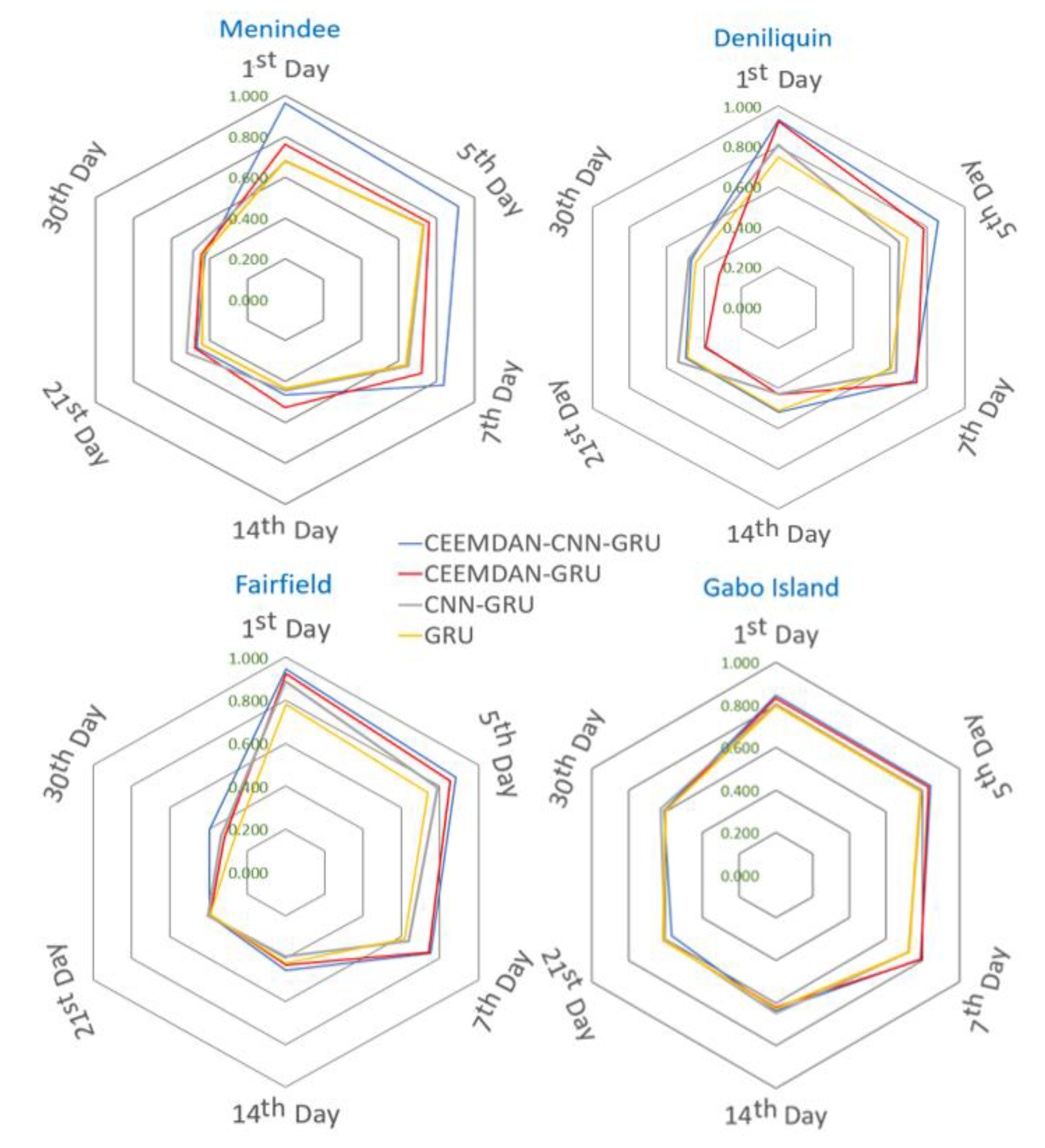
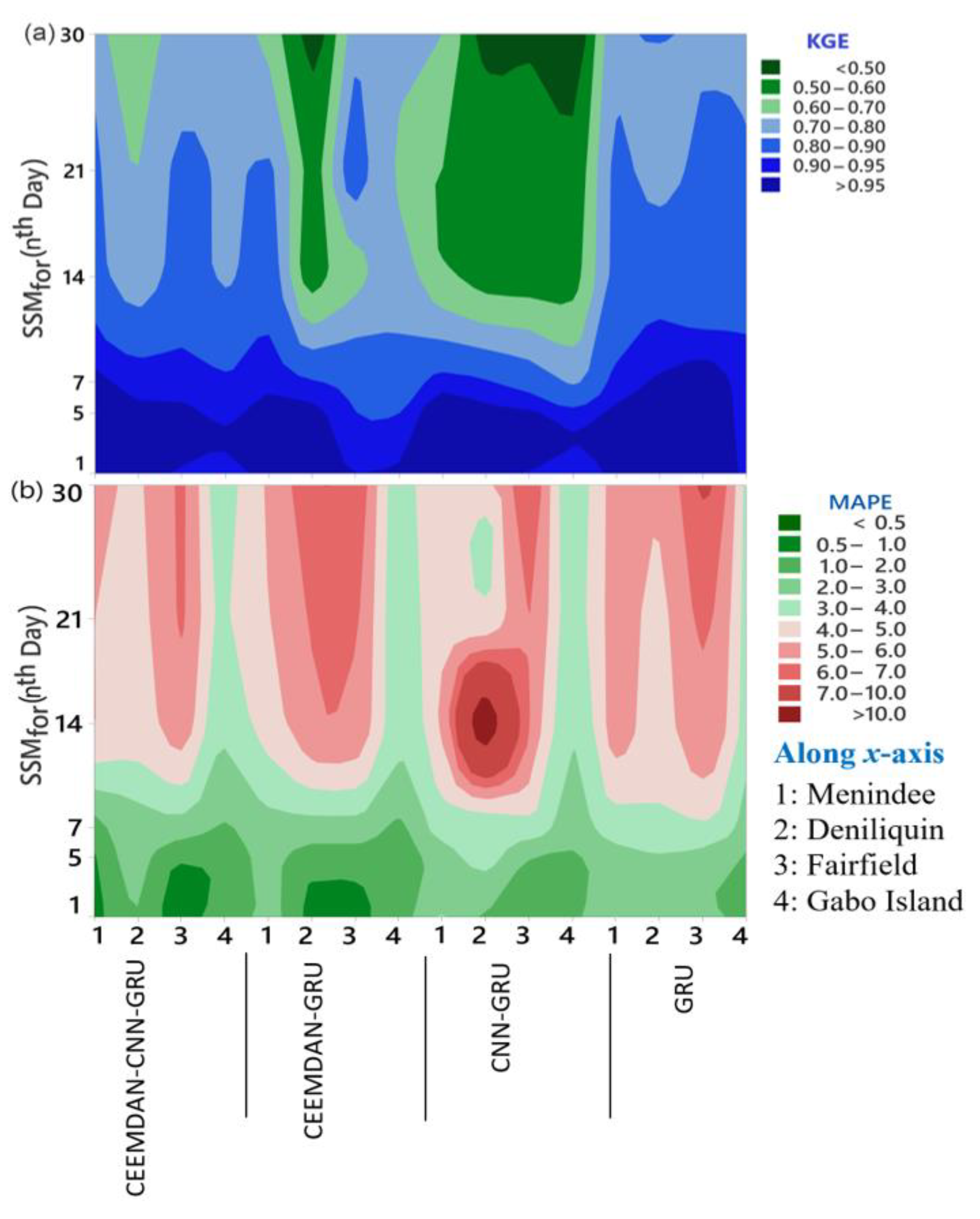
To further analyse the tested models’ performances, we adopt the Legates and McCabe’s Index [99] as a cross-validation metric for simulated data. This metric has a better model penalisation skill when high SSM values are expected in the testing set [41]. This is illustrated in Figure 9 in terms of a polar plot of the LM values for the hybrid deep learning approach (i.e., CEEMDAN-CNN-GRU) and other models for the different day ahead forecasting. The LM values accumulated across all stations in the case of CEEMDAN-CNN-GRU have a superior result with the highest LM ≈ 0.962 for Menindee and the lowest LM for the case of Gabo Island (LM ≈ 0.846) in the 1st Day ahead SSM forecasting. In agreement with earlier results, the LM values for the 14th, 21st, and 30th day ahead for other models were comparatively smaller. Figure 10a,b is a contour plot of KGE and MAPE for the hybrid DL approach (i.e., CEEMDAN-CNN-GRU) along with its benchmark (i.e., CNN-GRU) and standalone (i.e., GRU) methods for all four stations in MDB at different nth (n = 1, 5, 7, 14, 21 and 30) days in forecasting SSM. This infographic verifies the robustness of the proposed objective model that attains the highest KGE values and the lowest MAPE values for 1st and 5th day of SSM forecasting.
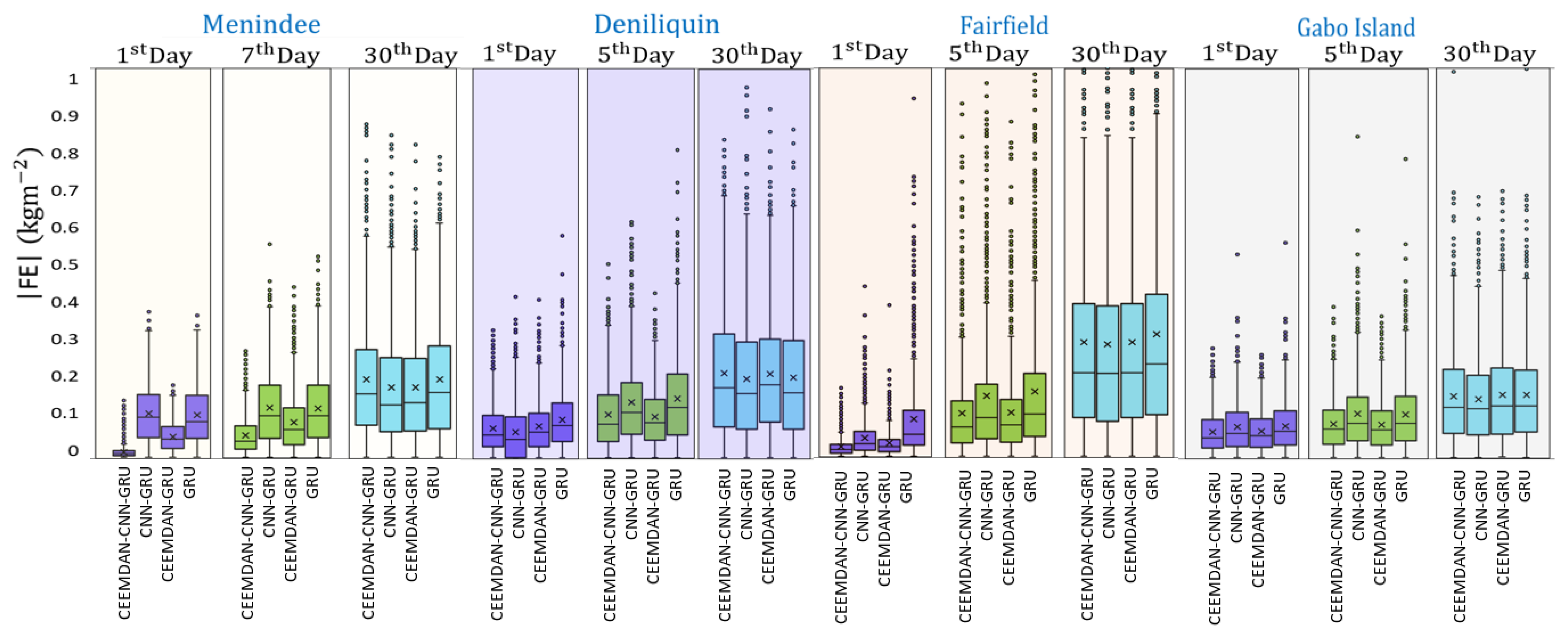
However, for the 14th, 21st, and 30th day of SSM forecasting, the KGE values range between 0.40 and 0.80, and the MAPE values range from 4–11%, demonstrating a slightly lower forecast accuracy relative to the 1st and 5th day of SSM forecasting. Figure 11 illustrates the absolute forecasted error (|FE|) using all the four candidate study sites’ implemented models. The box plot demonstrates the data dispersal in terms of the forecasted (SSMfor) SSM. Figure 11 provides a clear visualisation of the closed distribution of error values for Menindee and Fairfield stations in the hybrid CEEMDAN-CNN-GRU model for 1st day ahead SSM forecasting. The lower end of the plot for |FE| is situated within the lower quartile (25th) and upper quartile (75th). Moreover, the GRU and CNN-GRU models for these stations show an increased distribution of |FE|, except for the Fairfield station. Moreover, the forecasting of SSM for the 14th, 21st, and 30th day periods have a comparatively higher value of the absolute forecasting error for all tested models. A more comprehensive inspection of the absolute forecasting error (|FE|) in the case of the hybrid GRU. model for the four study stations further cements the suitability of the CEEMDAN-CNN-GRU model in forecasting SSM for the 1st, 5th, and 7th day ahead periods in Australian Murray Darling Basin, evidenced by the narrowest error distribution in comparison with the other models.
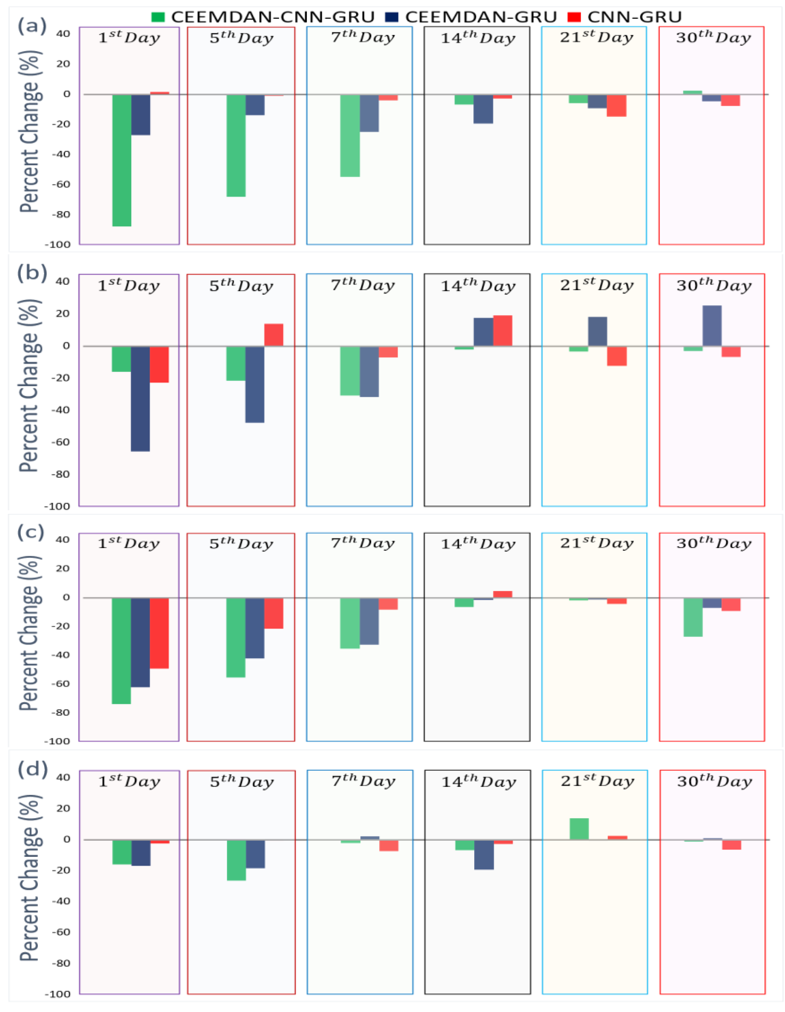
It is noteworthy that in this study, two distinct algorithms, namely the CEEMDAN and CNN, are used to improve the GRU-based predictive model. Therefore Figure 12 shows the effect of applying CEEMDAN and CNN as data pre-processing and feature extraction methods incrementally, respectively, on the per cent change in RMAE values within the testing SSM values. In terms of 1st, 5th, and 7th day of Menindee station, the RMAE (%) values of CEEMDAN-CNN-GRU model (where both CEEMDAN and CNN are integrated) appeared to decrease by ~87%, 68%, and 54%, respectively. Similarly, for the 1st-day forecasting taking the example of Fairfield station, the CNN feature-extraction skill reduced the error of ~55%, whereas an additional decrease in RMAE of ~18% was noted integration of the CEEMDAN selected variables (CEEMDAN-CNN-GRU). Additionally, for Deniliquin and Gabo Island study sites, the SSM forecasting for the 1st day ahead evaluated through RMAE values decreased by slightly less than 20%. It is worth mentioning that the per cent increase in RMAE was ~5% for Menindee for the 30th day ahead SSM forecasting with similar deductions for the other stations.
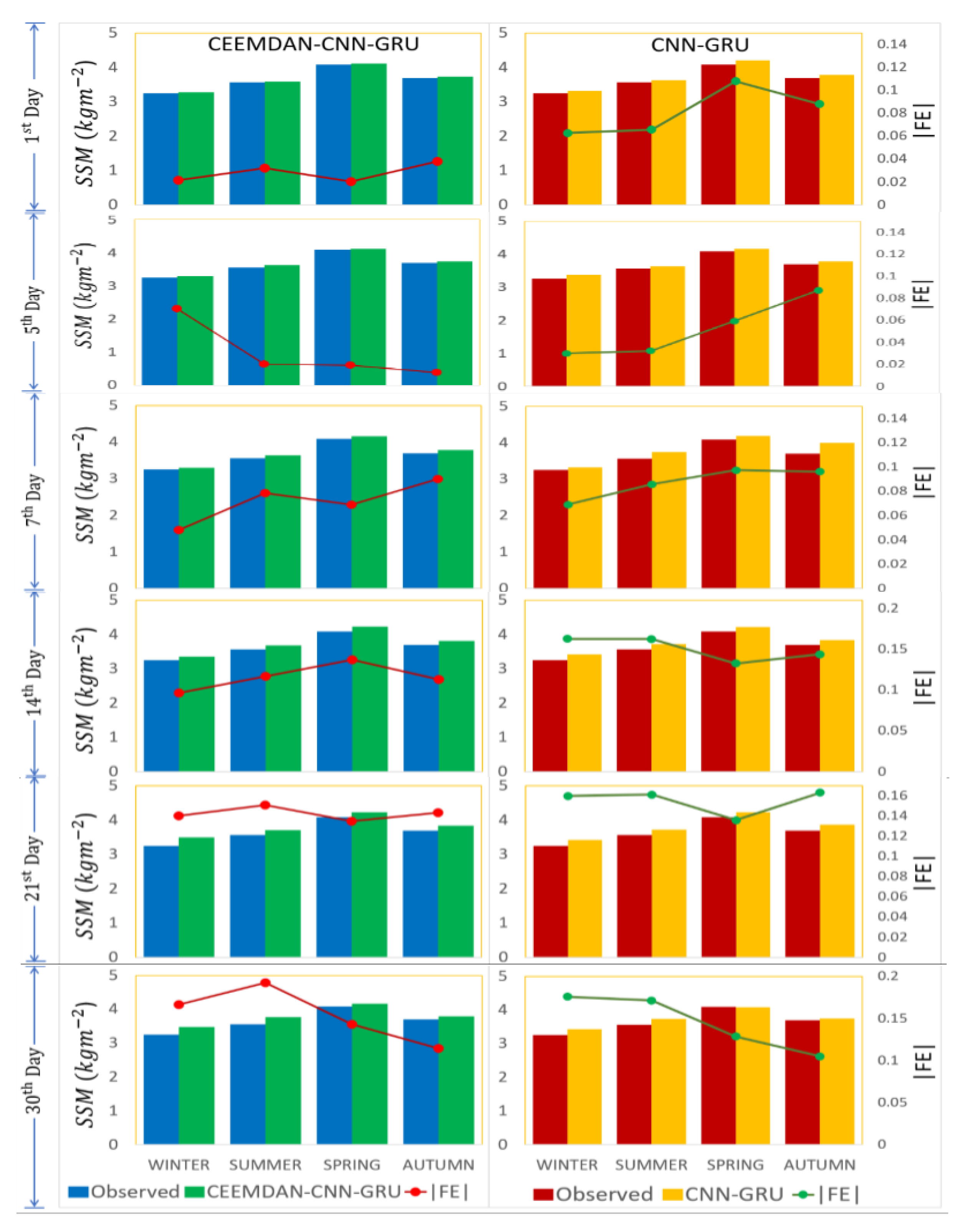
We further show the CEEMDAN-CNN-GRU hybrid model’s skill for seasonal forecasting for the different day ahead periods to better understand the seasonal effects of models used in SSM prediction. Figure 13 displays the average observed vs forecasted SSM on a seasonal basis (i.e., austral summer, autumn, winter, and spring) generated by CEEMDAN-CNN-GRU model in case of Menindee study site. The forecast error across these seasons is relatively insignificant, occupying values of (0, 0.16) kg m−2 to demonstrate the exceptional skill of the objective model. Notably, the 1st and 5th day ahead of observed and forecasted SSM for austral summer, spring, winter, and autumn appear to match with the forecast error (|FE|) < 0.04 kg m−2, whereas, for winter, the |FE| values are slightly higher for the 5th day ahead SSM forecasting. Not surprisingly, the CNN-GRU model possesses a larger error, ranging from 0.04 to 0.18 kg m−2, establishing the CNN-GRU model’s relatively poor performance compared with the hybrid CEEMDAN-CNN-GRU model. For the case of the 30th day ahead SSM forecasting, the study site Menindee registered a higher uncertainty for austral summer (0.18<|FE|< 0.18 kg m−2) compared with winter and spring (0.14 < FE < 0.15 kg m−2). This indicates that the hybrid CEEMDAN-CNN-GRU model developed with NCA and CEEMDAN algorithms employing MODIS-derived satellite data, ground-based observations, and climate indices can be considered ideal in multi-step SSM forecasting.

5. Discussions

Based on the results, we note the effects of climate indices on surface soil moisture as non-negligible. In this paper, analysing this impact is undertaken using two ways. Firstly, the NCA algorithm provides key information about how climate indices affect SSM. For example, for SSM forecasting, climate indices based on SOI, EPO, MJOs and SST were found to significantly affect the SSM. Secondly, GCV values based on a MARS model were calculated following Friedman [100] approach to deduce the importance of input features. The contributory influence appeared to be between 12% and 53% according to GCV for Menindee station, and similarly notable effect for the other study sites. Specifically, the lowest percentage of ~12% of GCV was found for the 14th, and the highest percentage (~53%) was found for the 28th Day ahead SMM forecasting. In a nutshell, we note that climate indices make a moderate to high contribution in forecasting surface soil moisture within the Murray Darling Basin.
Neighbourhood Component Analysis (NCA) was utilised to examine significant features from a relatively large pool (or 52 different) data related to soil moisture. In data-driven modelling, selecting predictor variables is crucial, as improper variables with weak relationships against SSM can lead to undesirable uncertainties in the model. As per evaluations in Tables S1–S6, a combination of predictor variables deduced by NCA at six different lead time SSM forecasting was significant, and this result concurred with previous studies [59,101].
The objective approach based on NCA yielded good accuracy (i.e., CEEMDAN-CNN-GRU), demonstrating that best predictors were attained through a careful variable selection stage (by NCA) and feature extraction stage (by CNN and CEEMDAN methods). Accordingly, the proposed forecast model for SSM was sufficiently robust in daily and seasonal tests, as well as through the inclusion of synoptic-scale features, i.e., those captured from patterns in the SST and MJO series. The probability of absolute error placing within the 95th percentile and the substantial seasonal forecasting of SSM indicates that the model can handle satellite-derived variables’ error. Our study also suggests that groundwater recharge, deep percolation, and plant uptake, which are essential factors to concentrate soil moisture in different layers [57], can be ideal variables to better understand SSM characteristics while also assisting in the prediction of future changes.
The present model’s performance revealed that a shorter period forecast (i.e., 1st, 5th, or 7th) was more precise, whereas a longer forecast horizon (i.e., 14th, 21st, and 30th) registered a lower accuracy than that of the shorter span of SSM forecasting. One plausible reason for this is that our predictive model appeared to struggle to capture enough input features from the dataset for a more extended time-step forecast (i.e., 30th day against 7th day). Considering the reduction in feature capturing capability of the model, we can say that as the time series data approached close to the 7th-day boundary, the model would capture it with good forecast accuracy. Undoubtedly, this occurs due to a loss of data features in the predictor-target matrix. This indeed concurs with earlier studies (e.g., [60,98], where models for the 1- and 2-day ahead modelling horizon was more accurate than the 30-day horizon for river flow forecasting, and the 1- and 3-month runoff model was more accurate than the 6-month runoff model predicting 1-, 3-, and 6-month ahead runoff in the Yingluoxia watershed, Northwestern China. The hybrid deep learning approach (i.e., CEEMDAN-CNN-GRU) incorporated with MODIS satellite-derived data, ground-based SILO data, and climate mode indices (representing synoptic-scale climate features) can be a good modelling tool to predict soil moisture or other hydrological variables at multi-step lead times, including its future use in water resource management and sustainable agriculture.

6. Conclusions

This study reports the performance efficacy of a DL data-driven (CEEMDAN-CNN-GRU) model based on the Gated Recurrent Unit (GRU) for daily surface soil moisture forecasting at multi-step horizons. The hybrid CEEMDAN-CNN-GRU model was built by integrating MODIS sensors (satellite-derived data), ground-based observations, and climate indices tested at important stations in the Australian Murray Darling Basin. To attain an accurate and reliable model for soil moisture, a feature extraction (i.e., CNN) and feature (or variable) selection algorithm (i.e., NCA) was used, with tests at 1st, 5th, 7th, 14th, 21st, and 30th day ahead period. The input variables, comprised initially of 52 different predictors, were extracted from March 2003 to March 2020 and screened accordingly, using the NCA algorithm through a feature selection stage, to select the most relevant input variables required to forecast daily-scale soil moisture. Three other benchmarking models (i.e., CEEMDAN-GRU, CNN-GRU, and GRU) were built and evaluated against statistical score metrics and visual analysis to ascertain the predictive skill of the objective model of observed and forecasted datasets in the testing phase. The results revealed that NCA was a practical approach to acquire the best features from an optimal set of predictor variables. The hybrid CEEMDAN-CNN-GRU model has significantly improved the decomposition of input variables to provide more defined soil moisture prediction features. Thus, the proposed CEEMDAN-CNN-GRU model yielded an acceptable level of accuracy when applied at the 1st, 5th, and 7th day ahead SSM forecasting against standalone GRU model registering a comparatively higher forecast error at all these periods. This superior performance was also endorsed with low MAE values, ranging from 0.013 kg m−2 to 0.067 kg m−2, 0.030 kg m−2 to 0.075 kg m−2, and 0.057 kg m−2 to 0.113 kg m−2 for the 1st, 5th, and 7th day ahead period. Other results also supported the practical utility of the CEEMDAN-CNN-GRU model. For example, the probability plot of absolute error for Menindee station has 95% of SSM forecasting with the lowest error bracket (<0.1) at the 1st, and 5th day SSM prediction, and these results were better than earlier studies on forecasting soil moisture prediction, e.g., [23,36,59,102]. As the present study has focused on daily scale prediction, in a future study, researchers may also adopt the CEEMDAN-CNN-GRU model to utilise the global climate model (GCM) model-simulated variables to estimate future SSM under global warming scenarios.

Supplementary Materials

The following are available online at https://www.mdpi.com/2072-4292/13/4/554/s1, Table S1: Performance of CNN-GRU and GRU model to forecast the 1st day Surface Soil moisture of Minendee Station with the optimum forecasting results based on the Nash-Sutcliffe coefficient (NS) and mean absolute error (MAE; Kg m−2) for the testing phase, Table S2: Caption identical to Table S1, except for the 5th day. Table S3: Caption identical to Table S1, except for the 7th day, Table S4: Caption identical to Table S1, except for the 14th day, Table S5: Caption identical to Table S1, except for the 21st day, Table S6: Caption identical to Table S1, except for the 30th day, Figure S1: Probability plot for the objective model (i.e., CEEMDAN-CNN-GRU), benchmark model (i.e., CNN-GRU, CEEMDAN-GRU), and the standalone model (i.e., GRU) for (a) Deniliquin, (b) Fairfield and (c) Gabo Island stations at different nth (n = 1, 5, 7, 14, 21, and 30) days. The reference points are provided at 95 percentiles on the probability of comparing the model.

Author Contributions

Conceptualisation, A.A.M.A. and R.C.D.; methodology, A.A.M.A. and R.C.D.; software, A.A.M.A.; model development, A.A.M.A.; validation, A.A.M.A.; formal analysis, A.A.M.A.; investigation, A.A.M.A.; resources, A.A.M.A.; data curation, A.A.M.A.; writing—original draft preparation, A.A.M.A.; writing—review and editing, A.A.M.A., R.C.D., N.R., A.G., Q.F., Z.Y. and L.Y.; visualisation, A.A.M.A.; supervision, R.C.D.; funding acquisition, R.C.D. All authors have read and agreed to the published version of the manuscript.

Funding

The study was supported by the Chinese Academy of Science (CAS), and University of Southern Queensland (USQ) under the USQ-CAS Postgraduate Research Scholarship (2019–2021) awarded to the first author, managed by Graduate Research School under the leadership of Professor Feng Qi (CAS) and Associate Professor Ravinesh Deo (USQ).

Institutional Review Board Statement

Not applicable.

Informed Consent Statement

Not applicable.

Data Availability Statement

Publicly available datasets were analysed in this study. The data can be found here: [https://giovanni.gsfc.nasa.gov/giovanni/; https://www.longpaddock.qld.gov.au/silo/].

Acknowledgments

We thank the Editor and Reviewers for their insightful comments.

Conflicts of Interest

The authors declare no conflict of interest.

References

  1. Van Loon, A.F.; Laaha, G. Hydrological drought severity explained by climate and catchment characteristics. J. Hydrol. 2015, 526, 3–14. [Google Scholar] [CrossRef] [Green Version]
  2. Brocca, L.; Melone, F.; Moramarco, T.; Morbidelli, R. Spatial—temporal variability of soil moisture and its estimation across scales. Water Resour. Res. 2010, 46, W02516. [Google Scholar] [CrossRef]
  3. Brocca, L.; Ciabatta, L.; Massari, C.; Camici, S.; Tarpanelli, A. Soil Moisture for Hydrological Applications: Open Questions and New Opportunities. Water 2017, 9, 140. [Google Scholar] [CrossRef]
  4. Chang, X.; Zhao, W.; Zeng, F. Crop evapotranspiration-based irrigation management during the growing season in the arid region of northwestern China. Environ. Monit. Assess. 2015, 187, 699. [Google Scholar] [CrossRef]
  5. Gill, M.K.; Asefa, T.; Kemblowski, M.W.; McKee, M. Soil moisture prediction using support vector machines 1. JAWRA J. Am. Water Resour. Assoc. 2006, 42, 1033–1046. [Google Scholar] [CrossRef]
  6. Akbari Asanjan, A.; Yang, T.; Hsu, K.; Sorooshian, S.; Lin, J.; Peng, Q. Short-Term Precipitation Forecast Based on the PERSIANN System and LSTM Recurrent Neural Networks. J. Geophys. Res. Atmos. 2018, 123. [Google Scholar] [CrossRef]
  7. Tripathi, S.; Srinivas, V.V.; Nanjundiah, R.S. Downscaling of precipitation for climate change scenarios: A support vector machine approach. J. Hydrol. 2006, 330, 621–640. [Google Scholar] [CrossRef]
  8. Yang, L.; Feng, Q.; Yin, Z.; Wen, X.; Deo, R.C.; Si, J.; Li, C. Application of multivariate recursive nesting bias correction, multiscale wavelet entropy and AI-based models to improve future precipitation projection in upstream of the Heihe River, Northwest China. Theor. Appl. Climatol. 2018, 137, 323–339. [Google Scholar] [CrossRef]
  9. Nguyen-Huy, T.; Deo, R.C.; An-Vo, D.-A.; Mushtaq, S.; Khan, S. Copula-statistical precipitation forecasting model in Australia’s agro-ecological zones. Agric. Water Manag. 2017, 191, 153–172. [Google Scholar] [CrossRef]
  10. Deo, R.C.; Şahin, M. Application of the extreme learning machine algorithm for the prediction of monthly Effective Drought Index in eastern Australia. Atmos. Res. 2015, 153, 512–525. [Google Scholar] [CrossRef] [Green Version]
  11. Prasad, R.; Deo, R.C.; Li, Y.; Maraseni, T. Input selection and performance optimisation of ANN-based streamflow forecasts in the drought-prone Murray Darling Basin region using IIS and MODWT algorithm. Atmos. Res. 2017, 197, 42–63. [Google Scholar] [CrossRef]
  12. Ahmed, A.M.; Shah, S.M.A. Application of artificial neural networks to predict peak flow of Surma River in Sylhet Zone of Bangladesh. Int. J. Water 2017, 11, 363–375. [Google Scholar] [CrossRef]
  13. Hu, C.; Wu, Q.; Li, H.; Jian, S.; Li, N.; Lou, Z. Deep Learning with a Long Short-Term Memory Networks Approach for Rainfall-Runoff Simulation. Water 2018, 10, 1543. [Google Scholar] [CrossRef] [Green Version]
  14. Kratzert, F.; Klotz, D.; Brenner, C.; Schulz, K.; Herrnegger, M. Rainfall–runoff modelling using Long Short-Term Memory (LSTM) networks. Hydrol. Earth Syst. Sci. 2018, 22, 6005–6022. [Google Scholar] [CrossRef] [Green Version]
  15. Arto, I.; Garcia-Muros, X.; Cazcarro, I.; Gonzalez-Eguino, M.; Markandya, A.; Hazra, S. The socioeconomic future of deltas in a changing environment. Sci. Total Environ. 2019, 648, 1284–1296. [Google Scholar] [CrossRef] [PubMed]
  16. Le, H.; Lee, J. Application of Long Short-Term Memory (LSTM) Neural Network for Flood Forecasting. Water 2019, 11, 1387. [Google Scholar] [CrossRef] [Green Version]
  17. Ahmed, A.M.; Deo, R.C.; Ghahramani, A.; Raj, N.; Feng, Q.; Yin, Z.; Yang, L. LSTM integrated with Boruta-random forest optimiser for soil moisture estimation under RCP4. 5 and RCP8. 5 global warming scenarios. Stoch. Environ. Res. Risk Assess. 2021, 1–31. [Google Scholar] [CrossRef]
  18. Gedefaw, M.; Hao, W.; Denghua, Y.; Girma, A. Variable selection methods for water demand forecasting in Ethiopia: Case study Gondar town. Cogent Environ. Sci. 2018, 4, 1537067. [Google Scholar] [CrossRef]
  19. Mouatadid, S.; Adamowski, J. Using extreme learning machines for short-term urban water demand forecasting. Urban Water J. 2017, 14, 630–638. [Google Scholar] [CrossRef]
  20. Ahmed, A.A.M. Prediction of dissolved oxygen in Surma River by biochemical oxygen demand and chemical oxygen demand using the artificial neural networks (ANNs). J. King Saud Univ. Eng. Sci. 2017, 29, 151–158. [Google Scholar] [CrossRef] [Green Version]
  21. Ahmed, A.A.M.; Shah, S.M.A. Application of adaptive neuro-fuzzy inference system (ANFIS) to estimate the biochemical oxygen demand (BOD) of Surma River. J. King Saud Univ. Eng. Sci. 2017, 29, 237–243. [Google Scholar] [CrossRef] [Green Version]
  22. Huang, C.; Li, L.; Ren, S.; Zhou, Z. Research of soil moisture content forecast model based on genetic algorithm BP neural network. In Proceedings of the International Conference on Computer and Computing Technologies in Agriculture, Nanchang, China, 22–25 October 2010; pp. 309–316. [Google Scholar]
  23. Prasad, R.; Deo, R.C.; Li, Y.; Maraseni, T. Soil moisture forecasting by a hybrid machine learning technique: ELM integrated with ensemble empirical mode decomposition. Geoderma 2018, 330, 136–161. [Google Scholar] [CrossRef]
  24. 24. Ghimire, S.; Deo, R.C.; Raj, N.; Mi, J. Deep Learning Neural Networks Trained with MODIS Satellite-Derived Predictors for Long-Term Global Solar Radiation Prediction. Energies 2019, 12, 2407. [Google Scholar] [CrossRef] [Green Version]
  25. Zhang, J.; Zhu, Y.; Zhang, X.; Ye, M.; Yang, J. Developing a Long Short-Term Memory (LSTM) based model for predicting water table depth in agricultural areas. J. Hydrol. 2018, 561, 918–929. [Google Scholar] [CrossRef]
  26. Le, X.-H.; Ho, H.V.; Lee, G. Application of gated recurrent unit (GRU) network for forecasting river water levels affected by tides. In Proceedings of the International Conference on Asian and Pacific Coasts, Hanoi, Vietnam, 25–28 September 2019; pp. 673–680. [Google Scholar]
  27. Gao, S.; Huang, Y.; Zhang, S.; Han, J.; Wang, G.; Zhang, M.; Lin, Q. Short-term runoff prediction with GRU and LSTM networks without requiring time step optimisation during sample generation. J. Hydrol. 2020, 589, 125188. [Google Scholar] [CrossRef]
  28. Ghimire, S.; Deo, R.C.; Raj, N.; Mi, J. Deep solar radiation forecasting with convolutional neural network and long short-term memory network algorithms. Appl. Energy 2019, 253, 113541. [Google Scholar] [CrossRef]
  29. Deo, R.C.; Sahin, M. An extreme learning machine model for the simulation of monthly mean streamflow water level in eastern Queensland. Environ. Monit. Assess. 2016, 188, 90. [Google Scholar] [CrossRef] [PubMed]
  30. Nourani, V.; Komasi, M.; Mano, A. A multivariate ANN-wavelet approach for rainfall–runoff modeling. Water. Resour. Manag. 2009, 23, 2877–2894. [Google Scholar] [CrossRef]
  31. Nourani, V.; Baghanam, A.H.; Adamowski, J.; Kisi, O. Applications of hybrid wavelet–Artificial Intelligence models in hydrology: A review. J. Hydrol. 2014, 514, 358–377. [Google Scholar] [CrossRef]
  32. Deo, R.C.; Wen, X.; Qi, F. A wavelet-coupled support vector machine model for forecasting global incident solar radiation using limited meteorological dataset. Appl. Energy 2016, 168, 568–593. [Google Scholar] [CrossRef]
  33. Cornish, C.R.; Bretherton, C.S.; Percival, D.B. Maximal overlap wavelet statistical analysis with application to atmospheric turbulence. Bound.-Layer Meteorol. 2006, 119, 339–374. [Google Scholar] [CrossRef]
  34. Rathinasamy, M.; Khosa, R.; Adamowski, J.; Ch, S.; Partheepan, G.; Anand, J.; Narsimlu, B. Wavelet-based multiscale performance analysis: An approach to assess and improve hydrological models. Water Resour. Res. 2014, 50, 9721–9737. [Google Scholar] [CrossRef]
  35. Di, C.; Yang, X.; Wang, X. A four-stage hybrid model for hydrological time series forecasting. PLoS ONE 2014, 9, e104663. [Google Scholar] [CrossRef] [PubMed]
  36. Prasad, R.; Deo, R.C.; Li, Y.; Maraseni, T. Weekly soil moisture forecasting with multivariate sequential, ensemble empirical mode decomposition and Boruta-random forest hybridiser algorithm approach. Catena 2019, 177, 149–166. [Google Scholar] [CrossRef]
  37. Seo, Y.; Kim, S. Hydrological Forecasting Using Hybrid Data-Driven Approach. Am. J. Appl. Sci. 2016, 13, 891–899. [Google Scholar] [CrossRef] [Green Version]
  38. Beltrán-Castro, J.; Valencia-Aguirre, J.; Orozco-Alzate, M.; Castellanos-Domínguez, G.; Travieso-González, C.M. Rainfall forecasting based on ensemble empirical mode decomposition and neural networks. In Proceedings of the International Work-Conference on Artificial Neural Networks, Tenerife, Spain, 12–14 June 2013; pp. 471–480. [Google Scholar]
  39. Jiao, G.; Guo, T.; Ding, Y. A new hybrid forecasting approach applied to hydrological data: A case study on precipitation in Northwestern China. Water 2016, 8, 367. [Google Scholar] [CrossRef]
  40. Ouyang, Q.; Lu, W.; Xin, X.; Zhang, Y.; Cheng, W.; Yu, T. Monthly rainfall forecasting using EEMD-SVR based on phase-space reconstruction. Water Resour. Manag. 2016, 30, 2311–2325. [Google Scholar] [CrossRef]
  41. Ali, M.; Deo, R.C.; Maraseni, T.; Downs, N.J. Improving SPI-derived drought forecasts incorporating synoptic-scale climate indices in multi-phase multivariate empirical mode decomposition model hybridized with simulated annealing and kernel ridge regression algorithms. J. Hydrol. 2019, 576, 164–184. [Google Scholar] [CrossRef]
  42. Adarsh, S.; Sanah, S.; Murshida, K.; Nooramol, P. Scale dependent prediction of reference evapotranspiration based on Multi-Variate Empirical mode decomposition. Ain Shams Eng. J. 2018, 9, 1839–1848. [Google Scholar] [CrossRef]
  43. Hu, W.; Si, B.C. Soil water prediction based on its scale-specific control using multivariate empirical mode decomposition. Geoderma 2013, 193, 180–188. [Google Scholar] [CrossRef]
  44. Schepen, A.; Wang, Q.J.; Robertson, D. Evidence for Using Lagged Climate Indices to Forecast Australian Seasonal Rainfall. J. Clim. 2012, 25, 1230–1246. [Google Scholar] [CrossRef]
  45. Yuan, C.; Yamagata, T. Impacts of IOD, ENSO and ENSO Modoki on the Australian winter wheat yields in recent decades. Sci. Rep. 2015, 5, 1–8. [Google Scholar] [CrossRef] [Green Version]
  46. Risbey, J.S.; Pook, M.J.; McIntosh, P.C.; Wheeler, M.C.; Hendon, H.H. On the remote drivers of rainfall variability in Australia. Mon. Weather Rev. 2009, 137, 3233–3253. [Google Scholar] [CrossRef]
  47. Royce, F.S.; Fraisse, C.W.; Baigorria, G.A. ENSO classification indices and summer crop yields in the Southeastern USA. Agric. For. Meteorol. 2011, 151, 817–826. [Google Scholar] [CrossRef]
  48. Shuai, J.; Zhang, Z.; Sun, D.-Z.; Tao, F.; Shi, P. ENSO, climate variability and crop yields in China. Clim. Res. 2013, 58, 133–148. [Google Scholar] [CrossRef]
  49. Rashid, M.M.; Sharma, A.; Johnson, F. Multi-model drought predictions using temporally aggregated climate indicators. J. Hydrol. 2020, 581. [Google Scholar] [CrossRef]
  50. Nikolopoulos, E.I.; Anagnostou, E.N.; Borga, M. Using high-resolution satellite rainfall products to simulate a major flash flood event in northern Italy. J. Hydrometeorol. 2013, 14, 171–185. [Google Scholar] [CrossRef]
  51. Nikolopoulos, E.I.; Anagnostou, E.N.; Hossain, F.; Gebremichael, M.; Borga, M. Understanding the scale relationships of uncertainty propagation of satellite rainfall through a distributed hydrologic model. J. Hydrometeorol. 2010, 11, 520–532. [Google Scholar] [CrossRef]
  52. Yong, B.; Hong, Y.; Ren, L.L.; Gourley, J.J.; Huffman, G.J.; Chen, X.; Wang, W.; Khan, S.I. Assessment of evolving TRMM-based multisatellite real-time precipitation estimation methods and their impacts on hydrologic prediction in a high latitude basin. J. Geophys. Res. Atmos. 2012, 117. [Google Scholar] [CrossRef] [Green Version]
  53. Ghimire, S.; Deo, R.C.; Downs, N.J.; Raj, N. Self-adaptive differential evolutionary extreme learning machines for long-term solar radiation prediction with remotely-sensed MODIS satellite and Reanalysis atmospheric products in solar-rich cities. Remote Sens. Environ. 2018, 212, 176–198. [Google Scholar] [CrossRef]
  54. LeCun, Y.; Bengio, Y.; Hinton, G. Deep learning. Nature 2015, 521, 436. [Google Scholar] [CrossRef] [PubMed]
  55. Oehmcke, S.; Zielinski, O.; Kramer, O. Input quality aware convolutional LSTM networks for virtual marine sensors. Neurocomputing 2018, 275, 2603–2615. [Google Scholar] [CrossRef]
  56. Nunez, J.C.; Cabido, R.; Pantrigo, J.J.; Montemayor, A.S.; Velez, J.F. Convolutional neural networks and long short-term memory for skeleton-based human activity and hand gesture recognition. Pattern Recognit. 2018, 76, 80–94. [Google Scholar] [CrossRef]
  57. Cho, K.; Van Merriënboer, B.; Gulcehre, C.; Bahdanau, D.; Bougares, F.; Schwenk, H.; Bengio, Y. Learning phrase representations using RNN encoder-decoder for statistical machine translation. arXiv 2014, arXiv:1406.1078. [Google Scholar]
  58. Torres, M.E.; Colominas, M.A.; Schlotthauer, G.; Flandrin, P. A complete ensemble empirical mode decomposition with adaptive noise. In Proceedings of the 2011 IEEE international conference on acoustics, speech and signal processing (ICASSP), Prague, Czech Republic, 22–27 May 2011; pp. 4144–4147. [Google Scholar]
  59. Prasad, R.; Deo, R.C.; Li, Y.; Maraseni, T. Ensemble committee-based data intelligent approach for generating soil moisture forecasts with multivariate hydro-meteorological predictors. Soil Tillage Res. 2018, 181, 63–81. [Google Scholar] [CrossRef]
  60. Wen, X.; Feng, Q.; Deo, R.C.; Wu, M.; Yin, Z.; Yang, L.; Singh, V.P. Two-phase extreme learning machines integrated with the complete ensemble empirical mode decomposition with adaptive noise algorithm for multi-scale runoff prediction problems. J. Hydrol. 2019, 570, 167–184. [Google Scholar] [CrossRef]
  61. Wu, Z.; Huang, N.E. Ensemble empirical mode decomposition: A noise-assisted data analysis method. Adv. Adapt. Data Anal. 2009, 1, 1–41. [Google Scholar] [CrossRef]
  62. Wu, Z.; Huang, N.E.; Chen, X. The multi-dimensional ensemble empirical mode decomposition method. Adv. Adapt. Data Anal. 2009, 1, 339–372. [Google Scholar] [CrossRef]
  63. Bowden, G.J.; Dandy, G.C.; Maier, H.R. Input determination for neural network models in water resources applications. Part 1—background and methodology. J. Hydrol. 2005, 301, 75–92. [Google Scholar] [CrossRef]
  64. Maier, H.R.; Jain, A.; Dandy, G.C.; Sudheer, K.P. Methods used for the development of neural networks for the prediction of water resource variables in river systems: Current status and future directions. Environ. Model. Softw. 2010, 25, 891–909. [Google Scholar] [CrossRef]
  65. Yang, W.; Wang, K.; Zuo, W. Neighborhood Component Feature Selection for High-Dimensional Data. JCP 2012, 7, 161–168. [Google Scholar] [CrossRef]
  66. Murray–Darling Basin Authority. Guide to the Proposed Basin Plan; Murray–Darling Basin Auth.: Canberra, Australia, 2010. [Google Scholar]
  67. Australian Bureau of Statistics. Household Use of Information Technology; Australia Bureau of Statistics: Canberra, Australia, 2010.
  68. Hijmans, R.J.; Cameron, S.E.; Parra, J.L.; Jones, P.G.; Jarvis, A. Very high resolution interpolated climate surfaces for global land areas. Int. J. Climatol. J. R. Meteorol. Soc. 2005, 25, 1965–1978. [Google Scholar] [CrossRef]
  69. ASRIS. The Australian Soil Resource Information System; Department of Agricuture, Fisheries and Forestry: Canberra, Australia, 2014. Available online: https://www.asris.csiro.au/ (accessed on 12 December 2020).
  70. BOM. Bureau of Meteorology. 2020. Available online: http://www.bom.gov.au/ (accessed on 31 December 2020).
  71. Deo, R.C.; Sahin, M. Forecasting long-term global solar radiation with an ANN algorithm coupled with satellite-derived (MODIS) land surface temperature (LST) for regional locations in Queensland. Renew. Sustain. Energy Rev. 2017, 72, 828–848. [Google Scholar] [CrossRef]
  72. Deo, R.C.; Şahin, M.; Adamowski, J.F.; Mi, J. Universally deployable extreme learning machines integrated with remotely sensed MODIS satellite predictors over Australia to forecast global solar radiation: A new approach. Renew. Sustain. Energy Rev. 2019, 104, 235–261. [Google Scholar] [CrossRef]
  73. Deo, R.C.; Syktus, J.I.; McAlpine, C.A.; Lawrence, P.J.; McGowan, H.A.; Phinn, S.R. Impact of historical land cover change on daily indices of climate extremes including droughts in eastern Australia. Geophys. Res. Lett. 2009, 36. [Google Scholar] [CrossRef] [Green Version]
  74. Nguyen-Huy, T.; Deo, R.C.; Mushtaq, S.; An-Vo, D.-A.; Khan, S. Modeling the joint influence of multiple synoptic-scale, climate mode indices on Australian wheat yield using a vine copula-based approach. Eur. J. Agron. 2018, 98, 65–81. [Google Scholar] [CrossRef]
  75. Berrick, S.W.; Leptoukh, G.; Farley, J.D.; Rui, H. Giovanni: A web service workflow-based data visualization and analysis system. IEEE Trans. Geosci. Remote Sens. 2008, 47, 106–113. [Google Scholar] [CrossRef]
  76. Chen, C.; Jiang, H.; Zhang, Y.; Wang, Y. Investigating spatial and temporal characteristics of harmful Algal Bloom areas in the East China Sea using a fast and flexible method. In Proceedings of the 2010 18th International Conference on Geoinformatics, Beijing, China, 18–20 June 2010; pp. 1–4. [Google Scholar]
  77. Morshed, A.; Aryal, J.; Dutta, R. Environmental spatio-temporal ontology for the Linked open data cloud. In Proceedings of the 2013 12th IEEE International Conference on Trust, Security and Privacy in Computing and Communications, Melbourne, VIC, Australia, 16–18 July 2013; pp. 1907–1912. [Google Scholar]
  78. Trouet, V.; Van Oldenborgh, G.J. KNMI Climate Explorer: A web-based research tool for high-resolution paleoclimatology. Tree-Ring Res. 2013, 69, 3–13. [Google Scholar] [CrossRef] [Green Version]
  79. Adnan, M.; Rehman, N.; Sheikh, M.; Khan, A.; Mir, K.; Khan, M. Influence of natural forcing phenomena on precipitation of Pakistan. Pak. J. Meteorol. 2016, 12, 23–35. [Google Scholar]
  80. Philander, S.G.H. El Nino southern oscillation phenomena. Nature 1983, 302, 295–301. [Google Scholar] [CrossRef]
  81. Chiew, F.H.; Piechota, T.C.; Dracup, J.A.; McMahon, T.A. El Nino/Southern Oscillation and Australian rainfall, streamflow and drought: Links and potential for forecasting. J. Hydrol. 1998, 204, 138–149. [Google Scholar] [CrossRef]
  82. Madden, R.A.; Julian, P.R. Detection of a 40–50 day oscillation in the zonal wind in the tropical Pacific. J. Atmos. Sci. 1971, 28, 702–708. [Google Scholar] [CrossRef]
  83. Henley, B.J.; Gergis, J.; Karoly, D.J.; Power, S.; Kennedy, J.; Folland, C.K. A tripole index for the interdecadal Pacific oscillation. Clim. Dyn. 2015, 45, 3077–3090. [Google Scholar] [CrossRef]
  84. Troup, A. The ‘southern oscillation’. Q. J. R. Meteorol. Soc. 1965, 91, 490–506. [Google Scholar] [CrossRef]
  85. Ketkar, N. Introduction to keras. In Deep Learning with Python; Springer: Berlin/Heidelberg, Germany, 2017; pp. 97–111. [Google Scholar]
  86. Brownlee, J. Deep Learning with Python: Develop Deep Learning Models on Theano and TensorFlow Using Keras; Machine Learning Mastery: Vermont, VIC, Australia, 2016. [Google Scholar]
  87. Abadi, M.; Barham, P.; Chen, J.; Chen, Z.; Davis, A.; Dean, J.; Devin, M.; Ghemawat, S.; Irving, G.; Isard, M. Tensorflow: A system for large-scale machine learning. In Proceedings of the 12th {USENIX} Symposium on Operating Systems Design and Implementation ({OSDI} 16), Savannah, GA, USA, 2–4 November 2016; pp. 265–283. [Google Scholar]
  88. Jayalakshmi, T.; Santhakumaran, A. Statistical normalization and back propagation for classification. Int. J. Comput. Theory Eng. 2011, 3, 1793–8201. [Google Scholar]
  89. Maier, H.R.; Dandy, G.C. Neural networks for the prediction and forecasting of water resources variables: A review of modelling issues and applications. Environ. Model. Softw. 2000, 15, 101–124. [Google Scholar] [CrossRef]
  90. Deo, R.C.; Downs, N.; Parisi, A.V.; Adamowski, J.F.; Quilty, J.M. Very short-term reactive forecasting of the solar ultraviolet index using an extreme learning machine integrated with the solar zenith angle. Environ. Res. 2017, 155, 141–166. [Google Scholar] [CrossRef]
  91. Arhami, M.; Kamali, N.; Rajabi, M.M. Predicting hourly air pollutant levels using artificial neural networks coupled with uncertainty analysis by Monte Carlo simulations. Environ. Sci. Pollut. Res. 2013, 20, 4777–4789. [Google Scholar] [CrossRef]
  92. Jekabsons, G. ARESLab: Adaptive Regression Splines Toolbox for Matlab/Octave. 2011. Available online: http://www.cs.rtu.lv/jekabsons (accessed on 18 January 2021).
  93. Nash, J.E.; Sutcliffe, J.V. River flow forecasting through conceptual models part I—A discussion of principles. J. Hydrol. 1970, 10, 282–290. [Google Scholar] [CrossRef]
  94. Gupta, H.V.; Kling, H.; Yilmaz, K.K.; Martinez, G.F. Decomposition of the mean squared error and NSE performance criteria: Implications for improving hydrological modelling. J. Hydrol. 2009, 377, 80–91. [Google Scholar] [CrossRef] [Green Version]
  95. Chai, T.; Draxler, R.R. Root mean square error (RMSE) or mean absolute error (MAE)?—Arguments against avoiding RMSE in the literature. Geosci. Model Dev. 2014, 7, 1247–1250. [Google Scholar] [CrossRef] [Green Version]
  96. Willmott, C.J.; Robeson, S.M.; Matsuura, K. A refined index of model performance. Int. J. Climatol. 2012, 32, 2088–2094. [Google Scholar] [CrossRef]
  97. Legates, D.R.; McCabe, G.J. A refined index of model performance: A rejoinder. Int. J. Climatol. 2013, 33, 1053–1056. [Google Scholar] [CrossRef]
  98. Yin, Z.; Feng, Q.; Wen, X.; Deo, R.C.; Yang, L.; Si, J.; He, Z. Design and evaluation of SVR, MARS and M5Tree models for 1, 2 and 3-day lead time forecasting of river flow data in a semiarid mountainous catchment. Stoch. Environ. Res. Risk Assess. 2018, 32, 2457–2476. [Google Scholar] [CrossRef]
  99. Legates, D.R.; McCabe Jr, G.J. Evaluating the use of “goodness-of-fit” measures in hydrologic and hydroclimatic model validation. Water Resour. Res. 1999, 35, 233–241. [Google Scholar] [CrossRef]
  100. Friedman, J.H. Estimating Functions of Mixed Ordinal and Categorical Variables Using Adaptive Splines; Stanford University CA Lab for Computational Statistics: Stanford, CA, USA, 1991. [Google Scholar]
  101. Ghimire, S.; Deo, R.C.; Downs, N.J.; Raj, N. Global solar radiation prediction by ANN integrated with European Centre for medium range weather forecast fields in solar rich cities of Queensland Australia. J. Clean. Prod. 2019, 216, 288–310. [Google Scholar] [CrossRef]
  102. Cai, Y.; Zheng, W.; Zhang, X.; Zhangzhong, L.; Xue, X. Research on soil moisture prediction model based on deep learning. PLoS ONE 2019, 14, e0214508. [Google Scholar] [CrossRef]
Figure 1. (a) Schematic of the hybrid CEEMDAN-CNN-GRU model with Complete Ensemble Empirical Model Decomposition (CEEMDAN), Convolutional Neural Networks (CNN), and Gated Recurrent Unit (GRU) Neural Network arrangement. The IMFs (Intrinsic Mode Functions) and residual series are generated in the CEEMDAN process, whereas the CNN algorithm represents the feature extraction stage. (b) 2-layered GRU model.
Remotesensing 13 00554 g001
Figure 2. The Australian Murray Darling Basin with study sites and Surface Soil Moisture (SSM, kgm−2) where the hybrid CEEMDAN-CNN-GRU model at multi-step daily SSM forecasting.
Remotesensing 13 00554 g002
Figure 3. Workflow with the steps in model design for hybrid CEEMDAN-CNN-GRU predictive model. SSM = Surface Soil Moisture, NCA = neighbourhood component analysis for regression, IMF = Intrinsic Mode Function, CEEMDAN = Complete Ensemble Empirical Model Decomposition with adaptive noise, GRU = Gated Recurrent Units.
Remotesensing 13 00554 g003
Figure 4. Feature weight matrix of predictor variables from a pool of 52 data sources using neighbourhood component analysis at the nth (n = 1, 5, and 30) day lead time forecasting of surface soil moisture shown for the case of Menindee study station. Details of the variables are mentioned in Table 2.
Remotesensing 13 00554 g004
Figure 5. Stair plot showing the relative root mean squared error (RRMSE, %) for (a) CNN-GRU and (b) GRU applied at different input combinations for the Menindee station at the 1st, 5th, 7th, 14th, 21st and 30th day lead time.
Remotesensing 13 00554 g005
Figure 6. Probability plot (95 percentiles) for hybrid CEEMDAN-CNN-GRU, CNN-GRU, CEEMDAN-GRU, and GRU. model for Menindee at different nth (n = 1, 5, 7, 14, 21 and 30) day lead time.
Remotesensing 13 00554 g006
Figure 7. Time series of daily surface soil moisture (SSM, kg m−2) for observed SSM (Gray) and Figure 1. 5, 7, 14, 21, and 30) day lead times.
Remotesensing 13 00554 g007
Figure 8. Scatter plot of the forecasted and observed SSM for Menindee, Deniliquin, Fairfield, and Gabo Island stations at different nth (n = 1 and 7) day ahead. A least square regression line, y = mx + C, and coefficient of determination (R2) is shown in each sub-panel.
Remotesensing 13 00554 g008
Figure 9. Polar plot showing the Legates and McCabe’s Index (LM) in the testing period computed for the hybrid CEEMDAN-CNN-GRU against comparative models at different nth (n = 1, 5, 7, 14, 21, and 30) day ahead forecasting of SSM.
Remotesensing 13 00554 g009
Figure 10. Contour plot of (a) KGE, (b) MAPE for hybrid CEEMDAN-CNN-GRU model against comparative models for different nth (n = 1, 5, 7, 14, 21, and 30) day ahead forecasting of SSM.
Remotesensing 13 00554 g010
Figure 11. Box plot of errors in the testing phase for hybrid CEEMDAN-CNN-GRU against comparative models at different nth (n = 1, 7, and 30) day ahead lead time forecasting SSM. (Note: CEEMDAN-CNN-GRU = Hybrid Model integrating the CEEMDAN and CNN algorithm with GRU; CEEMDAN-GRU = Hybrid Model integrating the CEEMDAN algorithm with GRU; CNN-GRU = Hybrid Model integrating the CNN algorithm with GRU).
Remotesensing 13 00554 g011
Figure 12. The percentage change in RMAE generated by the objective, and benchmark models using CEEMDAN and CNN methods (as data decomposition and feature extraction methods) adopted in forecasting SSM at four study sites: Murray Darling Basin. (a) Menindee, (b) Deniliquin, (c) Fairfield, (d) Gabo Island at different nth (n = 1, 5, 7, 14, 21, and 30) day ahead forecasting SSM.
Remotesensing 13 00554 g012
Figure 13. The average forecasted SSM vs. observed SSM on a seasonal basis using hybrid CEEMDAN-CNN-GRU and CNN-GRU models for Menindee at different nth (n = 1, 5, 7, 14, 21, and 30) day ahead periods. The forecast error (|FE|) in each model is plotted on a secondary axis as a line chart.
Remotesensing 13 00554 g013
Table 1. Geographic locations and physical characteristics of selected sites in the Murray Darling Basin.
Station NameBOM Station IDSILO Position
(MODIS Grid Area)
Major Climate Class [68]Soil Type
[69]
Elevation
[70]
Menindee04701932.39°S, 142.42°E
(142.5°E, 32.5°S, 142.25°E, 32.25°S)
DesertCalcarosol61
Deniliquin07412835.53°S, 144.97°
(145°E, 35.25°S, 144.75°E, 35°S)
SavannahCalcarosol94
Fairfield06613733.92°S, 150.98°E
(149.75°E, 37.75°S, 150.0°E, 37.5°S)
SavannahVertosol15
Gabo Island08401637.57°S, 149.92°E
(150°E, 37.75°S, 149.75°E, 37.5°S)
Sub-TropicalSodosol15
BOM = Bureau of Meteorology, Australia.
Table 2. Description of the global pool of 52 predictor variables used to design and evaluate hybrid CEEMDAN-CNN-GRU predictive model for daily surface soil moisture forecasting.
GLDAS 2.0: Modis Satellite Data from Giovanni Repository
Predictor VariableNotationDescriptionUnits
SurTStAverage Surface Skin temperature K
CSWCWPlant canopy surface waterKg m−2
CWECECanopy water evaporationkg m−2 s−1
EsoilEsDirect Evaporation from Bare Soil kg m−2 s−1
ETETEvapotranspiration kg m−2 s−1
EsnowEsSnow Evaporation kg m−2 s−1
GWSGWGroundwater storage mm
LWR.LWNet longwave radiation flux W m−2
QgQgGround heat fluxW m−2
QhQhSensible heat net fluxW m−2
QleQleLatent heat net fluxW m−2
QsQsStorm surface runoff Kg m−2 s−1
QsbQbBaseflow-groundwater runoff Kg m−2 s−1
QsmQmSnow-melt Kg m−2 s−1
SndSnSnow depthm
SntSntSnow Surface temperaturem
SMpSpProfile Soil moistureKg m−2
SMrzSzRoot Zone Soil moisture Kg m−2
SSMSSMSurface Soil moisture Kg m−2
SWESWSnow depth water equivalent Kg m−2
SWRSRNet short-wave radiation fluxW m−2
TraTrTranspirationKg m−2 s−1
TWSTWTerrestrial water storage mm
SILO (Ground-Based Observations)
T.MaxTxMaximum Temperature°C
T.MinTnMinimum Temperature°C
RainrRainfallmm
EvapEpEvaporationmm
RadnRdRadiationMJ m−2
VPVPVapour PressurehPa
RHmaxTRxRelative Humidity at Temperature T.Max%
RHminTRnRelative Humidity at Temperature T.Min%
MpotMpMorton potential evapotranspiration overlandmm
SYNOPTIC-SCALE (Climate Mode Indices)
Nino3.0N3Average SSTA over 150°–90°W and 5°N–5°SNONE
Nino3.4N34Average SSTA over 170°E–120°W and 5°N–5°S
Nino4.0N4Average SSTA over 160°E–150°W and 5°N–5°S
Nino1+2N12Average SSTA over 90°W–80°W and 0°–10°S
AOAArctic Oscillation
AAOAOAntarctic Oscillation
MJO1MJ1Madden Julian Oscillation-1
MJO2MJ2Madden Julian Oscillation-2
MJO4MJ4Madden Julian Oscillation-4
MJO5MJ5Madden Julian Oscillation-5
MJO6MJ6Madden Julian Oscillation-6
MJO7MJ7Madden Julian Oscillation-7
MJO8MJ8Madden Julian Oscillation-8
MJO10MJ10Madden Julian Oscillation-10
EPOEPEast Pacific Oscillation
GBIGGreenland Blocking Index (GBI)
WPOWPWestern Pacific Oscillation (WPO.)
PNAPNPacific North American Index
NAONNorth Atlantic Oscillation
SAMSMSouthern Annular Mode index
SOISOISouthern Oscillation Index, as per Troup [84]
SSTA = Sea Surface Temperature anomalies (℃).
Table 3. (a) Range of tested hyperparameters in designing hybrid CNN-GRU and GRU predictive models through trial and error method. (b) Optimally selected hyperparameters. ReLU stands for Rectified Linear Units, SGD stands for stochastic gradient descent optimiser.
(a) Tested Range of Model Hyper-Parameters
ModelModel Hyper-parameter NamesSearch Space for Optimal Hyper-Parameters
CNN-GRUFilter 1(70, 80, 100, 150)
Filter 2(70, 80, 100,150)
Filter 3(70, 80, 100, 150)
GRU Cell Units (40, 50, 70, 80, 100, 150)
Epochs(500, 800, 1000)
Activation function (ReLU)
Optimiser (Adam, SGD)
Batch Size(5, 10, 20, 50, 100)
GRUGRU Cell 1(70, 80, 100, 110)
GRU Cell 2(70, 80, 100,150, 200, 210)
Epochs(500, 800, 1000)
Activation function (ReLU)
Optimiser (Adam, SGD)
Batch Size(5, 10, 20, 50, 100)
(b) Optimally Selected Hyper-Parameters
CNN-GRUConvolution Layer 1 (C1)80
C1-Activation functionReLU
C1-Pooling Size1
Convolution Layer 2 (C2)70
C2-Activation functionReLU
C2-Pooling Size1
Convolution Layer 3 (C3)80
C3-Activation functionReLU
C3-Pooling Size1
GRU Layer 1 (L1) 200
L1-Activation functionReLU
GRU Layer 2 (L2) 60
L2-Activation functionReLU
Drop-out rate 0.2
Optimiser Adam
PaddingSame
Batch Size5
Epochs 400
GRUGRU Cell 1 (G1)110
G1-Activation functionReLU
GRU Cell 2 (G2)250
G2-Activation functionReLU
Epochs300
Optimiser SGD
Drop-out rate 0.2
Batch Size15
Epochs 1000
Table 4. Evaluation of hybrid CEEMDAN-CNN-GRU vs. benchmark (CNN-GRU, CEEMDAN-GRU, GRU) models for the specific case of Menindee study site. The correlation coefficient (r), root mean square error (RMSE; Kg m−2), mean absolute error (MAE; Kg m−2), and Nash-Sutcliffe coefficient, NS) is computed between forecasted and observed surface soil moisture for the 1st day, 5th day, 7th day, 14th day, 21st day, and 30th day ahead periods in the testing phase. The optimal model is boldfacede.
Soil Moisture Forecasting Horizon, nth Day Lead Time
1st Day5th Day7th Day14th Day21st Day30th Day
rNSERMSEMAEAPBrNSERMSEMAEAPBrNSERMSEMAEAPBrNSERMSEMAEAPBrNSERMSEMAEAPBrNSERMSEMAEAPB
Study Station 1: Menindee
CEEMDAN-CNN-GRU0.9960.9950.0210.0130.3590.9930.9910.0400.0300.8230.9850.9670.0750.0571.5590.9060.8960.2260.1855.0790.8950.7870.2300.1865.0980.8690.7140.2550.2015.493
CNN-GRU0.9670.8920.1350.1123.0610.9660.9180.1170.0942.5690.9450.8610.1520.1213.3300.8920.7700.2350.1935.2850.8990.7880.2100.1684.5940.8510.7650.2380.1814.945
CEEMDAN-GRU0.9760.9370.1160.0942.2340.9700.9330.1200.0952.2650.9570.9090.1400.1102.6130.8820.7380.2370.1864.4240.8640.7810.2620.2064.9180.8660.7420.2750.2175.163
GRU0.9620.8930.1340.1103.0200.9620.9330.1210.0942.5890.9400.8510.1580.1263.4520.8820.7450.2440.1975.3900.8870.7480.2430.1965.3600.8630.7260.2510.1975.386
Study Station 2: Deniliquin
CEEMDAN-CNN-GRU0.990 0.8990.0480.0340.7780.9890.9750.0910.0651.4890.9590.9170.1650.1132.6110.8010.6070.3550.2475.7160.7680.5730.3740.2666.1300.7030.4650.4150.2956.807
CNN-GRU0.9790.9550.0980.0751.7990.9450.8660.1690.1373.2700.9290.8460.1810.1433.4050.8660.6240.2830.2245.3330.8730.7490.2310.1814.2980.8480.6870.2580.2024.806
CEEMDAN-GRU0.9870.9580.1060.0811.9300.9680.9290.1230.0962.2790.9690.9200.1310.1062.5240.8720.7300.2400.1894.5050.8590.7120.2490.1974.7010.8690.6710.2640.2074.926
GRU0.9670.9270.1250.0992.3500.9470.8890.1540.1212.8740.9180.8220.1950.1533.6550.8670.7220.2440.1914.5600.8680.6950.2560.2014.7870.8500.6590.2690.2175.152
Study Station 3: Fairfield
CEEMDAN-CNN-GRU0.9750.9760.0350.0240.5540.9720.9750.0690.0521.1890.9590.9200.1620.1102.5240.8420.6280.3490.2385.4930.7620.5730.3740.2646.0880.7460.5230.3740.2616.078
CNN-GRU0.9450.9350.0610.0481.0990.9620.9430.1350.0912.1070.9070.8210.2400.1563.6120.7640.5600.3760.2646.1090.7590.5540.3790.2595.9880.7080.4770.4100.2896.671
CEEMDAN-GRU0.9470.9430.0480.0340.7780.9390.9350.0910.0651.4890.9290.9170.1650.1132.6110.8010.6070.3550.2475.7160.7680.5730.3740.2666.1300.7030.4650.4150.2956.807
GRU0.9250.9190.1530.0962.2050.9130.9050.1770.1152.6590.9040.8090.2500.1683.8640.7780.5850.3690.2545.8500.7750.5680.3760.2676.1650.6660.4110.4350.3147.267
Study Station 4: Gabo Island
CEEMDAN-CNN- GRU0.9880.9660.0850.0671.4550.9870.9710.0790.0621.3460.9780.9440.1090.0861.8870.9310.8990.1880.1473.2060.9090.7640.2240.1753.8290.9130.8070.2020.1583.456
CNN-GRU0.9790.9510.1010.0781.7070.9730.9440.1090.0841.8260.9480.8970.1470.1132.4570.9210.8430.1820.1413.0870.9110.8030.2040.1603.4930.8790.8620.1930.1513.284
CEEMDAN-GRU0.9860.9660.0850.0671.4720.9830.9640.0870.0691.5080.9740.9450.1070.0851.8440.9240.8210.1940.1533.3400.9130.8140.1980.1563.3940.9120.7980.2060.1613.520
GRU0.9770.9500.1020.0811.7730.9700.9400.1130.0861.8680.9510.9020.1440.1112.4230.9190.8250.1920.1503.2830.9120.8130.1990.1563.4110.8150.7430.2030.1603.499
Publisher’s Note: MDPI stays neutral with regard to jurisdictional claims in published maps and institutional affiliations.