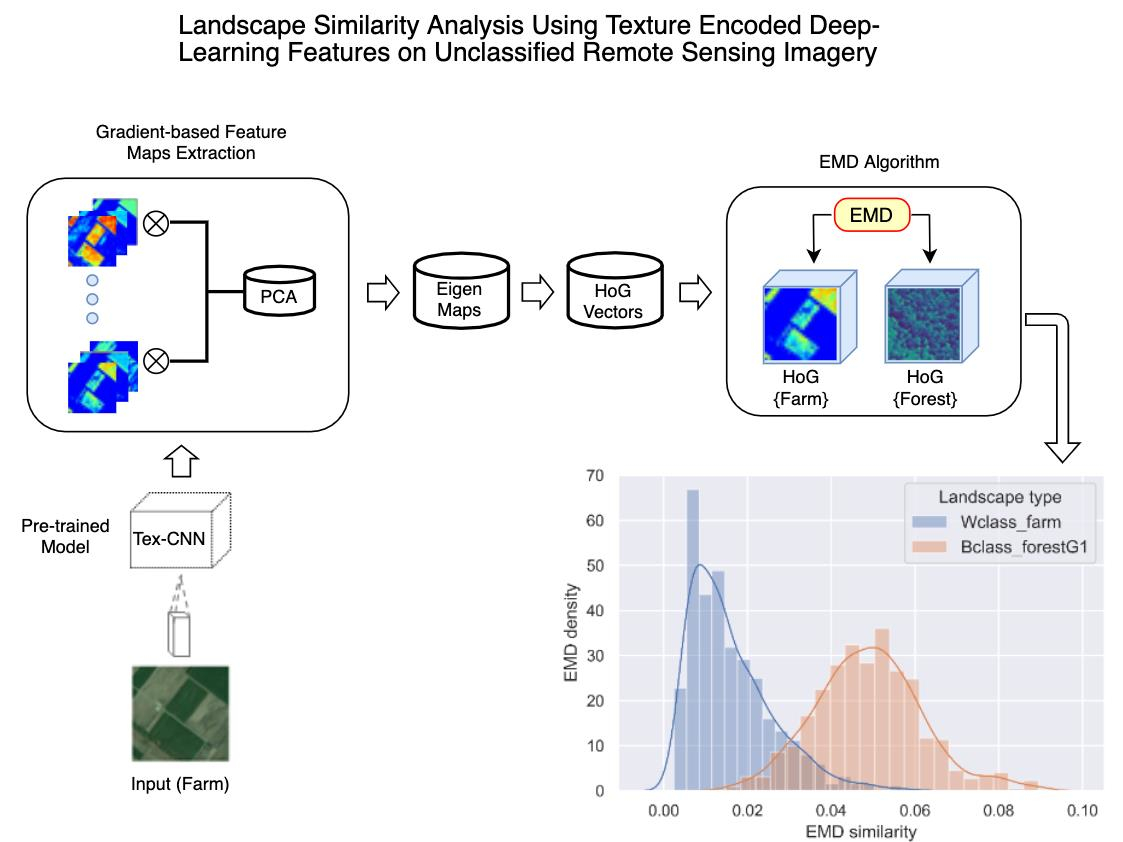
Landscape Similarity Analysis Using Texture Encoded Deep-Learning Features on Unclassified Remote Sensing Imagery

Abstract

Convolutional neural networks (CNNs) are known for their ability to learn shape and texture descriptors useful for object detection, pattern recognition, and classification problems. Deeper layer filters of CNN generally learn global image information vital for whole-scene or object discrimination. In landscape pattern comparison, however, dense localized information encoded in shallow layers can contain discriminative information for characterizing changes across image local regions but are often lost in the deeper and non-spatial fully connected layers. Such localized features hold potential for identifying, as well as characterizing, process–pattern change across space and time. In this paper, we propose a simple yet effective texture-based CNN (Tex-CNN) via a feature concatenation framework which results in capturing and learning texture descriptors. The traditional CNN architecture was adopted as a baseline for assessing the performance of Tex-CNN. We utilized 75% and 25% of the image data for model training and validation, respectively. To test the models’ generalization, we used a separate set of imagery from the Aerial Imagery Dataset (AID) and Sentinel-2 for model development and independent validation. The classical CNN and the Tex-CNN classification accuracies in the AID were 91.67% and 96.33%, respectively. Tex-CNN accuracy was either on par with or outcompeted state-of-the-art methods. Independent validation on Sentinel-2 data had good performance for most scene types but had difficulty discriminating farm scenes, likely due to geometric generalization of discriminative features at the coarser scale. In both datasets, the Tex-CNN outperformed the classical CNN architecture. Using the Tex-CNN, gradient-based spatial attention maps (feature maps) which contain discriminative pattern information are extracted and subsequently employed for mapping landscape similarity. To enhance the discriminative capacity of the feature maps, we further perform spatial filtering, using PCA and select eigen maps with the top eigen values. We show that CNN feature maps provide descriptors capable of characterizing and quantifying landscape (dis)similarity. Using the feature maps histogram of oriented gradient vectors and computing their Earth Movers Distances, our method effectively identified similar landscape types with over 60% of target-reference scene comparisons showing smaller Earth Movers Distance (EMD) (e.g., 0.01), while different landscape types tended to show large EMD (e.g., 0.05) in the benchmark AID. We hope this proposal will inspire further research into the use of CNN layer feature maps in landscape similarity assessment, as well as in change detection.

1. Introduction

Earth system and environmental data have become abundant via a variety of sources ranging from model simulation data, citizen science, amateur drones, airborne sensors, commercial satellites, and easily accessible data such as Landsat [1,2]. These data are available at unprecedented spatial and temporal resolutions and are widely used for understanding processes of environmental change across time and space. Given the rapidity of human-induced landscape disturbances, there is increasing interest in using environmental data resources to not only understand but also characterize and quantify landscape-scale disturbances, and to support decisions and policies aimed at remediating degraded landscapes [3,4].

Identifying the underlying processes that generate spatial patterns is critical to quantifying changes in patterns across space and time [5]. For instance, we ask questions like, where are degraded landscapes common? What types of specific features are common or different between geographical locations? Are the underlying processes driving pattern changes similar or different across locations? How are degraded ecosystems responding to restoration campaigns? Such questions can be addressed through landscape pattern comparison. In urban planning and land management, for example, applications that provide information on images similar to regions under investigation are essential for decision-making [6]. Traditional landscape similarity analysis tools, however, rely largely on change-detection analysis on classified landcover maps to predict or quantify process-driven changes. While these approaches have been successful, such features are limited in uncovering the complex and non-linear nature of process–pattern relationships [7]. Moreover, they are also dependent on the accuracy of the underlying map classification and incur challenges associated with legend harmonization and consistency/reproducible methods for data processing [8]. Furthermore, processes and patterns are both interdependent and affect each other in many ways, thus complicating prediction efforts [9]. As the growing historical archive of image data is increasingly being used to develop monitoring schemes and tools for understanding complex land-change processes [5], new tools capable of extracting structural information from raw, unclassified land-image data are needed.

Machine learning algorithms from computer vision research are capable of learning to extract robust descriptors from image data. Such descriptors are useful representations of data structure, and hence hold potential for landscape research [10]. For example, Tracewski et al. [11] demonstrated the application of deep learning for different landcover types characterization. Grinblat et al. [12] also applied deep neural networks for plant species identification based on vein morphological patterns. The landscape similarity search algorithm proposed by Jasiewicz et al. [13] illustrates the potential of computer vision approaches to discover (dis)similar landscapes across space. Recently, Buscombe and Ritchie [14] demonstrated that deep convolutional neural networks (CNN) account for spatial context and hence are effective for classifying spatially structured datasets. Thus, CNN models can be considered a recent class of spatially explicit models [15].

Computer vision models, such as CNNs, contain filter banks which engage in spatial learning, to extract spatially discriminative features of increasing complexity through weight-sharing [16]. Lower CNN layer feature maps contain local information that captures fine-grain discriminative patterns useful for similarity mapping, while deeper-layer features lack geometric invariance, which weakens their robustness to map finely detailed landscape patterns across variable scenes [17]. The layers of CNNs can preserve representative information about an input image with varying rotation and illumination [18]; consequently, pretrained CNNs can be employed to extract features for characterizing dynamic texture and dynamic scenes [19]. CNN filters demonstrate consistent response to useful local regions of images; based on this property, Li et al. [20] proposed a PatternNet that utilizes deconvolution (i.e., up-sampling) to discover discriminative and representative patterns in images. In a related study, Lettry et al. [21] introduced a model capable of detecting repeated patterns in images. The authors provide evidence that consistent small patterns can be strongly expressed in the shallower layers and hence are detected as major repetitions. Given the importance of texture in landscape aerial scenes, these properties may be particularly useful in recognizing different types of landscape scenes in aerial and satellite image data.

A variety of CNN architectures have been proposed to resolve image-classification problems in recent years [22,23]. CNN layer depth, input size, and even training strategies adopted may influence the model performance and competitiveness with traditional machine learning techniques [24]. For instance, to learn multi-scale features which are robust to scale variation, and thus reduce misclassification rates, Liu et al. [25] proposed a method in which randomly cropped image patches are used for model development. Gong et al. [26] also introduced a saliency-based feature extraction framework with anti-noise transfer network and found the approach to yield high classification accuracy on benchmark datasets. CNNs with feature concatenation or fusion modules are simple but effective feature extraction frameworks that have been adopted to combine local and global image features for improving the performance of many scene classification and other pattern recognition tasks [27,28,29]. Ye et al. [30] presented a multi-stage model that extracts and fuses low-, middle-, and high-level features, and obtained 95% accuracy on the Aerial Image Dataset (AID). Kang et al. [31] also developed a network that captures contextual information via the fusion of deep and shallow features to improve ship-detection accuracy. A framework with dilated convolution and skip connections was found to learn multiresolution discriminative features for scene classification [32]. Similarly, Gao et al. [33] proposed a network in which feature maps generated from input images are passed on to a concatenating layer, forming a combined feature map with richer discriminative information. The authors concluded that their method significantly improved hyperspectral image classification. In a related study, Huang and Xu [34] used weighted concatenation to combine features across all CNN layers, yielding overall accuracy of 95% in AID. Similarly, Zeng et al. [35] developed a two-branch CNN in which local and global features are independently extracted and concatenated. With extensive experiments, the authors demonstrated that feature concatenation resulted in over 90% accuracy for most scene classes in AID.

Despite the state-of-the-art performance of current CNN architectures, deep learning algorithms are generally perceived as “black-boxes” in both computer vision and across other domains; consequently, there have been intensifying calls to interrogate and reveal the inner workings of deep learning models in disciplines such as geography [36]. Visualizing spatial attention maps (i.e., feature maps) is a fairly simple method of exploring how CNNs learn and make decisions on an input image. The approach may be gradient-based and involve computing network output changes with respect to input [37], or utilizing a deconvolution network that projects image features over a plane [38]. Zhou et al. [39] also proposed converting the linear decision (regression) layer into a convolutional layer for generating class-based attention maps. To improve gradient-based feature map quality, guided backpropagation has also been introduced [40]. As these approaches do not always produce class-specific feature maps [41], Selvaraju et al. [42] proposed Grad-CAM, which integrates guided backpropagation and class activation maps, and thus yielding class-discriminative spatial attention maps. In a related research, Omeiza et al. [43] proposed Smooth Grad-CAM++ to improve the spatial resolution and localization of patterns in feature maps. Class-selective relevance mapping has also been proposed to derive feature maps that contain the most discriminative regions of interest in medical images [44].

In this study, we focused on gradient-based convolutional feature maps. Gradient with respect to an input image, is a sensitivity map measuring how changes at an input pixel spatial location affect changes in CNN model predictions [42]. Given an input image, if small changes to its pixels correspond to a large network output change, then it follows that such pixels encode “significant” spatial information. The above novel approaches to visualize and interpret CNN feature maps have been used extensively to evaluate and improve models’ performance. However, we consider such CNN features to have potential for image similarity matching and retrieval. For example, a global representation vector extracted from a CNN has been shown to improve object-image retrieval on Oxford and Paris datasets [45,46]. As demonstrated in recent studies, CNNs with feature concatenation framework incorporate fine-grain textural details which encode relatively significant discriminative patterns [27,28]. Traditional CNN architectures, on the other hand, tend to focus largely on processing input images and feature tensors from individual layers. Thus, traditional CNNs have the tendency to discard tangible proportions of original image texture, as well as CNN layer features that contain discriminative information. To this end, we propose training and deploying a texture-encoded CNN model (Tex-CNN) to evaluate landscape similarity. Our Tex-CNN is a simple, yet computationally efficient feature concatenation architecture for generating discriminative feature maps. In order to compare our proposal with existing techniques, a classical CNN was trained. Using the trained Tex-CNN and the classical CNN, we derived feature maps, to compare different or repeating spatial patterns across space. Given the discriminative learning behavior of convolutional filters, feature maps are sometimes sparse; to reduce the CNN feature maps to a compact representation that best encodes patterns in a given landscape, principal component analysis (PCA) was further performed, and feature maps with the highest eigen values were selected. The histogram of oriented gradients (HoG) vector was then extracted from each map for comparison using the Earth Movers Distance (EMD) algorithm.

The contribution of this study is, therefore, two-fold. (1) A gradient-based convolutional feature map approach to landscape similarity analysis was proposed. Using gradient-based features, the proposed landscape similarity assessment utilizes significant spatial patterns in a query and a candidate image for comparison. (2) A landscape similarity metric capable of detecting within- and between-landscape types was developed. The proposed metric effectively discriminates farm landscapes from mountainous, as well as forested, landscapes. The paper is arranged as follows: We first illuminate the importance of spatial feature maps in landscape comparison; next, the methodological pipeline is presented, followed by results, discussion, and conclusion.

2. Related Work

Prior to the emergence of state-of-the-art of CNNs capable of detecting and classifying objects and patterns, image texture processing was one of the earliest applications in which CNNs were employed to extract discriminative local features [47,48].

2.1. Representing Patterns in CNN Feature Maps

Convolutional feature maps can be thought of as spatial activation features encoding discriminative regions within a given input image [49]. A feature map can also be viewed as detection scores resulting from the application of a filter over spatial locations in a 2D image; the activation value obtained at the i-th location quantifies the importance of the pixel at that location [50]. Such locations may be linked, at least conceptually, to “landscape features of interest” or those areas of the landscape that are discriminative of the landscape scene label. The potential of a convolutional-feature-based approach in urban landscape change detection was presented in El Amin [51]. The authors demonstrated that CNN features can perform higher than “hand-crated features” and other state-of-the-art techniques. In related research, Albert [52] showed that features extracted from CNNs trained discriminatively on urban imagery effectively compare neighborhood similarity across European cities.

In landscape research where local-to-global changes or pattern similarity are sometimes of interest, CNN maps can be helpful. Feature maps represent local response regions of filters and thus encapsulate valuable pattern information [41]. These local regions also encode information pertaining to the underlying pattern-generating process. Feature maps from convolutional layers represent local descriptors of particular image regions which can be aggregated into global descriptors for image retrieval [53]. An image-retrieval framework is also closely related to the landscape-pattern comparison problem. For instance, CNN activations containing pronounced spatial information can be utilized for detecting repeated patterns [21]. The challenge to detect repetitive spatial patterns is similar to landscape similarity analysis problem. It has been illustrated that convolutional layer activations are local region descriptors and outperform many state-of-the-art descriptors [48,49]; thus, if these feature maps are well-pooled, a compact representation of a given landscape can be derived. Additionally, Zagoruyko and Komodakis [41] have shown that feature maps represent “knowledge learned” by a given network about the underlying pattern and can be transferred to other networks, to improve pattern detection. Furthermore, classical machine-learning algorithms for pattern detection or classification, such as Random Forest, Support Vector Machine, and Maximum Likelihood being employed in landscape research, can be coupled with deep feature extraction models to boost performance [54]. For example, it has been shown that feeding features from CNNs to other models improve results [29]. We therefore postulate that CNN-feature-based frameworks hold the potential to enable the detection and quantification of spatially patterned processes.

2.2. CNN-Feature-Based Image Retrieval

Image retrieval is an active research area in this era of “big data”, where the objective is to find a set of images that are the most similar to a given query image. Content-based image retrieval (CBIR) is a widely applied technique for retrieving images in databases. In CBIR, low-level image descriptors (e.g., color, texture, and structure) are extracted to form an image representation; a suitable measure is then selected to estimate similarity between images. Several algorithms have been proposed for an improved CBIR. For example, Unar et al. [55] combine both visual and textual features for image retrieval. Zhang et al. [43] also developed an algorithm that segments an image into salient, non-salient, and shadowed regions, in order to extract spatially relevant information. Earth observation data now available in various archives could provide a wealth of information through effective search and retrieval techniques [6].

Recent research has shifted towards the use of features extracted from deep convolutional layers of CNNs for image matching and retrieval [46,56]. The use of deep convolutional features for image retrieval is demonstrated in a study conducted by Babenko et al. [53]. Chen et al. [45] propose region-of-interest deep convolutional representation for image retrieval. Their approach first identifies regions of interest and proceeds to extract features from the fully connected layer. Shi and Qian [46] also adapted the region-of-interest-based approach called strong-response-stack-contribution, by exploring spatial and channel contribution, to generate a more compact global representation vector for an object-based image retrieval challenge. Cao et al. [50] applied adaptive matching by splitting feature maps and later spatially aggregating them into regions of interest for comparison. Liu et al. [57] proposed extracting and pooling subarrays of feature maps as local descriptors for visual classification task and found that the method outperforms features from fully connected layers. The aforementioned applications hold potential for designing resource management and decision-making applications in geography.

3. Materials and Methods

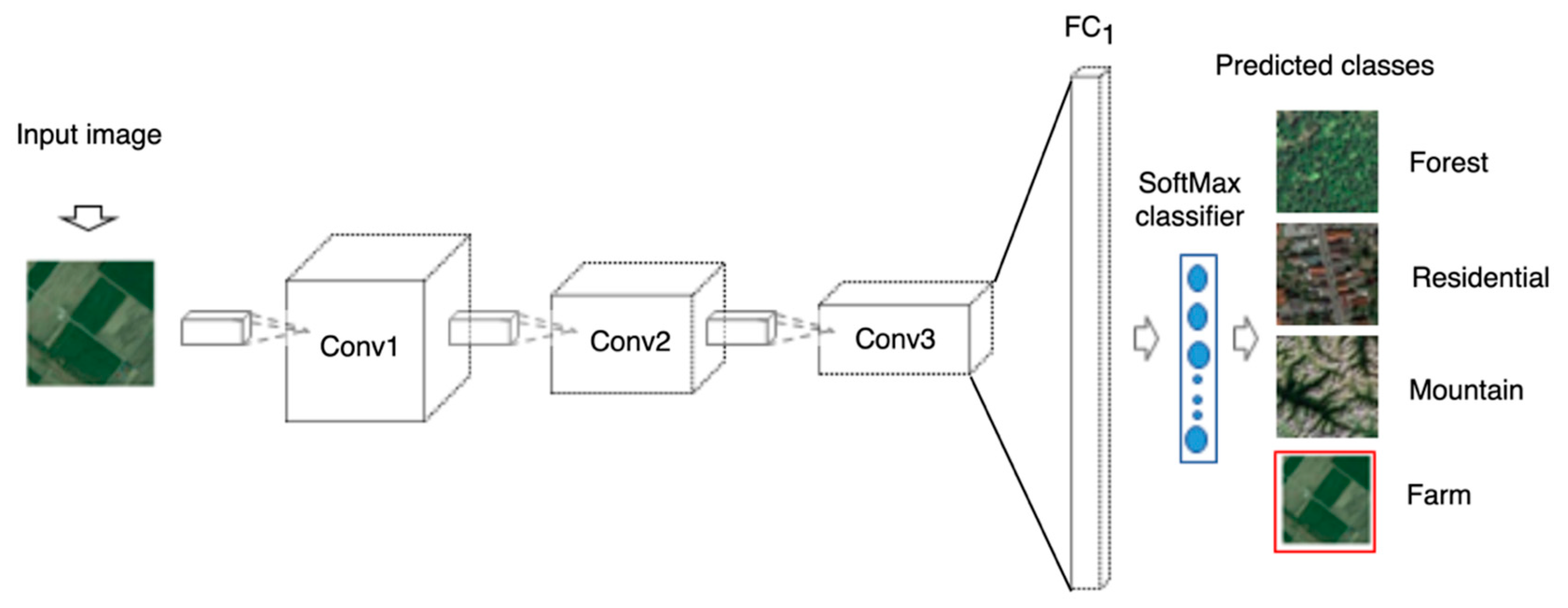
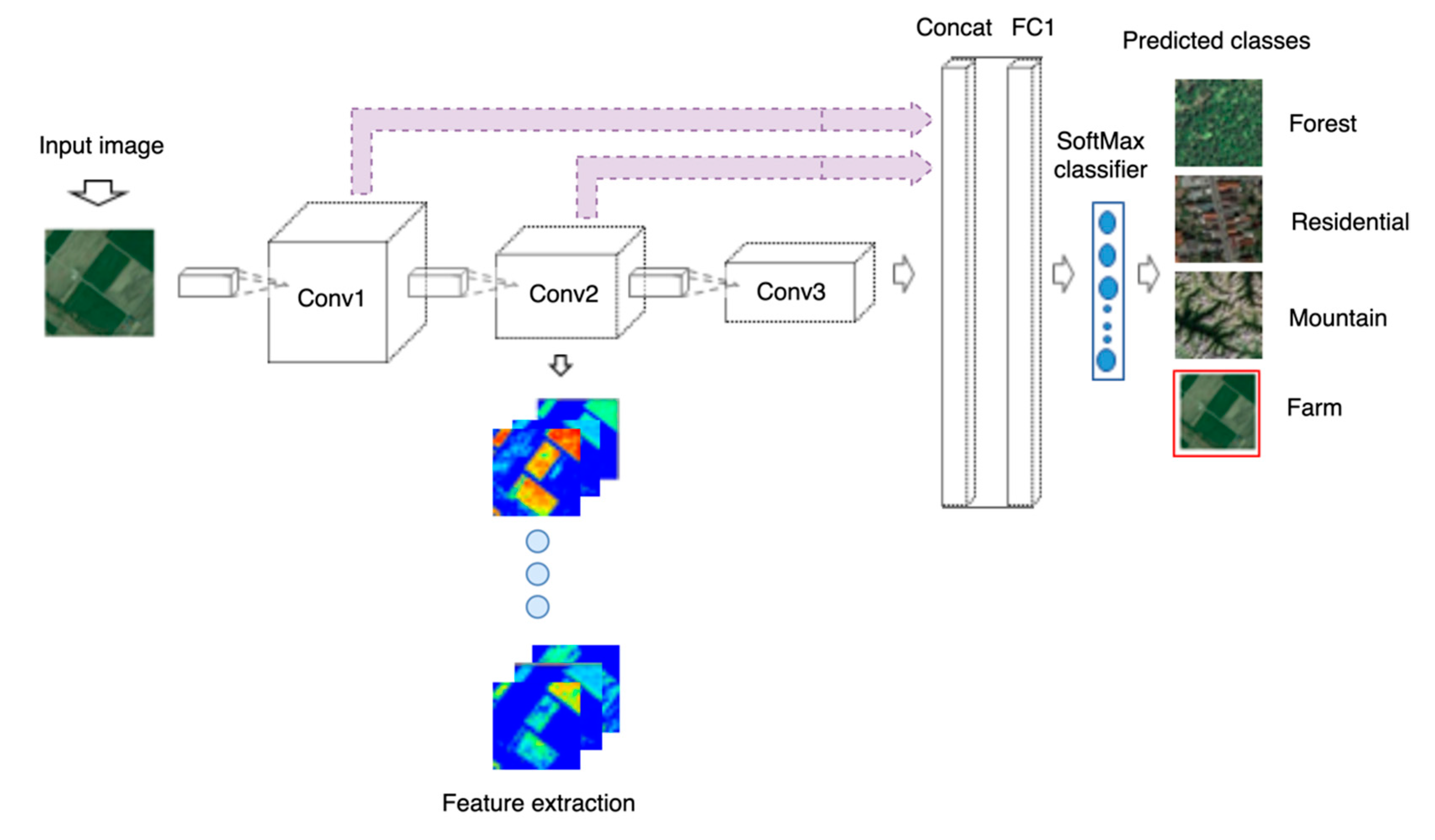
3.1. Models’ Architecture

In the context of landscape similarity mapping, global shape information present in fully connected layers is of less significance, as landscape patterns often lack unique or stable geometry across space. Given that lower layers capture local patterns [16], we concatenated multi-layer features, to learn a discriminative representation of the data-generating process. In feature fusion, feature maps from three convolutional layers (i.e., conv1, conv2, and conv3) are concatenated followed by flattening into feature vectors to yield a dense layer (denoted FC1). One possible approach to improving CNN features’ discriminative potential is to apply attention pooling strategies that takes the weighted sum of different feature maps instead of concatenating features, as this technique exponentially increases model parameters as well. However, we adopted feature concatenation, as it has been proven to enable the extraction of multiscale features, potentially obviating the need for multiscale inputs during model development [58]. Moreover, attention strategies are effective for object recognition tasks but may not tangibly improve landscape pattern discrimination.

Work similar to our approach is the Andrearczyk and Whelan [59] feature concatenation framework. Figure 1 illustrates the architecture of a classical CNN, while Figure 2 depicts our model architecture. For model design, we build on the VGG16 model architecture and filter constellation [60]. Thus, 32, 64, and 128 Filters are used in the first, second, and third convolutional layers of the classical CNN and the Tex-CNN models. The proposed model architecture is intended to be simple with minimum parameters as possible for field deployment. A model with fewer than three convolutional layers does not only limit the number of feature maps available for exploration but may not be able to shatter the training data as well. Given the data at hand, models with over four convolutional layers could potentially pose overfitting challenges.

3.2. Model Parameterization and Training

We opted for training our models from scratch, as this approach gives flexibility over model architecture. Although there is potential for data limitation, as well as over-fitting, in this framework [61], the approach facilitates feature maps comparison, as it ensures that features are the direct result of filters learned on data presented to models, compared to using pretrained networks in which filters learned from an entirely different domain than the task at hand. Given that the input image size is large enough (i.e., 225 × 225), we selected 7 × 7 convolutional kernels and used a fixed filter size with stride 1 throughout the convolutional layers. Filter receptive field size changes with layer depth and could result in profound differences in feature spatial resolution between successive layers. In the pooling layers, 2 × 2 max pooling with stride 2 is applied. The receptive field size at the third convolutional layer, therefore, becomes 46. We utilized 75% of the sample data for training and 25% for validation. To mitigate potential overfitting, 25% drop-out is used in convolutional layers, while 50% is applied to the FC1 layer [62]. The rectified linear unit (ReLU) is used as the activation function. Multiclass cross-entropy loss function is employed, and the models are trained for 30 iterations with Adam as the optimizer. Adam adaptively computes and updates gradients and is invariant to diagonal scaling of gradients [63]. The Keras-Tensorflow backend was used for building and supporting computations required to train the CNN models on a GPU with a NVIDIA-supported graphics card.

Table 1. A summary of models’ architecture and parameters.

Layer Name	Convolution	Max-Pooling	Activation	Drop-Out
Conv-1	7 × 7 × 32	2 × 2	ReLU	25%
Conv-2	7 × 7 × 64	2 × 2	ReLU	25%
Conv-3	7 × 7 × 128	2 × 2	ReLU	25%
FC1	No	No	SoftMax	50%

summarizes the models’ architecture and parameters.

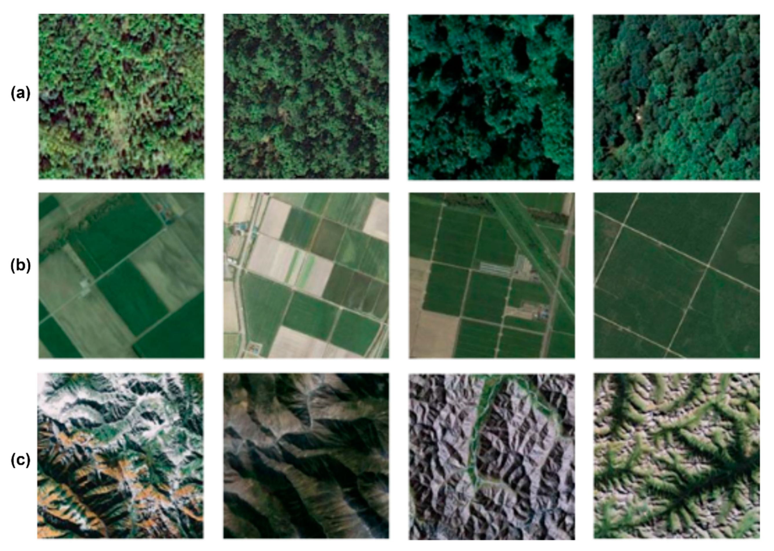
3.3. Application Context: Landscape Comparison

Unclassified imagery, which is now ubiquitous due to the availability of sensors of varying types, offers the potential for landscape similarity queries. While land-cover classification in which pixels are labeled (classified) or objects are segmented and characterized is a predominant use of aerial and satellite imagery [64], in this modeling framework, we focus on characterizing whole scenes or landscapes. An implementation of this would be helpful for automating image retrieval and potentially provide a basis for mixed scenes and/or novel land-scene categories and/or descriptors. A conceptual representation for comparing unclassified images (aka landscapes/scenes) is depicted in Figure 3, using three landscapes/scenes denoted as X, Y, and Z, but the representation is expandable to multiple landscape types. Given an image, the feature map will be extracted for comparison, using EMD. EMD(X, X’), EMD(Y, Y’), and EMD(Z, Z’) compute within-landscape similarity, while EMD(X, Y), EMD(Y, Z), and EMD(Z, X) estimate between-landscape similarity.

Benchmark datasets have long been used in computer vision for model development, due to the scarcity of labeled data, and the laborious processes required for generating such datasets, yet they remain relatively rare in geospatial research. The aerial imagery dataset is composed of high-resolution benchmark data recommended for training scene classification models [65]. The AID contains multi-resolution images; the pixel spatial resolution varies from about half a meter to eight meters, providing a suitable dataset for training classical CNN and Tex-CNN models. A common protocol in computer vision is to split a given dataset into training, validation, and test samples. This may sometimes result in high-accuracy reports resulting from overfitting. Owing to this caveat, and the need to find models capable of generalizing over a range of datasets for field application, we propose carrying out further validation by using a dataset from an entirely different sensor. As such, we employed Sentinel data to evaluate the generalizability of the developed models.

Table 2. Data types and specific application.

Data Source	Attribute	How Data Is Utilized	No. of Images
AID	Aerial imagery, pixel resolution vary between 0.5 and 8 m	Training and testing models, and building similarity distributions	9000 images used training (75%) and validation (25%). 900 images used for testing (e.g., deriving confusion matrix)
Sentinel data	Open-source satellite data; 10 m pixel resolution	Visualizing feature maps in medium resolution imagery Demonstrate potential application in Sentinel dataset	600 images used for testing and computing confusion matrix. Image tiles are extracted from sentinel scenes at different spatial locations

describes the datasets utilized in this study.

3.4. Data Augmentation

The AID consists of diverse landscape types; however, considering only three landscapes reduces the sample size. CNNs are “data hungry” models; thus, training such models from scratch by using fewer samples and classes is likely to pose data limitation issues and overfitting. We therefore attempt to circumvent this challenge via the application of data augmentation. To that end, we employ the Keras image data generator API to augment our training dataset. Given that the AID is multiresolution–image pixel sizes vary from about half a meter to eight meters, scale representation challenges are inherently reduced such that scale transformations may not make substantial difference following data augmentation. Bearing this in mind, horizontal flips and rotations (i.e., 45–180 degrees) were applied to generate enough training data. Three-thousand samples were generated for each landscape type, and thus yielding 9000 samples for the three landscape types: farm, mountain, and forest. A Sentinel dataset was used to test the potential generalizability of the method on medium-resolution satellite imagery. Figure 4 illustrates samples of AID landscapes used in our experiments.

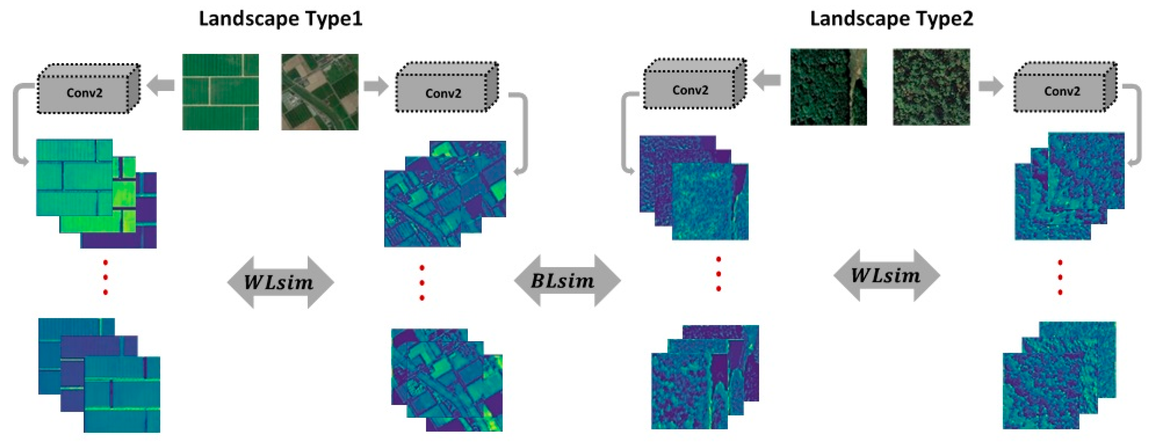
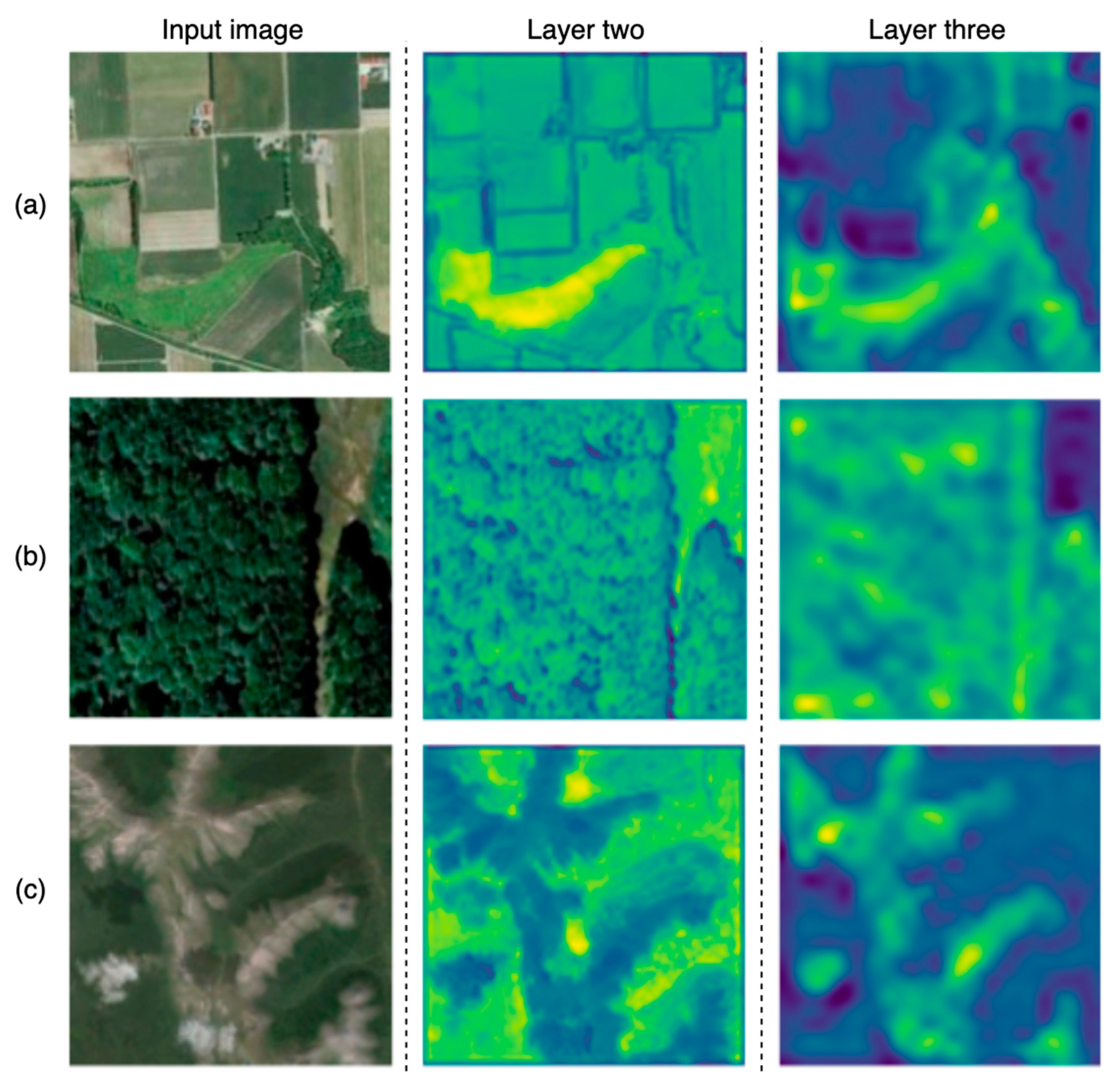
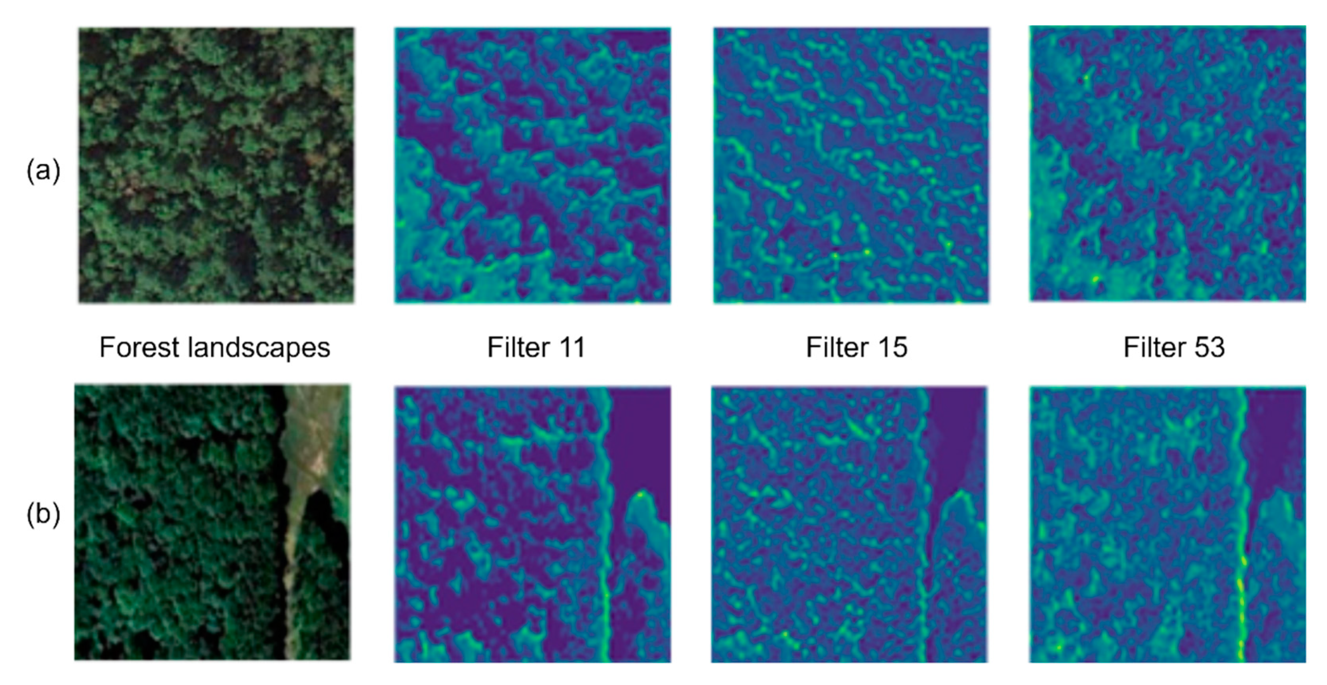
3.5. Activation/Feature Maps Derivation

Given a trained CNN model, gradient-based activation maps can be computed to allow for visualization of localized regions in an image that contribute significantly to a given output pattern. Using our trained classification model, activation maps are derived via backpropagation of filter responses to input pixel intensities [42]. ReLU is employed to constrain the backpropagation process to propagate only positive pixel values that activate filters; these pixel positions contain the highest weight and are therefore said to encode “significant patterns” or represent the signatures of the underlying pattern-generating process.

The gradient-based class activation map proposed by Selvaraju et al. [42] is derived as follows: Let $Y^c$ denote the score for a particular landscape scene. The gradient, with respect to $Y^c$, is formulated as $\frac{\partial Y^c}{\partial A_{ij}^k}$. $A^k$ denotes a set of CNN activation maps, and (i, j) are locations of pixels in the feature maps. Equations (1) and (2) summarize feature maps derivation.

$$\underset{Feature map weight}{\underbrace{{\alpha }_k^c}}\stackrel{Global average pooling}{= \overbrace{\frac{1}{Z}{\displaystyle \sum }_i{\displaystyle \sum }_j\underset{\begin{array}{c}Backpropagation gradient\\ \end{array}}{\underbrace{ \frac{\partial Y^c}{\partial A_{ij}^k}}}}}$$

(1)

$$L_{feature map}^c=ReLU \left({\displaystyle \sum }_k{\alpha }_k^c{A}^k\right)$$

(2)

The weight term ${\alpha }_k^c$ captures the “significance” of feature map k for a target landscape type/scene. ReLU is applied to the weighted sum of feature maps, yielding heat-maps whose local regions highlight the most discriminant patterns in images. The resultant CNN activation maps pinpoint locations where the model focuses its attention on, since such locations contain significant spatial patterns. Therefore, activation maps can be referred to as “saliency maps” or “spatial attention maps”.

3.6. Extracting HoG Vector from Feature Maps

For each landscape type, 50 scenes across different locations were selected for feature map extraction. We note that, since the number of filters in the second convolutional layer from which the feature maps are computed is 64, each image correspondingly yields 64 feature maps. We perform spatial filtering by using PCA to reduce the number of feature maps per image. PCA reduces feature map dimensionality, yielding a more compact image descriptor [53]. Such a step is inevitable when CNN feature maps are being compared; due to discriminative learning, not all filters respond to input images or pixels, and, as such, certain feature maps may contain no features/patterns where a filter is not activated by an input image [66,67,68]. Using PCA, a feature map (i.e., eigen map) that has the highest eigen value is selected. Next, the HoG vector is extracted from each landscape type feature map. HoG has been shown to extract effective image descriptors for pattern recognition tasks. For example, human face recognition across standard datasets is found to improve, using HoG descriptors [69]. In related research, different plant species were effectively recognized from leaf patterns, using HoG descriptors [70]. Setting the spatial parameters (i.e., cell size and cells per block) for extracting HoG features, however, requires a careful approach. In our implementation, the HoG vector is extracted by considering cell size 24 × 24 dimension and cell-per-block = 2 × 2 of each feature map. We deploy the EMD, a multivariate histogram distance measure, proposed by Rubner et al. [71], to compare the resultant HoG vector representing reference and test feature maps.

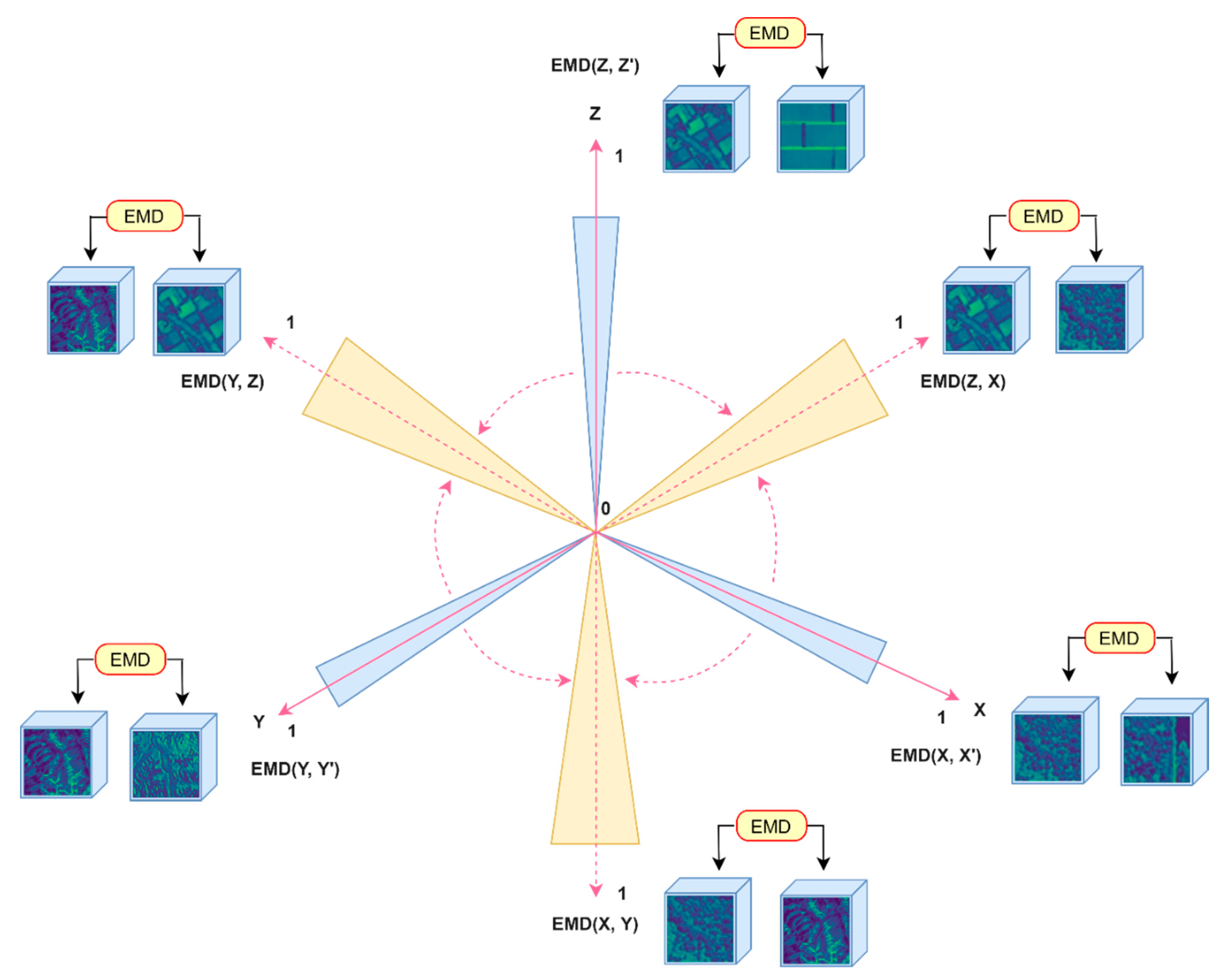
3.7. Formulating the Feature Map Comparison Metric

In the literature, there are a variety of pattern similarity comparison metrics, yet it is challenging to find robust and generic metrics to rely on when it comes to landscape similarity comparison. In this section, we illustrate how our convolutional feature map comparison metric was derived. Figure 5 is a depiction of our proposed convolutional feature-based landscape similarity comparison.

Equations (3) and (4) illustrate our formulation and computation of within- and between-landscape similarities.

$$WLsim=EMD\left(HoG\left(L_{L1 type, locX}\right), HoG\left(L_{L1, locY}\right)\right)$$

(3)

$$BLsim=EMD\left(HoG\left(L_{L1 type}\right), HoG\left(L_{L2 type}\right)\right)$$

(4)

where $L_{L1 type}$ and $L_{L2 type}$ represent different landscape categories from different spatial locations. $WLsim$ and $BLsim$ denote within- and between-landscape type comparison, respectively. For $WLsim$, we compare similar landscapes; example $L_{L1 type}$, but from different locations (e.g., $locX vs. locY$). For example, to compare farm landscapes, $locX$ will represent a reference landscape, while $loc{Y}_{\left(1,2,3\dots , n\right)}$ denotes farm landscapes (e.g., 225 × 225 grids) from other locations of interest. Landscapes whose spatial extents are large could be tiled into spatial grids of equivalent dimension as the model input size for comparison.

$BLsim$ involves a comparison of two disparate landscape types (e.g., forest vs. farm). $HoG\left( . \right)$ computes HoG feature vector, given an input feature map, while $EMD\left( . \right)$ estimates HoG feature vector similarity based on the EMD between landscapes. To test the proposed metric, 50 images from each landscape type were taken from the AID and randomly split into two subsets, thus yielding 25 images per subset, which are named G1 and G2 (e.g., farmG1 and farmG2 each contains 25 images belonging to farm landscapes). Using the metric, a compact distribution based on EMD is computed for within- and between-landscape, by comparing each scene type; for example, in farmG1, a selected scene is compared with all other scenes in farmG2. This permutation schema is repeated for all the 25 scenes in farmG1.

4. Experimental Results

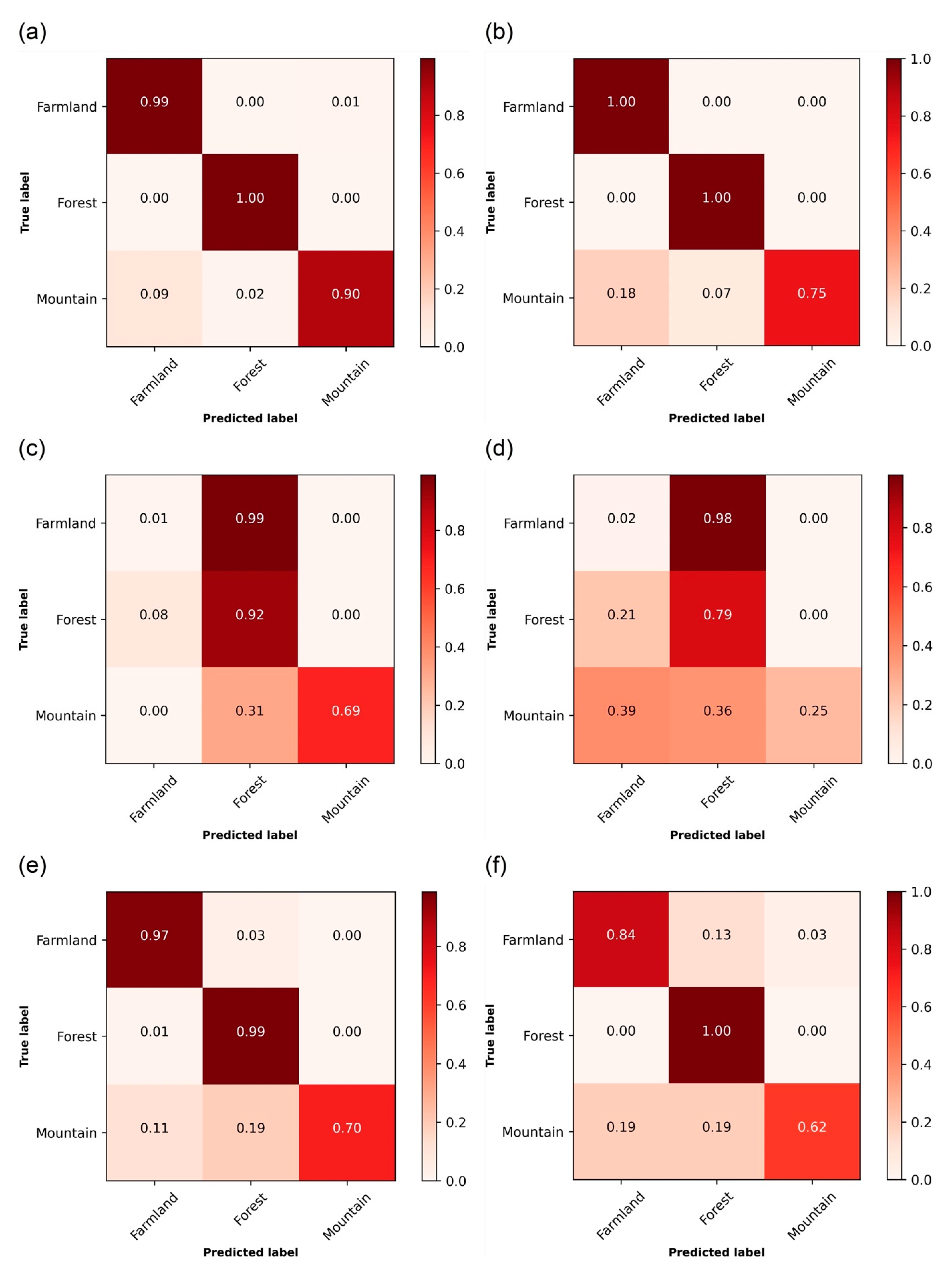
4.1. Landscape Type Prediction Models

Figure 6a–f depicts classification accuracies for landscape types on AID and Sentinel data. The confusion matrices are computed by deploying the models on the test images from AID and Sentinel datasets (i.e., 900 images for AID and 600 images for Sentinel-2). In Figure 6a,b, the Tex-CNN and the classical CNN classification accuracy reports are similar except for mountainous scenes where Tex-CNN has higher classification accuracy. In Figure 6c,d, the first row of the confusion matrix shows that over 90% of the farm landscapes are misclassified as forest in Sentinel dataset. About 70% of the mountain landscapes are correctly classified by the Tex-CNN, while the classical CNN achieves only 25% classification accuracy. Figure 6e,f shows classification accuracies after fine-tuning the models with a combination of AID and Sentinel data. It can be observed that misclassification rates for farm landscapes have been substantially reduced.

Table 3. Overall accuracy (OA) and selected per-scene class accuracy for reference and our proposed Tex-CNN on the AID.

Methods	Farmland (%)	Mountain (%)	Forest (%)	OA (%)
TEX-Net-LF [72]	95.5	99.9	95.75	92.96
Fine-Tuned SVM [73]	97.0	99.0	98.0	95.36
PMS [29]	98.0	99.0	99.0	95.56
CTFCNN [34]	99.0	100	99.0	94.91
GCFs + LOFs [35]	94.0	99.0	99.0	96.85
MF2Net [74]	97.0	91.0	94.0	95.93
Classical CNN	100	75.0	100	91.67
Tex-CNN	99.0	90.0	100	96.33

compares overall accuracy reports, as well as per-landscape type classification accuracies for reference state-of-the-art techniques and Tex-CNN on the AID. It can be seen that the Tex-CNN is highly competitive and, in some instances, outperforms other methods.

4.2. Exploring CNN Layer Features Suitability for Landscape Comparison

Given that CNN layers process inputs hierarchically, feature maps spatial resolution become coarser with layer depth: Earlier layers contain finer resolution features, while deeper layer representation gives coarser features. We conducted visual assessment of feature map quality, as well as the potential utilization of the second- and third-layer feature maps. Layer-one features were not included in this analysis, as gradient-based features cannot be computed by using input image data as the penultimate layer. Figure 7 depicts feature maps with the highest eigen values extracted from Tex-CNN. The feature maps are the result of applying PCA to layer two- and three-feature tensors. Notice how the spatial resolution changes across the layers. While layer-two eigen maps are fine-grained, with distinct patterns (e.g., farm boundaries, tree clusters), this pattern is not clearly interpretable in layer-three eigen maps. In Figure 7, row (a), layer-two shows high-resolution features with conspicuous farm boundaries. Contrarily, layer-three map depicts low-resolution features; the boundaries of individual parcels are blurred out. In Figure 7, row (b), layer-two shows fine-grained clusters of trees; layer-three, on the other hand, depicts coarse scale patterns which are not immediately recognizable as forest.

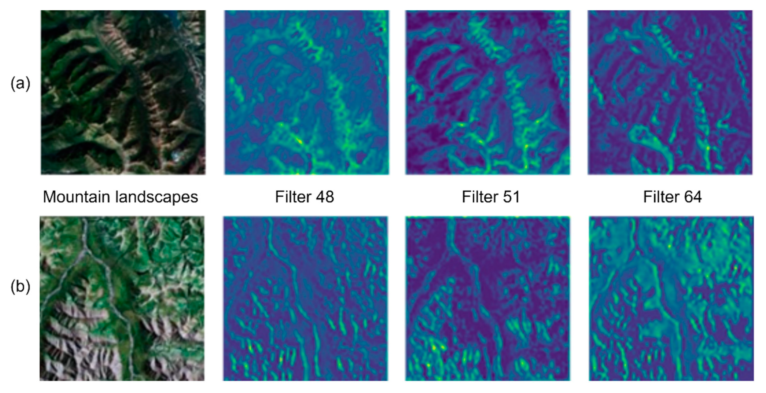
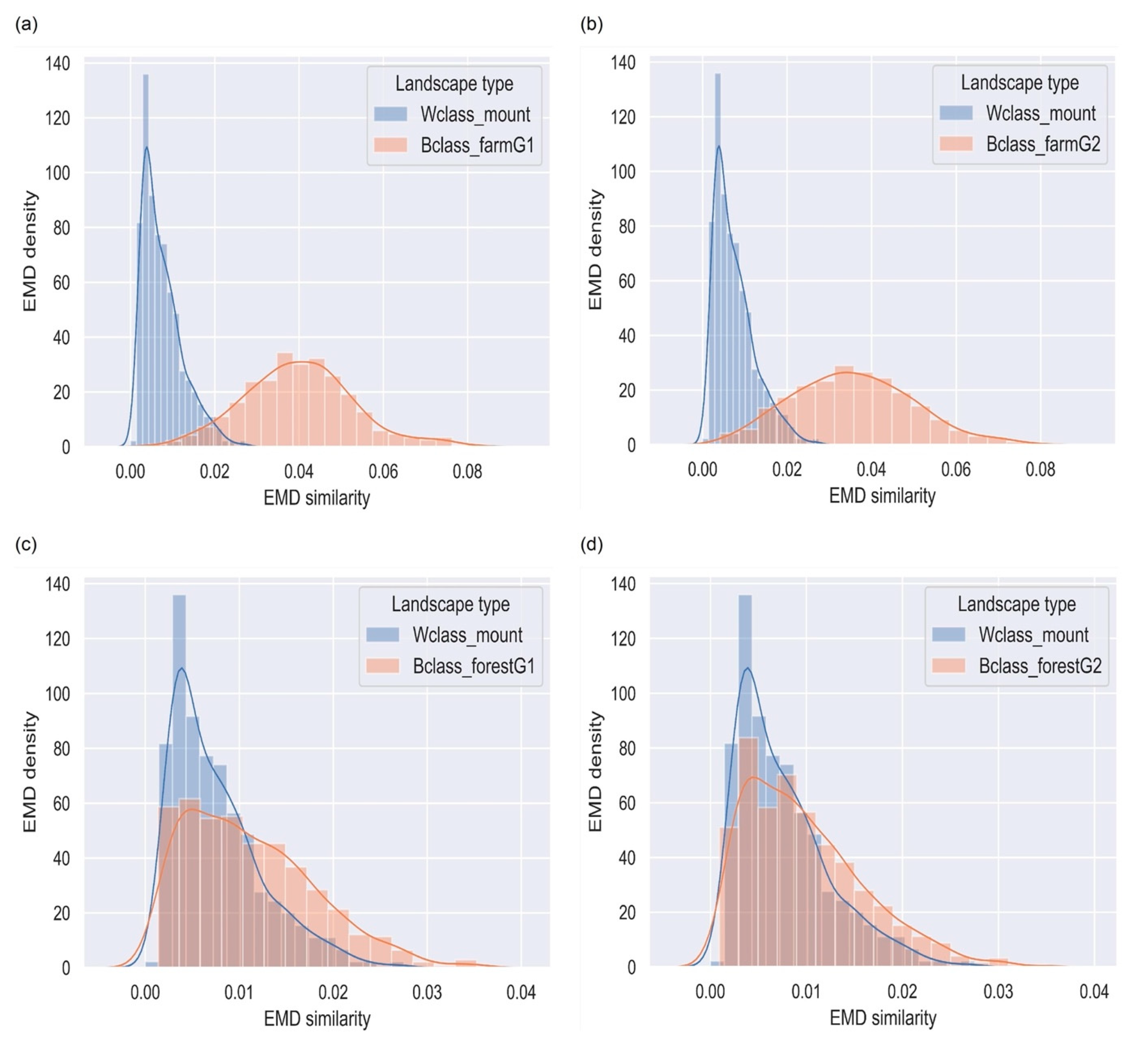
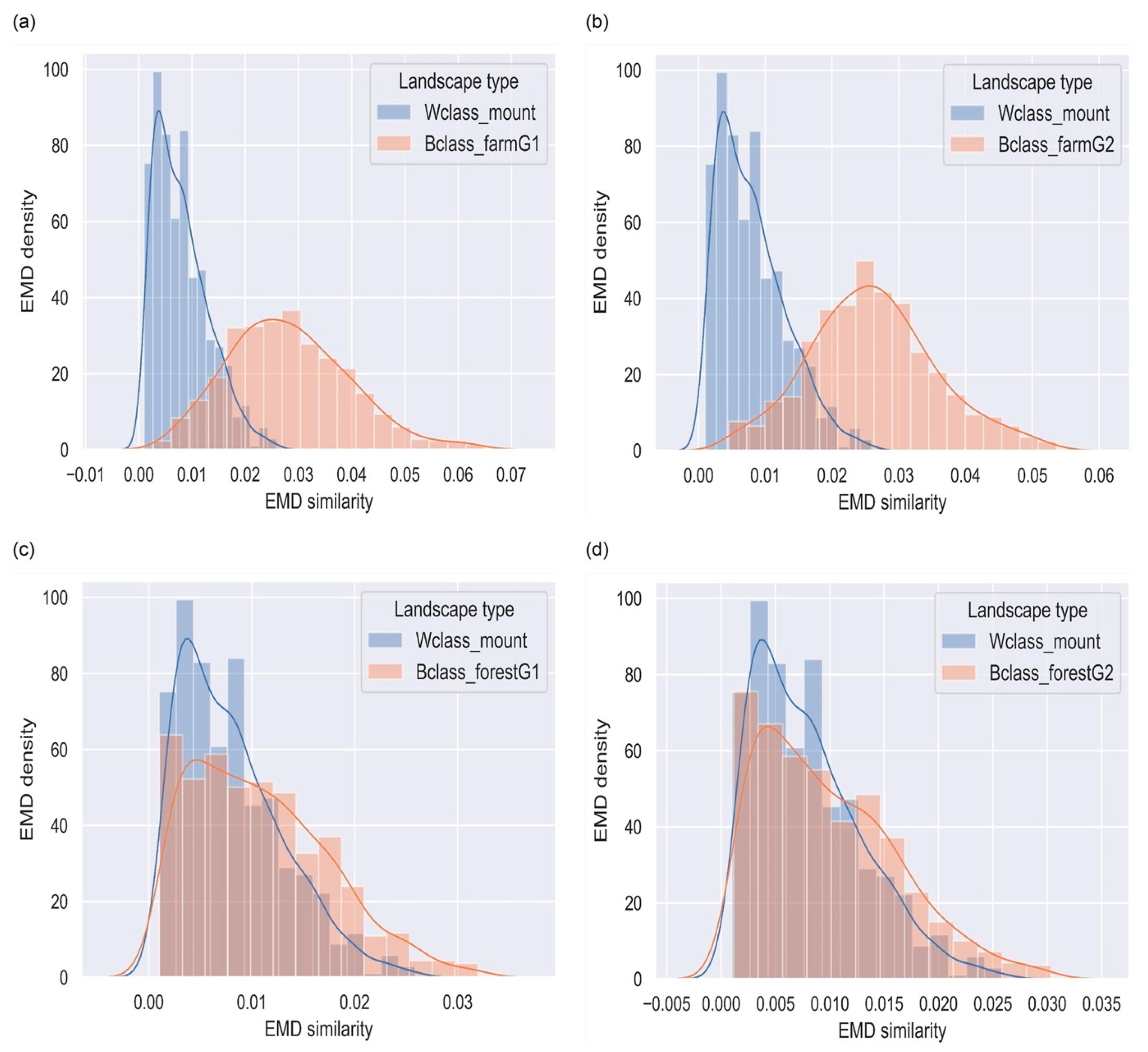
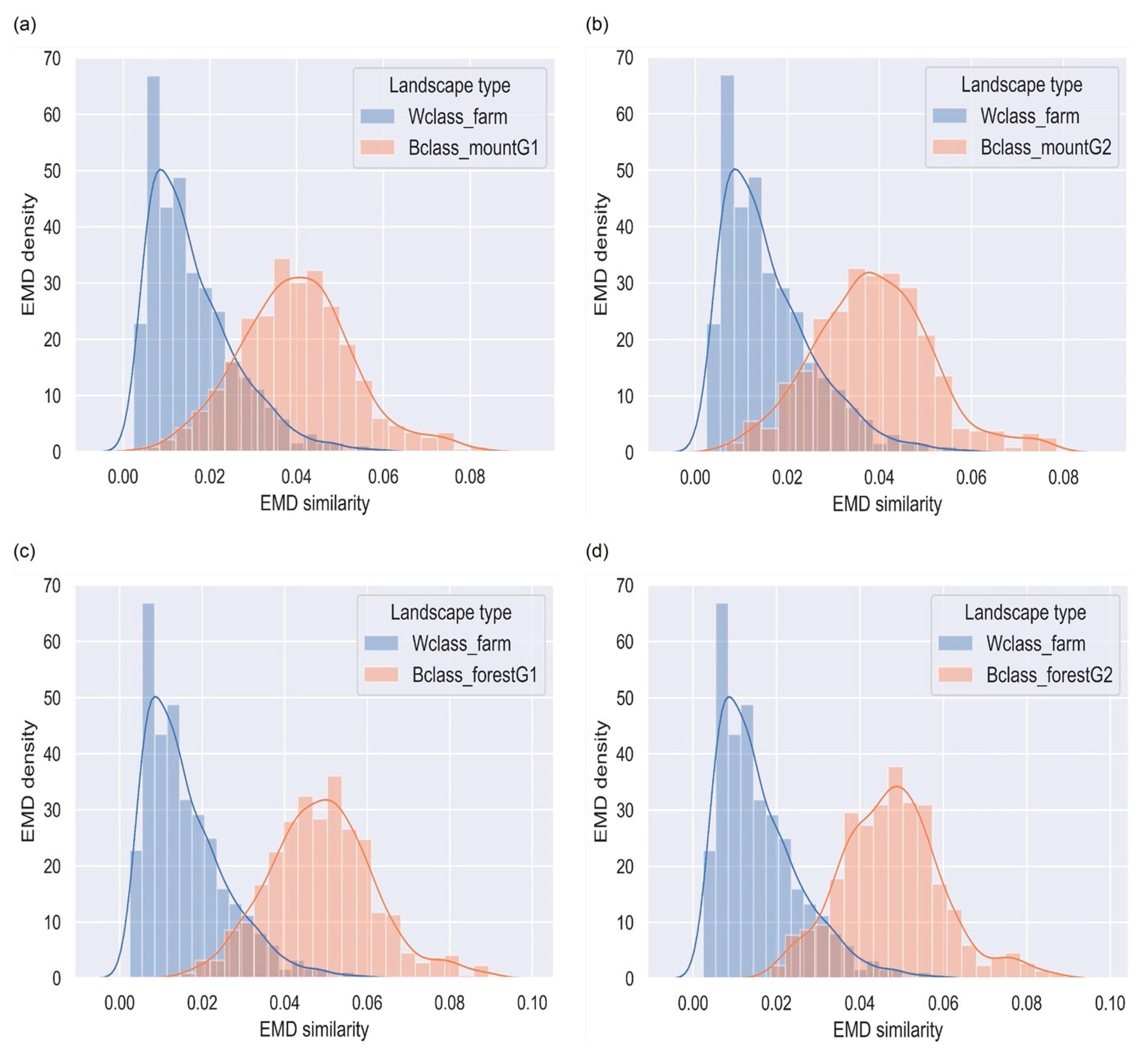
4.3. Mountainous Terrains

We hypothesized that feature maps from within-landscape types would have lower EMD values, while those originating from disparate classes would have higher EMD values. We first conducted a Kolmogorov–Smirnov test to ascertain the validity of this hypothesis. As expected, it turns out that between-class feature distributions were statistically significantly different ($p<0.001$). A sample of mountain landscapes from the AID and Sentinel datasets is depicted in Figure 8. Feature map regions that are highlighted in warmer colors represent the most significant discriminative patterns learned by the three filters; notice that most of these areas are predominantly less vegetated. Regions with cooler (blue) colors are found to be less important, according to the model’s weighting decision. Notice also that the filters sometimes perceive similar regions differently in terms of significant patterns—pixels that are found to be significant by one filter may be seen to have less weight by another filter, due to the discriminative learning behavior of CNNs.

Figure 9 shows the results for comparing mountainous landscapes and farm landscape types. It can be seen from Figure 9a,d that feature maps from similar landscapes display smaller distances, and hence their distribution falls to the left, characterized by smaller EMD. Over 60% of features in Wclass_mount of Figure 9a,b show EMD score of 0.01, while more than 50% of between class comparison yields EMD values higher than 0.05. Moreover, it can be observed that aside from shape differences, there is little overlap in the distributions of within class (Wclass_mount, Wclass_farmG1, and Wclass_farmG2).

HoG can also be extracted directly from the original data (i.e., raw images) for comparison. We demonstrate this by computing EMD over the same set of original images used for extracting CNN feature maps. Figure 10a,d presents within-class (i.e., Wclass_mount), between-class (i.e., (mountain vs. farm) and (mountain vs. forest) EMD distributions. As can be seen in the derived CNN features, the mountain vs. forest comparison poses challenges for real image comparison as well.

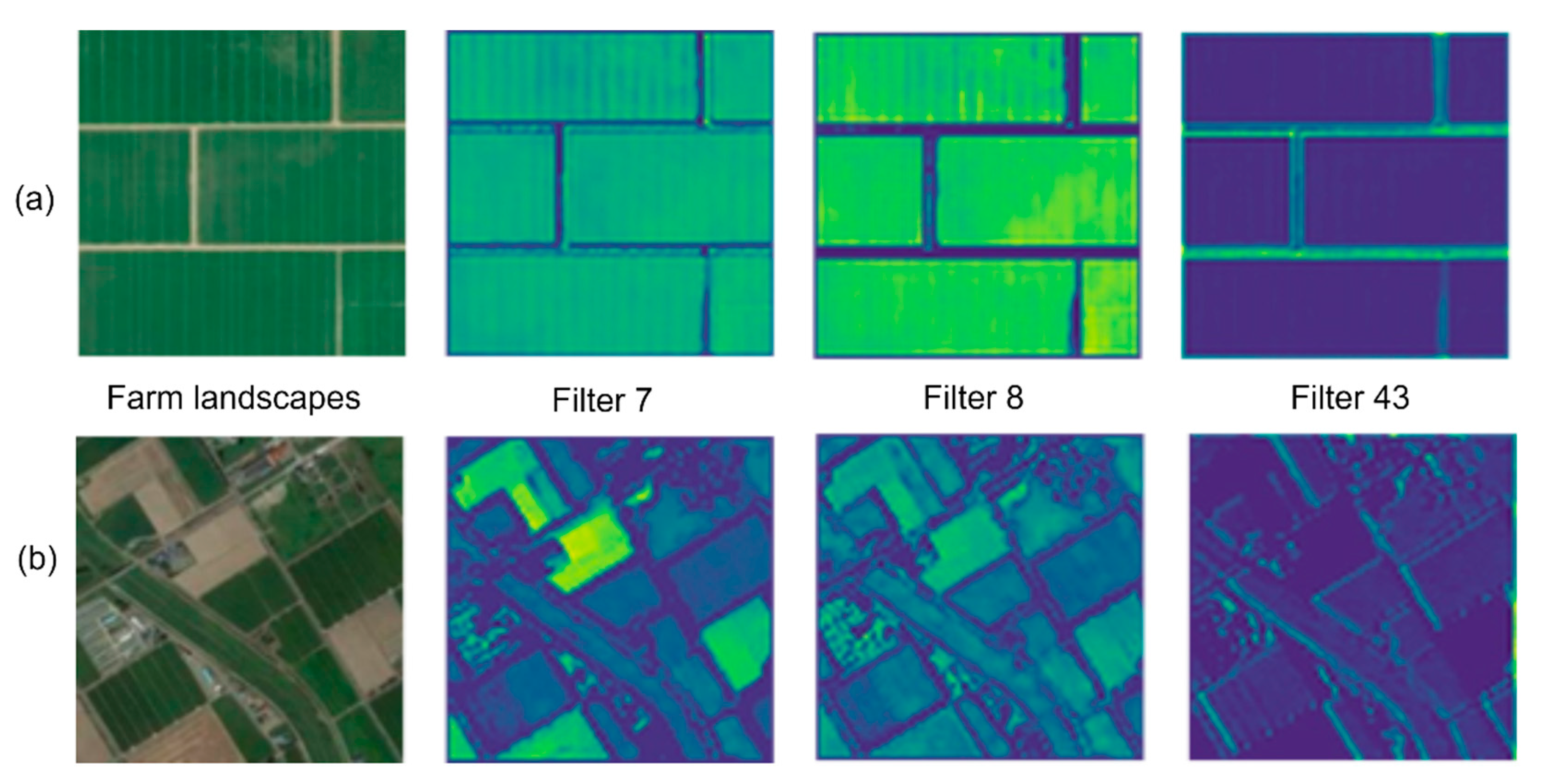
4.4. Farm Landscapes

Figure 11 presents farm landscape samples and their corresponding feature maps. Convolutional filters are randomly selected to illustrate patterns learned on farm landscape types. It can be observed that the filters specialize in detecting different features. For example, Filter 43 recognizes farm boundaries to be significant patterns, while Filter 8 weights blocks of vegetated areas higher. As shown in Figure 11a,b, the filters appear to assign significance to similar features in both AID and Sentinel datasets.

Figure 12a–d depicts within-landscape feature maps’ similarity (Wclass_farm) and between-class similarity (Bclass_mountG1 and Bclass_mountG2, for mountains; Bclass_forestG1 and Bclass_forestG2, for forests). The Wclass_farm distribution shows most feature maps with EMD values close to zero, and over 65% of the feature maps show EMD values of 0.01. Conversely, Bclass_forestG1 and Bclass_mountG1 distributions tend to fall towards higher distances, with over 50% of feature maps having EMD value of 0.05.

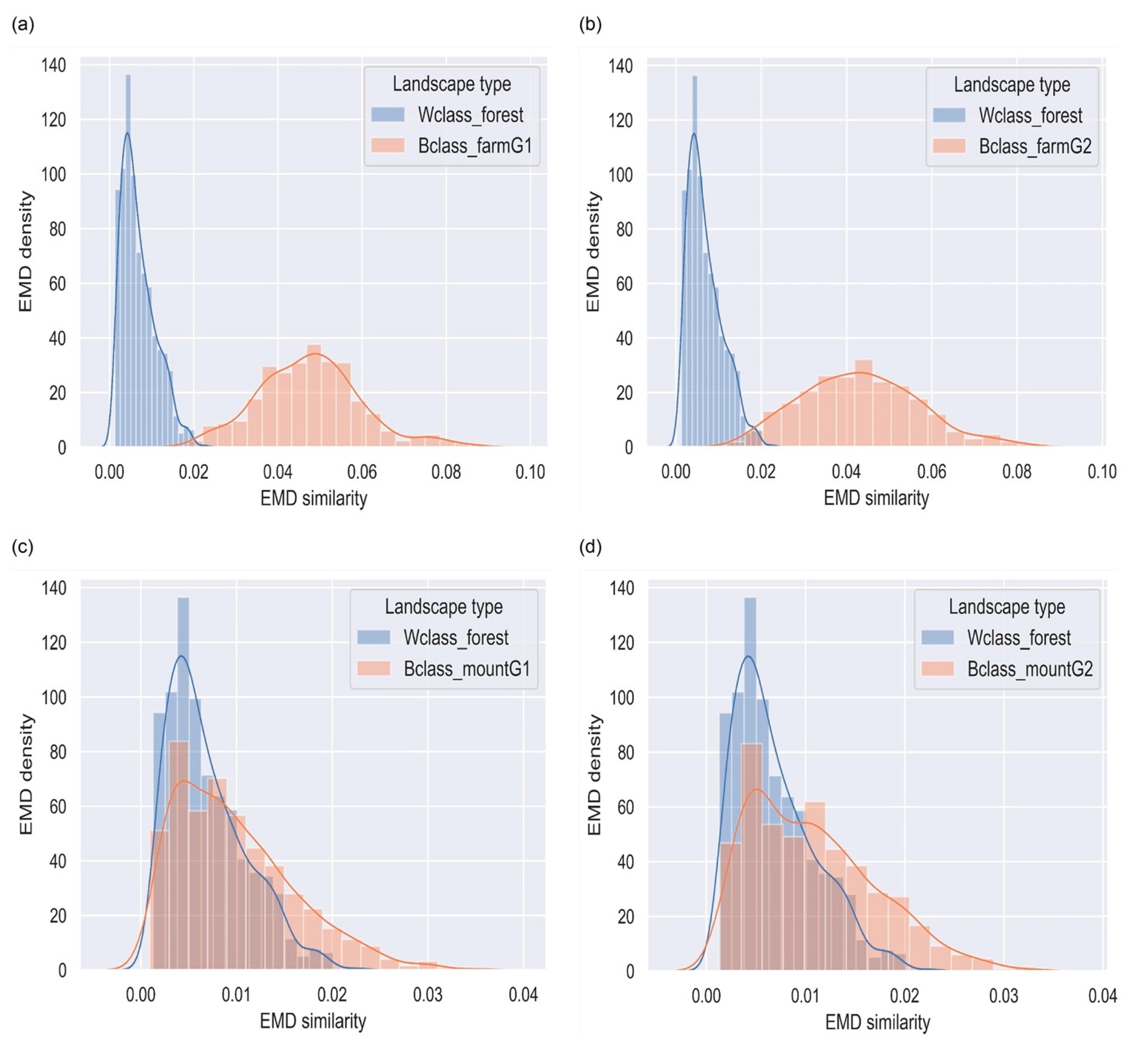
4.5. Forested Landscapes

Forest landscapes from the AID dataset and their feature maps are depicted in Figure 13a,b. Filters 11, 15, and 53 depict features at varying grain sizes, yet they represent discriminative features from an identical forest landscape.

Figure 14a,b illustrates the similarity distributions for within forest landscape (Wclass_forest) and forest vs. farm landscapes (Bclass_farmG1 and Bclass_farmG2). The two landscape types show distinct EMD similarity distribution with very little overlap. Moreover, high variance is noticeable in the between-landscape comparison. Feature maps in within-landscape comparison depict lower EMD scores, with over 60% of features showing EMD values of 0.00–0.01, while over 70% feature maps in between-landscape comparison show 0.05 EMD similarity scores. Figure 14c,d compares forest landscapes with mountains. Within-class distribution (i.e., Wclass_forest) shows lower variance and relatively shorter EMD scores. However, though the distributions depict different shapes, there tend to be substantial overlap in within-class and between-class (Bclass_mountG1 and Bclass_mountG2) distributions.

5. Discussion

A comparison of the Tex-CNN accuracy reports on the test data, as shown in the confusion matrix (Figure 6), emphasizes the promising potential of textural information in capturing discriminative patterns. Although the performance of both models is virtually similar for farm and forested landscapes, we noticed a dramatic difference in the models’ classification accuracies for mountainous terrain types. Our observation implies that the higher accuracy for the Tex-CNN prediction is partly attributable to the model’s architecture, which encodes representative features with textural information. The incorporation of texture features enhances model performance, especially for complex patterns and datasets [59,75]. As seen in Figure 13, the feature maps display multi-resolution patterns in the forest landscape types. The feature concatenation method introduced may have encouraged the CNN to learn both fine and coarse grain spatial patterns [75]. A comparison of the Tex-CNN classification results (e.g., OA) and that of the state-of-the-art models in AID is presented in Table 3. The model is highly competitive with existing high-performing techniques. Per-landscape accuracy shows that our method is either at par or outcompetes other methods. It should be emphasized that the model is simple (i.e., small in size) and computationally efficient compared to other models (e.g., References [34,72]). Thus, Tex-CNN can be used to extract feature maps with minimum overheard cost.

In Figure 6c,d, it can be observed that classifying landscapes in Sentinel data is challenging for both models, as they did not perform up to expectation in the first row of the confusion matrix. Over 90% of the farm landscapes tend to be classified as forest (i.e., false positive); contrarily, 92% and 79% of forest landscapes are correctly classified by the Tex-CNN and the classical CNN, respectively. This is partly explained by the relatively low spatial resolution of Sentinel’s dataset, as well as the data not being part of the training sample. Visual exploration of feature maps in Sentinel data shows most farm boundaries disappearing completely in higher layers of the CNN, thus making farm samples appear as if they contain only vegetation patterns. The absence of boundary-like patterns likely triggers filter responses, leading to the misclassification of farms as forest. A profound reduction in misclassification rates, especially for farm landscapes, was achieved by adding Sentinel data (Figure 6e,f). Thus, presenting models with multimodal data at training time is likely to improve discriminative learning, while reducing misclassification errors.

The use of feature maps in pattern recognition is borne from the notion that the human visual system extracts the most relevant structural information from visual scenes in order to make decisions or characterize them semantically [76]. There is a great deal of analogy between landscape similarity comparison and assessment of feature maps (dis) similarity common in computer vision research [10]. CNN feature maps are continuous-valued data which can avoid classification problems that arise in landscape research owing to landcover type discretization and artificial boundaries generation [77]. We adopted a novel approach to compare landscapes via the extraction of feature maps from specific landscape types. This framework leads to the availability sufficient feature templates describing a particular landscape and thus enabling robust similarity mapping. The PCA method resulted in objective selection of feature maps that best represent a given landscape. Feature map dimensionality reduction through PCA has been proven to not degrade but further improve the discriminative potential of convolutional features [53]. Figure 7 shows samples of original images and their corresponding eigen maps. For landscape similarity comparison, layer-two feature maps were utilized. As can be seen in the figure, layer-two yields compact and high-resolution feature representations than layer-three. This suggests that layer-two features may be suitable for similarity assessment, hence our adoption of the layer’s feature maps.

In Figure 9a,b, mountainous landscapes show distinct differences with farm landscape types. The EMD values for the within class comparison (Wclass_mount) falls largely on the left, pointing to shorter distances and hence higher similarity. More than 60% of the feature maps show EMD values of 0.01. Over 50%, the feature maps between class comparison EMD values are as high as 0.05. This suggests that there exist significant discriminative features between these two distinct landscape types. Song et al. [78] provide evidence that, by using feature map distances, it is possible to select the most discriminative patterns to represent mountainous terrains. The feature maps within the similar landscape also tend to depict higher EDM densities, which is an indicator of feature maps clustering [39], and high-density (frequency) values imply that a large proportion of feature maps are similar. Figure 10a–d compares HoG features extracted directly from the original images. The EDM distributions are somewhat similar to the CNN feature maps, but it can be observed that the CNN features appear to be slightly sensitive; for example, fewer images in the between-class comparison fall in EDM of 0–0.01. Moreover, compared to the original image HoG features, it can be seen that EMD values’ distribution tends to be peakier for within-class and a little flatter for between-class in the CNN feature comparison. This suggests that our Tex-CNN features may possess more image descriptors compared to raw image pixels.

When comparing mountains versus forested landscapes, EMD distributions appear to overlap. This challenge is not unexpected, given the diverse morphology of mountains in some images, especially given that some mountains contain forest. Furthermore, recalling that the model’s performance at predicting mountainous terrains is low, it follows that feature maps derived for certain input images that record poor scores may be of lower quality for landscape comparison. This suggests that, if a model is optimized to predict a particular landscape type with high accuracy, its corresponding feature maps will be of better discriminative quality and hence can be suitable for mapping landscape similarity [41].

Farm landscapes turn out to be the most easily discriminated patterns using the CNN model’s feature maps (see Figure 12a,b). As expected, the within-landscape type comparison shows smaller EMD values for farm feature maps, with between-landscape distributions falling towards the right. Additionally, there is very little overlap in the distributions of within- and between-feature map distributions. Higher EMD values suggest lower similarity scores for landscapes being compared. Moreover, within-class feature maps exhibit somewhat low variance in EMD values. Over 65% of the Wclass_farm shows 0.01 EMD. This shows higher similarity compared to the farm vs. forest comparison, where EMD values as large as 0.05 are recorded. The unique vertical and horizontal boundary features may be among the discriminative patterns the model learns in farm landscapes. Lower layers of CNN are superior in learning edges, blobs, curves, and fine-grained textural patterns [12]. This observation emphasizes the high prediction accuracy recorded for the farm-landscapes type, as shown in the confusion matrix (Figure 6). Murabito et al. [76] study found that saliency maps, a variant of gradient-based attention maps (i.e., feature maps), improve pattern detection.

Figure 14a–d depicts within-forest landscape and between landscapes, which consist of forest vs. farm (e.g., Bclass_farmG1), and forest vs. mountain (e.g., Bclass_mountG1). Figure 14a,b emphasizes the existence of distinct discriminative features between forest and farm landscapes, as these two distributions show very little overlap. More importantly, within-forest landscape (Wclass_forest) distribution shows lower EMD values, suggesting higher similarity scores. More than 60% of the feature maps have EMD values of 0.00–0.01, while over 70% of the between-landscape comparison shows 0.05 EMD similarity scores. However, the Wclass_forest vs. Bclass_mount distributions show overlaps (Figure 14c,d), though the shape of the distributions suggest that the two landscapes belong to distinctively different class types. The Kolmogorov–Smirnov test further confirmed that the distributions are statistically significantly different ($p-value<0.001$).

The remote-sensing and spatial-analysis literature has many metrics for comparing spatial patterns, yet this domain is largely fractured, and sometimes lacks generic toolsets for comparing continuous valued (i.e., unclassified) image data [7]. Amirshahi [79] proposed extracting HoG and applying histogram intersection kernel to compare feature maps. Liu et al. [80] also introduced a similarity distribution learning framework, using a CNN ensemble to incorporate feature uncertainty similarity at training time. The extracted features from the trained model are then employed in image retrieval and scene classification. Given that CNN feature maps are inherently discriminative and can potentially handle similarity uncertainties, we propose a metric to compare CNN feature maps’ similarity via the computation of feature EMD. Our approach applies gradient-based computation to extract discriminative spatial patterns given an input image. The extracted feature maps contain local descriptors which are essential for pattern recognition. Utilizing EMD resolves the problem of histograms’ bin size on similarity scores.

Our proposed metric effectively distinguishes farm landscape types from non-farm landscapes. Mountainous terrains and forested landscapes are discriminated, as their distributions are significantly different. A highly sensitive spatial pattern domain metric may be able to overcome the overlaps seen in forested and mountainous landscapes distributions. We tested structural similarity and the complex-wavelet structural similarity metrics which capture spatial information but did not realize impressive results. We point out that our findings demonstrate the challenging nature of the AID dataset and its potential suitability for training models; despite containing fewer samples per scene categories, the images can be described as multi-scale (i.e., mountain features’ size vary within the same landscape type). Such data can present challenges to CNNs without explicit multi-resolution encoding [81]. To surmount such a limitation, Li et al. [20] suggested utilizing the last convolutional layer filters, since these enable the discovery of locally consistent spatial patterns. However, we chose not to apply these features, since they lack full geometric invariance, as well as fine-grain textural details [17]. Figure 8 further emphasizes our claim, as it illustrates the lower spatial resolution of layer-three feature maps. The last layer (i.e., FC1) encodes structure and global information (e.g., shape). As pointed out earlier, unlike object recognition, landscape patterns lack definite shapes; hence, features from this layer may not improve mountain vs. forest discrimination substantially. Furthermore, given that the FC1 features are 1D vectors, the approach to computing the HoG adopted cannot be applied. The bag-of-words approach widely used in CBIR [82] could improve mountain vs. forest distinction, but this approach was not considered in this work, as it is out of scope.

The low classification accuracy of the models on Sentinel data (see Figure 6c,d) emphasizes the potential effects of spatial resolution on models’ performance. Interestingly, however, the Tex-CNN outperforms the classical CNN, as it shows high classification accuracy for mountains. The inclusion of texture information may have improved the model’s performance across scales.

6. Conclusions

The landscape-similarity mapping problem can be formulated as a challenge to detect repeated patterns, in other words, similar patterns across different locations, as shown in a study conducted by Lettry et al. [21]. The problem of comparing landscapes can also be considered in the context of image-retrieval tasks, as demonstrated by Yandex and Lempitsky [53], using convolutional feature maps. Landscape similarity or change-detection problems may further be cast as image-quality assessment challenges, as demonstrated in Reference [79]. In this study, we showed that CNN-based features (aka spatial attention maps) contain discriminative descriptors of image quality and, hence, computing similarity over feature maps can be an effective and generic way to compare landscapes. Our approach provides evidence that a generic pattern-comparison metric can be developed from highly discriminative feature maps capable of mapping diverse landscape types.

The challenge encountered in the mixing of forest and mountain similarity distributions points to the potential occurrence of false positives when attempting to make search queries between forests and mountains. The models’ performance being consistently low for mountains in AID and Sentinel data further emphasizes that scaling of features represented in feature maps might work for farms and forests but not for mountains. As mentioned previously, the morphology of the mountain class is highly variable; moreover, the presence of forest on mountains further complicates discrimination between the landscapes. In this context, a priori knowledge may help decrease false positives at the time of query. Moreover, the relatively low CNN classification accuracy for the mountain landscapes likely influenced the quality of feature maps derived from convolutional layer filters; hence, a higher-performing model would be crucial for deriving highly discriminative patterns relevant for landscape similarity comparison.

One potential limitation of the proposal stems from the fact that mixed landscape samples were not considered in model development; widening the sample size to include scenes that contain a mixture of two or more landcover types could improve the metric’s performance, especially in discriminating mountains and forests. Such a fuzzy definition of landscape classes may be more useful for landscape-similarity and/or scene-retrieval applications in the future, as they more closely align with the complexity of landscapes in the real world. Moreover, the nested framework (i.e., PCA and HoG, and EMD) computations may increase the complexity of the proposed metric. Given that what constitutes the best approach to feature map selection approach remains an open question [57], an innovative and objective framework to select feature maps to enhance (dis)similarity detection, as shown by Rui et al. [83] by utilizing feature map separability index, needs future consideration. Additionally, further research needs to consider expanding the number of landscape types so as to test the robustness and generalizability of the proposed metric. Independent validation datasets from different sensors, such as Sentinel-2, can be challenging for models trained on high-resolution aerial imagery; thus, it is essential that future research considers combining samples of multi-modal datasets for model development. The utilization of gradient-based CNN feature maps for landscape-change detection also warrants future research.

References

1. Dandois, J.P.; Ellis, E.C. High spatial resolution three-dimensional mapping of vegetation spectral dynamics using computer vision. Remote Sens. Environ. 2013, 136, 259–276. [Google Scholar] [CrossRef] [Green Version]
2. Miller, H.J.; Goodchild, M.F. Data-driven geography. GeoJournal 2014, 80, 449–461. [Google Scholar] [CrossRef]
3. Townshend, J.R.; Masek, J.G.; Huang, C.; Vermote, E.F.; Gao, F.; Channan, S.; Sexton, J.O.; Feng, M.; Narasimhan, R.; Kim, D.; et al. Global characterization and monitoring of forest cover using Landsat data: Opportunities and challenges. Int. J. Digit. Earth 2012, 5, 373–397. [Google Scholar] [CrossRef] [Green Version]
4. Wulder, M.A.; Coops, N.C.; Roy, D.P.; White, J.C.; Hermosilla, T. Land cover 2.0. Int. J. Remote Sens. 2018, 39, 4254–4284. [Google Scholar] [CrossRef] [Green Version]
5. Comber, A.; Wulder, M.A. Considering spatiotemporal processes in big data analysis: Insights from remote sensing of land cover and land use. Trans. GIS 2019, 23, 879–891. [Google Scholar] [CrossRef]
6. Peng, F.; Wang, L.; Zou, S.; Luo, J.; Gong, S.; Li, X. Content-based search of earth observation data archives using open-access multitemporal land cover and terrain products. Int. J. Appl. Earth Obs. Geoinf. 2019, 81, 13–26. [Google Scholar] [CrossRef]
7. Long, J.; Robertson, C. Comparing spatial patterns. Geogr. Compass 2018, 12, e12356. [Google Scholar] [CrossRef] [Green Version]
8. Li, Z.; White, J.; Wulder, M.A.; Hermosilla, T.; Davidson, A.M.; Comber, A. Land cover harmonization using Latent Dirichlet Allocation. Int. J. Geogr. Inf. Sci. 2021, 35, 348–374. [Google Scholar] [CrossRef]
9. Turner, M.G. Landscape Ecology: The Effect of Pattern on Process. Annu. Rev. Ecol. Syst. 1989, 20, 171–197. [Google Scholar] [CrossRef]
10. Reichstein, M.; Camps-Valls, G.; Stevens, B.; Jung, M.; Denzler, J.; Carvalhais, N. Prabhat Deep learning and process understanding for data-driven Earth system science. Nat. Cell Biol. 2019, 566, 195–204. [Google Scholar] [CrossRef]
11. Tracewski, L.; Bastin, L.; Fonte, C.C. Repurposing a deep learning network to filter and classify volunteered photographs for land cover and land use characterization. Geo-Spatial Inf. Sci. 2017, 20, 252–268. [Google Scholar] [CrossRef] [Green Version]
12. Grinblat, G.L.; Uzal, L.C.; Larese, M.G.; Granitto, P.M. Deep learning for plant identification using vein morphological patterns. Comput. Electron. Agric. 2016, 127, 418–424. [Google Scholar] [CrossRef] [Green Version]
13. Jasiewicz, J.; Netzel, P.; Stepinski, T.F. Landscape similarity, retrieval, and machine mapping of physiographic units. Geomorphology 2014, 221, 104–112. [Google Scholar] [CrossRef]
14. Buscombe, D.; Ritchie, A.C. Landscape Classification with Deep Neural Networks. Geosciences 2018, 8, 244. [Google Scholar] [CrossRef] [Green Version]
15. Janowicz, K.; Gao, S.; McKenzie, G.; Hu, Y.; Bhaduri, B.L. GeoAI: Spatially explicit artificial intelligence techniques for geographic knowledge discovery and beyond. Int. J. Geogr. Inf. Sci. 2019, 34, 625–636. [Google Scholar] [CrossRef]
16. Cimpoi, M.; Maji, S.; Kokkinos, I.; Vedaldi, A. Deep Filter Banks for Texture Recognition, Description, and Segmentation. Int. J. Comput. Vis. 2016, 118, 65–94. [Google Scholar] [CrossRef] [Green Version]
17. Gong, Y.; Wang, L.; Guo, R.; Lazebnik, S. Multi-scale orderless pooling of deep convolutional activation features. In Proceedings of the European Conference on Computer Vision, Zurich, Switzerland, 6–12 September 2014; Springer: Berlin/Heidelberg, Germany, 2014; pp. 392–407. [Google Scholar]
18. Mahendran, A.; Vedaldi, A. Understanding deep image representations by inverting them. In Proceedings of the 2015 IEEE Conference on Computer Vision and Pattern Recognition (CVPR), Boston, MA, USA, 7–12 June 2015; pp. 5188–5196. [Google Scholar]
19. Qi, X.; Li, C.-G.; Zhao, G.; Hong, X.; Pietikäinen, M. Dynamic texture and scene classification by transferring deep image features. Neurocomputing 2016, 171, 1230–1241. [Google Scholar] [CrossRef] [Green Version]
20. Li, H.; Ellis, J.G.; Zhang, L.; Chang, S.F. PatternNet: Visual pattern mining with deep neural network. In Proceedings of the 2018 ACM on International Conference on Multimedia Retrieval, Yokohama, Japan, 11–14 June 2018; pp. 291–299. [Google Scholar]
21. Lettry, L.; Perdoch, M.; Vanhoey, K.; Van Gool, L. Repeated Pattern Detection Using CNN Activations. In Proceedings of the 2017 IEEE Winter Conference on Applications of Computer Vision (WACV), Santa Rosa, CA, USA, 24–31 March 2017; pp. 47–55. [Google Scholar]
22. Kalantar, B.; Ueda, N.; Al-Najjar, H.A.; Halin, A.A. Assessment of convolutional neural network architectures for earth-quake-induced building damage detection based on pre-and post-event orthophoto images. Remote Sens. 2020, 12, 3529. [Google Scholar] [CrossRef]
23. Flores, C.F.; Gonzalez-Garcia, A.; van de Weijer, J.; Raducanu, B. Saliency for fine-grained object recognition in domains with scarce training data. Pattern Recognit. 2019, 94, 62–73. [Google Scholar] [CrossRef] [Green Version]
24. Ghorbanzadeh, O.; Blaschke, T.; Gholamnia, K.; Meena, S.R.; Tiede, D.; Aryal, J. Evaluation of Different Machine Learning Methods and Deep-Learning Convolutional Neural Networks for Landslide Detection. Remote. Sens. 2019, 11, 196. [Google Scholar] [CrossRef] [Green Version]
25. Liu, Y.; Zhong, Y.; Fei, F.; Zhu, Q.; Qin, Q. Scene Classification Based on a Deep Random-Scale Stretched Convolutional Neural Network. Remote. Sens. 2018, 10, 444. [Google Scholar] [CrossRef] [Green Version]
26. Gong, X.; Xie, Z.; Liu, Y.; Shi, X.; Zheng, Z. Deep Salient Feature Based Anti-Noise Transfer Network for Scene Classification of Remote Sensing Imagery. Remote. Sens. 2018, 10, 410. [Google Scholar] [CrossRef] [Green Version]
27. Zhu, Q.; Zhong, Y.; Liu, Y.; Zhang, L.; Li, D. A Deep-Local-Global Feature Fusion Framework for High Spatial Resolution Imagery Scene Classification. Remote. Sens. 2018, 10, 568. [Google Scholar] [CrossRef] [Green Version]
28. Zhuang, S.; Wang, P.; Jiang, B.; Wang, G.; Wang, C. A Single Shot Framework with Multi-Scale Feature Fusion for Geospatial Object Detection. Remote. Sens. 2019, 11, 594. [Google Scholar] [CrossRef] [Green Version]
29. Petrovska, B.; Zdravevski, E.; Lameski, P.; Corizzo, R.; Štajduhar, I.; Lerga, J. Deep Learning for Feature Extraction in Remote Sensing: A Case-Study of Aerial Scene Classification. Sensors 2020, 20, 3906. [Google Scholar] [CrossRef]
30. Ye, L.; Wang, L.; Sun, Y.; Zhao, L.; Wei, Y. Parallel multi-stage features fusion of deep convolutional neural networks for aerial scene classification. Remote. Sens. Lett. 2018, 9, 294–303. [Google Scholar] [CrossRef]
31. Kang, M.; Ji, K.; Leng, X.; Lin, Z. Contextual Region-Based Convolutional Neural Network with Multilayer Fusion for SAR Ship Detection. Remote. Sens. 2017, 9, 860. [Google Scholar] [CrossRef] [Green Version]
32. Fu, G.; Liu, C.; Zhou, R.; Sun, T.; Zhang, Q. Classification for high resolution remote sensing imagery using a fully con-volutional network. Remote Sens. 2017, 9, 498. [Google Scholar] [CrossRef] [Green Version]
33. Gao, Q.; Lim, S.; Jia, X. Hyperspectral Image Classification Using Convolutional Neural Networks and Multiple Feature Learning. Remote. Sens. 2018, 10, 299. [Google Scholar] [CrossRef] [Green Version]
34. Huang, H.; Xu, K. Combing Triple-Part Features of Convolutional Neural Networks for Scene Classification in Remote Sensing. Remote. Sens. 2019, 11, 1687. [Google Scholar] [CrossRef] [Green Version]
35. Zeng, D.; Chen, S.; Chen, B.; Li, S. Improving remote sensing scene classification by integrating global-context and lo-cal-object features. Remote Sens. 2018, 10, 734. [Google Scholar] [CrossRef] [Green Version]
36. Gahegan, M. Fourth paradigm GIScience? Prospects for automated discovery and explanation from data. Int. J. Geogr. Inf. Sci. 2020, 34, 1–21. [Google Scholar] [CrossRef] [Green Version]
37. Simonyan, K.; Vedaldi, A.; Zisserman, A. Deep Inside Convolutional Networks: Visualising Image Classification Models and Saliency Maps. arXiv 2013, arXiv:1312.6034. [Google Scholar]
38. Zeiler, M.D.; Fergus, R. Visualizing and understanding convolutional networks. In European Conference on Computer Vision; Springer: Berlin/Heidelberg, Germany, 2014. [Google Scholar]
39. Zhou, B.; Khosla, A.; Lapedriza, A.; Oliva, A.; Torralba, A. Learning Deep Features for Discriminative Localization. In CVPR 2016, Proceedings of the 2016 IEEE Conference on Computer Vision and Pattern Recognition, Las Vegas, NV, USA, 26 June–1 July 2016; IEEE: New York, NY, USA, 2016; pp. 2921–2929. [Google Scholar]
40. Springenberg, J.T.; Dosovitskiy, A.; Brox, T.; Riedmiller, M. Striving for simplicity: The all convolutional net. arXiv 2014, arXiv:1412.6806. [Google Scholar]
41. Zagoruyko, S.; Komodakis, N. Paying more attention to attention: Improving the performance of convolutional neural networks via attention transfer. In Proceedings of the 5th International Conference on Learning Representations, Toulon, France, 24–26 April 2017; pp. 1–13. [Google Scholar]
42. Selvaraju, R.R.; Cogswell, M.; Das, A.; Vedantam, R.; Parikh, D.; Batra, D. Grad-CAM: Visual Explanations from Deep Networks via Gradient-Based Localization. In Proceedings of the 2017 IEEE International Conference on Computer Vision (ICCV), Venice, Italy, 22–29 October 2017; pp. 618–626. [Google Scholar]
43. Omeiza, D.; Speakman, S.; Cintas, C.; Weldermariam, K. Smooth Grad-CAM++: An Enhanced Inference Level Visualization Technique for Deep Convolutional Neural Network Models. arXiv 2019, arXiv:1908.01224. [Google Scholar]
44. Zhang, H.; Zhang, T.; Pedrycz, W.; Zhao, C.; Miao, D. Improved adaptive image retrieval with the use of shadowed sets. Pattern Recognit. 2019, 90, 390–403. [Google Scholar] [CrossRef]
45. Chen, J.; Zhou, Z.; Pan, Z.; Yang, C.-N. Instance Retrieval Using Region of Interest Based CNN Features. J. New Media 2019, 1, 87–99. [Google Scholar] [CrossRef] [Green Version]
46. Shi, X.; Qian, X. Exploring spatial and channel contribution for object based image retrieval. Knowl.-Based Syst. 2019, 186, 104955. [Google Scholar] [CrossRef]
47. Ustyuzhaninov, I.; Brendel, W.; Gatys, L.A.; Bethge, M. Texture Synthesis Using Shallow Convolutional Networks with Random Filters. arXiv 2016, arXiv:1606.00021. [Google Scholar]
48. Gatys, L.A.; Ecker, A.S.; Bethge, M. Texture and art with deep neural networks. Curr. Opin. Neurobiol. 2017, 46, 178–186. [Google Scholar] [CrossRef]
49. Girdhar, R.; Ramanan, D. Attentional pooling for action recognition. Adv. Neural. Inf. Process. Syst. 2017, 34–45. [Google Scholar]
50. Cao, J.; Liu, L.; Wang, P.; Huang, Z.; Shen, C.; Shen, H.T. Where to Focus: Query Adaptive Matching for Instance Retrieval Using Convolutional Feature Maps. arXiv 2016, arXiv:1606.06811. [Google Scholar]
51. El Amin, A.M.; Liu, Q.; Wang, Y. Convolutional neural network features based change detection in satellite images. In First International Workshop on Pattern Recognition; SPIE: Tokyo, Japan, 2016; Volume 10011, p. 100110W. [Google Scholar] [CrossRef]
52. Albert, A.; Kaur, J.; Gonzalez, M.C. Using Convolutional Networks and Satellite Imagery to Identify Patterns in Urban Environments at a Large Scale. In Proceedings of the 23rd ACM SIGKDD International Conference on Knowledge Discovery and Data Mining, Halifax, NS, Canada, 13–17 August 2017; pp. 1357–1366. [Google Scholar]
53. Yandex, A.B.; Lempitsky, V.S. Aggregating Local Deep Features for Image Retrieval. In Proceedings of the 2015 IEEE International Conference on Computer Vision (ICCV), Santiago, Chile, 7–13 December 2015; pp. 1269–1277. [Google Scholar]
54. Wang, A.; Wang, Y.; Chen, Y. Hyperspectral image classification based on convolutional neural network and random forest. Remote Sens. Lett. 2019, 10, 1086–1094. [Google Scholar] [CrossRef]
55. Unar, S.; Wang, X.; Wang, C.; Wang, Y. A decisive content based image retrieval approach for feature fusion in visual and textual images. Knowl. Based Syst. 2019, 179, 8–20. [Google Scholar] [CrossRef]
56. Gu, Y.; Wang, Y.; Li, Y. A Survey on Deep Learning-Driven Remote Sensing Image Scene Understanding: Scene Classification, Scene Retrieval and Scene-Guided Object Detection. Appl. Sci. 2019, 9, 2110. [Google Scholar] [CrossRef] [Green Version]
57. Liu, L.; Shen, C.; Hengel, A.V.D. The treasure beneath convolutional layers: Cross-convolutional-layer pooling for image classification. In Proceedings of the 2015 IEEE Conference on Computer Vision and Pattern Recognition (CVPR), Boston, MA, USA, 7–12 June 2015; pp. 4749–4757. [Google Scholar]
58. Lim, L.A.; Keles, H.Y. Learning multi-scale features for foreground segmentation. Pattern Anal. Appl. 2019, 23, 1369–1380. [Google Scholar] [CrossRef] [Green Version]
59. Andrearczyk, V.; Whelan, P.F. Using filter banks in Convolutional Neural Networks for texture classification. Pattern Recognit. Lett. 2016, 84, 63–69. [Google Scholar] [CrossRef] [Green Version]
60. Simonyan, K.; Zisserman, A. Very deep convolutional networks for large-scale image recognition. In Proceedings of the International Conference on Learning Representations, San Diego, CA, USA, 7–9 May 2015. [Google Scholar]
61. Nogueira, K.; Penatti, O.A.B.; Dos Santos, J.A. Towards better exploiting convolutional neural networks for remote sensing scene classification. Pattern Recognit. 2017, 61, 539–556. [Google Scholar] [CrossRef] [Green Version]
62. Hinton, G.E.; Srivastava, N.; Krizhevsky, A.; Sutskever, I.; Salakhutdinov, R.R. Improving neural networks by preventing co-adaptation of feature detectors. arXiv 2012, arXiv:1207.0580. [Google Scholar]
63. Kingma, D.P.; Ba, J.L. Adam: A method for stochastic optimization. arXiv 2015, arXiv:1412.6980. [Google Scholar]
64. Liu, Y.; Cao, G.; Sun, Q.; Siegel, M. Hyperspectral classification via deep networks and superpixel segmentation. Int. J. Remote Sens. 2015, 36, 3459–3482. [Google Scholar] [CrossRef]
65. Xia, G.; Hu, J.; Hu, F.; Shi, B. AID: A Benchmark Dataset for Performance Evaluation of Aerial Scene Classification. IEEE Trans. Geosci. Remote Sens. 2016, 55, 3965–3981. [Google Scholar] [CrossRef] [Green Version]
66. Yang, B.; Yan, J.; Lei, Z.; Li, S.Z. Convolutional channel features. In Proceedings of the IEEE International Conference on Computer Vision, Santiago, Chile, 7–13 December 2015; pp. 82–90. [Google Scholar] [CrossRef] [Green Version]
67. Xie, X.; Han, X.; Liao, Q.; Shi, G. Visualization and Pruning of SSD with the base network VGG16. In Proceedings of the 2017 International Conference on Compilers, Architectures and Synthesis for Embedded Systems Companion, Seoul, Korea, 15–20 October 2017; pp. 90–94. [Google Scholar] [CrossRef]
68. Luo, J.-H.; Zhang, H.; Zhou, H.-Y.; Xie, C.-W.; Wu, J.; Lin, W. ThiNet: Pruning CNN Filters for a Thinner Net. IEEE Trans. Pattern Anal. Mach. Intell. 2018, 41, 2525–2538. [Google Scholar] [CrossRef]
69. Déniz, O.; Bueno, G.; Salido, J.; De La Torre, F. Face recognition using Histograms of Oriented Gradients. Pattern Recognit. Lett. 2011, 32, 1598–1603. [Google Scholar] [CrossRef]
70. Truong, Q.B.; Kiet, N.T.T.; Dinh, T.Q.; Hiep, H.X. Plant species identification from leaf patterns using histogram of oriented gradients feature space and convolution neural networks. J. Inf. Telecommun. 2020, 4, 140–150. [Google Scholar] [CrossRef] [Green Version]
71. Rubner, Y.; Tomasi, C.; Guibas, L.J. The Earth Mover’s Distance as a Metric for Image Retrieval. Int. J. Comput. Vis. 2000, 40, 99–121. [Google Scholar] [CrossRef]
72. Anwer, R.M.; Khan, F.S.; Van De Weijer, J.; Molinier, M.; Laaksonen, J. Binary patterns encoded convolutional neural networks for texture recognition and remote sensing scene classification. ISPRS J. Photogramm. Remote. Sens. 2018, 138, 74–85. [Google Scholar] [CrossRef] [Green Version]
73. Yu, Y.; Liu, F. Aerial Scene Classification via Multilevel Fusion Based on Deep Convolutional Neural Networks. IEEE Geosci. Remote. Sens. Lett. 2018, 15, 287–291. [Google Scholar] [CrossRef]
74. Xu, K.; Huang, H.; Li, Y.; Shi, G. Multilayer Feature Fusion Network for Scene Classification in Remote Sensing. IEEE Geosci. Remote. Sens. Lett. 2020, 17, 1894–1898. [Google Scholar] [CrossRef]
75. Basu, S.; Mukhopadhyay, S.; Karki, M.; DiBiano, R.; Ganguly, S.; Nemani, R.R.; Gayaka, S. Deep neural networks for texture classification—A theoretical analysis. Neural Netw. 2018, 97, 173–182. [Google Scholar] [CrossRef]
76. Murabito, F.; Spampinato, C.; Palazzo, S.; Giordano, D.; Pogorelov, K.; Riegler, M. Top-down saliency detection driven by visual classification. Comput. Vis. Image Underst. 2018, 172, 67–76. [Google Scholar] [CrossRef] [Green Version]
77. Coops, N.C.; Wulder, M.A. Breaking the Habit(at). Trends Ecol. Evol. 2019, 34, 585–587. [Google Scholar] [CrossRef] [PubMed]
78. Song, F.; Yang, Z.; Gao, X.; Dan, T.; Yang, Y.; Zhao, W.; Yu, R. Multi-Scale Feature Based Land Cover Change Detection in Mountainous Terrain Using Multi-Temporal and Multi-Sensor Remote Sensing Images. IEEE Access 2018, 6, 77494–77508. [Google Scholar] [CrossRef]
79. Amirshahi, S.A.; Pedersen, M.; Yu, S.X. Image quality assessment by comparing CNN features between images. Electron. Imaging. 2017, 12, 42–51. [Google Scholar] [CrossRef] [Green Version]
80. Liu, Y.; Han, Z.; Chen, C.; Ding, L.; Liu, Y. Eagle-Eyed Multitask CNNs for Aerial Image Retrieval and Scene Classification. IEEE Trans. Geosci. Remote. Sens. 2020, 58, 6699–6721. [Google Scholar] [CrossRef]
81. Liu, Y.; Zhong, Y.; Qin, Q. Scene Classification Based on Multiscale Convolutional Neural Network. IEEE Trans. Geosci. Remote. Sens. 2018, 56, 7109–7121. [Google Scholar] [CrossRef] [Green Version]
82. Ahmad, K.T.; Ummesafi, S.; Iqbal, A. Content based image retrieval using image features information fusion. Inf. Fusion 2019, 51, 76–99. [Google Scholar] [CrossRef]
83. Rui, T.; Zou, J.; Zhou, Y.; Fei, J.; Yang, C. Convolutional neural network feature maps selection based on LDA. Multimed. Tools Appl. 2017, 77, 10635–10649. [Google Scholar] [CrossRef]
Figure 1. Architecture of a classical convolutional neural network (CNN). The CNN applies convolutional operations, as well as max-pooling, to process input tiles, but no feature concatenation is implemented.
Remotesensing 13 00492 g001
Figure 2. Architecture of our proposed texture-based (Tex-) CNN model. Con1, Conv2, and Conv3 denote convolutional layers, while FC1 denotes fully connected layer. Concat layer represents concatenation of Conv1, Conv2, and Conv3 feature maps.
Remotesensing 13 00492 g002
Figure 3. A conceptual framework for unclassified images/scenes comparison. Earth Movers Distance (EMD)(X, X’), EMD(Y, Y’), and EMD(Z, Z’) denote within-landscape comparison, while EMD(X, Y), EMD(Y, Z), and EMD(Z, X) represent between-landscape comparison.
Remotesensing 13 00492 g003
Figure 4. Selected landscape categories from the AID dataset. Row (a) forest landscape, row (b) farm landscape, and row (c) mountain landscape.
Remotesensing 13 00492 g004
Figure 5. A framework for CNN-feature-based landscape similarity comparison. Notice that within-landscape comparison (WLsim) compares features in similar landscapes type 1 (farm landscapes) and landscape type 2 (forest landscapes), while between (an across) landscape comparison (BLsim) cross-compares feature maps in landscape type 1 vs. landscape type 2.
Remotesensing 13 00492 g005
Figure 6. Confusion matrix for landscape-type classification accuracy. (a,b) Tex-CNN and classical CNN accuracy on AID. (c,d) Classification accuracy for Tex-CNN and classical CNN on Sentinel dataset. (e,f) Fine-tuned accuracy for Tex-CNN and classical CNN, respectively, on a combination of AID and Sentinel test data.
Remotesensing 13 00492 g006
Figure 7. Original images and visualization of CNN feature maps reflecting their spatial resolution. Row (a) depicts Farm landscapes, row (b) shows Forest landscapes, and row (c) represents Mountain landscapes. Column one shows input images. Columns two and three are the corresponding feature maps extracted from our Tex-CNN layers two and three, respectively. Note that the CNN features are eigen maps with the highest eigen values obtained after applying PCA to feature tensors in layers two and three.
Remotesensing 13 00492 g007
Figure 8. Mountain sample landscapes. Row (a) shows a sample mountain from Sentinel dataset. Row (b) shows a sample mountain from AID dataset. Feature maps are from Filters 48, 51, and 64.
Remotesensing 13 00492 g008
Figure 9. Landscape similarity comparison. EMD similarity distribution for mountain, forest, and farm patterns is depicted in (ad). Mountain feature map comparison is within-class (i.e., mountain vs. mountain). Between-landscape type similarity distribution is derived through mountain vs. farm (a,b), and mountain vs. forest comparisons (c,d).
Remotesensing 13 00492 g009
Figure 10. Original image histogram of oriented gradients (HoG) comparison. Image EMD values distribution for mountain, forest, and farm patterns is depicted in (ad). (a,b) Show within-class (mountain vs. mountain) and between-class (mountain vs. farm); meanwhile, (c,d) depict within-class (mountain vs. mountain) and between-class (mountain vs. forest).
Remotesensing 13 00492 g010
Figure 11. Farm landscapes and feature maps. Row (a) Sentinel dataset and row (b) AID dataset samples. Feature maps are extracted from Filters 7, 8, and 43. It can be seen that certain filters (e.g., Filter 43) specialize in detecting farm boundaries, while Filters 7 and 8 detect regions with vegetation.
Remotesensing 13 00492 g011
Figure 12. Landscape similarity comparison. Wclass_farm denotes within-farm landscape similarity. (a,b) Bclass_mountG1 and Bclass_mountG2 are distributions resulting from comparing farm landscapes with mountains. (c,d) Bclass_forestG1 and Bclass_forestG2 are distributions generated by comparing farm landscapes with forests.
Remotesensing 13 00492 g012
Figure 13. Forest landscapes from AID dataset. Row (a) denotes a sample image and its feature maps. Row (b) is sample of forest landscape from the different location. Notice that Filters 11, 15, and 53 depict features with varying grain sizes, yet they originate from an identical forest landscape.
Remotesensing 13 00492 g013
Figure 14. Landscape similarity comparison. (a,b) Distributions from within-landscape (Wclass_forest) and forest vs. farm landscape types comparison (Bclass_farmG1 and Bclass_farmG2). (c,d) Distributions for forest vs. mountain types comparison (Bclass_mountG1 and Bclass_mountG2).
Remotesensing 13 00492 g014