Abstract
We address the problem of aerial image geolocalization over an area as large as a whole city through road network matching, which is modeled as a 2D point set registration problem under the 2D projective transformation and solved in a two-stage manner. In the first stage, all the potential transformations aligning the query road point set to the reference road point set are found by local point feature matching. A local geometric feature, called the Projective-Invariant Contour Feature (PICF), which consists of a road intersection and the closest points to it in each direction, is specifically designed. We prove that the proposed PICF is equivariant under the 2D projective transformation group. We then encode the PICF with a projective-invariant descriptor to enable the fast search of potential correspondences. The bad correspondences are then removed by a geometric consistency check with the graph-cut algorithm effectively. In the second stage, a flexible strategy is developed to recover the homography transformation with all the PICF correspondences with the Random Sample Consensus (RANSAC) method or to recover the transformation with only one correspondence and then refine it with the local-to-global Iterative Closest Point (ICP) algorithm when only a few correspondences exist. The strategy makes our method efficient to deal with both scenes where roads are sparse and scenes where roads are dense. The refined transformations are then verified with alignment accuracy to determine whether they are accepted as correct. Experimental results show that our method runs faster and greatly improves the recall compared with the state-of-the-art methods.
1. Introduction
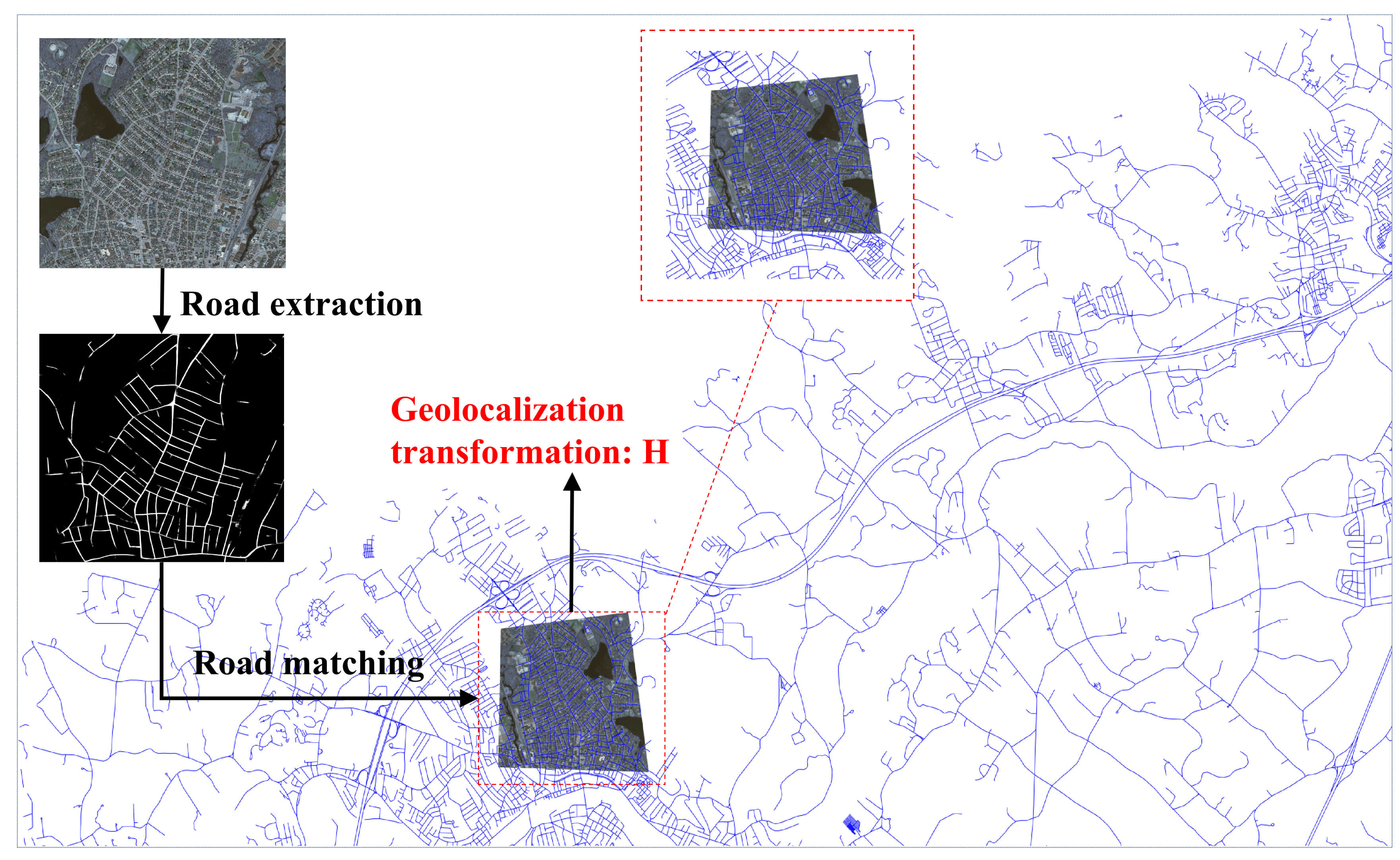
Aligning an aerial image to a known Geographical Coordinate System (GCS), which is called aerial image geolocalization, is a fundamental task in the field of remote sensing. Roads are a kind of salient feature on the ground and are labeled on the existing Geographic Information System (GIS), so we consider it feasible to align aerial images to a certain GCS with roads. As is shown in Figure 1, we develop an efficient geolocalization method imposed directly on the aerial images by registering the road networks in the aerial images to the reference road networks in the GIS when the approximate positions of the aerial images, i.e., in which city the aerial images are captured, are known. The proposed method can geolocalize an aerial image over a search area larger than 1000 km2 within seconds. Compared with traditional geolocalization methods, the proposed method is much less expensive and efficient, because the only sensor needed is the camera and the reference road vector map, which is highly compact and is readily available from many kinds of GISs (such as road vector maps from OpenStreetMap (https://www.openstreetmap.org)).
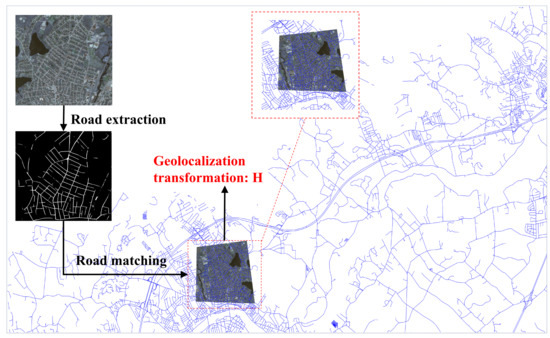
Figure 1.
The motivation of this study: performing efficient geolocalization directly on query aerial images by matching the roads in the aerial images with those in the reference road map (in blue) over an area as large as a whole city. Geolocalization is the task of estimating a transformation that aligns the aerial image to a certain Geographical Coordinate System (GCS). To make it clearly seen, only parts of the reference road map are shown here.
Though appealing, the task is quite demanding. The main challenges lie in the great appearance and geometric differences between the reference road vector map and roads extracted from the aerial images. On the one hand, despite the good performance of the state-of-the-art road extraction methods [1,2,3,4], much noise still exists, causing the extracted roads to be fragmented and incomplete; on the other hand, the reference road map may not be up-to-date, leading to some differences from the actual one. Such appearance differences make it difficult to measure the similarity robustly.
The geometric differences are mainly caused by the change of camera pose. Since the aerial images may be taken under any camera pose, it is necessary to use the 2D projective transformation to represent the mapping function between road points in the aerial images and the reference road vector map. Under the 2D projective transformation, most of the geometric features, including the lengths of line segments and the angles between two lines, are not invariant, leading to difficulties in establishing the correspondences between the roads in the aerial images and the reference road maps [5]. Because of this, many existing works on road based geolocalization [6,7,8,9] treat the transformation between the aerial image and the reference road network map as a similarity transformation, and extra attitude and altitude measurements from other sensors on the Unmanned Aerial Vehicles (UAVs) must be used to project the aerial images to the reference coordination.
Even though there are some shape matching methods [10,11,12] that can deal with the geometric deformation to some degree, they are not suitable for the task. The main drawback of these methods is that they can only deal with shape matching between two geometric primitive sets where the geometric primitives mostly correspond. In the geolocalization, the roads in the aerial images are only a small subset of the reference road maps, and it is hard to segment the corresponding part of the reference road vector map when the transformation is unknown. It is also inefficient to divide the reference road map into overlapping tiles and compare each tile with the roads in the aerial image with such shape matching methods because such tiles have difficulty capturing the correct corresponding area of the aerial image in the reference road map when the possible variation in translation, scale, and rotation is highly uncertain.
To address all the aforementioned challenges, we take a step further from our previous work [5] and develop a novel robust geolocalization algorithm. The core of the new method is a projective-invariant geometric feature, which consists of a road intersection together with all the road points surrounding it, called the Projective-Invariant Contour Feature (PICF) in this paper. The main motivation to design the PICF is that such a feature can split the same subsets of the point set under the 2D projective transformation, which can be proven mathematically. With such a property, we can encode the subsets of the point set in a projective-invariant manner. Compared with the “2-road-intersections-tuple” feature in [5], the PICF encodes much more geometric information and is more discriminative. This makes our algorithm more flexible. With much fewer initial feature correspondences and a much higher matching inlier ratio, each initial transformation recovered from the feature correspondences can be further refined with methods such as ICP [13,14,15]. Such a strategy eliminates the influence of the noisy estimation of the initial transformation, makes the geolocalization more robust, and improves the recall to a large extent.
Moreover, benefiting from the good invariance of the proposed PICF, a robust matching method, such as the methods proposed in [16,17,18], can be used to improve the matching quality further. Along with the PICF, we develop an effective matching algorithm considering the geometric coherence between matching pairs to improve the matching quality further. This is accomplished by minimizing the cost function, which includes the PICF descriptor loss and geometric inconsistency loss. The optimization problem can be solved sufficiently by employing the known graph cut method [18,19,20]. Finally, the correct transformation is determined by checking all the candidate matches. In this stage, a flexible way to recover the initial transformation from those correspondences is adopted. The homography transformation is estimated with all the correspondences when enough correspondences are found. Otherwise, we can recover the coarse transformation from just one matching pair and then refine it with a local-to-global ICP method. Such a strategy enables our method to deal with all cases efficiently no matter whether the roads in the scenes are dense or sparse.
2. Materials and Methods
2.1. Projective-Invariant Contour Feature
In this section, we first introduce the definition of the PICF and prove that the PICF is an equivariant representation under the 2D projective transformation group. Then, we introduce the details of the method to compute the PICF descriptor. Finally, we present a sufficient matching method, where the feature matching is modeled as an optimization problem to minimize both the matching distance between PICF descriptors and the geometric inconsistency between every two matching pairs.
2.1.1. Definition of the PICF
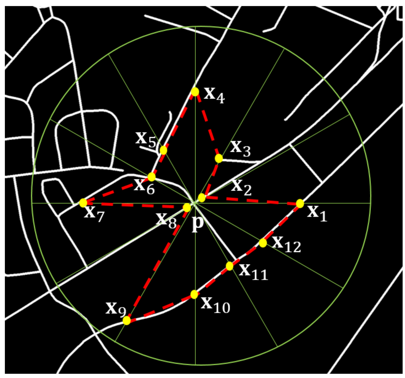
Given a set of 2D points and a 2D point , we then give the following definitions. All notations and definitions can be easily understood by referring to Figure 2.

Figure 2.
Definition of the Projective-Invariant Contour Feature (PICF). The contour of the point consists of all neighbor points in each direction. In this figure, we draw 12 neighbor points on the contour of in yellow and connect these points into a polyline in red. When more neighbor points are added, the polyline can approximate the contour of better. The PICF encodes the relative positions of points around .
Definition 1.
The neighbor point of in the direction of θ is the point , which meets the following conditions:
- (1)
- ;
- (2)
- , where is the angle of vector related to the X axis;
- (3)
- , if , then .
Definition 2.
The contour C of is the set of all the neighbor points of in point sets P: , where is the neighbor point of in the direction of θ.
2.1.2. Equivariance of the PICF
Equivariant representations are highly sought after as they encode both class and deformation information in a predictable way. Similar to the equivariance defined for the image in [21], the equivariance for the point set can be defined as follows:
Equivariance for the point set: Let G be a transformation group and be the group action applied to a point set P. A mapping is said to be equivariant to the group action , if:
where and correspond to the application of g to E and F, respectively, and satisfy .
In the case of the PICF, the mapping aims to extract the contour of a given point , and we will show that this mapping is equivariant to the 2D projective transformation group.
The equivariance of contour under the 2D projective transformation can be defined equally as follows:
Theorem 1.
Let be the point set after applying the 2D projective transformation H to P, be the corresponding point of , and be the contour of and , respectively, for any point ; there exists a point , which satisfies , and equally, for any point , there exists a point , which satisfies , where is the inverse transformation of H.
Before the proof of Theorem 1, we introduce another theorem.
Theorem 2.
Let l be the line passing through points , be another point on line l, and be the corresponding points of under the homography transformation H. can be computed with as , where:
Theorem 2 shows us the fact that the relative order of points on a line stays the same under the homography transformation. The proof of Theorem 2 is provided in Appendix A.
Proof of Theorem 1.
Let be the ordered points on the line in the point set P, where , if , and be the corresponding points of under the homography transformation H. As is illustrated by Proposition 2, are collinear, and if , which means is the point closest to in the direction of angle . Therefore, is a point on the contour of ; that is to say, there exists a corresponding point for any point , which satisfies . Since the homography transformation is reversible, for any point , there exists a point , which satisfies , where is the inverse transformation of H. □
2.1.3. The PICF Descriptor
At this point, we have introduced the definition of the PICF and proven its equivariance under the 2D projective transformation. Even though we know that the points on the contour correspond one-to-one, we still do not know the definite corresponding point of a certain point. Therefore, it is necessary to align the contour point sets to the same direction and scale in order to encode the corresponding PICFs with the same descriptors.
Let the local coordinate relative to point of a point on the contour of be and the local coordinate of its corresponding point under the 2D projective transformation be . Since the homography transformation projects point to , we can get:
Since the projective transformation can be approximated to the affinity transformation in most applications in remote sensing, which means is close to the zero vector, the transformation between and can be approximated as:
Equation (4) emphasizes an important fact that the transformation between the local coordinate and can be approximated as a linear transformation, which can be presented with a matrix. Since an undetermined matrix has 4 parameters and each point-to-point correspondence accounts for two constraints, it is necessary to specify 2 point correspondences in order to constrain the transformation fully.
Even though we cannot obtain the exact correspondences between two contour point sets, we know that they correspond one-to-one; that is to say, for a certain point , there exist a certain point that is corresponding to it, which satisfies . Adding all the points up, we get:
Let:
be the centroid of contour C and , respectively; we get:
The line l passing through the center point and the centroid of contour C divides the contour into two parts and , and similarly, the line passing through the center point and the centroid of contour divides the contour into two parts and . Since the points correspond one-to-one and the line l and also correspond, the points in should also correspond one-to-one to those in or . Similar to the definition of the centroid of the whole contour, we define the centroid of the half-contour as:
Then, there exist two possible correspondences: and . Therefore, we get two possible constraints or .
With the correspondences of the centroids of the contours and centroids of the half-contours, we get two groups of possible constraints,
with which the transformation matrix can be determined. The contours can be aligned to the same coordinate with the transformations so that we can get a projective-invariant description of the contour.
As is shown in Figure 3, the detailed method to compute the PICF descriptor is:

Figure 3.
Compute the PICF descriptor. (a) The contour point set is collected by finding the closest points in each direction interval; (b) the centroid of the whole contour and two centroids of the half-contours are calculated, which are shown in green and red, respectively; (c) the contour is aligned with two affinity transformations, respectively, which is estimated by aligning the centroid of the whole contour and the centroids of the half-contours to given points; the two aligned contours are shown in pink and yellow, respectively; (d) the two contours reconstructed from the PICF descriptors are shown in pink and yellow, respectively, and the original contour is shown in light blue.
- (1)
- Sample contour points: Divide the area centered at point into N areas with angle step ; for each area ; find the closest point to ; and take as the sample point on the contour in direction ; compute the relative coordinate of to point as ; if no point exists in the area, then set .
- (2)
- (3)
- Align contour points: Project all contour points with and , respectively, and get two transformed point sets and .
- (4)
- Compute the PICF descriptor: Convert the coordinates of the points in point sets to the polar coordinates, and sort the points with their angles in ascending order, then we get . For each area , compute the average distance of contour points in the area to the center point as: , where is the dimension of the descriptor, and ’. Finally, the two possible PICF descriptors of point in the point set P are obtained as: .
2.1.4. Discussion
As proven in Section 2.1.2, the equivariance of the PICF under the 2D projective transformation holds strictly true when the direction angle is continuous. To represent the contour point set with the vector, as introduced in Section 2.1.3, the contour point set is sampled with discrete . The strict equivariance does not hold in such a case, but the equivariance is approximately satisfied when the sample step is small enough. For each point on the contour, there exist points that are close enough to its corresponding point on the transformed contour as long as the sample step is small enough, which means the approximate corresponding point always exists. Therefore, in our implementation, the number of sample contour points is set to the dimension of the PICF descriptor to make the sample contour a better approximation of the full contour. Besides, we choose the closest points to the center in each small direction interval as the sample points of the contour, which makes the estimated PICF descriptors less sensitive to small breaks of the detected roads. These measures make approximate equivariance hold well in practical applications, which is also proven by our experiments.
2.2. Matching PICFs with Geometric Coherence
At this point, given a point set P and a center point , we can compute a projective-invariant descriptor, which encodes the local point cloud information. With such a descriptor, many fast retrieval algorithms, such as the FLANN [22], are sufficient to build the correspondences of two PICF sets. However, large amounts of outliers exist in the correspondences estimated from such methods, which leads to more unnecessary tries in the following transformation refining and validation. To solve the problem, we model the PICFs matching as an optimization problem to minimize the cost function, which penalizes the differences between the PICF descriptors and also the geometric inconsistency between two matching pairs.
2.2.1. Geometric Coherence between PICF Correspondences
Let be a matching PICF pair, where are the transformation matrices in computing the PICF descriptors of , respectively, and are the corresponding PICF descriptors. For a certain point and its corresponding point , the transformation between them is:
Multiply both sides of Equation (11) by ; we get . Let , then for all PICF correspondences, their corresponding are equal, as deduced in Section 2.1.3.
Considering the geometric consistency between matching pairs, the matching between two PICF sets and can be modeled as a problem to minimize the cost function:
where are the indexes of the corresponding PICF in of th and th PICF in , respectively. The first term of Equation (12) is the data term, which models the matching distance between PICF descriptors, and the second term is the smooth term, which penalizes the geometric inconsistency between two matching pairs.
2.2.2. Refining Initial Matches with Geometric Coherence
It is difficult to solve Equation (12) directly; instead, we seek a two-stage solution. We first find the best matching for each PICF and then verify the correctness of the correspondences with both the matching distances and geometric consistency, as described in Section 2.2.1.
Let be the initial correspondences found with descriptors matching, be the matching distance of , and be the corresponding transformation matrix of . We define a label function , which maps to 1 if the matching is correct, and 0 otherwise. Then, the PICF matching problem is equivalent to finding the labels of all initial correspondences that minimize both the matching distances and geometric inconsistency.
where , are the kernel functions. We use the kernel function to normalize both the data term (matching distances) and the smooth term (geometric inconsistency) to improve the robustness. is the distance between and and is calculated with the method proposed in [23].
The data term is defined as:
This energy term penalizes matching pairs whose labels are 1, but with large matching distances, and those whose labels are 0, but with small matching distances.
The smooth term is defined as:
In , if both correspondences are labeled as outliers, the penalty is , thus “rewarding” label 0 if the geometric inconsistency is big. The penalty of considering a pair of correspondences as the inlier is , which rewards the labels if the transformation matrices of the two correspondences are similar.
Equation (13) can be solved efficiently and globally via the graph-cut algorithm [18,19,20]. The complete matching algorithm considering geometric consistency is illustrated in Algorithm 1.
| Algorithm 1 PICF matching algorithm. |
|
2.3. PICF Based Fast Geolocalization
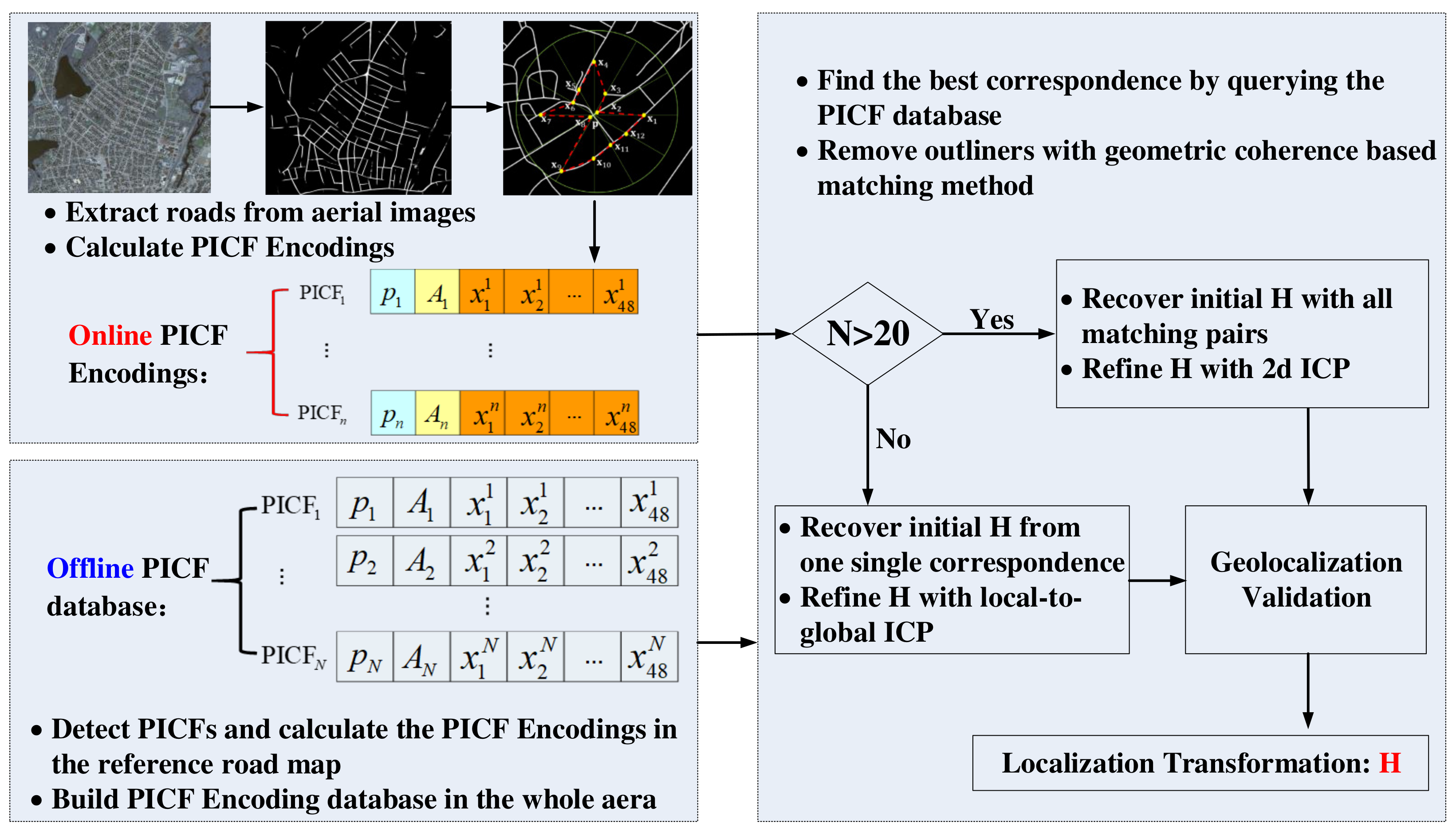
At this point, we propose the PICF, which is equivariant to the homography transformation group, and a way to describe the PICF by a vector invariant to homography transformation, with which the potential correspondences can be found effectively. Furthermore, to improve the matching, we model the PICFs matching as an optimization problem to minimize the cost function, which penalizes the differences between PICF descriptors and also the geometric inconsistency between two matching pairs, and solve it with the graph-cut algorithm sufficiently. In this section, we introduce our fast geolocalization method based on the PICF in detail. The overview of our method is shown in Figure 4.

Figure 4.
Overview of the proposed PICF based geolocalization method. Compared with the method in [5], the newly proposed algorithm is more sufficient, which is mainly a benefit of the good performance of the newly-designed PICF. The performance improvements come from two aspects: on the one hand, the effective encoding of the road geometric structure by the PICF, together with the effective matching method considering geometric coherence between correspondences, leads to an initial correspondences set with a high inlier ratio; on the other hand, benefiting from the good matching results (only at most one matching candidate for each feature), each recovered homography transformation can be refined, making it more robust and less sensitive to initial transformation estimation to verify whether the geolocalization is correct. Here, N is the number of obtained matching pairs.
Our fast geolocalization method contains the offline stage and the online stage. The offline stage is for processing the reference road vector map whose output is used in the online correspondence search scheme, allowing for a very fast operation. As is illustrated in Figure 4, in the offline stage, all the road intersections are detected and used as the centers of the PICFs; and then, the two possible PICF descriptors are computed for each PICF; finally, a KD-tree is built using all these PICF descriptors.
The proposed online search scheme starts by extracting the roads for a given aerial image using our method in [1]. The same as the offline stage, all the PICFs are detected, and their corresponding descriptors are calculated. The correspondences between the query PICF set and the reference PICF set are found with the geometric-consistent matching algorithm introduced in Section 2.2. These matching PICF pairs are then used to recover the homography transformations between the aerial images and reference road map with two different strategies:
- (1)
- If the number of matching pairs is larger than (20 in this paper), an initial homography transformation is estimated with all the matching pairs using the RANSAC method and then refined with the plain ICP. The refined transformation is then verified with the alignment accuracy between the query road map and the reference road map.
- (2)
- If the obtained feature correspondences are less than or the first strategy fails to recover the right transformation, the obtained pairs are afterward sorted with their matching scores. Then, a homography transformation is estimated with a single correspondence and refined using all the road points in the query road map with a local-to-global iterative closest point algorithm. Furthermore, the refined transformation is then verified with the alignment accuracy. Each correspondence in the sorted pair set will be tested until a homography transformation that aligns the query road map and the reference one accurately enough is found. If our method fails to recover the correct transformation after all the correspondences obtained with the geometric-consistent matching algorithm, the left correspondences in the initial matching will be checked in the same manner.
2.3.1. Initial Homography Transformation Estimation from One Matching Pair
Give a PICF correspondence , the coarse homography transformation , which projects the query road point to the reference road point, can be computed as:
- (1)
- Compute matrix : ;
- (2)
- Compute vector : the homography transformation is approximated to a affinity, so we get ;
- (3)
- Compute the translation vector : since the contour center point is projected to , we get .
2.3.2. Transformation Refining
When the approximate homography transformation is estimated from a given correct PICF correspondence, the estimated homography transformation has poor accuracy and should be refined further. This is because is approximated to an affinity transformation, and the upper-left matrix is estimated using only points on the contour.
The initial transformation estimated from one correspondence is refined so that it aligns the query road point set to the reference road point set accurately. The ICP algorithm is appropriate to solve such a problem. However, in our experiments, we find that the convergence rate is quite low when using the plain ICP algorithm, which may arise from the poor accuracy of the initial transformation. Since the initial transformation is estimated with the points near the center point of the PICF, it should be accurate enough for points near the center point. Inspired by [15], we use a local-to-global ICP algorithm, which first aligns the points near the center point and then aligns the points far from the center point gradually.
In the local-to-global ICP algorithm, the points whose distances to the center point are less than d in the query road point set are chosen to refine the initial transformation with the standard ICP algorithm firstly. If the ICP algorithm is convergent, the refined transformation is then used to align the points whose distances to the center point are less than , resulting in a further refined transformation ; otherwise, the correspondence used to estimate the initial transformation is regarded as an incorrect correspondence and is discarded. The optimization continues until all query road points are used.
2.3.3. Transformation Validation
After the transformation refining, the homography transformation estimated from a correct correspondence aligns the query road point set with the reference point set accurately, while the homography transformation estimated from an incorrect correspondence cannot. We use the inlier rate of road points in the query road map to measure the alignment accuracy. A road point is regarded as an inlier when the distance between its projection point under estimated transformation and the closest road point in the reference road map to its projection point is less than a certain threshold . Therefore, the inlier rate can be computed as:
where is the projection point of under .
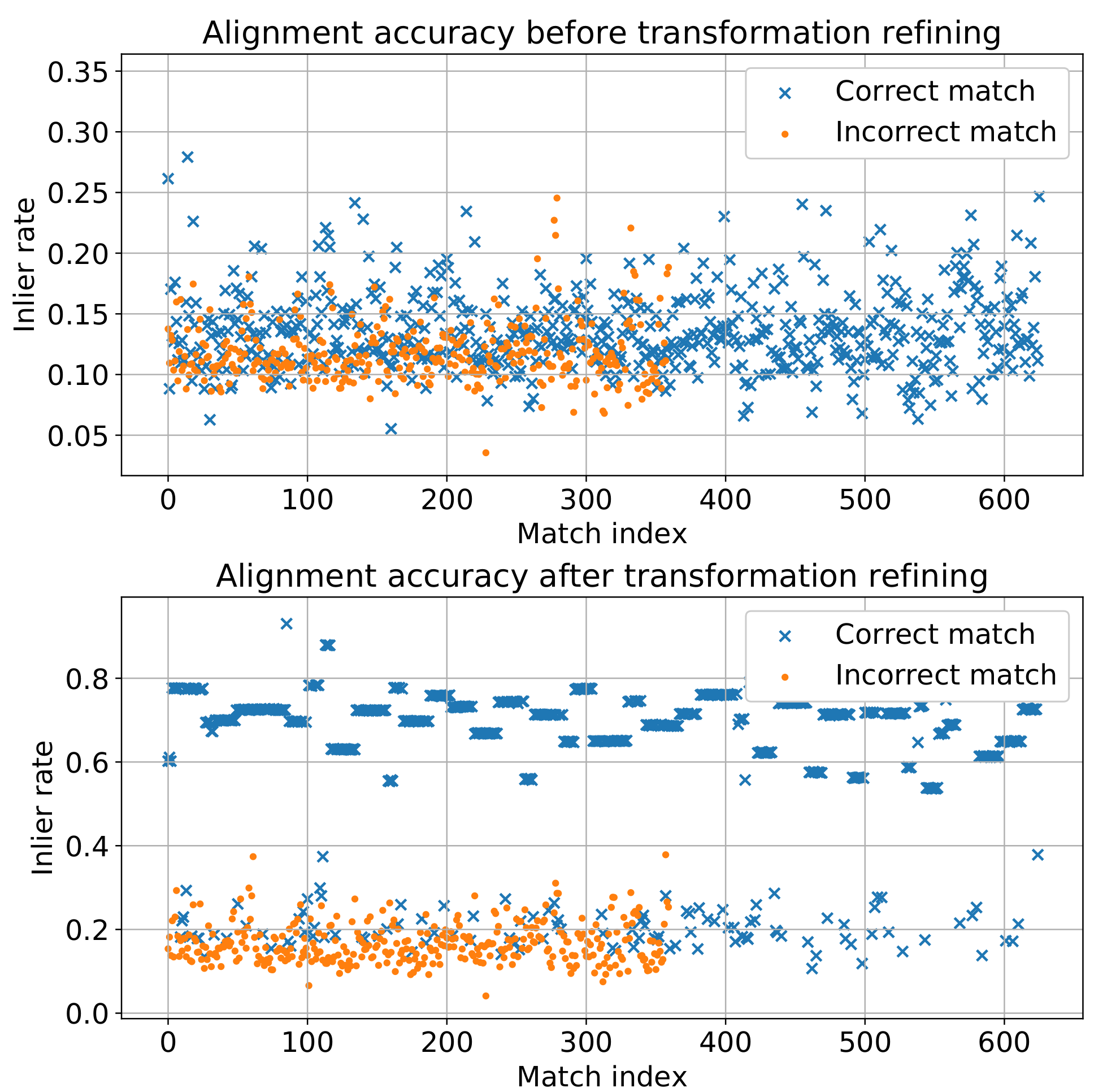
One may argue that the transformation validation should be done with the initial transformations estimated from the correspondences before the transformation refining to remove incorrect correspondences further and to reduce unnecessary tries to find the correct transformation. However, in our experiments, we find that the inlier ratios under the coarse transformations are not sufficient to distinguish the right transformations from those that are wrong. As is shown in Figure 5, before the transformation refining, the inlier ratios are low under both the transformations estimated from the correct and incorrect correspondences, and there is not an obvious threshold of inlier ratio that can distinguish the correct transformations from these wrong ones. After the transformation refining, the inlier ratios of correct transformations are much higher than those of incorrect transformations in most of the cases.
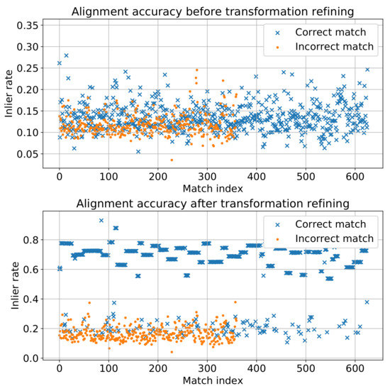
Figure 5.
Alignment accuracy before and after transformation refining. Before the transformation refining, neither the transformation estimated from a correct match, nor that from an incorrect match can align the query road point set to the reference road point set accurately. After the transformation refining, the alignment accuracy under most of the transformations estimated from the correct matches improves greatly, while that of the incorrect match does not.
3. Results
In this section, we firstly perform experiments on large-scale synthetic aerial image data sets to evaluate both the effectiveness of the PICF and the geolocalization method. Then, experiments on real aerial image data sets are conducted to test the performance of our algorithm on real applications.
Implementation details: Our implementation was written in C++, single-threaded. All the experiments ran on a computer with an Intel Xeon E5-2620v2 CPU and 24 GB RAM. In all the experiments, the road maps for aerial images were extracted with our road segmentation method proposed in [1] in advance. The parameters of our algorithm were set based on experiments on a validation synthetic aerial image data set and kept fixed in all experiments. The main parameters settings were: the dimension of the PICF descriptor ; the weight for smooth energy term , where N is the number of initial correspondences; the parameters of the kernel function for the data term and smooth term and , respectively; the maximum iterations for plain ICP ; the distance to divide the query road points into different parts in local-to-global ICP , where are the width and height of the query road image, respectively; the ratio of the distance to expand the points to align in local-to-global ICP ; the distance error threshold for a road point to be regarded as an inlier ; the minimum required inlier ratio to verify the geolocalization as correct .
Baseline and metrics: We compared our method with the state-of-the-art algorithm, the “2-road-intersections-tuple” (2RIT) based geolocalization method [5], in three aspects: precision, recall, and run time. Here, , where is the number of successfully and correctly geolocalized aerial images and is the number of successfully, but wrongly geolocalized aerial images; , where N is the number of all aerial images used. We used the error between the estimated homography and the ground truth one to verify whether the geolocalization was correct, which is computed with the same method as in [5]. In all experiments, the parameters for “2RIT” were set the same as reported in [5].
3.1. Experiments on Synthetic Aerial Image Data Sets
In this section, experiments on synthetic aerial image data sets are conducted to test the performance of our geolocalization method under different viewing angles, resolutions, and scenes. Since it is quite difficult to collect enough aerial images with the needed viewing angles, resolutions, and context, we followed the same manner as in [5] to validate our algorithm using synthetic aerial image data sets. The three reported synthetic aerial image data sets in [5], named “multi-poses data set”, “multi-GSDs data set”, and “multi-areas data set”, were used in our experiments to test the performance of our method under different viewing angles, resolutions, and scenes, respectively. Each data set contains synthetic aerial images from two different areas in Massachusetts. The roads in one area (the 13th area) are sparse, while roads in the other area (the 17th area) are much denser. Therefore, these data sets are representative.
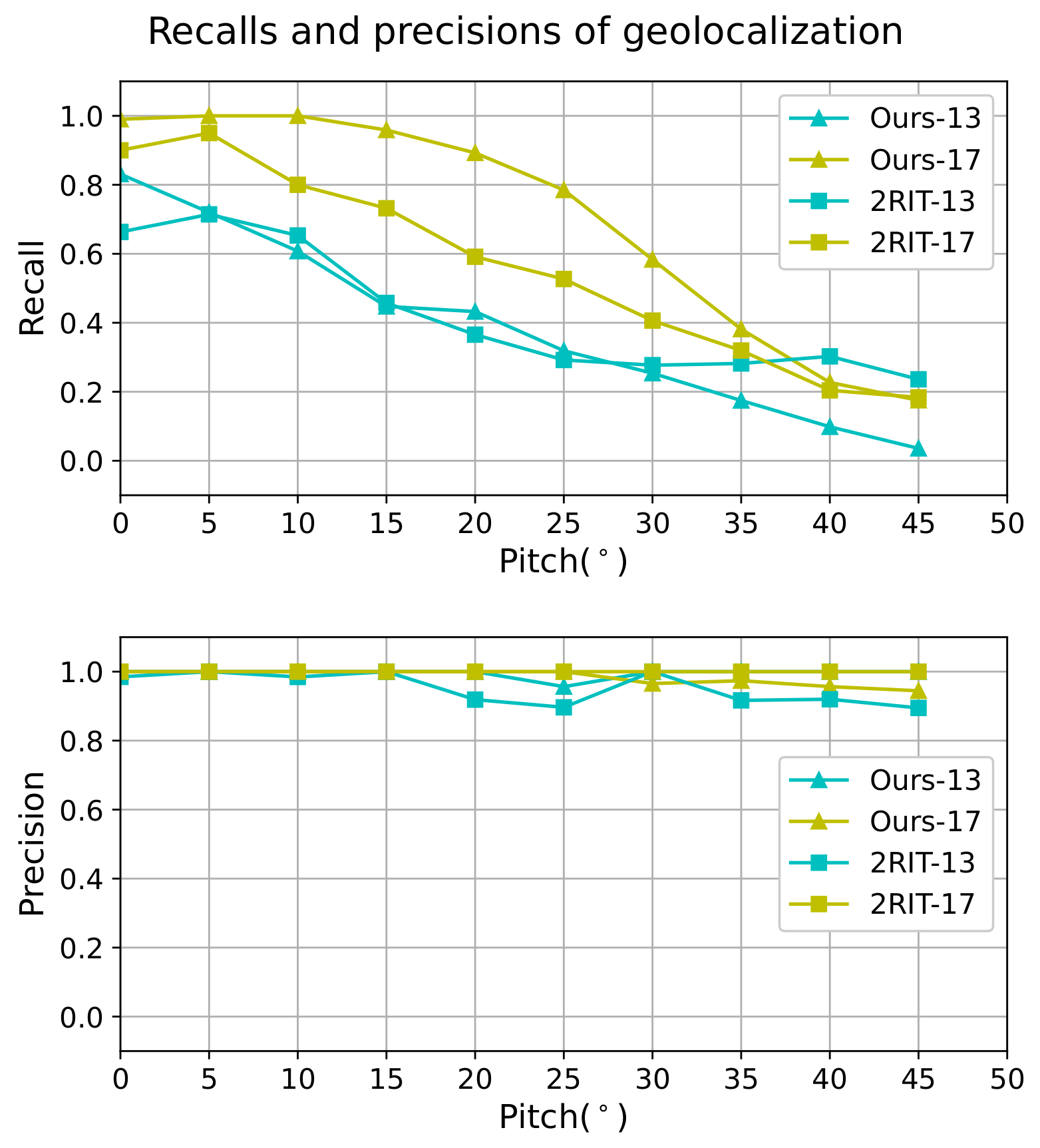
As is shown in Figure 6, the precision of the two methods in both areas is higher than for all aerial images taken under different viewing angles. Meanwhile, our novel method improves the recall in both areas when the viewing angle is less than , which is usually the case in real applications. The improvement of recall is especially significant in the 17th area where the roads are dense. Figure 6 also shows that the recall of both methods decreases with the increase of the viewing angle. However, the performance degradation of the method presented in this paper is much slower.
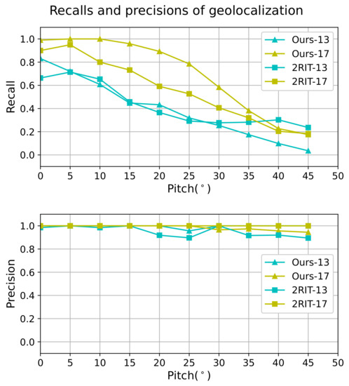
Figure 6.
Precision and recall of geolocalization under different viewing angles of the “2-road-intersections-tuple” (2RIT) method [5] and our method.
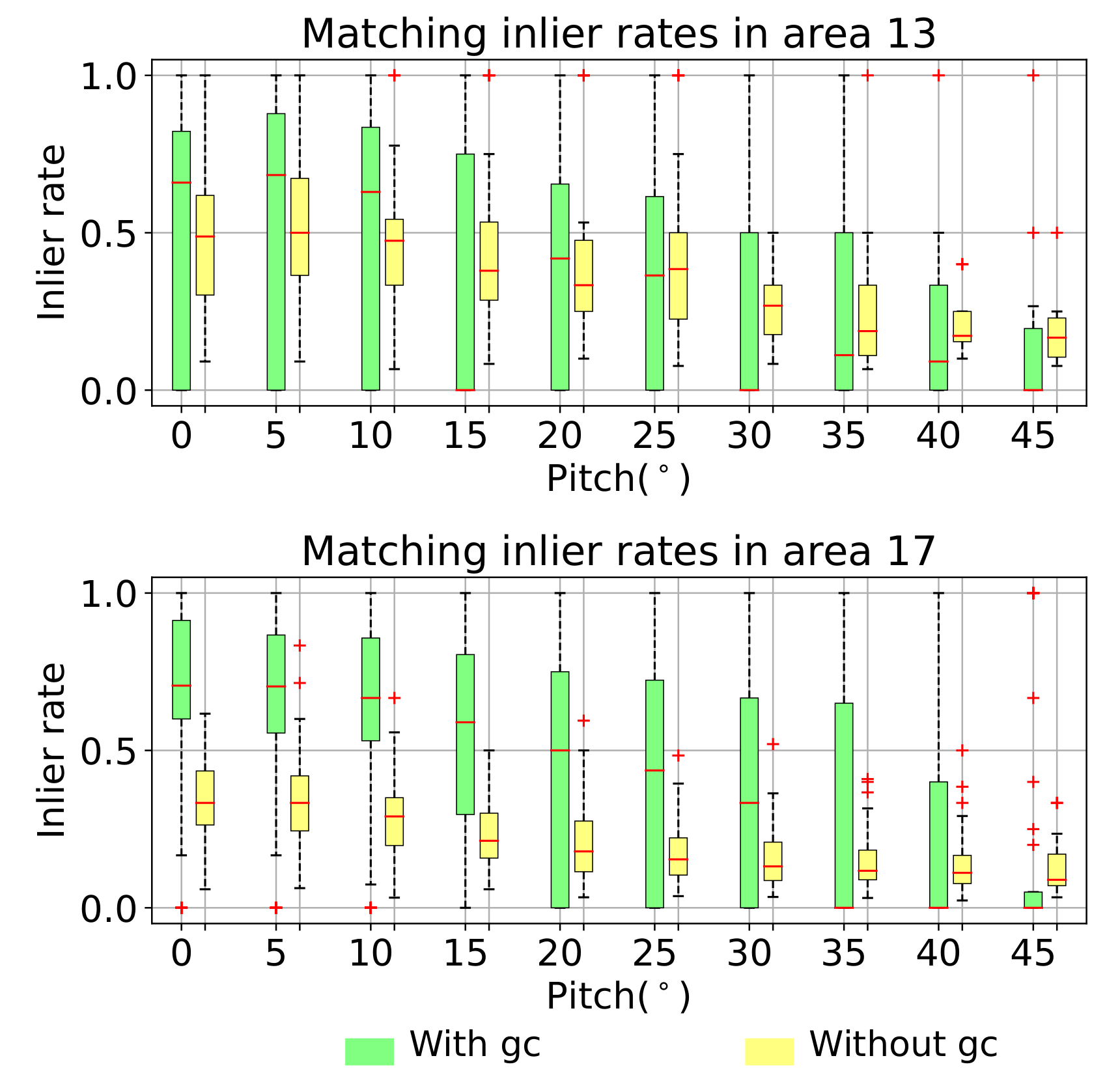
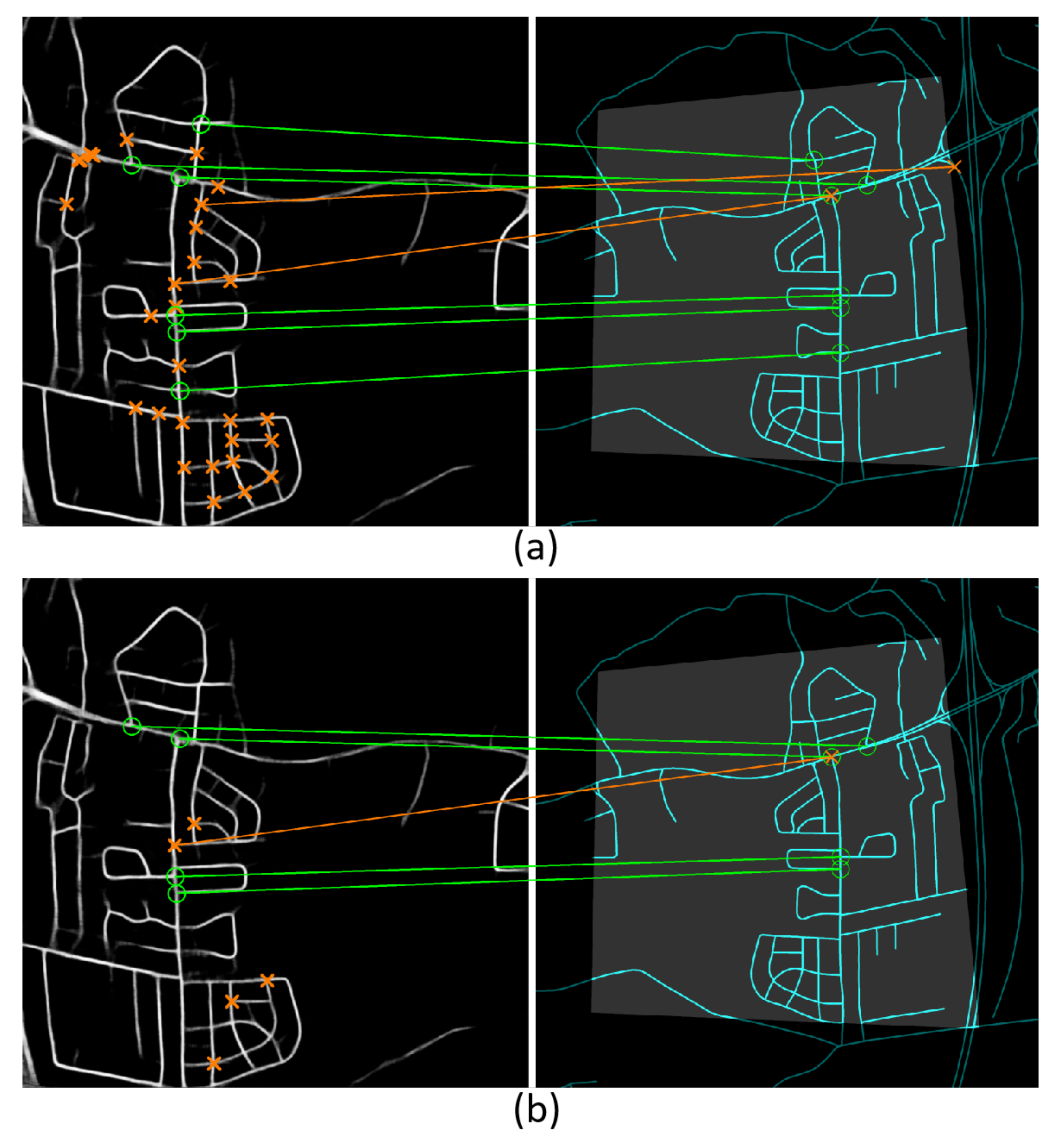
Figure 7 shows the matching inlier rates under different viewing angles in both areas. As can be seen, the inlier rate of the initial PICF correspondence set obtained with finding the nearest neighbor in the PICF descriptor space is acceptable. In both areas and under all view angles, the inlier rate of the initial correspondence set is no less than , which indicates that the proposed PICF can encode the geometric structure effectively and is discriminative. It also proves that the PICF is projective-invariant. Furthermore, the geometric coherence based matching method is efficient to improve the initial matching quality, especially when the viewing angle is relatively small. As is shown in Figure 8, the improvement mainly comes from the ability of the geometric coherence based matching method to reject most of the wrong correspondences while preserving most of the right correspondences. The good performance is more obvious when the roads are dense in the search area (17th area). In such areas, the similar local structures of the road network are ubiquitous, leading to a low inlier ratio of initial matching. It is thus more meaningful to use the geometric coherence constraint. The improvement of the matching inlier rate is significant to reduce the unnecessary tries in the following geometric consistency validation and to improve the efficiency. Even though the geometric coherence based matching method is less effective when the viewing angle is large, since it may reject all the right matching pairs for some aerial images in such a case, leading to an inlier rate of zero, we try to recover the homography transformation from the rest candidates to ensure our algorithm can work in such a case.
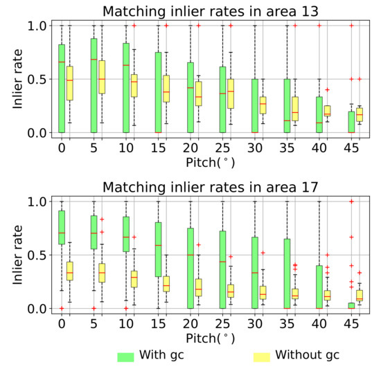
Figure 7.
Inlier rates of correspondences for each aerial image before (without gc) and after (with gc) graph-cut optimization under different viewing angles.

Figure 8.
Matching result of the PICF for one road map before (a) and after (b) graph-cut optimization. The query road map is projected onto the reference road map with a padding of 200 m, and the projection areas are highlighted in gray. The projection images (right) are resized to the same height as the query road images (left). The correctly matched PICFs are marked with green circles, while those incorrectly matched are marked with orange crosses. The correct correspondences are shown in green, while the incorrect correspondences are shown in orange. The incorrect correspondences whose PICF centers in the reference road map fall out of the projection area are not shown with lines.
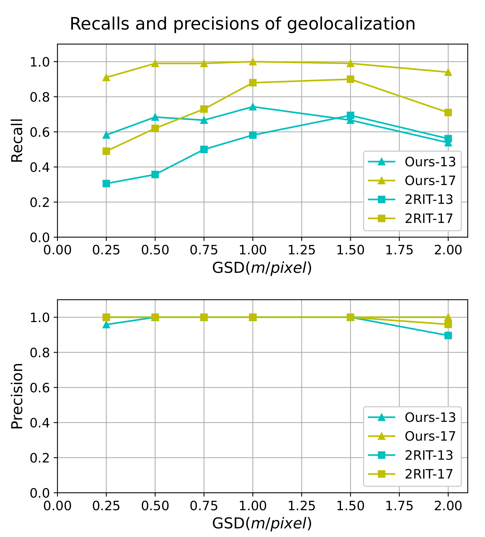
We also conducted experiments on the “multi-GSDs data set” to evaluate the influence of Ground Sample Distance (GSD) on the geolocalization. The result is shown in Figure 9. It can be seen that the recall of the “2RIT” method decreases sharply when the aerial images are captured with small GSDs, which indicates that the “2RIT” is sensitive to the GSD. Our PICF based geolocalization method is less sensitive to the change of GSD since the recall varies much more slightly with the GSD compared with the “2RIT” method.
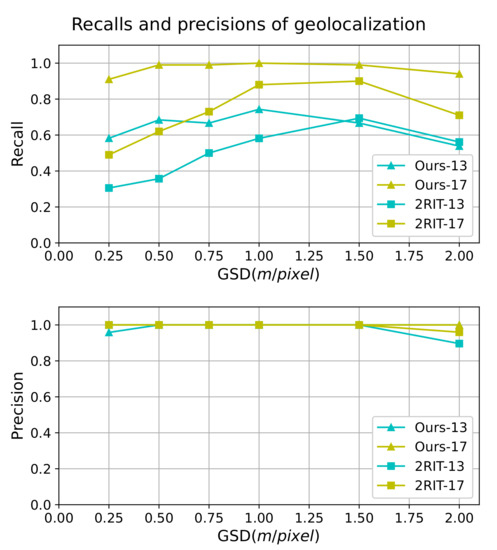
Figure 9.
Precision and recall of geolocalization under different GSDs of the “2RIT” method [5] and our method.
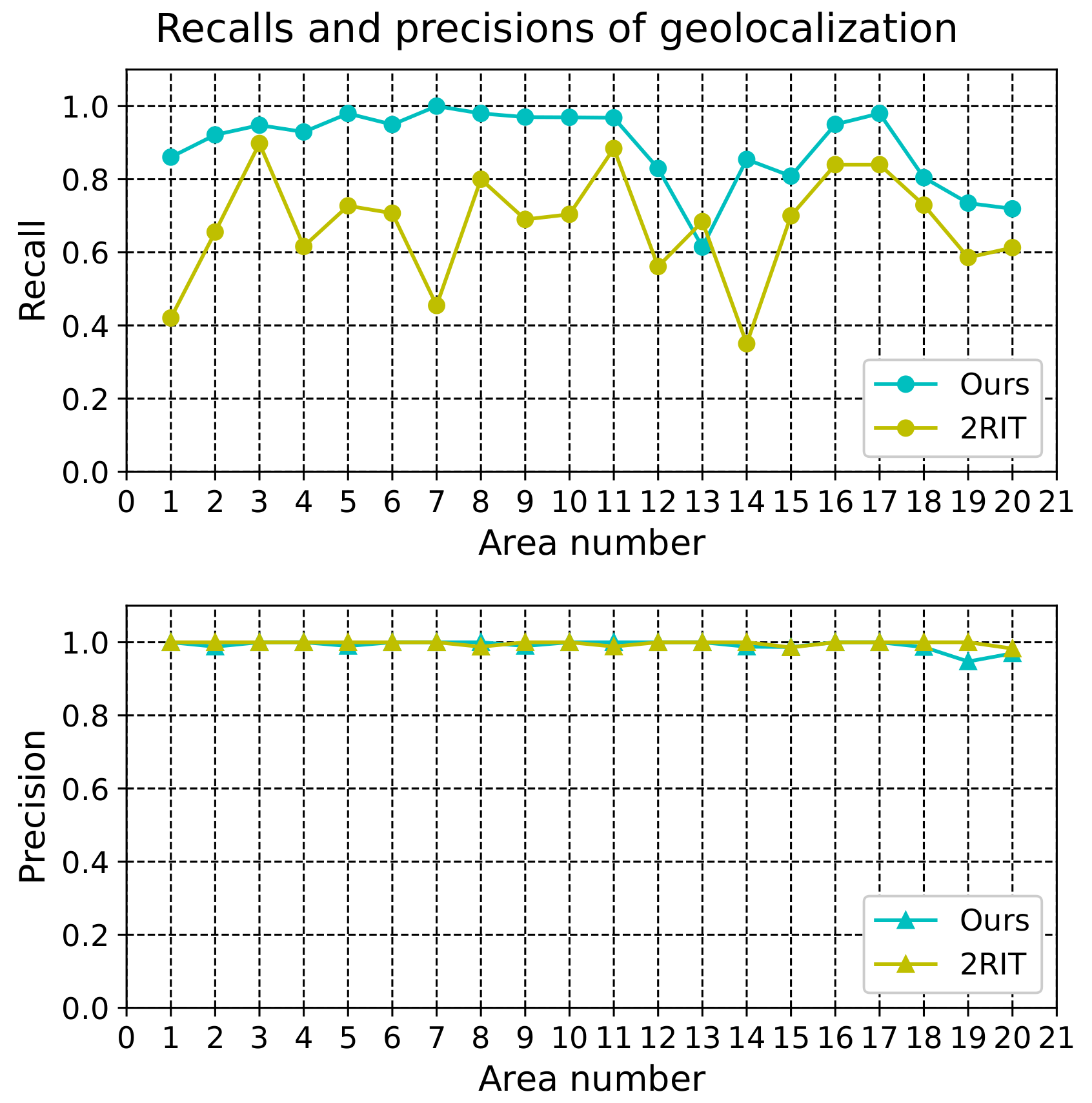
To study the performance of our method on different scenes, we conducted experiments on the “multi-areas data set”, which contains as many as 2000 aerial images from 20 areas. The precision and recall are shown in Figure 10. As can be seen, in all 20 areas, the precision of both methods is higher than . The recall of our newly proposed method is improved significantly in 19 out of 20 areas. In 12 areas, the recall is higher than . We highlight the improvement of recall in the first and seventh area. Several big cities lie in these two areas, leading to very dense roads. The similar structures of the road network in these two areas are ubiquitous. In such a case, the “2RIT” method may fail, since there exist too many candidates for each “2-road-intersections-tuple”, while our new algorithm performs well in such case. When a large amount of matching PICF pairs is found, it is robust and accurate enough to estimate the initial homography transformation using all these pairs. Such a strategy makes our algorithm effective at dealing with such cases. The only area where the recall of the new method is less than the “2RIT” method is the 13th area, and this is mainly caused by the too sparse roads in some aerial images, leading to few PICFs found in those aerial images.
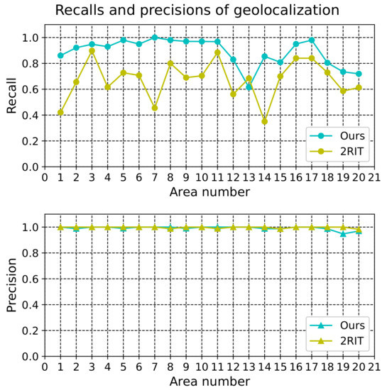
Figure 10.
Precision and recall of geolocalization in different areas of the “2RIT” method [5] and our method.
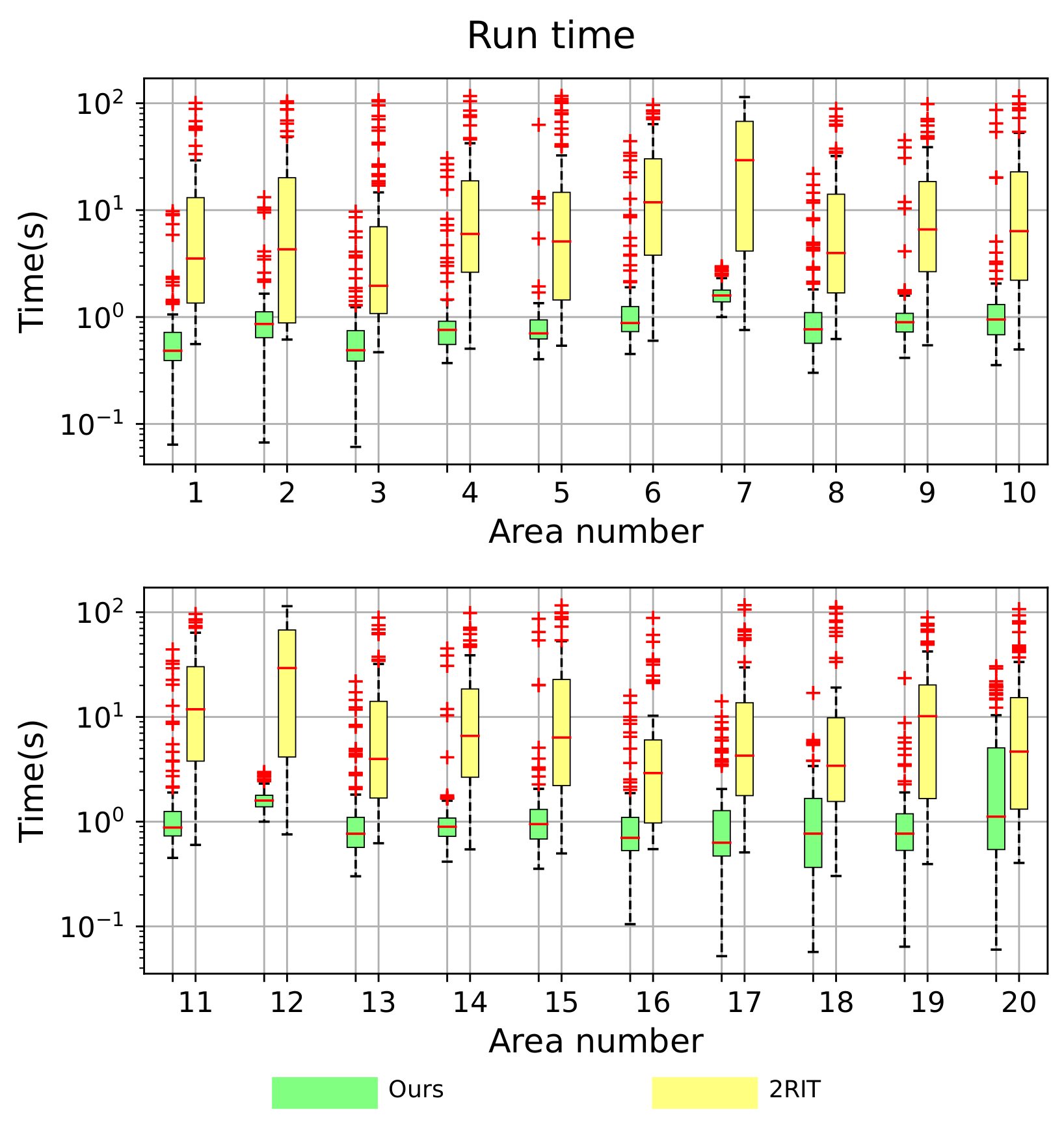
The run time of geolocalization for both methods is shown in Figure 11. In 17 out 20 areas, the average geolocalization time method proposed in this paper is less than 1 s and is less than 2 s in all 20 areas, while the average run time for “2RIT” is usually several seconds or even tens of seconds in areas like the seventh area and the 12th area. In all areas, the average run time of our new algorithm is less than that of “2RIT”. Besides, the run time of the PICF based geolocalization method varies more slightly between different aerial images in the same area compared with “2RIT”.

Figure 11.
Run time of geolocalization on the “multi-areas data set”. Here, run time refers to the time usage in the querying stage, which includes the time for PICF detection and descriptor computing, the time for PICF matching, and the time for estimating, refining, and validating the transformation.
3.2. Experiments on Real Aerial Image Data Sets
We also conducted experiments on real aerial images captured with cameras on UAVs to test the performance of our algorithm in real applications. We collected aerial images from three areas over China, including Suizhou, Xian, and Fengyang. The aerial images were captured in the form of videos. The details of the videos are shown in Table 1. These videos were then downsampled with one frame every 48 frames. All the selected aerial images in Suizhou were then resized to the resolution of , and aerial images in the other two areas were resized to , while the final GSDs of those aerial images ranged from 0.3 m/pixel to 1.0 m/pixel. The camera internal parameters were calibrated, and the distortion of the images was corrected offline.

Table 1.
Details of the real flight aerial image data set.
Since the Field Of Vision (FOV) of the camera is less than , the observed ground area in one single aerial image cannot cover enough roads. The roads in individual aerial images are not enough to determine their positions uniquely. Therefore, we stitched the aerial image sequences into bigger aerial mosaics to ensure that each mosaic contained enough roads. The final mosaics covered an area of 0.5 km2 to 3.0 km2. Finally, we obtained 21, 24 and 7 aerial image mosaics in Suizhou, Xian, and Fengyang, respectively. We then performed road segmentation to generate the corresponding road images for each mosaic, and those road images were then used to perform geolocalization.
All the reference road maps used in the geolocalization were downloaded from the Gaode map website (https://wprd01.is.autonavi.com/appmaptile?x=x&y=y&z=z&lang=zh_cn&size=1&scl=2&style=8<ype=11) with QGIS, which were saved in the raster map format with the resolution of 1.0 m/pixel. Each reference road map was large enough to cover the area where the aerial images were captured. The detailed information for the reference maps is shown in Table 2.

Table 2.
Details of reference road map for each area. The longitude and latitude are measured under WGS 84.
We conducted geolocalization on the generated road images with both the “2RIT” method and our new method. Since the ground truth of homography transformation between the aerial image mosaics and the reference road map cannot be obtained, we verified whether the geolocalization is correct by projecting the aerial images onto the reference road map and checking visually whether they overlap with the reference road map well. The result is shown in Table 3.

Table 3.
Geolocalization result on the real flight aerial image data set.
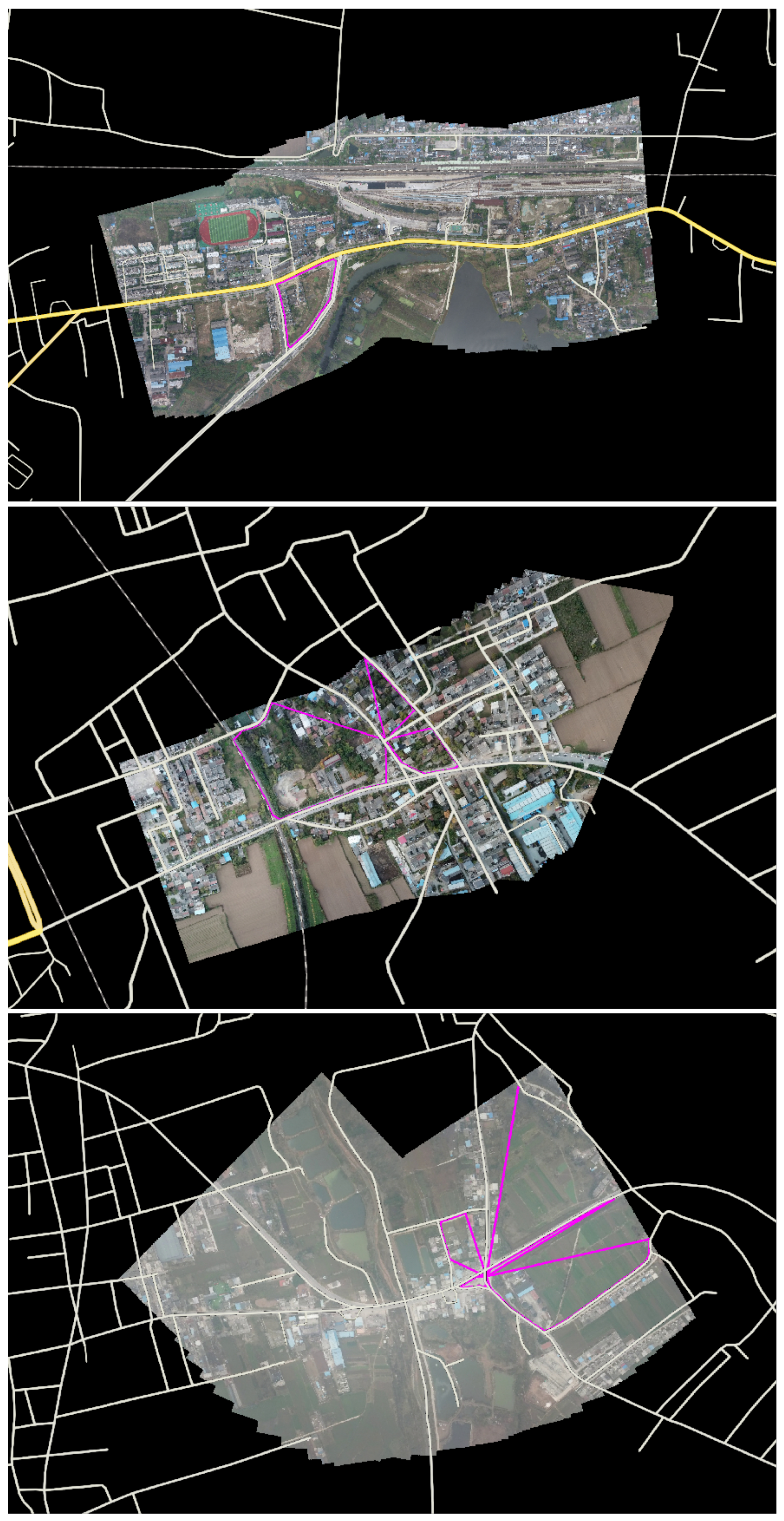
In all three areas, the proposed method outperformed the “2RIT”. The improvement is especially significant in Xian and Fengyang, where the recall increased by 42.86% and 28.57%, respectively. Compared with those in Suizhou, the GSDs of the mosaics in the two areas were higher. The width of roads may be more than 40 pixels in the road images for the main streets, making it difficult to estimate the tangents accurately. In such cases, the “2RIT” method failed. Our newly designed PICF is insensitive to road width, as is shown in the experiments on the synthetic data sets, which makes our new method more robust. Some cases where the “2RIT” failed while the proposed method succeeded are shown in Figure 12. The proposed method failed when no complete PICF was found in the scene. The PICF becomes less valuable when there exist too many directions in which no contour point is found, leading to the failure of geolocalization. A camera with a larger FOV may overcome this deficiency, which is left for further validation in our future work.

Figure 12.
Successful geolocalization results. The query aerial image mosaics are projected onto the reference road maps. The PICFs from which the homography transformations are estimated are shown in purple. The top mosaic is from Fengyang, while the other two mosaics are from Xian. Even though the roads in the aerial images cannot be aligned to those in the reference road map exactly in some cases, the geolocalization results can be used as a good initial estimation to calculate more accurate transformation. However, this is not the target of this paper.
4. Discussion
The results of the experiments on both synthetic and real aerial image datasets show that our newly proposed PICF based geolocalization method improves the recall and run time to a large extent compared with the state-of-the-art “2RIT” method. Furthermore, the results indicate that the PICF based geolocalization method is more robust to differences of viewing angle and GSD between the aerial images and the reference road map. In this section, we discuss the main factors that contribute to these improvements in detail.
The improvement of recall mainly comes from two aspects. First, the proposed PICF is projective-invariant and encoded with a projective-invariant descriptor, which means the representation of the PICF is robust to viewing angle change. Moreover, the PICF can encode much more geometric information of the road network compared with the “2-road-intersections-tuple”, making it more efficient to establish initial correspondences, which can be clearly seen from Figure 7. Since few outliers exist in initial correspondences, it is possible to use time-consuming optimization methods, such as the ICP, to refine each estimated initial homography transformation in an acceptable run time. With more accurate homography transformation, the geometric consistency check is much more efficient, as is discussed in Figure 5. In the “2RIT”, there usually exist hundreds or even thousands of matching candidates, making it unreasonable to refine each hypothesis generated by the feature correspondences. Therefore, the “2RIT” depends heavily on the accuracy of the initial homography transformation estimation. A correct, but less precise hypothesis may be rejected wrongly when the estimation of the tangents of road branches is noisy. The other factor contributing to the improvement lies in the effectiveness of the proposed homography transformation refining strategy, especially the idea of recovering the initial homography transformation from just one matching pair and refining it with the local-to-global ICP method. Such a strategy makes our method feasible in more cases, even when the roads are sparse or the cover areas of the aerial images are relatively small.
The greater robustness of our new algorithm to changes of viewing angle and GSD also benefit from the good performance of the proposed PICF. On the one hand, the invariance of the PICF is proven mathematically. Therefore, the encoding of the PICF is robust to changes in viewing angle. On the other hand, no accurate geometric information, such as the tangent, is needed in the computing of the descriptor of the PICF, which makes the PICF descriptor less sensitive to road segmentation noise. In the “2RIT” method, the tangents of road branches are required to estimate precisely, which is hard when the road segmentation is not smooth or the GSD of the aerial image is small. Since when the GSD is small, the width of the road is usually dozens of pixels in aerial images, making it difficult to extract the centerlines of roads accurately. In such a case, the initial transformation is noise and may be rejected wrongly even when the correspondence between the “2-road-intersections-tuple” is correct.
Three factors contribute to the improvement of the efficiency. First, the PICF encodes more geometric information of roads and is more discriminative, leading to much fewer matching candidates. Second, the geometric coherence based matching method rejects most of the incorrect correspondences and improves the matching quality further. Last, the strategy of using all the matching pairs or only one matching pair to recover the initial transformation is elastic to deal with all cases despite the density of roads, making our method quite efficient to find the right location.
5. Conclusions
This paper presents an aerial image geolocalization method, which uses only the road vector map as the reference. The new method is capable of efficiently and effectively estimating the transformation aligning the query roads to the reference roads over a whole city within several seconds on a single CPU, making it possibly available in real scenarios. Experiments on both the synthetic and real aerial images show that our method can significantly improve the recall of geolocalization while maintaining high precision and efficiency compared with the state-of-the-art aerial image geolocalization methods based on road network matching. The experiments also highlight areas of potential improvement. In future work, we will further enhance the capability and useful ranges of our method by reducing its dependence on initial transformation estimations, especially on aerial images with few roads.
Author Contributions
Conceptualization, Y.L. and S.W.; methodology, Y.L. and D.Y.; software, Y.L. and H.H.; validation, Y.L, H.H. and D.M.; formal analysis, Y.L.; investigation, Y.L. and D.Y.; resources, D.Y.; data curation, Y.L. and H.H.; writing, original draft preparation, Y.L.; writing, review and editing, Y.L.; visualization, Y.L.; supervision, D.Y. and D.M.; project administration, S.W. and D.Y.; funding acquisition, D.Y. All authors read and agreed to the published version of the manuscript.
Funding
This paper is supported by the National Natural Science Foundation of China (Grant Nos. 61673017, 61403398) and the Natural Science Foundation of Shaanxi Province (Grant Nos. 2017JM6077, 2018ZDXM-GY-039).
Data Availability Statement
The data presented in this study are available in article.
Conflicts of Interest
The authors declare no conflict of interest.
Appendix A
Proof of Theorem 2.
Let be the transformation matrix of homography transformation H. Since H projects the point to point , we get:
Express with and ; we get:
Since H projects the points to , we get:
Let the coefficient of Equation (A4) be ; we get:
Therefore, can be computed as the linear combination of and as:
Compute the derivative of to as:
Since are known constants, changes monotonically with . Compute the values of at point with Equation (A5),
Since , increases monotonically with . Finally, we get:
□
References
- He, H.; Yang, D.; Wang, S.; Wang, S.; Li, Y. Road Extraction by Using Atrous Spatial Pyramid Pooling Integrated Encoder-Decoder Network and Structural Similarity Loss. Remote Sens. 2019, 11, 1015. [Google Scholar] [CrossRef]
- Batra, A.; Singh, S.; Pang, G.; Basu, S.; Jawahar, C.; Paluri, M. Improved road connectivity by joint learning of orientation and segmentation. In Proceedings of the IEEE Conference on Computer Vision and Pattern Recognition (IEEE), Seoul, Korea, 27 October–2 November 2019; pp. 10385–10393. [Google Scholar]
- Bastani, F.; He, S.; Abbar, S.; Alizadeh, M.; Balakrishnan, H.; Chawla, S.; Madden, S.; DeWitt, D. Roadtracer: Automatic extraction of road networks from aerial images. In Proceedings of the IEEE Conference on Computer Vision and Pattern Recognition (IEEE), Salt Lake City, UT, USA, 18–22 June 2018; pp. 4720–4728. [Google Scholar]
- Cheng, G.; Wang, Y.; Xu, S.; Wang, H.; Xiang, S.; Pan, C. Automatic road detection and centerline extraction via cascaded end-to-end convolutional neural network. IEEE Trans. Geosci. Remote Sens. 2017, 55, 3322–3337. [Google Scholar] [CrossRef]
- Li, Y.; Yang, D.; Wang, S.; He, H.; Hu, J.; Liu, H. Road-Network-Based Fast Geolocalization. IEEE Trans. Geosci. Remote Sens. 2020, 1–12. [Google Scholar] [CrossRef]
- Costea, D.; Leordeanu, M. Aerial image geolocalization from recognition and matching of roads and intersections. arXiv 2016, arXiv:1605.08323. [Google Scholar]
- Dumble, S.J.; Gibbens, P.W. Airborne vision-aided navigation using road intersection features. J. Intell. Robot. Syst. 2015, 78, 185–204. [Google Scholar] [CrossRef]
- Jung, J.; Yun, J.; Ryoo, C.K.; Choi, K. Vision based navigation using road-intersection image. In Proceedings of the 2011 11th International Conference on Control, Automation and Systems, Gyeonggi-do, Korea, 26–29 October 2011; pp. 964–968. [Google Scholar]
- Wu, L.; Hu, Y. Vision-aided navigation for aircrafts based on road junction detection. In Proceedings of the 2009 IEEE International Conference on Intelligent Computing and Intelligent Systems, Shanghai, China, 20–22 November 2009; Volume 4, pp. 164–169. [Google Scholar]
- Won, C.S.W.; Park, D.K.P.; Park, S.P. Efficient Use of MPEG-7 Edge Histogram Descriptor. ETRI J. 2002, 24, 23–30. [Google Scholar] [CrossRef]
- Chalechale, A.; Naghdy, G.; Mertins, A. Sketch based image matching Using Angular partitioning. IEEE Trans. Syst. Man Cybern. Part A 2005, 35, 28–41. [Google Scholar] [CrossRef]
- Belongie, S.; Malik, J.; Puzicha, J. Shape matching and object recognition using shape contexts. IEEE Trans. Pattern Anal. Mach. Intell. 2002, 24, 509–522. [Google Scholar] [CrossRef]
- Zhang, Z. Iterative point matching for registration of free-form curves and surfaces. Int. J. Comput. Vis. 1994, 13, 119–152. [Google Scholar] [CrossRef]
- Chen, C.S.; Hung, Y.P.; Cheng, J.B. A fast automatic method for registration of partially-overlapping range images. In Proceedings of the Sixth International Conference on Computer Vision (IEEE Cat. No. 98CH36271), Bombay, India, 7 January 1998; pp. 242–248. [Google Scholar]
- Stewart, C.V.; Tsai, C.L.; Roysam, B. The dual-bootstrap iterative closest point algorithm with application to retinal image registration. IEEE Trans. Med. Imaging 2003, 22, 1379–1394. [Google Scholar] [CrossRef] [PubMed]
- Ma, J.; Zhao, J.; Jiang, J.; Zhou, H.; Guo, X. Locality Preserving Matching. Int. J. Comput. Vis. 2019, 127, 512–531. [Google Scholar] [CrossRef]
- Ma, J.; Zhou, H.; Zhao, J.; Gao, Y.; Jiang, J.; Tian, J. Robust Feature Matching for Remote Sensing Image Registration via Locally Linear Transforming. IEEE Trans. Geosci. Remote Sens. 2015, 53, 6469–6481. [Google Scholar] [CrossRef]
- Boykov, Y.; Veksler, O.; Zabih, R. Fast approximate energy minimization via graph cuts. IEEE Trans. Pattern Anal. Mach. Intell. 2001, 23, 1222–1239. [Google Scholar] [CrossRef]
- Boykov, Y.; Kolmogorov, V. An experimental comparison of min-cut/max-flow algorithms for energy minimization in vision. IEEE Trans. Pattern Anal. Mach. Intell. 2004, 26, 1124–1137. [Google Scholar] [CrossRef] [PubMed]
- Kolmogorov, V.; Zabih, R. What energy functions can be minimized via graph cuts? IEEE Trans. Pattern Anal. Mach. Intell. 2004, 26, 147–159. [Google Scholar] [CrossRef]
- Esteves, C.; Allen-Blanchette, C.; Zhou, X.; Daniilidis, K. Polar Transformer Networks. In Proceedings of the International Conference on Learning Representations, Vancouver, BC, Canada, 30 April–3 May 2018. [Google Scholar]
- Muja, M.; Lowe, D.G. Fast approximate nearest neighbors with automatic algorithm configuration. VISAPP (1) 2009, 2, 2. [Google Scholar]
- Litman, R.; Korman, S.; Bronstein, A.M.; Avidan, S. Inverting RANSAC: Global model detection via inlier rate estimation. In Proceedings of the IEEE Conference on Computer Vision and Pattern Recognition (IEEE), Boston, MA, USA, 7–12 June 2015; pp. 5243–5251. [Google Scholar]
Publisher’s Note: MDPI stays neutral with regard to jurisdictional claims in published maps and institutional affiliations. |
© 2021 by the authors. Licensee MDPI, Basel, Switzerland. This article is an open access article distributed under the terms and conditions of the Creative Commons Attribution (CC BY) license (http://creativecommons.org/licenses/by/4.0/).

