Article

Characterising Termite Mounds in a Tropical Savanna with UAV Laser Scanning

1
CAVElab-Computational & Applied Vegetation Ecology, Department of Environment, Ghent University, 9000 Gent, Belgium
2
Laboratory of Geo-Information Science and Remote Sensing, Wageningen University & Research, Droevendaalsesteeg 3, 6708 PB Wageningen, The Netherlands
3
Environmental Research Institute of the Supervising Scientist, Darwin, NT 0801, Australia
4
CSIRO Land and Water, PMB 44, Winnellie, NT 0822, Australia
*
Author to whom correspondence should be addressed.
Remote Sens. 2021, 13(3), 476; https://doi.org/10.3390/rs13030476
Submission received: 4 December 2020 / Revised: 5 January 2021 / Accepted: 25 January 2021 / Published: 29 January 2021
(This article belongs to the Special Issue Drones for Ecology and Conservation)

Abstract

:
Termite mounds are found over vast areas in northern Australia, delivering essential ecosystem services, such as enhancing nutrient cycling and promoting biodiversity. Currently, the detection of termite mounds over large areas requires airborne laser scanning (ALS) or high-resolution satellite data, which lack precise information on termite mound shape and size. For detailed structural measurements, we generally rely on time-consuming field assessments that can only cover a limited area. In this study, we explore if unmanned aerial vehicle (UAV)-based observations can serve as a precise and scalable tool for termite mound detection and morphological characterisation. We collected a unique data set of terrestrial laser scanning (TLS) and UAV laser scanning (UAV-LS) point clouds of a woodland savanna site in Litchfield National Park (Australia). We developed an algorithm that uses several empirical parameters for the semi-automated detection of termite mounds from UAV-LS and used the TLS data set (1 ha) for benchmarking. We detected 81% and 72% of the termite mounds in the high resolution (1800 points m 2 ) and low resolution (680 points m 2 ) UAV-LS data, respectively, resulting in an average detection of eight mounds per hectare. Additionally, we successfully extracted information about mound height and volume from the UAV-LS data. The high resolution data set resulted in more accurate estimates; however, there is a trade-off between area and detectability when choosing the required resolution for termite mound detection Our results indicate that UAV-LS data can be rapidly acquired and used to monitor and map termite mounds over relatively large areas with higher spatial detail compared to airborne and spaceborne remote sensing.

Graphical Abstract

1. Introduction

Tropical savannas cover over 12.5% of global land area [1]. In the northern parts of Australia, the tropical savanna landscape is characterised by a large number of termite mounds. Termites interact with local site conditions and provide valuable ecosystem services: their mounds are hypothesized to increase resilience to climate change [2]; they are considered to play a meaningful role in savanna restoration [3]; and they are fairly resistant to land use change [4]. Mound building termites recycle nutrients and decompose organic matter [5], which generally leads to the higher local fertility of the soil [6]. Termite mounds also affect infiltration and runoff directly by increasing the local soil hydraulic conductivity and are even considered as an indicator for groundwater presence [7]. Both the increase in hydraulic conductivity and the altered soil properties lead to a shift in plant and tree species composition [6,8]. This results in a heterogeneous landscape with small fertility islands, which improves biodiversity, facilitates browsing and grazing by animals [9] and increases robustness against a changing climate [2]. Termite mounds are also responsible for approximately 4% of the total global methane flux [10,11], and its emissions are related to termite mound volume [12]. In addition, a complex interaction occurs between the microtopography and hillslope hydrogeomorphology in savanna landscapes [13]. The termite mound distribution has been shown to be a suitable proxy for hydrogeomorphic processes since it is affected by mean annual precipitation, geology and local hillslope morphology [14]. These three factors have historically shaped the distribution of clays, an important element in mound building. Levick et al. (2010) [13] suggested that a changing climate will affect the hydrogeomorphic dynamics, and these patterns may emerge in the termite mound distribution signal. With the global increase of wildfires in mind, there is also a lack of research towards the interaction between fire and termite mounds [15].
Termites are true ecosystem engineers [16], and as such, the collection of large data sets that enable the detection, mapping and monitoring of these mounds is of great value for managing the landscape under changing climate and land use. However, large data sets of the spatial distribution of termite mounds are still rare, especially in savanna woodlands. Existing data sets are based on sparse aerial laser scanning (ALS) data or high resolution satellite data. Both lack detailed 3D information, which is useful to reliably detect termite mounds in savannas with a dense understory. In addition, more detailed data sets that are manually collected are often constrained by limited spatial coverage, e.g., [14,17,18]. Unmanned aerial vehicles (UAVs), equipped with laser scanning technology, could close this gap, because UAVs are able to collect highly detailed 3D information from large areas. Moreover, the flexibility and limited regulation of UAVs compared to aerial acquisitions from aeroplanes makes them very attractive to use. Because the use of UAVs for remote sensing is a relatively new advancement, it nevertheless comes with its challenges, especially concerning data management, which often lacks standardized protocols [19]. Other current limitations of UAVs are the limited battery life and the limited carry-on weight. Laser scanning, also known as light detection and ranging (LiDAR), is one of the most widely adopted techniques to capture the Earth’s surface in 3D. LiDAR is an active remote sensing technique in which 3D point clouds are generated by emitting laser beams to interact with the object of interest. By measuring the time of return, the distance between the object and the transmitter is calculated. Laser scanning can be conducted from a variety of platforms, including aeroplanes and UAVs, or from ground positions. The captured point density and the level of occlusion both limit the quality and detail of the recorded area, and these factors often need to be traded off when considering UAV or ground-based LiDAR collection. UAV-laser scanning (UAV-LS) has already been shown to be successful in many fields of ecology. Due to its relatively uniform ground coverage, high point density and its ability to penetrate through vegetation, it is currently successfully used to estimate, e.g., riverscape topography [20], shoreline changes [21] and forest structural metrics [22,23,24].
The aim of this study is to develop and assess a methodology to identify termite mounds in a woodland savanna ecosystem, using 3D point clouds from a UAV-LS. Specifically, we investigate whether: (1) termite mounds are detectable from a UAV-LS in a savanna woodland landscape with understorey vegetation and (2) whether UAV-LS point clouds can be used to accurately measure 3D termite mound information (e.g., height and volume).

2. Materials and Methods

2.1. Study Approach

We used terrestrial laser scanning (TLS) to collect a benchmark data set of 1 ha and conducted two UAV flights with a LiDAR scanner and camera over a larger area in which the benchmarking area is located. The flights were carried out with a different flight speed, resulting in a different point density. Based on these data, we developed an algorithm for the semi-automated detection of termite mounds from the UAV-LS and examined the quality of termite mound detection using the benchmarking TLS data set. Furthermore, we investigated the effect of flight speed, which alters the point cloud resolution and influences detectability. We also identified mounds that grow around or close to trees. In addition, we used our detection algorithm to perform upscaling to a larger area captured by the UAV (which is 34 ha for the flight with the highest speed). Lastly, we explored whether and how accurately information such as termite mound height and volume could be derived from the UAV-LS data.

2.2. Study Area

The study site is the Litchfield Savanna SuperSite (LSS), located in Litchfield National Park, NT (Australia) [25]. The site is a tropical savanna woodland with an average temperature of 32 C and a maximum tree height of around 25 m (Figure 1). The site is frequently burned by wildfires and has a dry tropical climate, with a wet season from December to March.

2.3. Data Collection

We collected unique point cloud data sets at the study site comprised of one TLS and two UAV-LS (two resolutions) surveys (Table 1). We used TLS to create a benchmark data set to test our algorithms. The TLS data were collected with a Leica BLK360 scanner, which is a discrete single return scanner [26,27] operating at 830 nm with a beam divergence of 0.4 mrad. The one hectare plot was scanned following a grid pattern of 20 × 20 m, which resulted in 36 scan positions. The data set was within two weeks of a wildfire, resulting in minimal understorey occlusion. The UAV data sets (Figure 1) were collected with a RIEGL RiCOPTER equipped with a VUX-1UAV scanner (RIEGL Laser Measurement Systems GmbH, Horn, Austria, Figure 2). The UAV-LS data were acquired with a VUX-SYS scanner, operating at 1550 nm with a beam divergence of 0.5 mrad. The RIEGL VUX-SYS consists of the RIEGL VUX1-UAV laser scanner combined with an Applanix APX-20 IMU, which including the control box and wiring weighs approximately 7 kg. The RIEGL RiCOPTER eventually had a take-off weight of a 24.9 kg. The maximum flight time is 20 min, but due to the required in-flight dynamic alignment of the IMU, the effective mapping time was reduced to 15 min. Two flights were conducted. For flight planning, the UGCS-ground station software was used; however, during Flight 1, the autopilot failed, and the flight was continued manually. This resulted in a random pattern of crossing flight lines at an approximate speed of 3 m/s for Flight 1. With Flight 2, a larger area was covered, first following the outlines of a 500 × 500 m area and next crossing the study area 11 times with a flight speed of 5 m/s. The recorded flight lines are included in Appendix A, Figure A1. Flight 1 eventually covered an area of 98,000 m 2 with an average point density of 1800 pts/m 2 , while Flight 2 covered 340,000 m 2 and resulted in a point density of 680 pts/m 2 . Both flights were conducted at a height of 55 m above ground level. We will refer to LiDAR data from Flight 1 and Flight 2 as UAV-LS high resolution (HR) or low resolution (LR) data, respectively. The UAV-LS processing followed procedures as described by [24]. The collected raw data were processed using RiPROCESS, the VUX-1UAV accompanying software package. Initial trajectory estimation was based on post-processed kinematic (PPK) processing tools, using a local base station. This was further processed into global coordinates together with the systems GNSS data within POSPac Mobile Mapping Suite v8.3 (Applanix Corporation, Richmond Hill, ON, Canada).

2.4. Termite Mound Detection

2.4.1. TLS Manual Detection

Termite mounds were manually identified from the TLS benchmark data set using CloudCompare [28], an open source 3D point cloud and mesh processing software. We labelled all points that were part of termite mounds, to ensure we had a clear-cut point cloud of the mounds for benchmarking. If a termite mound was attached to a stem, we manually labelled and segmented these stems as well.

2.4.2. UAV-LS Detection Algorithm

We developed a new algorithm to semi-automatically extract mounds from the UAV-LS data. Our methodology is outlined in Figure 3, and the user-adjustable parameters are listed in Table 2.

Filtering

First, we removed noise occurring below the ground surface. The point cloud was then downsampled to limit memory usage and improve the time efficiency of the subsequent steps. The overall density was reduced first by Poisson sampling [29,30] using PDAL [31] filters.sample (radius: 0.02 m). This filter uses a “dart throwing” principle. All points were first assumed to be kept, and as the filter iterated through the points, all points within a preset radius of the iterated point were discarded. Eventually, only one point was kept within the preset radius. We further filtered the point cloud using the cloth simulation filter (CSF) [32]. This filter subdivided the point cloud into ground and non-ground points. This filter is based on the physical gravitational effect of draping a cloth on a sticky surface, which in this case was the inverted point cloud. For the algorithm to label termite mounds as ground points, settings were set loosely to ensure that mounds were included (scene: steep slope, cloth resolution: 1.0, max iterations: 500, classification threshold: 1). Eventually, the remaining points consisted of ground, termite mounds and some incorrectly classified shrubs. The next step was to filter out these erroneous shrubs and improve the delineation of the ground surface. Points were therefore projected onto the X-Y plane, and the k nearest neighbours were calculated for each point. Based on the Z value of the neighbours, only the lowest point of each set of neighbours was kept, and duplicates were removed. The number of nearest neighbours used depended on the density of the point cloud. After calculating the ground surface for multiple k values (ranging from 10 to 50), k = 30 was found to be appropriate for both point clouds (point densities: 680 pts/m 2 (LR) and 1800 pts/m 2 (HR)). Too high a value smooths the ground surface, and mounds will not be detectable, and if k is too low, points from shrubs will be included.

Termite Mound Locations

Following the data reduction and filtering, all the potential termite mound locations could be mapped. Points that were likely part of termite mounds were first identified, then clustered into separate “candidate termite mounds”, after which each cluster was individually examined and discarded if it did not meet our set of conditions. For each point, normals were calculated in CloudCompare using a radius of 0.75 m. This radius was the most fitting to distinguish the mounds visually. The dip degree and dip direction were then derived from this value. These terms originate from geology and represent the slope and its direction compared to the North. The dip degree is a good indicator of sloping terrain, which is a geometric feature of termite mounds. As a threshold value, points between 7 and 86 degrees were empirically extracted (Figure 4). For this particular type of termite mound, these values were the best fit. The next step was then to cluster the remaining points into separate groups, in which each group represented a termite mound. Before we did this, isolated points were removed by discarding all points that had less than 50 neighbours within a two meter radius. This value was again empirically defined and depended on the resolution of the data. Data were then clustered using agglomerative clustering. This is a hierarchical clustering method and is one of many existing algorithms that is currently able to successfully cluster point clouds. Because the tops of termite mounds are generally flat, points that were discarded when we filtered on dip degree, but fell inside the cluster, were re-added. After the data were clustered, each cluster was individually examined for quality control. Since termite mounds are not the only features displaying a slope, but also, e.g., fallen trees, extra conditions were needed to discard clusters that were not mounds. First, we wanted to examine whether the points were evenly distributed around the cluster centre, with a descending slope. For this, information about the dip direction was used. If we consider termite mounds to be conical, we can assume that the value of the dip direction of a point corresponds with the angle calculated between two vectors in the xy plane. The first vector starts from the top of the termite mound towards the north, while the latter starts from the top of the termite mound towards the point in question. The angle was then determined counter-clockwise. Using a least squares method, the location of the centre of the cone could be determined (Figure 5). If this position differed too much from the mean position of the cluster, or if the root mean squared error (RMSE) was too high, the cluster was discarded. As threshold values, 0.75 meter and 1 RMSE were empirically derived. Apart from termite mounds, stems can also meet the preset conditions. To remove them, more information was needed than only the lowest points. For the remaining clusters, all points that were kept using the CSF were added again to the clusters. The remaining clusters were then saved and loaded into CloudCompare, for a more precise calculation of normals (radius: 0.30 cm). Since stems are generally more steep than mounds, it was possible to successfully filter them out. Empirically, all clusters that had >77% of the points (above 15 cm ground surface) steeper than 77 were discarded.

Termite Mounds Near Trees

For the UAV-LS data, subsequent steps were used to identify mounds that grow attached to or closely around tree trunks:
  • calculate height above ground (e.g., the LASheight function of LAStools).
  • take a slice 2–3 m above the ground level.
  • calculate normals and their zenith angles (radius: 0.30 cm).
  • cluster data with “density-based spatial clustering of applications with noise” (DBSCAN) (python package: sklearn).
  • filter on the zenith angle: if a point has a value >70 degrees, it is labelled; iff >77% of the points are labelled, the cluster is classified as a tree trunk.
  • if a trunk is within 1.5 m of the centre of the mound, it is identified as such.
Note that this method neglects small trees, of which the crown is within the 2–3 m interval, or trees with lateral branches at this height. As an alternative, the treeseg [33] algorithm could be used. This algorithm uses random consensus model fitting (RANSAC) to detect tree stems, using a cylinder as a geometric primitive. This algorithm is however specifically designed for the extraction of individual trees from TLS.

2.5. Termite Mound Dimensions

From the results of our detection algorithm, additional information can be extracted. The high point density of the UAV-LS data set allowed us to extract structural features such as height and volume. To analyse the accuracy, we again compared our results with the benchmark TLS data set and compared the HR and LR data set. Note that these calculations are based on the results of the algorithm. If the termite mounds were manually identified, as with the TLS data set, a higher accuracy could be expected. We did not do this because manual extractions from large areas are extremely labour intensive and not feasible in practice.

2.5.1. Height and Volume Extraction (TLS)

Because the termite mounds were extracted from the benchmark data set with utmost care, we could define mound height as the difference between the lowest and highest z value of the mounds. The volume of the mounds in the benchmark data set was determined by rasterizing the mounds (grid size: 2 cm) with the average z value of the points per grid cell as the raster value. The volume can then be calculated as the sum of each cuboid volume. The cuboid was vertically confined by the raster value and the lowest point of the termite mound.

2.5.2. Height Extraction (UAV-LS)

To extract height from the UAV-LS data, two methods were evaluated. For the first method, the “Gaussian approach”, the identified termite mounds are approximated by a Gaussian distribution (Equation (1)):
z e s t = a · e ( ( x x 0 ) 2 2 · s x 2 + ( y y 0 ) 2 2 · s y 2 ) + z 0
with z e s t the calculated z value of a point and x, y and z its coordinates. a represents the amplitude of the function, ( x 0 , y 0 ) the centre and s x , s y the spread of the function in the x and y direction. z 0 represents the distance between z = 0 and the ground level. The parameters a, x 0 , y 0 , s x , s y and z 0 were optimised by minimising the squared distances between the calculated z value ( z i , e s t ) and the z value ( z i ) for each point:
i = 1 N ( z i , e s t z i ) 2
From this information, termite mound height can be approximated by the amplitude, a.
Alternatively, mound height can be estimated by a “grid approach” using the tool “rasterize” in CloudCompare (Figure 6). To estimate the height, the point cloud is rasterized (grid: 10 and 20 cm for UAV-LS (HR) and UAV-LS (LR)) using the z value of the lowest point in each grid cell, after which the height difference is calculated between the highest and lowest raster value. If a grid cell has no points, the adjacent cells are interpolated.

2.5.3. Volume Extraction (UAV-LS)

Because we wanted to use the most precise mound shape possible to calculate the volume, we used a “grid approach”. We therefore used, as with the TLS benchmark data set, a grid size of 2 cm to rasterize the termite mounds. Note that the grid size was significantly lower than for the height calculation, because we wanted to capture termite mound shape precisely. For the height calculation, a larger grid size was used to avoid the influence from outliers. Since the volume was calculated as the sum of many small cuboids, outliers had less influence. As for the TLS benchmark data set, the average z value of the points per grid cell was set as the raster value, and the volume was calculated as the sum of each cuboid volume. However, we vertically confined the cuboid in a different manner. For the TLS data set, the cuboid was vertically confined by the raster value and the lowest point. For the UAV-LS data, we confined the cuboids by the raster value and the mean of the 20 lowest points of the termite mound plus an optimized value n (Figure 7). The extra value n was added to prevent overestimations of termite mound volume and included points that were part of the ground surface. This value was optimized by minimizing the least squared error between the calculated volume of the UAV-LS mounds and the benchmark data set. We chose the mean value of 20 lowest points instead of the value of the lowest point to prevent the influence of an outlier, if present.

2.5.4. Accuracy Dimensions

The accuracy of the height and volume calculations were evaluated using a linear regression between the attained values from the UAV-LS data and the benchmark data set. Its 95% confidence and prediction intervals were calculated (Equations (3) and (4)). The confidence interval states that with 95% chance, the true linear regression line falls inside the interval, while the prediction interval says that with 95% chance, a future value falls within the interval.
c i = y h ^ ± t ( α / 2 , n 2 ) M S E ( 1 / n + ( x h μ x ) 2 ( x i μ x ) 2 )
p i = y h ^ ± t ( α / 2 , n 2 ) M S E ( 1 + 1 / n + ( x h μ x ) 2 ( x i μ x ) 2 )
with c i the confidence interval, p i the prediction interval, y h ^ the predicted value, x h the predictor, t ( α / 2 , n 2 ) the t-multiplier ( α = 0.95), M S E the mean squared error, n the amount of samples and μ x the mean value of x.
The concordance correlation coefficient (CCC) (Equation (5)) was also determined:
ρ c = 2 ρ σ x σ y σ x 2 + σ y 2 + ( μ x μ y ) 2
with μ x and μ y the means and σ x and σ y the variances of the two variables.
In contrast with the spatial pattern analysis, we used all mounds in the validation set, including certain mounds that were visible in the TLS data outside the 1 ha benchmarking area.

3. Results

3.1. Termite Mound Detection

3.1.1. Benchmarking

We manually identified 46 termite mounds in the TLS benchmark data set (Figure 8 and Figure 9). The height of half of the mounds was below 30 cm, and eleven were taller than 50 cm (Figure 9). Most mounds had a regular, conical shape. Five of the mounds greater than 50 cm were attached to a stem, and very steep mounds were in the minority (Figure 9). Using our algorithm for the UAV-LS (HR), nine out of 11 mounds higher than 50 cm were identified (81%). The two undetected mounds were both attached to a tree and therefore easily mistaken for trunks (Nos. 1 and 9, Figure 9). There were two false positives. The UAV-LS (LR) likewise failed to detect the two mounds that resembled tree trunks, but it also failed to detect Mound No. 10 (Figure 9). This mound had a regular shape, but was just 50 cm tall. UAV-LS (LR) could thus identify eight out of 11 mounds (72%), but there were no false positives.

3.1.2. Data Quality

Figure 10 visually demonstrates the difference in the point composition for the three data sets. The TLS data show an extremely detailed point cloud. As expected, the point density significantly decreases with resolution. Nevertheless, the shape of the termite mounds is preserved, even in the data set with the lowest resolution.

3.1.3. Upscaling

Using our algorithm, seventy-nine mounds were semi-automatically detected in the 9.8 ha UAV-LS (HR) data. Of the 79 mounds, 38% were in close proximity of a tree stem. 322 mounds were semi-automatically identified in the 34 ha UAV-LS (LR) data. Approximately 44% of the mounds were in close proximity to tree stems. When comparing the HR and LR data (9.8 ha overlap), sixty-nine mounds were found in both sets. Ten mounds were identified in HR that were not identified in LR, of which eight were positively identified as mounds after visual inspection of the point cloud and two were false positives. These two are incorrectly identified stems. Three mounds were found in LR that were not found in HR. All three were visually confirmed. The perceived mound density decreased with decreasing resolution and was on average eight mounds/ha (Table 3). Note that these numbers still have an uncertainty factor associated with them since we lack an extensive validation data set that covers the entire research area. The algorithm needed approximately 21 min (HR) and 25 min (LR), using an Intel(R) Xeon(R) E-2276M CPU @2.80 GHz with 32 GB RAM installed.

3.2. Termite Mound Dimensions

3.2.1. Height Extraction

We performed linear regressions between termite mound height from the TLS data set and the estimated height from the UAV-LS data sets and calculated the CCC. For two mounds, the Gaussian fit failed to adequately embody the mounds (termite mound height was estimated > 20 m), and these two outliers were not included in the linear regression. Approximating termite mounds with a Gaussian distribution slightly underestimated termite mound height, and in particular the smaller mounds (Figure 11: the 1:1 line is located above the confidence interval for mounds < 80 cm). This effect was more pronounced in the lower resolution data set. The CCC between the UAV data set and the benchmark data set was similar for both the HR and LR data sets (0.86, 0.84). The CCC between both UAV sets was 0.6 (Table 4). If the height was calculated by rasterizing the data with a grid size of respectively 10 and 20 cm for the HR and LR set, the quality of fit noticeably decreased with lower resolution (Figure 11, Table 5). Both the CCC values and R 2 dropped significantly (respectively from 0.93 to 0.76 and 0.86 to 0.6).

3.2.2. Volume Extraction

To avoid overestimation of the height of the cuboids that we used to calculate the volume, we first optimized the height at which the bottom of the cuboids should be confined (the value of n; Figure 7). For the HR data, n = 12.7 cm, and for the LR data, n = 23.1 cm. The estimated mound volumes ranged between 0.05 m 3 and 0.7 m 3 . As noted with the height estimations using the grid approach, quality declined with resolution (Table 6, Figure 12). R 2 dropped significantly (from 0.78 to 0.66), as did the CCC (from 0.88 to 0.78). We remark that when HR and LR were compared, a bias was noted: higher volumes were estimated based on the LR data set.

4. Discussion

We present a termite mound detection and morphological characterisation algorithm for UAV-LS point clouds that labels termite mounds (>50 cm) semi-automatically. This is an important step forward if many termite mounds need to be detected over large areas. A couple of smaller mounds were also detected, but since none of these were present in our benchmark data set extent, their rate of detection was hard to estimate in the UAV-LS data set. After a visual inspection, even smaller termite mounds were still visible in the UAV-LS data, which suggests there is still room to improve the detection rate from UAV-LS. The flight speed and its resulting point density had a significant impact on the detection rate. The UAV-LS (HR) performed slightly better in mound detection, since certain mounds could not be identified in the LR data set due to local low point densities. An improved flight plan that focuses on a homogeneous distribution of point density might close these gaps, but it will be a trade-off for area. Other detection uncertainties include the misidentification of stems, or the lack of detection when mounds are built almost symmetrically around trees with tapering stems. We cannot expect this nuance to be visible in the UAV-LS data.
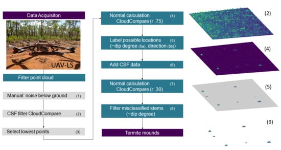
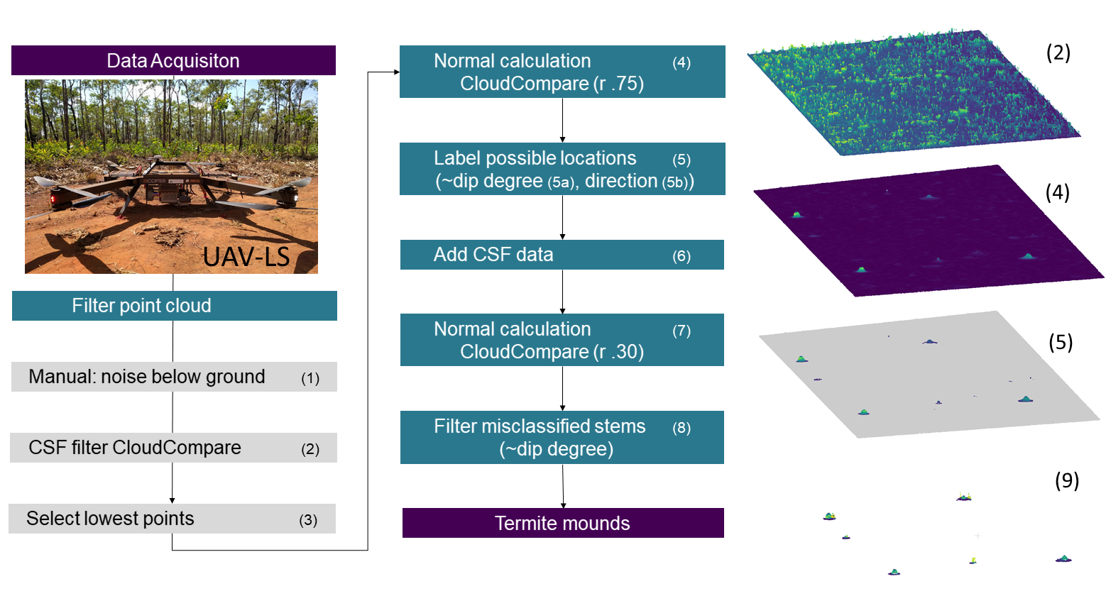
In the first part of the detection algorithm, we created our own ground filtering algorithm, since established algorithms (e.g., the ground filtering algorithm of LAStools, called “LASground”) did not retain the top part of termite mounds. These algorithms also form the basis for digital terrain models (DTMs) and digital surface models (DSMs), which is why we did not use these techniques. The ground filtering that we proposed is rather “conservative” in a way that only the lowest points are kept in a search window of 30 NN in the XY plane. This is a very simple and fast method, which is preferential for large data sets, since the data are heavily reduced. The points are subsequently selected as potential mounds only when a clear slope is present in the data. Our approach achieved good results, which we also credited to the multiple return capabilities of the VUX LiDAR sensor. One beam can receive multiple return signals and partially penetrate through soft material such as leaves, which enables it to delineate the ground floor and its mounds with very high precision.
Our detection algorithm was tested on the geometric position of the points and depended on several empirically defined parameters. The algorithm was designed for the type of termite mounds that have a conical shape. However, many of these parameters can be optimised for other geometric termite mound shapes, or could be optimized to work on UAV-LS data with a different point density. Those parameters are the amount of nearest neighbours (NN) used to extract ground points, the thresholds used to identify mounds using the normal calculations and those that determine which clusters are classified as mounds as opposed to tree stems. Not all these parameters will need to be changed if a different data set is used, but if needed, they are easily adjustable. We thus advise users to first run the algorithm on a small subset of the data using the predefined parameters, to visually check the subsequent steps, and if needed, to alter the parameters. Once these are defined, the algorithm can detect termite mounds with no manual intervention.
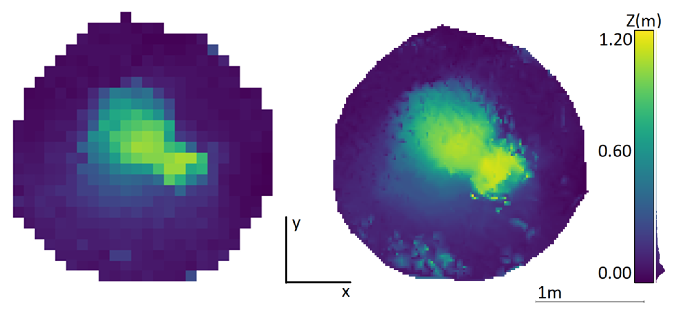
Based on the delineated termite mounds that we derived from the detection algorithm, we were also able to estimate both termite mound height and its volume. Unfortunately, no traditional ground truth data are available, but since TLS is a commonly used method to estimate the volume of (tree) point clouds, with good results, e.g., [34,35], we are confident volume errors are in the same, small, error range. For both the Gaussian approach, in which termite mounds are approximated by fitting a Gaussian distribution to the points, and the grid approach, in which the height is derived from a rasterized point cloud, height estimations were better than volume calculations. For HR data, the grid approach performed only slightly better than the Gaussian approach, but once the resolution lowered, it was outperformed by the Gaussian approach. However, not all mounds were appropriately fitted by the Gaussian approach, and a manual inspection to remove outliers was needed. As with height, the quality of fit for the volume estimations significantly lowered with resolution. We are confident that both volume and height estimations can still be improved, if termite mounds are better delineated in the data. Currently, the estimations are affected by adjacent points, not part of the mound. For termite mounds that grew around stems for example, some of its points were included in the calculations. In both the HR and LR data sets, this resulted in over- and under-estimations, and it influenced the optimized parameters. Alternatively, in future research, termite shape might be approximated using other 3D techniques such as convex hulls.
Even when resolution is low and flight lines are sparse, the acquired resolution with the UAV is, obviously, much higher compared to ALS data. For example, the termite data sets of Kruger National Park on which many studies about termite mound distributions are based [8,13,14] was derived from ALS data with a coverage of one laser shot/m 2 [36]. Macrotermes mounds are large features (up to 10 m wide and 3 m) and therefore more readily detectable. However, while smaller mounds (>50 cm) were still detected, it is uncertain how many were missed, and field validation for small mounds is rare [37]. These ALS point densities are in stark contrast with the UAV-LS data, which still obtained an average return of 680 points/m 2 in the LR data (multiple return scanner). One major limitation of UAVs currently is the limited battery life. the RIEGL RiCOPTER can only effectively map for 15 min with each flight. Especially in remote areas where charging possibilities are limited, this is something to take into consideration. If batteries improve over the coming years, flight time will increase, and data collection will be more time efficient. Another downside is the price tag: commercial state-of-the-art LiDAR scanners remain expensive. Another, less expensive, method to record the 3D surface is structure from motion (SfM). This is a technique in which 2D images are used to create 3D point clouds. Depending on the user’s needs and the site characteristics, SfM can be an adequate alternative for LiDAR, e.g., [22,38,39]. This is however not always the case: in dense forests, for example, SfM cannot sufficiently capture the ground due to high occlusion [22]. Its applicability for termite mound detection in a savanna woodland landscape with an understorey is thus a scope for future research.
Most importantly, our detection algorithm can be used as a first step in the automatic detection of termite mounds over large areas using UAV-LS data. Once an extensive data set is obtained, covering hundreds of hectares, machine learning techniques can be implemented using a similar approach where geometric features are calculated (e.g., eigenvalues, zenith angles, azimuth angles, etc.) for each point considering neighbouring points in different radii. These sets can be used to train an algorithm to detect mounds, since machine learning techniques currently are of sufficient quality to extract complicated geometric figures from LiDAR data (e.g., to extract lianas from dense tropical forest [40]). In addition, sensor fusion of LiDAR and spectral sensors might improve the classification accuracy and is part of further research. Our algorithm can also be adopted for other ecosystem applications, for example the detailed characterisation of microtopography.

5. Conclusions

Our detection algorithm demonstrates the semi-automated detection of termite mounds from UAV-LS data. Eighty-one percent of the termite mounds >50 cm were detected for the HR data set and 72% for the LR data set. For the HR, only exceptionally steep termite mounds or those that were almost completely fused with tree stems were undetected. Our detection algorithm can be a first step in the direction of the extensive detection of termite mounds using UAV-LS, in which not only mere detection is possible, but also 3D information is available, such as height and volume. Based on the need of the user, the selected flight speed and resulting resolution are a trade-off between area and detectability. The UAV-LS (HR) data set performed slightly better in the detection of mounds and could estimate termite mound volume and height more accurately. We demonstrated that the UAV-LS has the potential to provide the required data to do this, with more flexibility and higher point density than ALS. Apart from other LiDAR sensor specific characteristics, the choice between HR and LR flights eventually comes down to area vs. detectability.
UAV-LS termite mound detection algorithm: https://github.com/BarbaraDh/3DTerrain-TermiteMounds.

Author Contributions

Design of study, K.C., B.D. and H.V.; methodology, K.C., B.D., H.B. and H.V.; data collection K.C., B.D., H.B., T.W., S.L. and R.B.; analysis, K.C., B.D. and H.B.; B.D. led the writing of the manuscript with input from all the authors. All authors read and agreed to the published version of the manuscript.

Funding

H.V. and K.C. were funded by BELSPO (Belgian Science Policy Office) in the frame of the STEREO III programme—project 3D-FOREST (SR/02/355). H.V., K.C. and B.D. were funded by BELSPO (Belgian Science Policy Office) in the frame of the STEREO III programme—project 3D-TERRAIN (SR/02/394).

Institutional Review Board Statement

Not applicable.

Informed Consent Statement

Not applicable.

Data Availability Statement

Data available on request.

Acknowledgments

We acknowledge the Ecosystem Processes facility in Australia’s Terrestrial Ecosystem Research Network (TERN) and NT Parks and Wildlife. We thank Linda Luck and Jodie Hayward for assistance with the fieldwork.

Conflicts of Interest

The authors declare no conflict of interest. The funders had no role in the design of the study; in the collection, analyses, or interpretation of data; in the writing of the manuscript; nor in the decision to publish the results.

Abbreviations

The following abbreviations are used in this manuscript:
LiDARLight detection and ranging
UAVUnmanned aerial vehicle
LSLaser scanning
HRHigh resolution
LRLow resolution
TLSTerrestrial laser scanning
ALSAerial laser scanning
SfMStructure from Motion
NNNearest neighbours
DTMDigital terrain model
DSMDigital surface model
CCCConcordance correlation coefficient

Appendix A

Figure A1. UAV-LS (LR) point cloud. The colour code represents the height above the terrain. The lines represent the recorded flight lines of F1 (UAV-LS (HR)) and F2 (UAV-LS (LR)). Only sections of the flight lines that were used in the registered point clouds are visualized.
Remotesensing 13 00476 g0a1

References

  1. Scholes, R.; Archer, S. Tree-grass interactions in savannas. Annu. Rev. Ecol. Syst. 1997, 28, 517–544. [Google Scholar] [CrossRef]
  2. Bonachela, J.A.; Pringle, R.M.; Sheffer, E.; Coverdale, T.C.; Guyton, J.A.; Caylor, K.K.; Levin, S.A.; Tarnita, C.E. Termite mounds can increase the robustness of dryland ecosystems to climatic change. Science 2015, 347, 651–655. [Google Scholar] [CrossRef] [Green Version]
  3. Mando, A.; Brussaard, L.; Stroosnijder, L. Termite-and mulch-mediated rehabilitation of vegetation on crusted soil in west Africa. Restor. Ecol. 1999, 7, 33–41. [Google Scholar] [CrossRef]
  4. Davies, A.B.; Brodrick, P.G.; Parr, C.L.; Asner, G.P. Resistance of mound-building termites to anthropogenic land-use change. Environ. Res. Lett. 2020, 15, 094038. [Google Scholar] [CrossRef]
  5. Holt, J.A.; Lepage, M. Termites and soil properties. In Termites: Evolution, Sociality, Symbioses, Ecology; Springer: Berlin/Heidelberg, Germany, 2000; pp. 389–407. [Google Scholar]
  6. Sileshi, G.W.; Arshad, M.; Konaté, S.; Nkunika, P.O. Termite-induced heterogeneity in African savanna vegetation: Mechanisms and patterns. J. Veg. Sci. 2010, 21, 923–937. [Google Scholar] [CrossRef]
  7. Ahmed, J.B.; Pradhan, B. Termite mounds as bio-indicators of groundwater: Prospects and constraints. Pertanika J. Sci. Technol. 2018, 26, 479–498. [Google Scholar]
  8. Davies, A.B.; Baldeck, C.A.; Asner, G.P. Termite mounds alter the spatial distribution of African savanna tree species. J. Biogeogr. 2016, 43, 301–313. [Google Scholar] [CrossRef]
  9. Levick, S.R.; Asner, G.P.; Kennedy-Bowdoin, T.; Knapp, D.E. The spatial extent of termite influences on herbivore browsing in an African savanna. Biol. Conserv. 2010, 143, 2462–2467. [Google Scholar] [CrossRef]
  10. Sanderson, M. Biomass of termites and their emissions of methane and carbon dioxide: A global database. Glob. Biogeochem. Cycles 1996, 10, 543–557. [Google Scholar]
  11. Kirschke, S.; Bousquet, P.; Ciais, P.; Saunois, M.; Canadell, J.G.; Dlugokencky, E.J.; Bergamaschi, P.; Bergmann, D.; Blake, D.R.; Bruhwiler, L.; et al. Three decades of global methane sources and sinks. Nat. Geosci. 2013, 6, 813–823. [Google Scholar] [CrossRef]
  12. Nauer, P.A.; Chiri, E.; Souza, D.d.; Hutley, L.B.; Arndt, S.K. Rapid image-based field methods improve the quantification of termite mound structures and greenhouse-gas fluxes. Biogeosciences 2018, 15, 3731–3742. [Google Scholar] [CrossRef] [Green Version]
  13. Levick, S.R.; Asner, G.P.; Chadwick, O.A.; Khomo, L.M.; Rogers, K.H.; Hartshorn, A.S.; Kennedy-Bowdoin, T.; Knapp, D.E. Regional insight into savanna hydrogeomorphology from termite mounds. Nat. Commun. 2010, 1, 65. [Google Scholar] [CrossRef] [PubMed]
  14. Davies, A.B.; Levick, S.R.; Asner, G.P.; Robertson, M.P.; van Rensburg, B.J.; Parr, C.L. Spatial variability and abiotic determinants of termite mounds throughout a savanna catchment. Ecography 2014, 37, 852–862. [Google Scholar] [CrossRef]
  15. Davies, A.B.; Parr, C.L.; Janse Van Rensburg, B. Termites and fire: Current understanding and future research directions for improved savanna conservation. Austral Ecol. 2010, 4, 482–486. [Google Scholar]
  16. Jones, C.G.; Lawton, J.H.; Shachak, M. Organisms as ecosystem engineers. In Ecosystem Management; Springer: Berlin/Heidelberg, Germany, 1994; pp. 130–147. [Google Scholar]
  17. Grohmann, C.; Oldeland, J.; Stoyan, D.; Linsenmair, K. Multi-scale pattern analysis of a mound-building termite species. Insectes Sociaux 2010, 57, 477–486. [Google Scholar] [CrossRef]
  18. Mujinya, B.B.; Adam, M.; Mees, F.; Bogaert, J.; Vranken, I.; Erens, H.; Baert, G.; Ngongo, M.; Van Ranst, E. Spatial patterns and morphology of termite (Macrotermes falciger) mounds in the Upper Katanga, DR Congo. Catena 2014, 114, 97–106. [Google Scholar] [CrossRef]
  19. Wyngaard, J.; Barbieri, L.; Thomer, A.; Adams, J.; Sullivan, D.; Crosby, C.; Parr, C.; Klump, J.; Raj Shrestha, S.; Bell, T. Emergent challenges for science sUAS data management: Fairness through community engagement and best practices development. Remote Sens. 2019, 11, 1797. [Google Scholar] [CrossRef] [Green Version]
  20. Resop, J.P.; Lehmann, L.; Hession, W.C. Drone Laser Scanning for Modeling Riverscape Topography and Vegetation: Comparison with Traditional Aerial Lidar. Drones 2019, 3, 35. [Google Scholar] [CrossRef] [Green Version]
  21. Lin, Y.C.; Cheng, Y.T.; Zhou, T.; Ravi, R.; Hasheminasab, S.M.; Flatt, J.E.; Troy, C.; Habib, A. Evaluation of UAV LiDAR for mapping coastal environments. Remote Sens. 2019, 11, 2893. [Google Scholar]
  22. Wallace, L.; Lucieer, A.; Malenovskỳ, Z.; Turner, D.; Vopěnka, P. Assessment of forest structure using two UAV techniques: A comparison of airborne laser scanning and structure from motion (SfM) point clouds. Forests 2016, 7, 62. [Google Scholar] [CrossRef] [Green Version]
  23. Brede, B.; Calders, K.; Lau, A.; Raumonen, P.; Bartholomeus, H.M.; Herold, M.; Kooistra, L. Non-destructive tree volume estimation through quantitative structure modelling: Comparing UAV laser scanning with terrestrial LIDAR. Remote Sens. Environ. 2019, 233, 111355. [Google Scholar] [CrossRef]
  24. Brede, B.; Lau, A.; Bartholomeus, H.M.; Kooistra, L. Comparing RIEGL RiCOPTER UAV LiDAR derived canopy height and DBH with terrestrial LiDAR. Sensors 2017, 17, 2371. [Google Scholar] [CrossRef] [PubMed]
  25. TERN. Litchfield Savanna SuperSite. Available online: http://www.tern-supersites.net.au/supersites/lfld (accessed on 23 November 2020).
  26. Calders, K.; Adams, J.; Armston, J.; Bartholomeus, H.; Bauwens, S.; Bentley, L.P.; Chave, J.; Danson, F.M.; Demol, M.; Disney, M.; et al. Terrestrial laser scanning in forest ecology: Expanding the horizon. Remote Sens. Environ. 2020, 251, 112102. [Google Scholar] [CrossRef]
  27. Luck, L.; Hutley, L.B.; Calders, K.; Levick, S.R. Exploring the Variability of Tropical Savanna Tree Structural Allometry with Terrestrial Laser Scanning. Remote Sens. 2020, 12, 3893. [Google Scholar] [CrossRef]
  28. CloudCompare v2.11.3. [GPL Software] CloudCompare. 2020. Available online: http://www.cloudcompare.org (accessed on 23 November 2020).
  29. Cook, R.L. Stochastic sampling in computer graphics. ACM Trans. Graph. (TOG) 1986, 5, 51–72. [Google Scholar]
  30. Dippé, M.A.; Wold, E.H. Antialiasing through stochastic sampling. In Proceedings of the 12th Annual Conference on Computer Graphics and Interactive Techniques, San Francisco, CA, USA, 22–26 July 1985; pp. 69–78. [Google Scholar]
  31. Contributors, P. PDAL Point Data Abstraction Library. 2018. Available online: pdal.io/references.html (accessed on 28 January 2021). [CrossRef]
  32. Zhang, W.; Qi, J.; Wan, P.; Wang, H.; Xie, D.; Wang, X.; Yan, G. An easy-to-use airborne LiDAR data filtering method based on cloth simulation. Remote Sens. 2016, 8, 501. [Google Scholar] [CrossRef]
  33. Burt, A.; Disney, M.; Calders, K. Extracting individual trees from lidar point clouds using treeseg. Methods Ecol. Evol. 2019, 10, 438–445. [Google Scholar]
  34. Calders, K.; Newnham, G.; Burt, A.; Murphy, S.; Raumonen, P.; Herold, M.; Culvenor, D.; Avitabile, V.; Disney, M.; Armston, J.; et al. Nondestructive estimates of above-ground biomass using terrestrial laser scanning. Methods Ecol. Evol. 2015, 6, 198–208. [Google Scholar] [CrossRef]
  35. Fabbri, S.; Giambastiani, B.M.; Sistilli, F.; Scarelli, F.; Gabbianelli, G. Geomorphological analysis and classification of foredune ridges based on Terrestrial Laser Scanning (TLS) technology. Geomorphology 2017, 295, 436–451. [Google Scholar] [CrossRef]
  36. Asner, G.P.; Knapp, D.E.; Kennedy-Bowdoin, T.; Jones, M.O.; Martin, R.E.; Boardman, J.W.; Field, C.B. Carnegie airborne observatory: In-flight fusion of hyperspectral imaging and waveform light detection and ranging for three-dimensional studies of ecosystems. J. Appl. Remote Sens. 2007, 1, 013536. [Google Scholar] [CrossRef]
  37. Lind, B.M.; Hanan, N.P.; Gigliotti, L.C.; Allen, R.L.; McHenry, A.; Gardiner, A. Termite diversity along a catena in southern Kruger National Park, South Africa. Afr. J. Ecol. 2019, 57, 160–165. [Google Scholar] [CrossRef] [Green Version]
  38. Fonstad, M.A.; Dietrich, J.T.; Courville, B.C.; Jensen, J.L.; Carbonneau, P.E. Topographic structure from motion: A new development in photogrammetric measurement. Earth Surf. Process. Landf. 2013, 38, 421–430. [Google Scholar] [CrossRef] [Green Version]
  39. Nouwakpo, S.K.; Weltz, M.A.; McGwire, K. Assessing the performance of structure-from-motion photogrammetry and terrestrial LiDAR for reconstructing soil surface microtopography of naturally vegetated plots. Earth Surf. Process. Landf. 2016, 41, 308–322. [Google Scholar] [CrossRef]
  40. Bao, Y.; Moorthy, S.; Verbeeck, H. Towards extraction of lianas from terrestrial lidar scans of tropical forests. In Proceedings of the IGARSS 2018–2018 IEEE International Geoscience and Remote Sensing Symposium, Valencia, Spain, 22–27 July 2018; pp. 7544–7547. [Google Scholar]
Figure 1. UAV-LS (low resolution) point cloud, indicating the boundaries of all data types. The colour code represents the height above terrain. The maximum tree height is approximatively 25 m, and the open canopy allows a substantial understorey.
Remotesensing 13 00476 g001
Figure 2. RIEGL RiCOPTER with VUX-1UAV.
Remotesensing 13 00476 g002
Figure 3. Overview of the main steps to extract termite mounds from UAV-LS data. CSF, cloth simulation filter.
Remotesensing 13 00476 g003
Figure 4. A termite mound in the UAV-LS (HR) point cloud. Points are first filtered based on dip degree; if this value falls outside the interval [7°, 86°], points are rejected. Then, data are clustered, and only point clusters that have more than 50 points are considered. The white points are the rejected points.
Remotesensing 13 00476 g004
Figure 5. The dip direction represents the direction of the slope. Since the termite mounds have a conical shape, this value should alter from 0 to 360 degrees around the centre of the mound. If the optimized centre is located > 0.75 m from the mean position of the cluster or if the RMSE of optimization > 1, the cluster is rejected. The grey lines are contour lines (height). In this figure, the approved cluster is a termite mound, while the rejected cluster is a fallen tree trunk. Taken from the UAV-LS (HR) data set.
Remotesensing 13 00476 g005
Figure 6. To estimate termite mound height, a large grid size was used to avoid the influence from outliers (left). To calculate volume, a smaller grid size was used. Since the volume was calculated as the sum of many small cuboids, possible outliers had less influence (right).
Remotesensing 13 00476 g006
Figure 7. Rasterized point cloud for volume calculation (UAV-LS (HR)). The cuboids that are used to estimate the volume are confined by the top line and the termite mound. The bottom line represents the average height of the lowest 20 points. The value of n was optimized to prevent over- or under-estimations of termite mound volume.
Remotesensing 13 00476 g007
Figure 8. Locations of the mounds derived from the 1 ha benchmark data set. + (plus) means the mound is detected; − (minus) means it is not detected by the UAV-LS detection algorithm. The grey mounds are small mounds <50 cm that could only be detected in the benchmark data set.
Remotesensing 13 00476 g008
Figure 9. A visualisation of all detected termite mounds in the 1 ha benchmark data set that could be manually identified, ordered according to their height. The Y-axis represents the height above terrain, while the X-axis represents the front view of the mounds. The axes are equally scaled. Our focus is termite mounds >0.5 m height.
Remotesensing 13 00476 g009
Figure 10. One termite mound, three different methods of acquisition. The point clouds consist of respectively 21,907, 5553 and 1107 points. All methods are able to adequately record termite mound shape.
Remotesensing 13 00476 g010
Figure 11. Scatter plot with linear regressions of the height estimations, validated using the benchmark data set. The top three plots show results from the Gaussian approach and the bottom three from the grid approach.
Remotesensing 13 00476 g011
Figure 12. Linear regressions of termite mound volume (raster: 2 cm) for the benchmark data set and the UAV-LS data sets.
Remotesensing 13 00476 g012
Table 1. Specifications of the three data sets.
TypeTLSUAV-LS F1 (HR)UAV-LS F2 (LR)
Scanner/cameraLeica BLK360VUX-SYSVUX-SYS
Wavelength (nm)83015501550
Beam divergence (mrad)0.40.50.5
Scanning pattern20 × 20 mrandomoutline + 11 crosses
Point density (pts/m 2 )∼2200∼1800∼680
Flying speed (m/s)NA35
Area (ha)1∼9.8∼34
Table 2. Overview of the user-adjustable parameters of the termite mound detection algorithm.
Step (Figure 3)Parameters
1: Manually filter noise below ground-
2: Cloth Simulation Filterscene: steep slope, cloth resolution: 1.0, max. iterations: 500, classification threshold: 1
3: Select low pointsk: 30 NN
4: Normal calculationradius: 0.75 m
5a: Label locations (filter on dip degree)dip degree: 7 –87 ; if <50 NN within 1 m, point is discarded
5b: Label locations (optimize centre)distance <0.75 m; RMSE < 1
7: Normal calculationradius: 0.30 m
8: Filter stemsall clusters of which >77% of points (above 15 cm ground surface) having a dip degree >77 are discarded
Table 3. Detected termite mounds per hectare (>50 cm) using our detection algorithm for the UAV-LS data sets. * mounds detected in the benchmarking area.
Mound DensityMounds DetectedAreaMounds Detected *
TLS11 mounds/ha11 mounds1 ha11 mounds
UAV-LS (HR)8 mounds/ha79 mounds9.8 ha9 mounds
UAV-LS (LR)6.9 mounds/ha322 mounds34 ha8 mounds
Table 4. Linear regressions and CCC of the height estimations using the Gaussian approach. For the top 2 rows, the benchmark data set is used as validation.
R 2 p ValueCCCScale ShiftLocation Shift (m)Bias Correction
UAV-LS (HR)0.866.5 × 10 10 0.871.24 0.30 0.93
UAV-LS (LR)0.848.2 × 10 8 0.831.43 0.26 0.91
UAV-LS (HR vs. LR)0.601.637 × 10 14 0.771.04 0.01 1.00
Table 5. Linear regressions and CCC of the height estimations using the grid approach. For the top 2 rows, the benchmark data set is used as validation.
R 2 p ValueCCCScale ShiftLocation Shift (m)Bias Correction
UAV-LS (HR)0.868 × 10 9 0.931.020.071.00
UAV-LS (LR)0.601.50 × 10 4 0.761.08 0.18 0.98
UAV-LS (HR vs. LR)0.593.836 × 10 14 0.701.10 0.41 0.92
Table 6. Linear regressions and CCC of the volume estimations. For the top 2 rows, the benchmark data set is used as validation.
R 2 p ValueCCCScale ShiftLocation Shift (m)Bias Correction
UAV-LS (HR)0.785.42 × 10 7 0.880.950.021.00
UAV-LS (LR)0.664.56 × 10 5 0.781.18 0.25 0.96
UAV-LS (HR vs. LR)0.638.88 × 10 16 0.531.500.920.66
Publisher’s Note: MDPI stays neutral with regard to jurisdictional claims in published maps and institutional affiliations.

