Abstract
The United Nations’ expanded program for Reducing Emissions from Deforestation and Forest Degradation (REDD+) aims to mobilize capital from developed countries in order to reduce emissions from these sources while enhancing the removal of greenhouse gases (GHGs) by forests. To achieve this goal, an agreement between the Parties on reference levels (RLs) is critical. RLs have profound implications for the effectiveness of the program, its cost efficiency, and the distribution of REDD+ financing among countries. In this paper, we introduce a methodological framework for setting RLs for REDD+ applications in tropical forests in Xishuangbanna, China, by coupling the Good Practice Guidance on Land Use, Land Use Change, and Forestry of the Intergovernmental Panel on Climate Change and land use scenario modeling. We used two methods to verify the accuracy for the reliability of land classification. Firstly the accuracy reached 84.43%, 85.35%, and 82.68% in 1990, 2000, and 2010, respectively, based on high spatial resolution image by building a hybrid matrix. Then especially, the 2010 Globeland30 data was used as the standard to verify the forest land accuracy and the extraction accuracy reached 86.92% and 83.66% for area and location, respectively. Based on the historical land use maps, we identified that rubber plantations are the main contributor to forest loss in the region. Furthermore, in the business-as-usual scenario for the RLs, Xishuangbanna will lose 158,535 ha (158,535 × 104 m2) of forest area in next 20 years, resulting in approximately 0.23 million t (0.23 × 10⁹ kg) CO2e emissions per year. Our framework can potentially increase the effectiveness of the REDD+ program in Xishuangbanna by accounting for a wider range of forest-controlled GHGs.
1. Introduction
Forests account for almost half of the global terrestrial carbon pool, and the vegetation within them alone (excluding soils) holds approximately 75% of all living carbon. The total carbon content in forest ecosystems is estimated to be 638 Gt [1,2,3,4,5]. Tropical forests play a particularly important role in the global carbon budget because they contain as much carbon in their vegetation and soils as all the temperate-zone and boreal forests combined [6,7,8,9,10,11,12]. Per unit area, tropical forests store, on average, approximately 50% more carbon than their nontropical counterparts. Scientists agree that to achieve the goals of the United Nation’s Framework Convention on Climate Change (UNFCCC), namely avoiding irreversible damage to the climate system, global warming must not exceed 2 °C [13,14,15,16]. However, concentrations of CO2 in the atmosphere are already so high that global emissions will likely peak before they start to decline. Thus, in order to remain under the above-mentioned threshold, emissions from all major sources (i.e., from developed countries, major developing country emitters, and deforestation) must begin to decline within the next decade [17,18,19].
The Conference of the Parties (COP) agreed that Reducing Emissions from Deforestation and Forest Degradation (REDD+) with the enhancement of the removal of greenhouse gas (GHG) emissions by forests in developing countries could support the goals of the framework through the positive incentives provided by the UNFCCC. The general consensus at Doha in 2012 following last year’s COP17 was that the results of financing, safeguards, measurements, and reporting and verification for REDD+ were mixed. In addition, significant progress has been widely recognized as having been made only within the technical arena relating to reference levels (RLs). The 19th Conference of the Parties to the UNFCCC (COP19) and the 9th Conference of the Parties to the Kyoto Protocol (CMP9) were jointly held on the topic of REDD+ funding in Warsaw, Poland, and in-depth discussions on the action points were conducted.
GHG-based compensation for REDD+ requires an agreement on emission RLs. Key elements for setting these RLs include the ability to measure changes throughout all forested areas, the use of consistent methodologies at repeated intervals to obtain accurate results, and the verification of results with ground-based or very high-resolution observations [20,21,22,23,24]. RLs have profound implications for the effectiveness of climate-related policies, cost efficiency, and distribution of REDD+ financing, and they involve a number of tradeoffs [25,26,27,28,29,30]. In this paper, referring to the business-as-usual scenario, we introduce a methodological framework for setting RLs for REDD+ applications in tropical forests in Xishuangbanna, China, by coupling the Good Practice Guidance (GPG) on Land Use, Land Use Change, and Forestry published by the Intergovernmental Panel on Climate Change (IPCC) and land use scenario modeling. This study contributes to the literature by highlighting key challenges for setting RLs as part of the REDD+ program.
2. Data and Methodology
2.1. Research Area
Not only is the forest in the Xishuangbanna region (Figure 1) the world’s largest preserved area located in the northernmost part of the Earth, but it is home to the majority of tropical forest ecosystems in China as well. The geology, climate, and soil of Xishuangbanna are suitable for the growth and reproduction of various organisms. Moreover, 4500 species of higher plants have been recorded in Xishuangbanna, accounting for about one-seventh of the total number of higher plants in China. The native vegetation types include those found in tropical rain forests, montane rain forests, tropical monsoon forests, subtropical evergreen broad-leaved forests, deciduous broad-leaved forests, warm coniferous forests, and bamboo forests as well as shrubs and grasses [31,32,33,34]. In recent years, due to the increase in the population, intensification of anthropogenic activities, the enabling climate, and suitable terrain conditions in the area, the cultivation of rubber and other tropical and economically important crops has risen rapidly. Thus, the changes to the forest have been very dramatic.
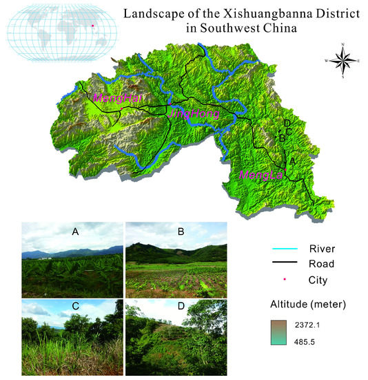
Figure 1.
Landscape of the Xishuangbanna, China.
2.2. IPCC’s Good Practice Guidance
The IPCC’s existing GPG for Land Use, Land Use Change, and Forestry provides the recommended approach to account for fluctuations in carbon stocks resulting from changes in the use and management of forests. This framework has been accepted by all Parties in the Bali Action Plan of COP13 [35,36,37]. The IPCC’s GPG framework refers to two basic inputs for forest carbon accounting, namely activity data and emission factors. Activity data in the REDD+ context refer to the areal extent of emissions. For example, in the context of deforestation, activity data refer to the area of deforestation, presented in hectares (104 m2) over a known time period. Emission factors refer to the emission or removal of GHGs per unit activity. The emission or removal of GHGs resulting from land use conversion ultimately alters ecosystem carbon stocks.
2.2.1. Emissions Factors
To estimate emissions factors, the required number of sample plots was determined to the necessary accuracy using the size of the forest area and other available resources. Provisional surveys and/or existing data can be utilized to establish sample sizes, and tools also exist to calculate sample sizes based on fixed precision levels or given fixed inventory costs [38,39,40,41]. In the event carbon stocks and flows are to be monitored over the long term, permanent sites should be considered in order to reduce between-site variability and to capture actual trends as opposed to short-term fluctuations [42].
In the study, the aboveground biomass density map was sourced from Global Forest Watch (http://www.globalforestwatch.org/). This map is a global aboveground biomass density map produced in 2000 according to the method devised by Baccini [43]. Based on the improved methodology, the resolution can be increased to as much as 30 m. The aboveground biomass density map of Xishuangbanna region was extracted using the mask extraction method.
More recently, Maurizio Santoro [44] have proposed an integration methodology for estimation of aboveground biomass density for around the year 2010 by combining SAR, LiDAR, and optical observations together with other datasets such as auxiliary datasets from forest inventories, additional remote sensing observations, climate variables, and ecosystems classifications. We compared with the latest biomass map developed by Santoro against Global Forest Watch product.
2.2.2. Activity Data
Estimation of activities associated with national-level deforestation monitoring is practically possible only via remote sensing [45,46,47,48,49]. Since the early 1990s, changes in forest area have been monitored from space with confidence. Some countries have had well-established operational systems for over a decade.
Taking into account the availability of the data and their matching, this study used the Enhanced Thematic Mapper Plus/Thematic Mapper (ETM+/TM) remote sensing images related to Path number 130 and Row number 044, Path number 131 and Row number 045, Path number 130 and Row number 045, Path number 129 and Row number 045 in the study area in 1990, 2000, and 2010 to interpret land use changes(Table 1). The TM/ETM+ remote sensing images and normalized difference vegetation index (NDVI) data were sourced from the US Geological Survey (USGS, http://earthexplorer.usgs.gov/). We mosaiced the TM/ETM+ remote sensing images of the same year, used ENVI to perform geometric correction and radiometric correction, converted all the map data projections to WGS84/UTM Zone47N (EPSG: 32647), used the Xishuangbanna administrative vector map for mask extraction, and performed cropping to obtain the images of Xishuangbanna.

Table 1.
Landsat imagery used in this study.
The vegetation in the study area changes obviously with the seasons, and the NDVI values at different times, thus, have a greater influence on the research results. Thus, this study synthesized the maximum value of the NDVI data in multiple phases of the same year and also eliminated the influence of cloud cover on the research results.
According to the characteristics of land use cover in the study area (Table 2), we divided the land use cover into eight types: forestland, shrubland, grassland, cultivated land, rubber forest, tea gardens, construction land, and water. The training samples were determined using QuickBird images in Google Earth. The terrain of the study area is relatively complex, and many “homogeneous spectrum” phenomena occur in the interpretation of remote sensing images. To avoid this phenomenon, it is necessary to select as many training samples as possible. Different band combinations of Landsat7 ETM images have different characteristics. The selection of the training samples was carried out according to these characteristics. The ETM541 band combination is helpful for distinguishing different vegetation types when supplemented by NDVI data. The training samples of natural forests, shrubs, rubber plantations, and tea gardens were selected. The ETM453 band combination was used to select the cultivated land and water, while the construction land was extracted through the ETM743 band combination, and the remainder was categorized as other land. Supervised classification was performed using the selected training samples to obtain the preliminary classification results, and the accuracy test was conducted. If the results did not agree, the training samples were reselected, and the supervised classification and accuracy tests were reperformed until they were ideal. Finally, the classification results were recoded, clustered, and eliminated, and the broken patches were merged into the adjacent largest classification to unify the smallest unit.

Table 2.
Land use classification followed for this study.
The Land Use Dynamic Index considers the transfer of land use types during the study period, and reflects the intensity of regional land use changes during this time. It is essential to find hot spots of land use changes at different spatial scales. It is one of the important parameters to analyze the dynamic changes in land use space [50]. Equation (1) was used to calculate the index.
Ki is the land use dynamic degree for land use type i in a certain period of time, and are the number of certain land use types at the start of the period t1 and its end t2, respectively, and t2 − t1 is the research duration.
is the comprehensive land use dynamic degree in the study area corresponding to time period. is the area of land use type converted converted to other land use types in the study period; is the area of type land use type at the beginning of the study; is the time period of land use change.
2.3. Land Use Scenario Modeling for Reference Levels
Land use simulation is based on years of known land use changes. It predicts future land use changes. Most land use models used to simulate the process of land use change typically need to solve two problems: the quantity problem and the distribution problem. The quantity problem refers to how much of the land area has changed, while the distribution problem involves pinpointing where those land changes occurred. This study applied the Land Change Modeler (LCM) [51,52,53], which uses the Markov chain model to predict the number of future land use changes, and then calculates the distribution location of these changes according to the Multilayer Perceptron (MLP) model.
Markov chain is a kind of “no after-effect” random stored procedure, as it assumes that the state of the current variable is only related to its previous state, not to its states at other moments. Therefore, it has good operability and is used in the simulation of various land use changes. In Equation (3) of Markov chain, for any positive integer n and possible states , ..., of the random variables,
As the land use change conforms to the basic characteristics of the Markov process, it can be regarded as a Markov process. Therefore, the Markov chain analysis can describe the land use change process and predict the future land use change trend. It is an important transformation tool in land use change modeling. However, the following prerequisites must be fulfilled [54,55,56]: (1) In a certain area, different types of land use should be transformable into each other, (2) the conversion between different types of land use can include many events, which are difficult to describe with a specific formula, and (3) within the time limit of the study, the conversion status of the land use structure is relatively stable, which meets the requirements of the Markov chain. Moreover, the area ratio of the mutual conversion between the types of land uses equals the state transition probability.
MLP is a very widely used neural network in remote-sensing image processing, especially remote sensing image classification. MLP was used in the model primarily to calculate the land use change potential, that is, the future conversion probability between each land use type. The process involved analyzing future land use by establishing a land use driving force model and the quantitative relationship between each land use type to assess the probability of change. Based on the calculated potential distribution of soil use changes, the location of possible future land use changes can be determined. The back propagation algorithm used in MLP consists of two parts, namely the forward propagation of information and the backward propagation of errors. In the forward propagation process, the input information is calculated from the input layer through the hidden layer to the output layer, and each layer for the state of a neuron only affects the state of the next layer of neurons [57,58]. If the expected output is not obtained in the output layer, the error change value of the output layer is calculated, and then turned to reverse propagation, and the error signal is returned back along the original connection path through the network to modify the weights of neurons in each layer until the desired target is reached. During the forward propagation process, the state of the activated neuron is updated layer-by-layer from the input layer to the output layer, as shown in Equation (4):
xj represents the total input received by neuron j, wji represents the weight between neurons j and i, αi denotes neuron i once xj is calculated. The most commonly used mapping function is the S (sigmoid) function, as shown in Equation (5).
It is crucial to check the accuracy and effect of the model to determine whether the model needs to be adjusted. The Receiver Operating Characteristic (ROC) curve test evaluates the model by comparing the predicted land change probability distribution map with the actual changed 0–1 map (the changed land value is 1, and the unchanged land value is 0) [59,60,61]. This step converts the simulated and reference images into a 2 × 2 table, with each table corresponding to a different threshold. The number of pixels within the thresholds of A, B, C, and D create the statistical figure for each ROC curve threshold. The following data are produced; x and y form the point (x, y), where x is the ratio of classifications labeled as true−, namely D/(B + D), and y is the proportion of true+ classifications, that is, A/(A + C). In order to be expressed as a positive value on the x axis, the opposite part of true− is generally represented by B/(B + D). Thus, the ROC curve test provides the Area Under the ROC Curve (AUC), which is obtained using the following formula:
where xi refers to x for each threshold i, that is, B/(B + D), and y is calculated using D/(B + D).
3. Results and Discussion
3.1. Analysis of Historical Land Use
The land use maps in 1990, 2000, and 2010 and the accuracies are shown in Figure 2 and Appendix A. Firstly we randomly generated 2866, 2549, and 2481 sample points in 1990, 2000, and 2010 through hierarchical random sampling method. There were 1520 sample points, 1227 sample points, and 1008 sample points in forest area in 1990, 2000, and 2010, respectively. Then we evaluated the accuracy of classification for sample points based on Google earth.
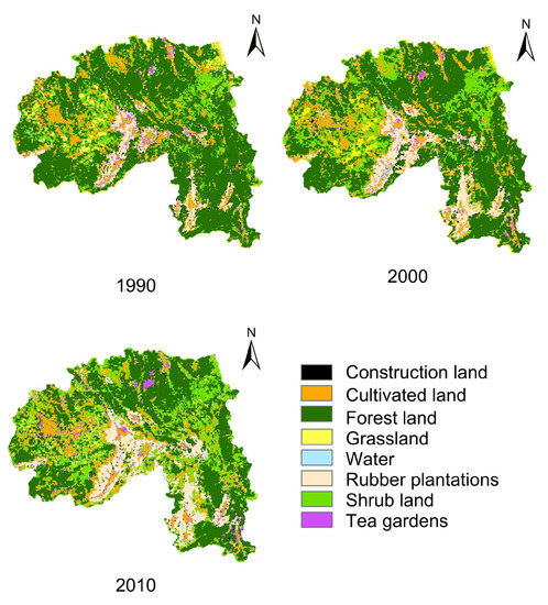
Figure 2.
Land use maps and the accuracies in 1990, 2000, and 2010.
GlobeLand30, which was developed by the National Geomatics Center of China, is an open-access 30m resolution global land cover data product with an overall classification accuracy of over 80% [62,63]. We compared the area and spatial location of the forest land in 2010 extracted by Globeland30 with those in this study (Figure 3). Firstly, about 600 sample points are randomly generated within Xishuangbanna administrative region. Then these sample points are overlapped with Globeland30 and land use map respectively. Finally we evaluate the accuracy of land use map based on the consistency of forest land and nonforest land in Globeland30.
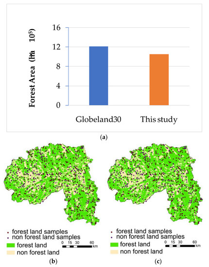
Figure 3.
(a) Forest area in 2010 from Globeland30 and this study; (b)spatial distribution of the validation samples in Globeland30; (c) spatial distribution of the validation samples in this study.
In terms of the forest land area, the forest land area extracted from Globeland30 was 1.21× 10⁶ ha, and that from this study is 1.05×10⁶ ha, with the accuracy 86.92%. In terms of spatial location of the forest land, among 600 randomly generated sample points, 376 were the forest land and 230 were nonforest land in Globeland30; in comparison, 331 sample points were the forest land and 275 sample points were nonforest land in this study. The overall accuracy is 83.66%, and the kappa coefficient is 0.657.
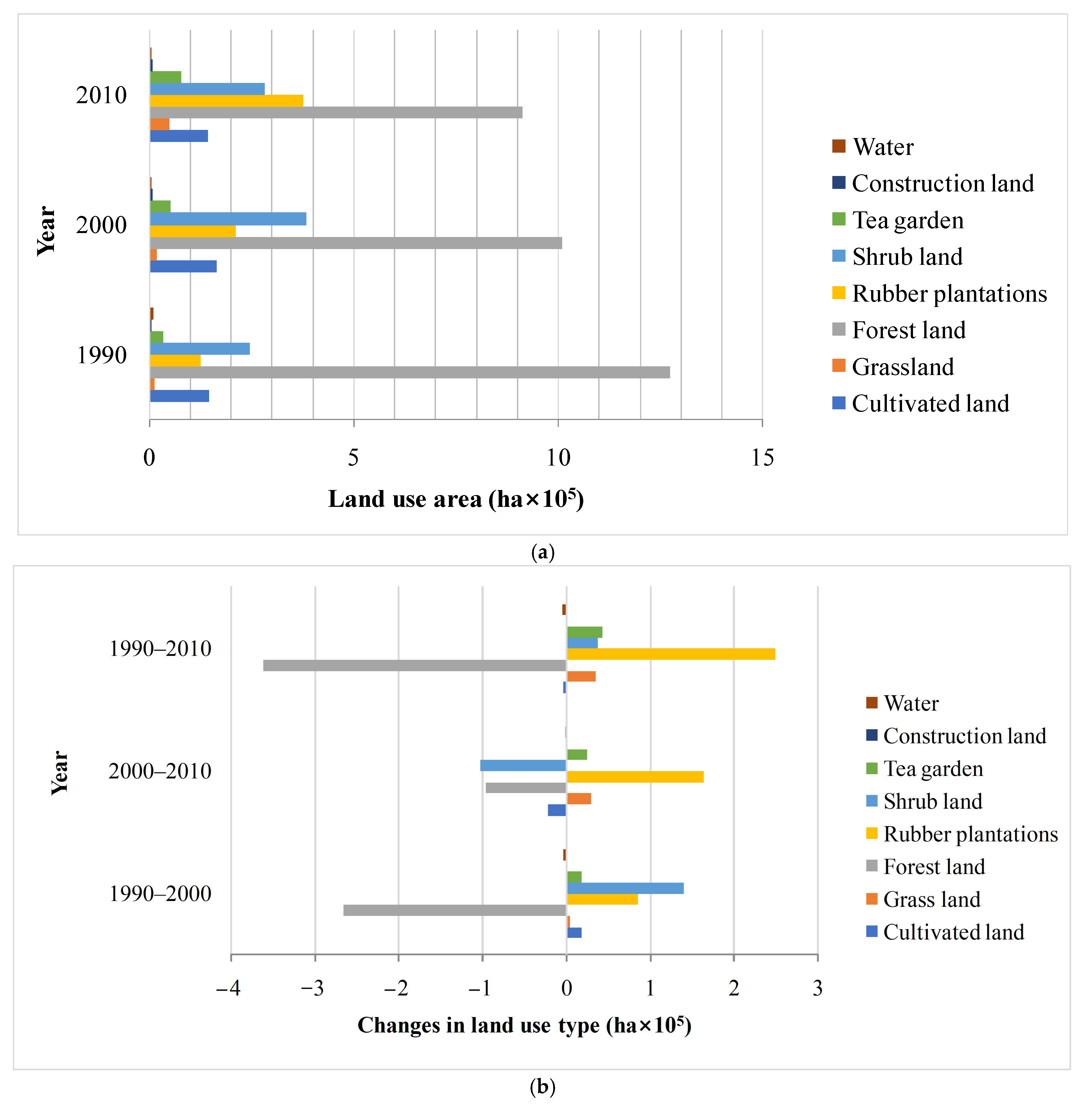
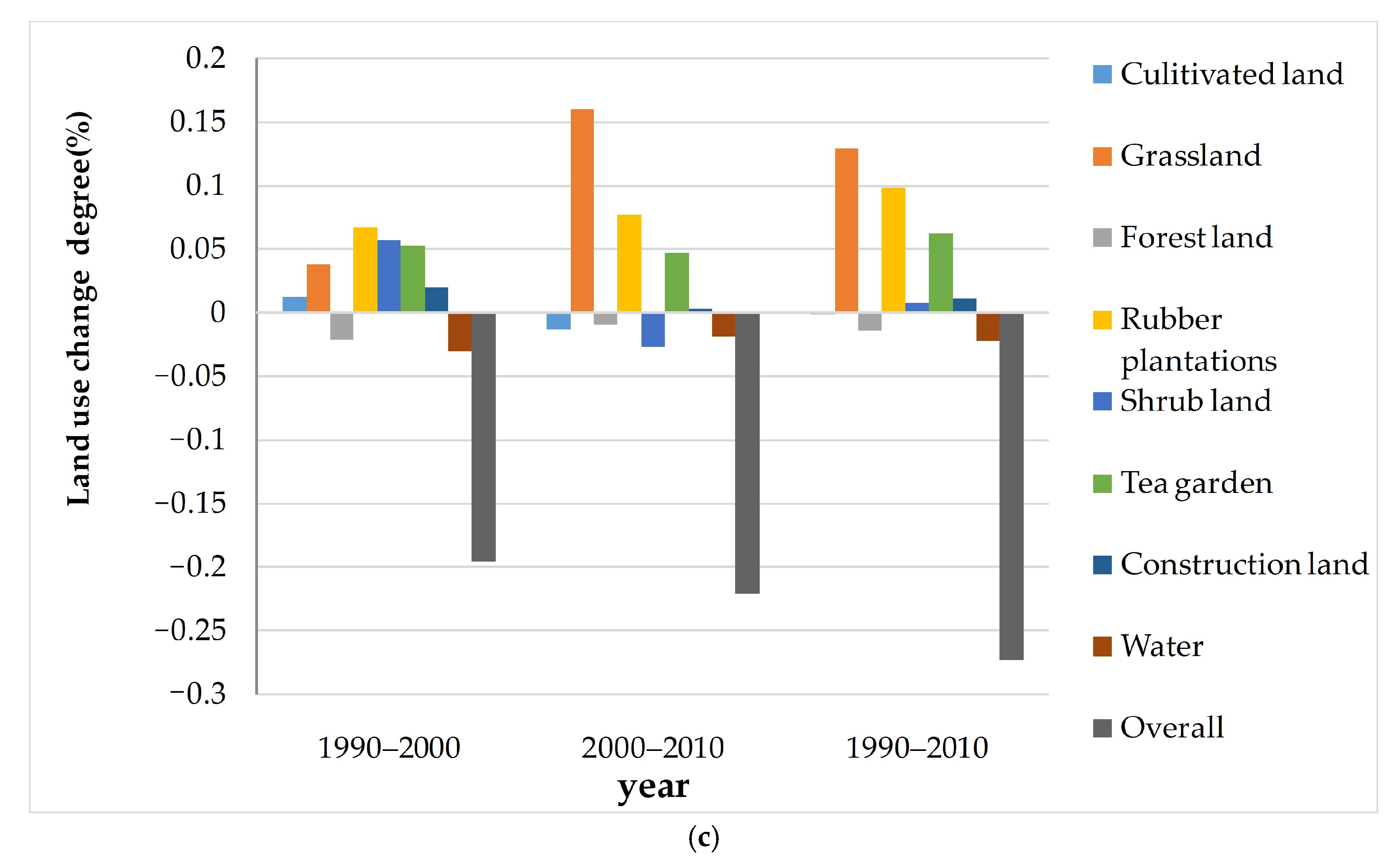
The areas, changes, and dynamics of the three types of land use in 1990, 2000, and 2010 are shown in Figure 4.

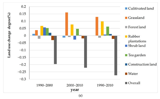
Figure 4.
(a)Land use areas in 1990, 2000, and 2010, (b) changes in land use type, and (c) land use change degree in Xishuangbanna between 1990 to 2000, 2000 to 2010, and 1990 to 2010.
As shown in Figure 4, the areas under cultivated land, forested land, and water bodies in Xishuangbanna showed a downward trend from 1990 to 2010. Among them, the decrease in forest area is the most obvious, with a total reduction of 360,819 ha (360,819 × 104 m2) over the past 20 years, a dynamic land use change degree of −1.42%, a decrease of 265,491 ha (265,491 × 104 m2) from 1990 to 2000, and a reduction of 95,328 ha (95,328 × 104 m2) from 2000 to 2010. The area of cultivated land showed an increasing trend in the previous 10 years, marked by a rise of 18,153 ha (18,153 × 104 m2) and a dynamic land use change degree of 1.24%. The area of cultivated land decreased by a total of 21,456 ha (21,456 × 104 m2) in the latter 10 years, with a dynamic land use change degree of −1.31%. The area under water bodies declined continuously for the two decades, with a total reduction of 3996 ha (3996 × 104 m2) and a dynamic degree of −2.17%. Grasslands, rubber plantations, shrubland, tea gardens, and construction land in Xishuangbanna region showed increasing trends from 1990 to 2010. Among them, the area of rubber plantations showed the most obvious growth, with a total increase of 249,948 ha (249,948 × 104 m2) in 20 years, and a dynamic land use change degree of 9.87%. Moreover, the area under tea gardens increased by 43,686 ha (43,686 × 104 m2) in the past 20 years, the dynamic land use change degree being 6.26%. Although the areas under grassland, shrubland, and construction land increased, the changes were relatively insignificant.
In summary, the economic development of the Xishuangbanna region and the improvement in people’s quality of life led to a rise in the cultivation of cash crops such as rubber and tea in the region in the past 20 years, resulting in a large number of forests being felled.
During the period 1990–2000, carbon emissions for Global Forest Watch and Santoro datasets were 7.85 million t CO2e and 5.63 million t CO2e, respectively, with a difference of 28.30%. During the period 2000–2010, carbon emissions for Global Forest watch and Santoro datasets were 2.82 million t CO2e and 2.00 million t CO2e, respectively, with a difference of 28.81%. Carbon emissions for the period 1990–2000 were about 2.8 times as much as those for the period 2000–2010 (Figure 5).
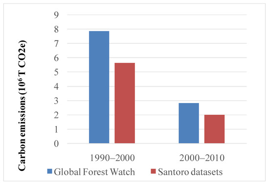
Figure 5.
Carbon emissions for the period 1990–2000 and the period 2000–2010.
3.2. Influencing Factors of Land Use Change
There are many drivers that lead to deforestation and forest degradation within REDD+. Direct drivers are human activities or immediate actions that directly impact forest cover and loss of carbon such as agriculture expansion (both commercial and subsistence), infrastructure extension, and wood extraction. Indirect drivers are complex interactions of social, economic, political, cultural, and technological processes to cause deforestation or forest degradation. They act at multiple scales: international (markets, commodity prices), national (population growth, domestic markets, national policies, governance), and local circumstances (subsistence, poverty) [64,65,66,67]. Since RLs refer to the business-as-usual scenario, which means without any change in REDD+ drivers (situation, government, socio-economic forces, etc. that occur over time), this study only considered seven factors influencing land use change, namely distance to a road, distance to a river, elevation, slope, aspect, distance to an administrative center, and nature reserves (Table 3 and Figure 6).

Table 3.
Factors influencing land use change and data acquisition methods.
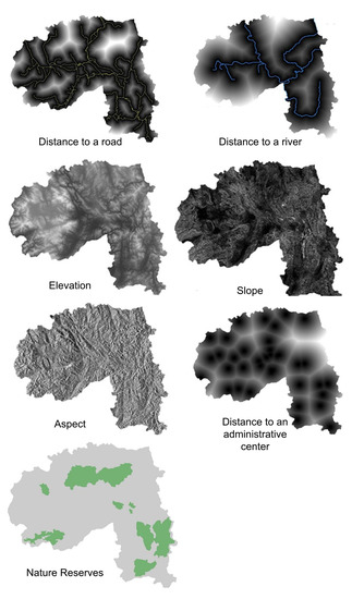
Figure 6.
Influencing factors of land use change in Xishuangbanna region.
Cramer’s V coefficients (Table 4) were calculated to measure the correlation between the above-mentioned factors impacting land use change and land distribution. The larger the value, the stronger the correlation.

Table 4.
Cramer’s V coefficients indicating correlations between the influencing factors of land use change and land distribution.
3.2.1. Distance to a Road
Besides playing a very important role in the economic and social development of a region, traffic conditions impact the land use status of a region. The overall correlation between the land type and distance from a road is 0.1334. Firstly, compared with the overall value, Cramer’s V coefficient for shrubland and tea gardens is 0.2735 and 0.2148, respectively, which is much higher than the overall value. Thus, the distance from a road is a relative important factor affecting shrubland and tea gardens. Secondly, Cramer’s V coefficient of the impact of the distance from a road on rubber plantations and construction land is 0.1550 and 0.1411, respectively, quite similar to the overall value. Thus, the affected land types dominated by road traffic in the Xishuangbanna region are shrubland, tea gardens, rubber plantations, and construction. It is evident that these land types are affected by anthropogenic activity. The reason of highest correlation between the shrubland and road is that it is very common in Xishuanbbanna to have roads built across shrubland rather other areas.
3.2.2. Distance to a River
The precipitation in Xishuangbanna region is abundant and evenly distributed. The dependence of most land use types on rivers is not obvious, except for shrubland and tea gardens. Among them, the influencing factor, namely the overall correlation value of the distance from a river to the land type is 0.0905, and the Cramer’s V coefficients for tea gardens (0.1277) are higher than this overall value. This result indicates that the distance from a river is the main factor affecting tea gardens.
3.2.3. Terrain-Related Factors
Topographic factors play a very important limiting role in various production activities. The study area is mainly mountainous, and, thus, the topographic factors of elevation, slope, and aspect cannot be ignored. Firstly, the overall value of the correlation is 0.2539, and woodland and rubber plantations alone show higher correlation coefficients than this overall value (the corresponding Cramer’s V coefficients are 0.3482 and 0.5297). During the period 1990–2010, the rubber plantation in Xishuangbanna continuously expanded from low-altitude flat valleys to mountainous areas in high altitudes due to high rubber price from the international market, population pressure, and economic development. This is the reason for the highest correlation between the elevation and rubber plantation. Cramer’s V coefficients of elevation for shrubland, grassland, cultivated land, tea gardens, construction land, and other land are 0.1192, 0.1289, 0.1355, 0.1230, 0.0451, and 0.2130, respectively, indicating that their correlation coefficients are lower than the overall value.
Secondly, the slope affects the water distribution, wind speed, and soil texture required for crop growth. The overall value of the correlation for the slope is 0.1608, while Cramer’s V coefficients for shrubland, rubber plantations, and tea gardens are 0.2131, 0.1984, and 0.1665, respectively, higher than the overall value. Thus, this factor can be regarded as the main factor impacting these land uses. However, in overall terms, Cramer’s V coefficient is less than the corresponding values for grassland, cultivated land, construction land, and other land (0.0406, 0.0210, 0.1076, and 0.0256, respectively).
Finally, the aspect primarily affects the length of time and temperature for the growth and final yield of crops. The overall value in this case is 0.0431, while Cramer’s V coefficients for shrubland, grassland, and rubber plantations are all greater than the overall value (0.0729, 0.0560, and 0.0570, respectively).
3.2.4. Distance to an Administrative Center
Governmental administrative organizations are typically located in townships. Given the increasingly strict forest protection policies being applied to Xishuangbanna region, areas closer to governmental administrative organizations can be conveniently supervised and regulated, resulting in a certain deterrent effect on forest destruction and illegal mining of local resources. The overall value of the distance from a township is 0.1252. The corresponding Cramer’s V coefficients for rubber plantations, and tea gardens (0.1542, and 0.1516, respectively) are higher than the overall value. However, the coefficients for grassland, cultivated land, construction land, and other land (namely, 0.0933, 0.0455, 0.1025, and 0.0361, respectively) are less than the overall value. Therefore, rubber plantations and tea gardens are clearly (and expectedly) impacted by distance to a township, whereas this is not so for the remaining land use types.
3.2.5. Limiting Factor (Nature Reserve)
Xishuangbanna Nature Reserve is a national nature reserve consisting of five small sub-reserves, namely the Mengyang, Menglun, Mengla, Shangyong, and Manzhang Reserves. These sub-reserves are not geographically connected to each other and cover a total area of 242,500 ha (242,500 × 104 m2). Notably, 12.68% of the total area of the Prefecture is allocated to nature conservation, namely the protection of the tropical forest ecosystem and its rare wildlife. Relatively little land change has been observed in the protected area, and man-made damage has also been effectively contained. In this study, the conversion rate of certain land use types, such as forestland, in the protected area was set to 0; in other words, anthropogenic activities in these areas are completely restricted.
3.3. Future Land Use Simulation Results and Inspection
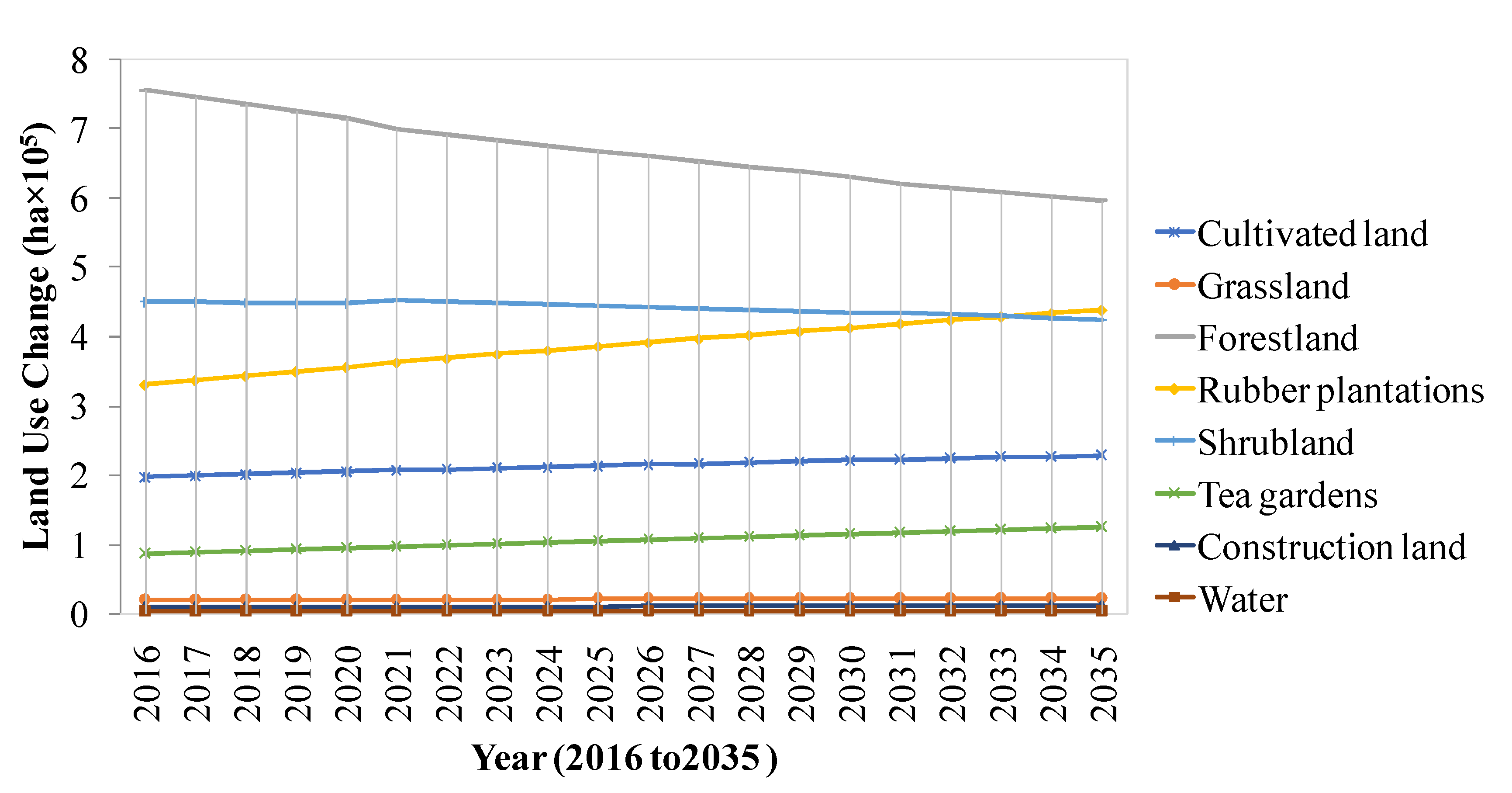
The expansion of rubber and other cash crops has caused massive forest loss and fragmentation in Xishuangbanna. The region experienced the most severe forest losses and degradation particularly for the period 1990 to 2010. Therefore, we chosen the period 1990 to 2010 for REDD+ in Xishuangbanna as the baseline, which is crucial to measure the emission reduction performance and consequently to negotiate meaningful deforestation emission reduction targets. As a result, the land use change data for 1990 and 2000 were used as inputs to the model of the Markov chain and MLP, and the 2010 land use change data were used as the verification values to simulate future land use. The validation of AUC value from the ROC curve method is 0.8, indicating that the results provided by the model are ideal. The land use prediction results for the Xishuangbanna region in the next 20 years of 2016–2035 are shown in Figure 7.
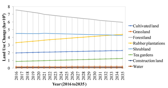
Figure 7.
Land use forecast for Xishuangbanna region for the next 20 years (unit: ha or 104 m2).
Area under forestland shows a downward trend and is the largest change over the 20 years, with the areal reduction amounting to 158,535 ha (158,535 × 104 m2). Conversely, the areas under rubber plantations, tea gardens, and cultivated land increase, with rubber plantations showing the highest increase (by 108,450 ha (108,450 × 104 m2)). The areas under tea gardens and cultivated land also increase, but only slightly (by 39,204 ha (39,204 × 104 m2) and 31,707 ha (31,707 × 104 m2), respectively). The areas under shrubland, grassland, construction land, and water bodies remained stable. Thus, in the next 20 years, the Xishuangbanna region will undergo further deforestation; simultaneously, given its improved economic development and the rising human demand for resources, the cultivation of cash crops such as rubber and tea will continue to increase, which will add pressure on the region’s forests.
3.4. Reference Levels in Xishuangbanna
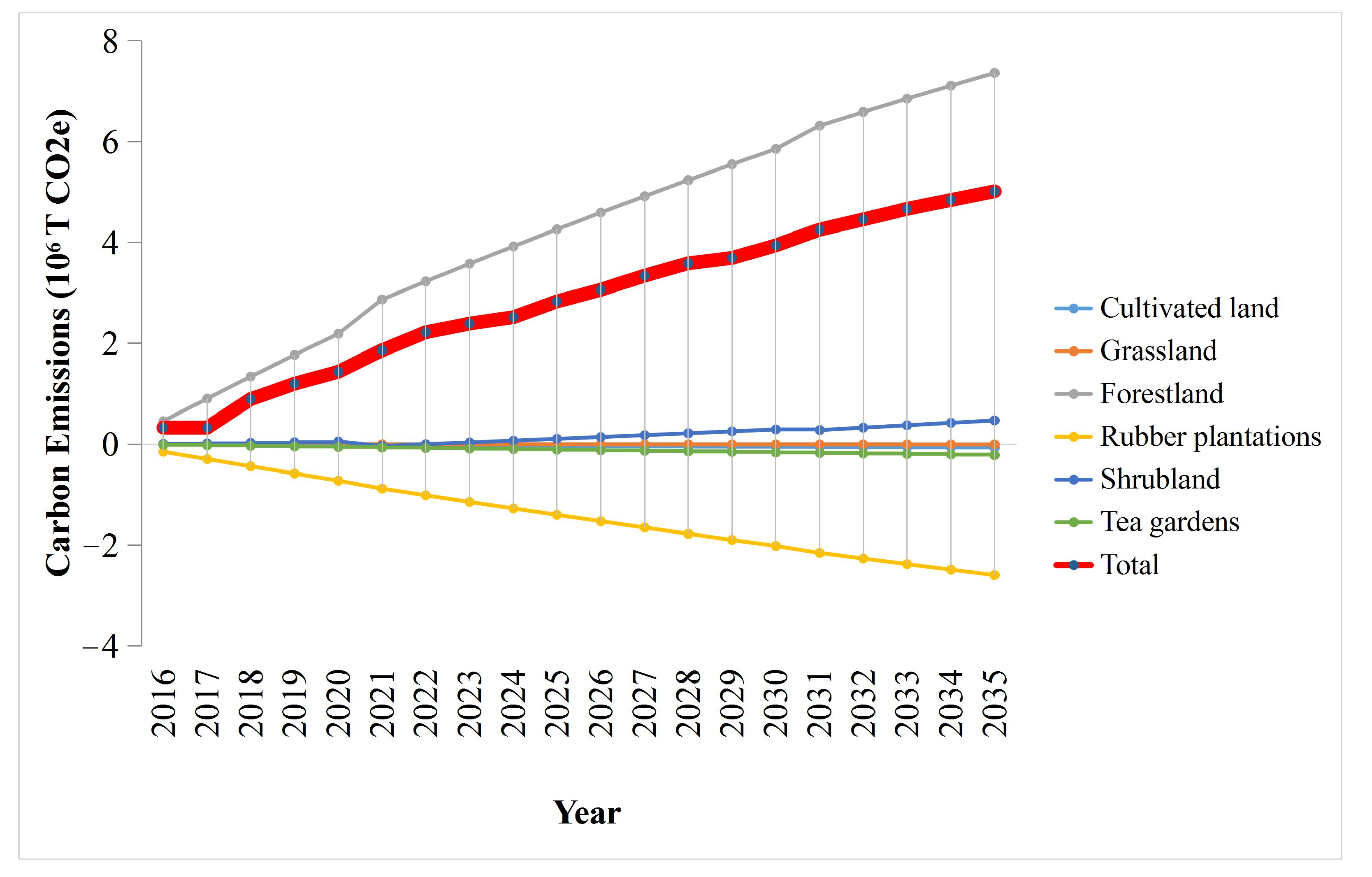
According to IPCC’s Good Practice Guidance, the source/or sink estimates were determined by multiplying the activity data by a carbon stock coefficient (i.e., emission factor) at two points in time. In this study, the combination of the IPCC method and the land use change model showed that the carbon emissions from the study region obviously increased year by year over the 20 years of this study (Figure 8); the simulated growth trend provides an estimate of 0.35 million t CO2e of annual carbon emissions on average. Simultaneously, the large increase in rubber plantations facilitated a rise in carbon absorption, resulting in average annual carbon sequestration of 0.13 million t CO2e. Although the total amount of carbon sequestration attributable to cultivated land, grassland, shrubland, and tea gardens changed, the overall increase was not large. In general, the total carbon emissions in Xishuangbanna rose year by year during the past two decades. The average annual carbon emissions in the past two decades were estimated to be 0.23 million t CO2e, while the total carbon emissions in the same time period amounted to 4.6866 million t CO2e, indicating an obvious increase.
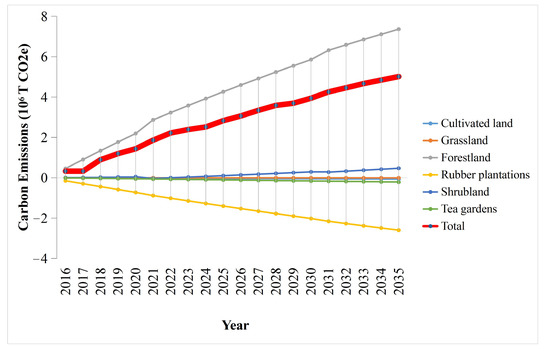
Figure 8.
Reference levels in the Xishuangbanna region.
4. Conclusions
A careful assessment of RLs for REDD+ in Xishuangbanna, China provides significant insights to REDD+ project. The implications that emerge from this study are as follows.
1. We developed a methodological framework to estimate carbon emissions for the REDD+ program in the tropical forests of Xishuangbanna, China. By coupling IPCC’s GPG and land use scenario modeling, we could successfully estimate the RLs. Within the framework, the Enhanced Thematic Mapper Plus/Thematic Mapper(ETM+/TM) remote sensing images in the study area were used to interpret land use changes in 1990, 2000, and 2010. The Land Use Dynamic Index was used for the transfer of land use types during the study period to identify that rubber plantations were the main contributor to forest loss in this region. The Markov chain model was used to predict the number of future land use changes and the Multilayer Perceptron model was applied to calculate the distribution location of these changes.
2. According to Paragraph 71 of Decision 1/CP.16, forests RLs are one of the elements to implement REDD+ activities for developing country parties. Moreover, the COP recognizes the importance and necessity of adequate and predictable financial and technology support for developing such RLs. Identifying these RLs is, therefore, a critical step in the provision of financial incentives and/or creation of carbon markets. Furthermore, they guide the design of the REDD+ strategy. In this study for the business-as-usual scenario of the RLs, Xishuangbanna will lose 158,535 ha (158,535 × 104 m2) of forest area in next 20 years, resulting in approximately 0.23 million t (0.23 × 10⁹ kg) CO2e emissions per year. This is due to the improved economic development and the rising human demand for resources, such as the cultivation of rubber and tea.
5. Future Scope
Estimating carbon emissions based on RLs is a multidisciplinary task. It requires expertise in forestry science, ecological modeling, statistics, remote sensing, and field techniques. Undertaking this exercise is demanding given global geographical diversity, and, thus, building technical capacity to this end is essential. Modeling future emissions based on historical trend rates and understanding the relationships between deforestation patterns and the drivers of deforestation are essential for RL estimation [68,69,70].
Remote sensing technology using optical sensors is capable of measuring the carbon content of different forest types when supported by field information from, for example, sample plots used to calibrate the technology. Using this methodology, a multitemporal set of remotely sensed data can be used to detect forest changes over time [71,72,73]. Thus, freely available Landsat images can provide reliable measurements of forest change, especially when complemented with high-resolution satellite imagery from sensors such as QuickBird, which provide data for image analysis training and validation.
Author Contributions
Conceptualization, H.L.; Data curation, G.L., C.Z. and K.H.; Formal analysis, K.H., Y.F. and M.X.; Investigation, Y.F., M.X. and R.G.; Methodology, G.L. and C.Z.; Project administration, H.L.; Resources, G.L.; Writing—original draft, H.L. and G.L.; Writing—review and editing, H.L. All authors have reviewed and agreed to the published version of the manuscript.
Funding
This study is under the auspices of NSFC42071267, NSFC41371525, Program for Innovative Research Team (in Science and Technology) in University of Henan Province (21IRTSTHN008), Dabieshan National Observation and Research Field Station of Forest Ecosystem at Henan andSYL20060111.
Acknowledgments
We are grateful to Quntao Yang’s contribution to the research. We are also indebted to Liangyun Liu and Bowen Song, our colleagues at the Aerospace Information Research Institute (AIR) under the Chinese Academy of Sciences (CAS), for their kind help on China’s GlobeLand30.
Conflicts of Interest
The authors declare no conflict of interest.
Appendix A

Table A1.
The accuracies in 1990.
Table A1.
The accuracies in 1990.
| Reference Date (1990) | Total | UA | ||||||||
|---|---|---|---|---|---|---|---|---|---|---|
| Classification | Forest Land | Shrub Land | Cultivated Land | Rubber Plantations | Water | GrassLand | Constructionland | Tea Gardens | ||
| Forest land | 1350 | 67 | 0 | 45 | 0 | 30 | 0 | 28 | 1520 | 88.82% |
| Shrub land | 55 | 320 | 11 | 25 | 0 | 13 | 0 | 0 | 424 | 75.47% |
| Cultivated land | 0 | 0 | 245 | 0 | 15 | 0 | 12 | 0 | 272 | 90.07% |
| Rubber plantations | 24 | 12 | 0 | 277 | 0 | 10 | 0 | 0 | 323 | 85.76% |
| Water | 0 | 12 | 0 | 0 | 40 | 13 | 0 | 0 | 65 | 61.54% |
| Grassland | 15 | 0 | 15 | 0 | 0 | 65 | 0 | 0 | 95 | 68.42% |
| Construction land | 0 | 0 | 10 | 0 | 0 | 0 | 45 | 0 | 55 | 81.82% |
| Tea gardens | 0 | 12 | 15 | 11 | 0 | 0 | 0 | 74 | 112 | 66.07% |
| Total | 1444 | 423 | 296 | 358 | 55 | 131 | 57 | 102 | 2866 | |
| PA | 93.49% | 75.65% | 82.77% | 77.37% | 72.73% | 49.62% | 78.95% | 72.55% | OA = 84.30% | |
| Omissionerror | 0.065 | 0.243 | 0.172 | 0.226 | 0.273 | 0.504 | 0.211 | 0.275 | Kappa = 0.770 | |
| Commission error | 0.120 | 0.043 | 0.012 | 0.018 | 0.009 | 0.011 | 0.004 | 0.014 | ||

Table A2.
The accuracies in 2000.
Table A2.
The accuracies in 2000.
| Reference Date (2000) | Total | UA | ||||||||
|---|---|---|---|---|---|---|---|---|---|---|
| Classification | Forest Land | Shrub Land | Cultivated Land | Rubber Plantations | Water | Grassland | Constructionland | Tea Gardens | ||
| Forest land | 1100 | 54 | 20 | 31 | 0 | 0 | 0 | 22 | 1227 | 89.65% |
| Shrub land | 27 | 385 | 0 | 29 | 0 | 15 | 0 | 0 | 456 | 84.43% |
| Cultivated land | 0 | 0 | 260 | 0 | 15 | 0 | 11 | 0 | 289 | 90.91% |
| Rubber plantations | 15 | 12 | 0 | 163 | 0 | 10 | 0 | 0 | 200 | 81.50% |
| Water | 0 | 12 | 0 | 0 | 30 | 13 | 0 | 0 | 55 | 54.55% |
| Grassland | 0 | 0 | 15 | 0 | 0 | 57 | 0 | 0 | 72 | 79.17% |
| Construction land | 0 | 0 | 14 | 0 | 0 | 0 | 45 | 0 | 59 | 76.27% |
| Tea garden | 0 | 11 | 0 | 13 | 0 | 0 | 0 | 80 | 104 | 76.92% |
| Total | 1142 | 474 | 309 | 236 | 45 | 95 | 56 | 102 | 2459 | |
| PA | 96.32% | 81.22% | 84.14% | 69.07% | 66.67% | 60.00% | 80.36% | 78.43% | OA = 86.21% | |
| Omission error | 0.037 | 0.188 | 0.159 | 0.309 | 0.333 | 0.400 | 0.196 | 0.216 | Kappa = 0.805 | |
| Commission error | 0.096 | 0.036 | 0.014 | 0.017 | 0.010 | 0.006 | 0.006 | 0.010 | ||

Table A3.
The accuracies in 2010.
Table A3.
The accuracies in 2010.
| Reference Date (2010) | Total | UA | ||||||||
|---|---|---|---|---|---|---|---|---|---|---|
| Classification | Forest Land | Shrub Land | Cultivated Land | Rubber Plantations | Water | Grassland | Constructionland | Tea Gardens | ||
| Forest land | 856 | 54 | 0 | 45 | 0 | 25 | 0 | 28 | 1008 | 84.92% |
| Shrub land | 16 | 275 | 15 | 25 | 0 | 0 | 0 | 0 | 331 | 83.08% |
| Cultivated land | 0 | 0 | 245 | 0 | 15 | 0 | 12 | 0 | 272 | 90.07% |
| Rubber plantations | 38 | 12 | 0 | 390 | 0 | 10 | 0 | 0 | 450 | 86.67% |
| Water | 0 | 14 | 0 | 0 | 40 | 0 | 0 | 0 | 54 | 74.07% |
| Grassland | 20 | 0 | 25 | 0 | 0 | 80 | 0 | 0 | 125 | 64.00% |
| Construction land | 0 | 0 | 14 | 0 | 0 | 0 | 45 | 0 | 59 | 76.72% |
| Tea gardens | 0 | 20 | 17 | 13 | 0 | 0 | 0 | 132 | 182 | 72.53 % |
| Total | 930 | 375 | 316 | 473 | 55 | 115 | 57 | 160 | 2481 | |
| PA | 92.04% | 77.33% | 77.53% | 82.45% | 72.73% | 69.57% | 78.95% | 82.50% | OA = 83.15% | |
| Omission error | 0.080 | 0.267 | 0.225 | 0.175 | 0.273 | 0.304 | 0.211 | 0.175 | Kappa = 0.781 | |
| Commission error | 0.098 | 0.027 | 0.014 | 0.030 | 0.006 | 0.019 | 0.006 | 0.022 | ||
References
- FAO. Global Forest Resource Assessment 2005; FAO: Rome, Italy, 2006. [Google Scholar]
- Baccini, A.; Walker, W.; Carvalho, L.; Farina, M.; Sulla-Menashe, D.; Houghton, R.A. Tropical forests are a net carbon source based on aboveground measurements of gain and loss. Science 2017, 358, 230–234. [Google Scholar] [CrossRef] [PubMed]
- Hubau, W.; Lewis, S.; Phillips, O.; Affum-Baffoe, K.; Beeckman, H.; Cuní-Sanchez, A.; Daniels, A.K.; Ewango, C.E.N.; Fauset, S.; Mukinzi, J.M.; et al. Asynchronous Carbon Sink Saturation in African and Amazonian Tropical Forests. Nature 2020, 579, 80–87. [Google Scholar] [CrossRef] [PubMed]
- Sagar, R.; Li, G.; Singh, J.S.; Wan, S. Carbon fluxes and species diversity in grazed and fenced typical steppe grassland of Inner Mongolia, China. J. Plant Ecol. 2019, 12, 10–22. [Google Scholar] [CrossRef]
- Lu, H.; Liu, G.; Zhang, C.; Okuda, T. Approaches to quantifying carbon emissions from degradation in pan-tropic forests—Implications for effective REDD monitoring. Land Degrad. Dev. 2020, 31, 1890–1905. [Google Scholar] [CrossRef]
- Barbier, E.B.; Lozano, R.; Rodríguez, C.M.; Troëng, S. Adopt a carbon tax to protect tropical forests. Nature 2020, 578, 213–216. [Google Scholar] [CrossRef]
- Tagesson, T.; Schurgers, G.; Horion, S.; Ciais, P.; Tian, F.; Brandt, M.; Ahlström, A.; Wigneron, J.P.; Ardö, J.; Olin, S.; et al. Recent divergence in the contributions of tropical and boreal forests to the terrestrial carbon sink. Nat. Ecol. Evol. 2020, 4, 202–209. [Google Scholar] [CrossRef] [PubMed]
- Hansen, M.C.; Potapov, P.; Tyukavina, A. Comment on “Tropical forests are a net carbon source based on aboveground measurements of gain and loss”. Science 2019, 363, eaar3629. [Google Scholar] [CrossRef]
- Melillo, J.M.; McGuire, A.D.; Kicklighter, D.W.; Moore, B.; Vorosmarty, C.J.; Schloss, A.L. Global climate change and terrestrial net primary production. Nature 1993, 363, 234–240. [Google Scholar] [CrossRef]
- Liu, G.; Liu, Q.; Song, M.; Chen, J.; Zhang, C.; Meng, X.; Zhao, J.; Lu, H. Costs and Carbon Sequestration Assessment for REDD+ in Indonesia. Forests 2020, 11, 770. [Google Scholar] [CrossRef]
- Lin, D.; Xia, J.; Wan, S. Climate warming and biomass accumulation of terrestrial plants: A meta-analysis. New Phytol. 2010, 188, 187–198. [Google Scholar] [CrossRef]
- Liang, J.; Xia, J.; Liu, L.; Wan, S. Global patterns of the responses of leaf-level photosynthesis and respiration in terrestrial plants to experimental warming. J. Plant Ecol. 2013, 6, 437–447. [Google Scholar] [CrossRef]
- Wang, H.; Chen, W. Modeling of energy transformation pathways under current policies, NDCs and enhanced NDCs to achieve 2-degree target. Appl. Energy 2019, 250, 549–557. [Google Scholar] [CrossRef]
- Marx, A.; Kumar, R.; Thober, S.; Zink, M.; Wanders, N.; Wood, E.; Pan, M.; Sheffield, J.; Samaniego, L. Climate change alters low flows in Europe under a 1.5, 2, and 3 degree global warming. Hydrol. Earth Syst. Sci. Discuss. 2017, 22, 1017–1032. [Google Scholar] [CrossRef]
- Ha, Y.; Teng, F. Midway toward the 2 degree target: Adequacy and fairness of the Cancun pledges. Appl. Energy 2013, 112, 856–865. [Google Scholar] [CrossRef]
- Meinshausen, M.; Meinshausen, N.; Hare, W.; Raper, S.C.B.; Frieler, K.; Knutti, R.; Frame, D.J.; Allen, M.R. Greenhouse-gas emission targets for limiting global warming to 2 C. Nature 2009, 458, 1158–1162. [Google Scholar] [CrossRef]
- Roopsind, A.; Sohngen, B.; Brandt, J. Evidence that a national REDD+ program reduces tree cover loss and carbon emissions in a high forest cover, low deforestation country. Proc. Natl. Acad. Sci. USA 2019, 116, 24492–24499. [Google Scholar] [CrossRef]
- Sheng, J.; Qiu, H. Governmentality within REDD+: Optimizing incentives and efforts to reduce emissions from deforestation and degradation. Land Use Policy 2018, 78, 611–622. [Google Scholar] [CrossRef]
- Seymour, F.; Boyd, W.; Stickler, C.; Duchelle, A.E.; Nepstad, D.; Bahar, N.H.A.; Rodriguez-Ward, D. Jurisdictional Approaches to REDD+ and Low Emissions Development: Progress and Prospects; World Resources Institute: Washington, WA, USA, 2018. [Google Scholar]
- Johnson, B.A.; Scheyvens, H.; Samejima, H. Quantitative Assessment of the Earth Observation Data and Methods Used to Generate Reference Emission Levels for REDD+. In Satellite Earth Observations and Their Impact on Society and Policy; Onoda, M., Young, O.R., Eds.; Springer: Singapore, 2017. [Google Scholar]
- Johnson, B.A.; Scheyvens, H.; Samejima, H.; Onoda, M. Characteristics of the remote sensing data used in the proposed UNFCCC REDD+ forest reference emission levels (FRELs). ISPRSInt. Arch. Photogramm. Remote Sens. Spat. Inf. Sci. 2016, 8, 669–672. [Google Scholar] [CrossRef]
- Reimer, F.; Asner, G.P.; Joseph, S. Advancing reference emission levels in subnational and national REDD+ initiatives: A CLASlite approach. Carbon Balance Manag. 2015, 10, 5. [Google Scholar] [CrossRef]
- Herold, M.; Achard, F.; DeFries, R.; Skole, D.; Brown, S.; Townshend, J. Report of the workshop on monitoring tropical deforestation for compensated reductions. In Proceedings of the GOFC-GOLD Symposium on Forest and Land Cover Observations, Jena, Germany, 21–22 March 2006. [Google Scholar]
- Lu, H.; Liu, G. Opportunity Costs of Carbon Emissions Stemming from Changes in Land Use. Sustainability 2015, 7, 3665–3682. [Google Scholar] [CrossRef]
- Lu, H.; Liu, G.; Huang, Z.; Yang, Q. Carbon, soil, and ecological benefits of REDD+ policies in Southwest China. Sci. Asia 2016, 42, 1–11. [Google Scholar] [CrossRef][Green Version]
- Romijn, E.; Ainembabazi, J.H.; Wijaya, A.; Herold, M.; Angelsen, A.; Verchot, L.; Murdiyarso, D. Exploring different forest definitions and their impact on developing REDD+ reference emission levels: A case study for Indonesia. Environ. Sci. Policy 2013, 33, 246–259. [Google Scholar] [CrossRef]
- Bond, I.; Gran, G.M.; Kanounnikoff, W.S.; Hazlewood, P.; Wunder, S.; Angelsen, A. Incentives to Sustain Forest Ecosystem Services: A Review and Lessons for REDD. Natural Resource Issues No. 16; International Institute for Environment &Development: London, UK, 2009. [Google Scholar]
- Hoff, R.; Rajão, R.; Leroy, P. Can REDD+ still become a market? Ruptured dependencies and market logics for emission reductions in Brazil. Ecol. Econ. 2019, 161, 121–129. [Google Scholar] [CrossRef]
- Sukma, M.F. LatarbelakangbantuanJepangterhadap Indonesia melaluimekanisme Reducing Emission from Deforestation and Forest Degradation (REDD+) Tahun. Bachelor’s Thesis, FakultasIlmuSosial dan IlmuPolitik UIN SyarifHidayatullah, Jakarta, Indonesia, March 2018. [Google Scholar]
- Hamdan, O. Forest Reference Emission Level For. REDD+ In Pahang, Malaysia (Research Pamphlet No. 141); Forest Research Institute Malaysia: Kepong, Malaysia, 2018. [Google Scholar]
- Ye, L.; Karunarathna, S.C.; Li, H.; Xu, J.; Hyde, K.D.; Mortimer, P.E. A Survey of Termitomyces (Lyophyllaceae, Agaricales), Including a New Species, from a Subtropical Forest in Xishuangbanna, China. Mycobiology 2019, 47, 391–400. [Google Scholar] [CrossRef] [PubMed]
- Mani, S.; Cao, M. Nitrogen and Phosphorus Concentration in Leaf Litter and Soil in Xishuangbanna Tropical Forests: Does Precipitation Limitation Matter? Forests 2019, 10, 242. [Google Scholar] [CrossRef]
- Li, S.H.; Wang, S.J.; Zhang, Z.; Chen, M.K.; Cao, R.; Cao, Q.B.; Zuo, Q.Q.; Wang, P. Effects of ant nesting on the spatiotemporal dynamics of soil easily oxidized organic carbon in Xishuangbanna tropical forests, China. J. Appl. Ecol. 2019, 30, 413–419. [Google Scholar]
- Goldberg, S.D.; Zhao, Y.; Harrison, R.D.; Monkai, J.; Li, Y.; Chau, K.; Xu, J. Soil respiration in sloping rubber plantations and tropical natural forests in Xishuangbanna, China. Agric. Ecosyst. Environ. 2017, 249, 237–246. [Google Scholar] [CrossRef]
- Marziliano, P.; Veltri, A.; Menguzzato, G.; Pellicone, G.; Coletta, V. A comparative study between “Default Method” And “Stock Change Method” of Good Practice Guidance for Land Use, Land-Use Change and Forestry (IPCC, 2003) to evaluate carbon stock changes in Forest. In Proceedings of the Second International Congress of Silviculture, Florence, Italy, 26–29 November 2014; pp. 551–557. [Google Scholar]
- Grassi, G.; Ravindranath, N.H.; Böttcher, H.; Elhassan, N.; Elsiddig, E.; House, J.I.; Matsumoto, M.; Ometto, J.P.; Sanquetta, C.; Searson, M.J.; et al. Afforestation, Reforestation, Deforestation. In IPCC 2013 Revised Supplementary Methods and Good Practice Guidance Arising from the Kyoto Protocol (KP Supplement); Hiraishi, T., Krug, T., Tanabe, K., Srivastava, N., Jamsranjav, B., Fukuda, M., Troxler, T., Eds.; Institute for Global Environmental Strategies: Kitakyushu, Japan, 2014. [Google Scholar]
- Ohgita, T. Results and Impressions of Expert Meetings for the Preparation of the IPCC Good Practice Guidance. J. Jpn. Soc. Saf. Eng. 2000, 39, 334–342. [Google Scholar]
- Thind, M.P.S.; Wilson, E.J.; Azevedo, I.M.L.; Marshall, J.D. Marginal Emissions Factors for Electricity Generation in the Midcontinent ISO. Environ. Sci. Technol. 2017, 51, 14445–14452. [Google Scholar] [CrossRef]
- Wolf, J.; Asrar, G.R.; West, T.O. Revised methane emissions factors and spatially distributed annual carbon fluxes for global livestock. Carbon BalanceManag. 2017, 12, 16. [Google Scholar] [CrossRef]
- Li, A.; Zhang, A.; Zhou, Y.; Yao, X. Decomposition analysis of factors affecting carbon dioxide emissions across provinces in China. J. Clean. Prod. 2017, 141, 1428–1444. [Google Scholar] [CrossRef]
- MacDicken, K. A Guide to Monitoring Carbon Storage in Forestry and Agroforestry Projects; Winrock International Institute for Agricultural Development: Arlington, VA, USA, 1997. [Google Scholar]
- Brown, S. Measuring carbon in forests: Current status and future challenges. Environ. Pollut. 2002, 116, 363–372. [Google Scholar] [CrossRef]
- Baccini, A.; Goetz, S.J.; Walker, W.S.; Laporte, N.T.; Sun, M.; Sulla-Menashe, D.; Hackler, J.; Beck, P.S.A.; Dubayah, R.; Friedl, M.A.; et al. Estimated carbon dioxide emissions from tropical deforestation improved by carbon-density maps. Nat. Clim. Chang. 2012, 2, 182–185. [Google Scholar] [CrossRef]
- Santoro, M.; Cartus, O.; Carvalhais, N.; Rozendaal, D.; Avitabilie, V.; Araza, A.; Veiga, P.R. The global forest above-ground biomass pool for 2010 estimated from high-resolution satellite observations. Earth Syst. Sci. Data Discuss. 2020. [Google Scholar] [CrossRef]
- Anaya, J.A.; Gutiérrez-Vélez, V.H.; Pacheco-Pascagaza, A.M.; Palomino-Ángel, S.; Han, N.; Balzter, H. Drivers of Forest Loss in a Megadiverse Hotspot on the Pacific Coast of Colombia. Remote Sens. 2020, 12, 1235. [Google Scholar] [CrossRef]
- Sarzynski, T.; Giam, X.; Carrasco, L.; Lee, J.S.H. Combining Radar and Optical Imagery to Map Oil Palm Plantations in Sumatra, Indonesia, Using the Google Earth Engine. Remote Sens. 2020, 12, 1220. [Google Scholar] [CrossRef]
- De Bem, P.P.; De Carvalho Junior, O.A.; Fontes Guimarães, R.; Trancoso Gomes, R.A. Change Detection of Deforestation in the Brazilian Amazon Using Landsat Data and Convolutional Neural Networks. Remote Sens. 2020, 12, 901. [Google Scholar] [CrossRef]
- DeFries, R.; Achard, F.; Brown, S.; Herold, M.; Murdiyarso, D.; Schlamadinger, B.; Souza, C. Reducing Greenhouse Gas Emissions from Deforestation in Developing Countries: Considerations for Monitoring and Measuring; Global Terrestrial Observing System: Rome, Italy, 2006. [Google Scholar]
- Achard, F.; DeFries, R.; Herold, M.; Mollicone, D.; Pandey, D.; de Souza, C. Guidance on monitoring of gross changes in forest area. In Reducing Greenhouse Gas Emissions from Deforestation and Degradation in Developing Countries: A Sourcebook of Methods and Procedures for Monitoring, Measuring and Reporting; Global Observation for Forest Cover and Land Dynamics: Alberta, AB, Canada, 2008. [Google Scholar]
- Wang, X.; Bao, Y. Study on the methods of land use dynamic change research. Prog. Geogr. 1999, 18, 81–87. [Google Scholar]
- Gupta, R.; Sharma, L.K. Efficacy of Spatial Land Change Modeler as a forecasting indicator for anthropogenic change dynamics over five decades: A case study of Shoolpaneshwar Wildlife Sanctuary, Gujarat, India. Ecol. Indic. 2020, 112, 106171. [Google Scholar] [CrossRef]
- Anand, J.; Gosain, A.K.; Khosa, R. Prediction of land use changes based on Land Change Modeler and attribution of changes in the water balance of Ganga basin to land use change using the SWAT model. Sci.Total Environ. 2018, 644, 503–519. [Google Scholar] [CrossRef]
- Jahanifar, K.; Amirnejad, H.; Mojaverian, M.; Azadi, H. Land Change Detection and Identification of Effective Factors on Forest Land Use Changes: Application of Land Change Modeler and Multiple Linear Regression. Eur. Online J. Nat. Soc. Sci. 2018, 7, 554–565. [Google Scholar]
- Mohamed, A.; Worku, H. Simulating urban land use and cover dynamics using cellular automata and Markov chain approach in Addis Ababa and the surrounding. Urban Clim. 2020, 31, 100545. [Google Scholar] [CrossRef]
- Satya, B.A.; Shashi, M.; Deva, P. Future land use land cover scenario simulation using open source GIS for the city of Warangal, Telangana, India. Appl. Geomat. 2020, 12, 281–290. [Google Scholar] [CrossRef]
- Shen, L.; Li, J.; Wheate, R.; Yin, J.; Paul, S.S. Multi-Layer Perceptron Neural Network and Markov Chain Based Geospatial Analysis of Land Use and Land Cover Change. J. Environ. Inform. Lett. 2020, 3, 29–39. [Google Scholar] [CrossRef]
- Kussul, N.; Lavreniuk, M.; Skakun, S.; Shelestov, A. Deep Learning Classification of Land Cover and Crop Types Using Remote Sensing Data. IEEE Geosci. Remote Sens. Lett. 2017, 14, 778–782. [Google Scholar] [CrossRef]
- Ozturk, D. Urban Growth Simulation of Atakum (Samsun, Turkey) Using Cellular Automata-Markov Chain and Multi-Layer Perceptron-Markov Chain Models. Remote Sens. 2015, 7, 5918–5950. [Google Scholar] [CrossRef]
- Cheong, Y.L.; Leitão, P.; Lakes, T. Assessment of land use factors associated with dengue cases in Malaysia using Boosted Regression Trees. Spat. Spatio-Temporal Epidemiol. 2014, 10, 75–84. [Google Scholar] [CrossRef]
- Tien Bui, D.; Shahabi, H.; Shirzadi, A.; Chapi, K.; Pradhan, B.; Chen, W.; Khosravi, K.; Panahi, M.; Bin Ahmad, B.; Saro, L. Land Subsidence Susceptibility Mapping in South Korea Using Machine Learning Algorithms. Sensors 2018, 18, 2464. [Google Scholar] [CrossRef]
- Ghorbanzadeh, O.; Blaschke, T.; Aryal, J.; Gholamnia, K. A new GIS-based technique using an adaptive neuro-fuzzy inference system for land subsidence susceptibility mapping. J. Spat. Sci. 2018, 94, 1–17. [Google Scholar] [CrossRef]
- Chen, J.; Cao, X.; Peng, S.; Ren, H. Analysis and Applications of GlobeLand30: A Review. ISPRS Int. J. Geo-Inf. 2017, 6, 230. [Google Scholar] [CrossRef]
- Xu, C.; Chen, J.; Wu, H.; Li, R.; Zhao, Y.J. An improved pixel counting method for arbitrary zonal statistics on globeland30. ISPRS Int. Arch. Photogramm. Remote Sens. Spat. Inf. Sci. 2019, XLII-4/W20, 101–103. [Google Scholar] [CrossRef]
- Siyum, Z.G. Tropical dry forest dynamics in the context of climate change: Syntheses of drivers, gaps, and management perspectives. Ecol. Process. 2020, 9, 25. [Google Scholar] [CrossRef]
- Geist, H.; Lambin, E. What drives tropical deforestation? A meta-analysis of proximate and underlying causes of deforestation based on subnational case study evidence. Land-Use and Land-Cover Change Project, International Geosphere-Biosphere Programme. LUCC Rep. Ser. 2002, 52, 4. [Google Scholar]
- Geist, H.; Lambin, E. Proximate causes and underlying driving forces of tropical deforestation. BioScience 2002, 52, 143–150. [Google Scholar] [CrossRef]
- Obersteiner, M.; Huettner, M.M.; Kraxner, F.; McCallum, I.; Aoki, K.; Bottcher, H.; Fritz, S.; Gusti, M.; Havlik, P.; Reyers, B.; et al. On fair, effective and efficient REDD mechanism design. Carbon Balance Manag. 2009, 4, 11. [Google Scholar] [CrossRef]
- Ellis, E.A.; Sierra-Huelsz, J.A.; Ceballos, G.C.O.; Binnqüist, C.L.; Cerdán, C.R. Mixed Effectiveness of REDD+ Subnational Initiatives after 10 Years of Interventions on the Yucatan Peninsula, Mexico. Forests 2020, 11, 1005. [Google Scholar] [CrossRef]
- Maraseni, T.N.; Poudyal, B.H.; Rana, E.; Khanal, S.C.; Ghimire, P.L.; Subedi, B.P. Mapping national REDD+ initiatives in the Asia-Pacific region. J. Environ. Manag. 2020, 269, 110763. [Google Scholar] [CrossRef]
- Gallo, P.; Brites, A.; Micheletti, T. REDD+ Achievements and Challenges in Brazil: Perceptions over time (2015-2019); CIFOR: Bogor City, Indonesia, 2020. [Google Scholar]
- Gebhardt, S.; Wehrmann, T.; Ruiz, M.A.M.; Maeda, P.; Bishop, J.; Schramm, M.; Ressl, R. MAD-MEX: Automatic Wall-to-Wall Land Cover Monitoring for the Mexican REDD-MRV Program Using All Landsat Data. Remote Sens. 2014, 5, 3923–3943. [Google Scholar] [CrossRef]
- Mitchell, A.L.; Rosenqvist, A.; Mora, B. Current remote sensing approaches to monitoring forest degradation in support of countries measurement, reporting and verification systems for REDD+. Carbon Balance Manag. 2017, 12, 9. [Google Scholar] [CrossRef]
- Fry, B.P. Community forest monitoring in REDD+: The ‘M’ in MRV? Environ. Sci. Policy 2011, 2, 181–187. [Google Scholar]
Publisher’s Note: MDPI stays neutral with regard to jurisdictional claims in published maps and institutional affiliations. |
© 2021 by the authors. Licensee MDPI, Basel, Switzerland. This article is an open access article distributed under the terms and conditions of the Creative Commons Attribution (CC BY) license (http://creativecommons.org/licenses/by/4.0/).


