The Status of Air Quality in the United States During the COVID-19 Pandemic: A Remote Sensing Perspective


Abstract
1. Introduction
2. Methodology
2.1. Traffic Volume and COVID-19 Cases
2.2. Remote Sensing Products
2.2.1. Nitrogen Dioxide (NO2)
2.2.2. Carbon Monoxide (CO)
2.2.3. Aerosol Optical Depth (AOD)
2.2.4. Tropospheric Ozone Column (O3)
2.3. Analysis Period and Data Significance
2.3.1. Analysis Period
2.3.2. Data Significance
3. Results and Discussion
3.1. Traffic Volume and COVID-19 Cases in the US
3.2. An Overview of Air Quality Tracers in the US
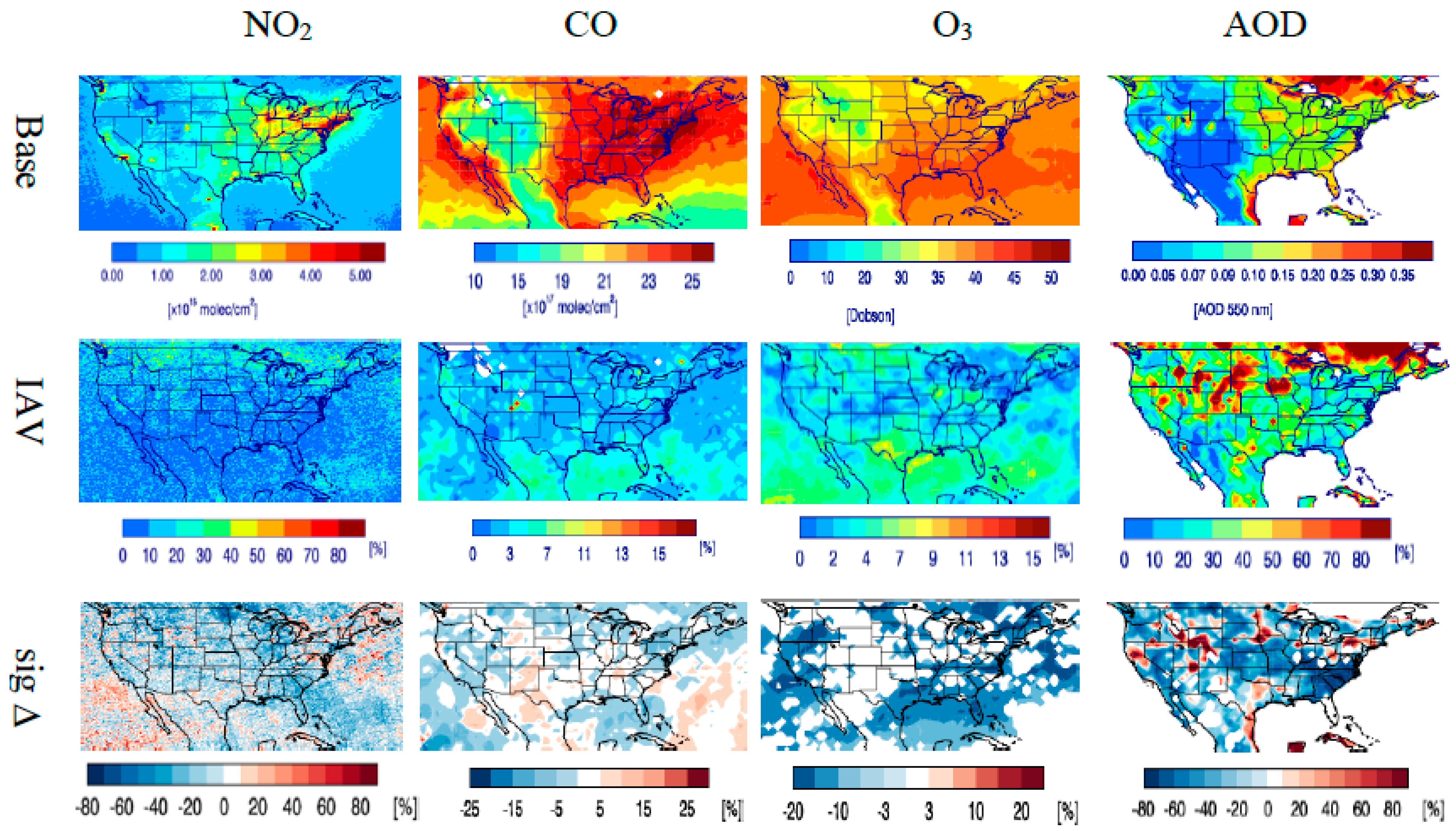
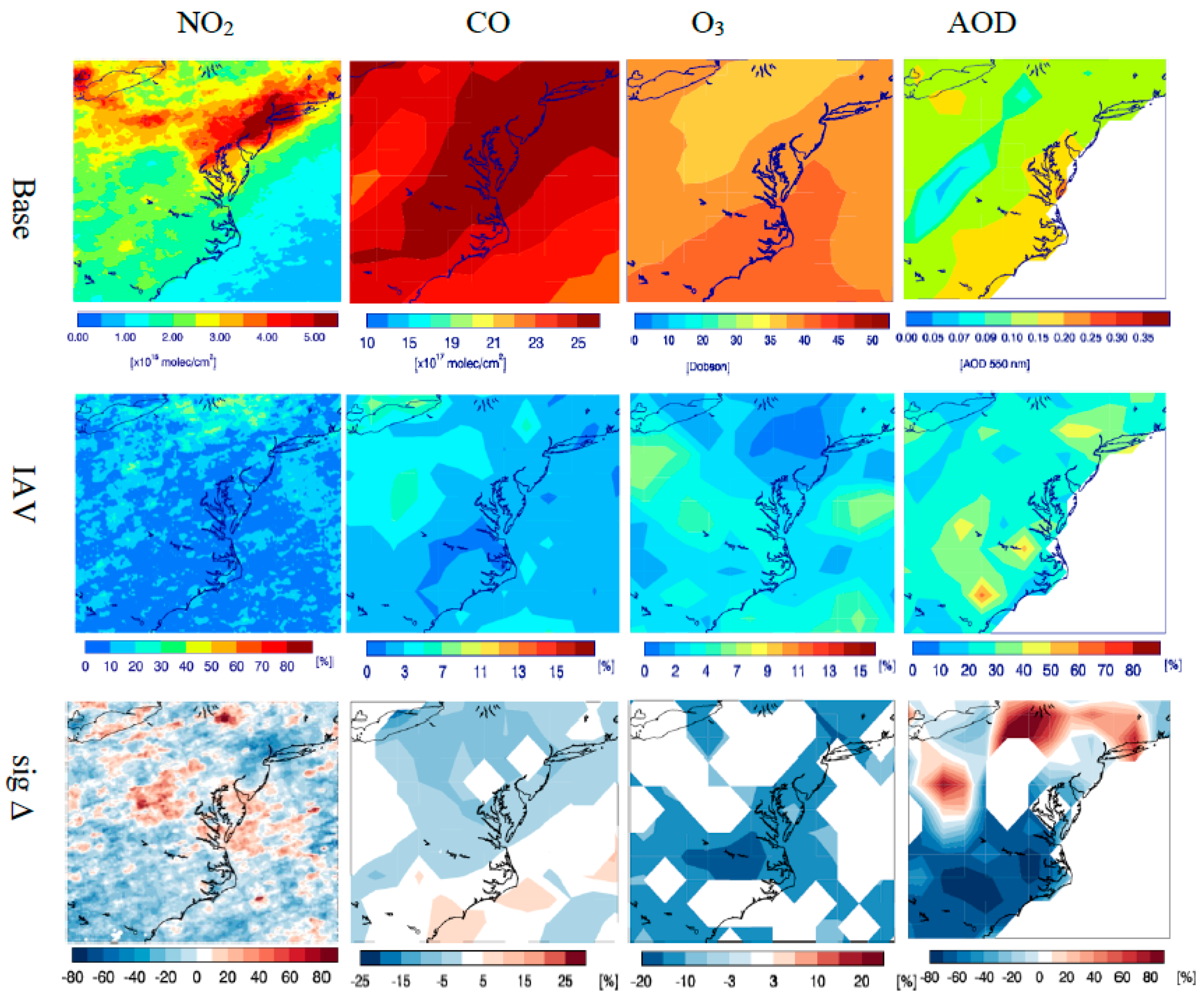
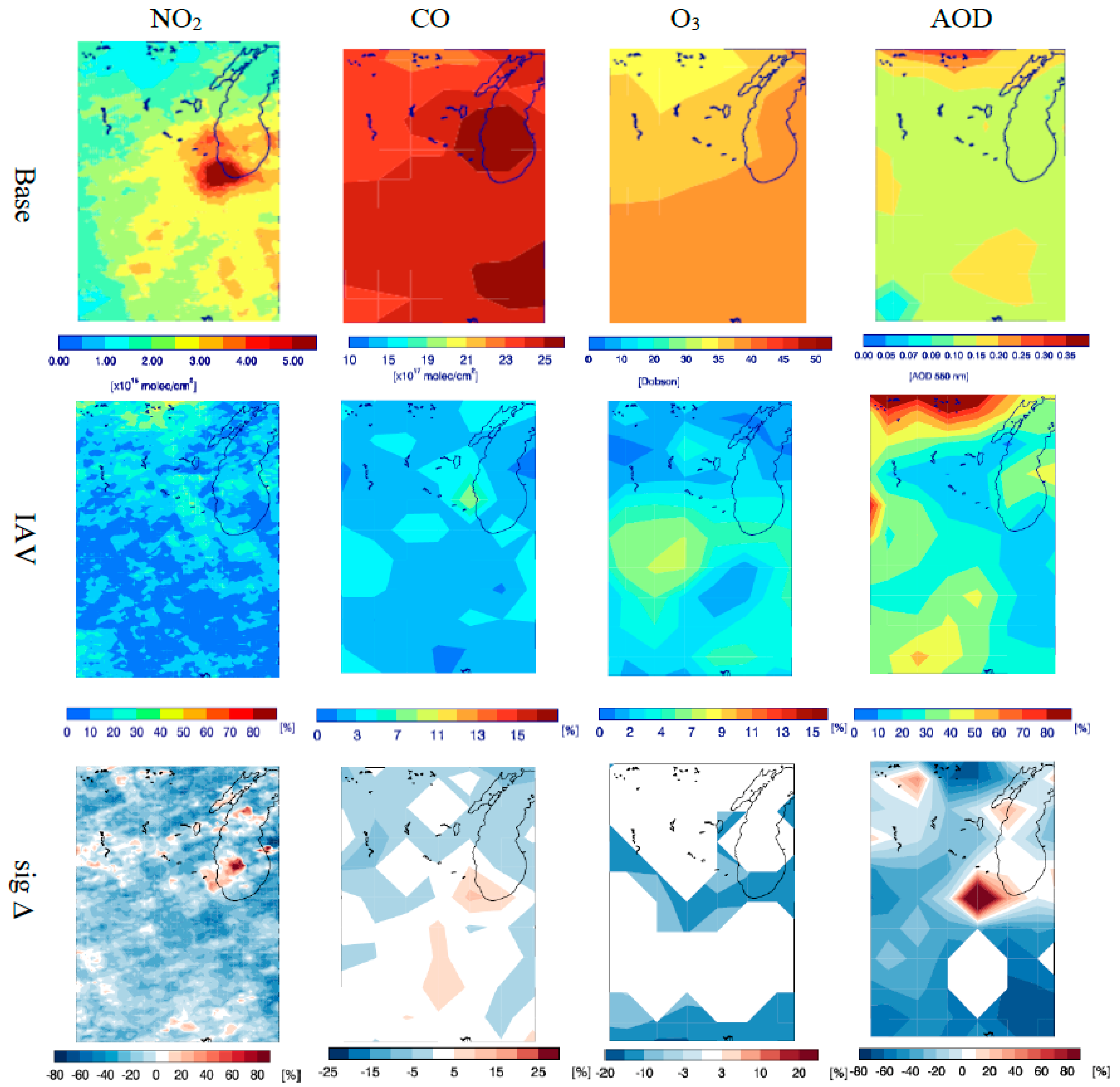
3.2.1. Spatial Distribution
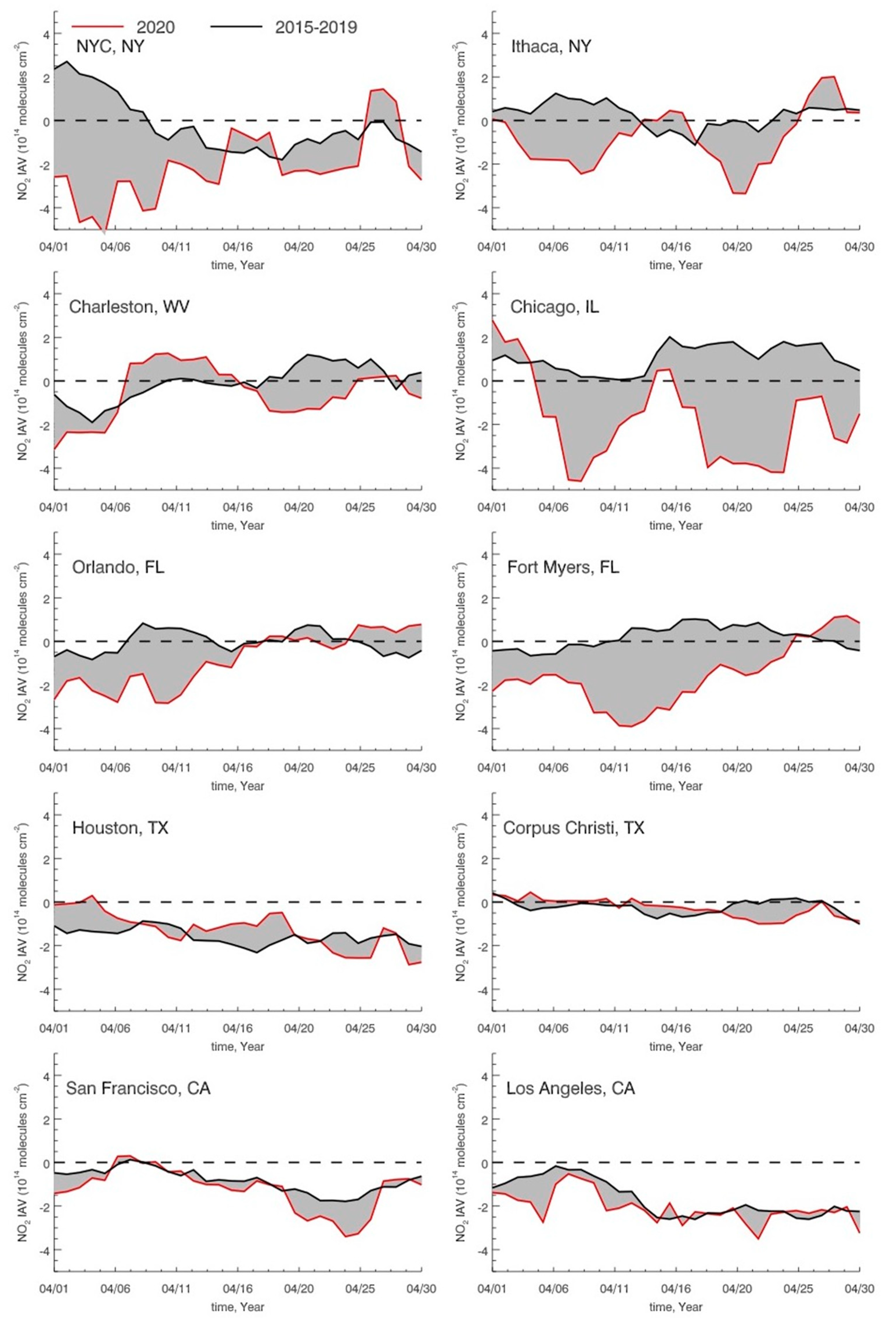
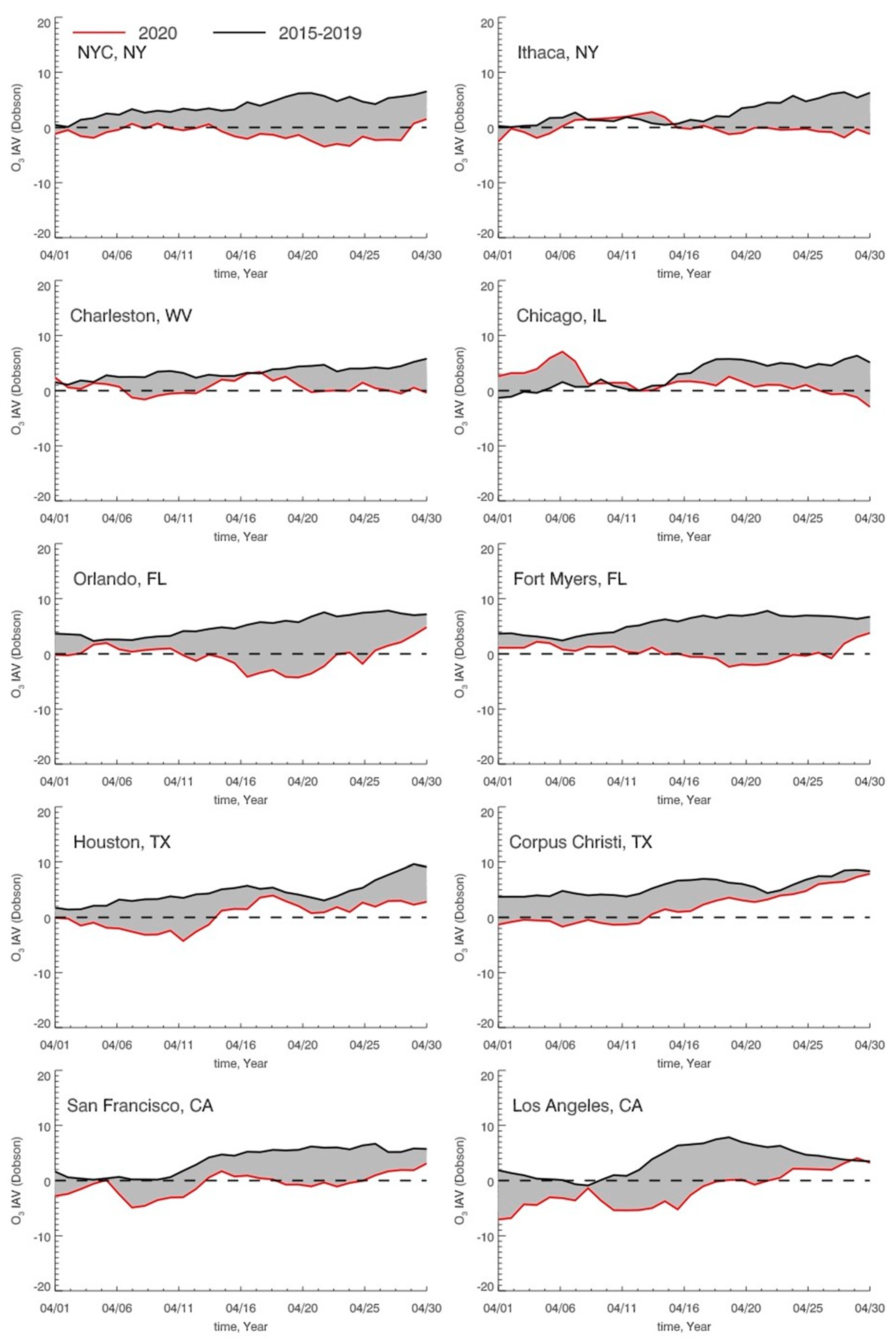
3.2.2. Interannual Variability and Significant Changes during the Lockdown
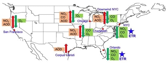
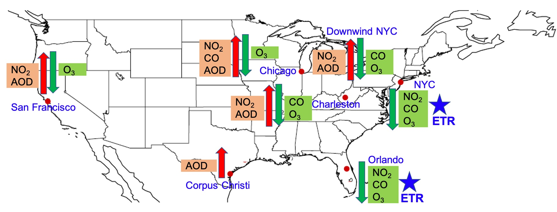
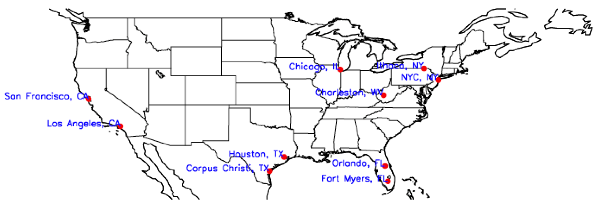
3.3. Regional Impacts
3.3.1. Northeast
3.3.2. Midwest
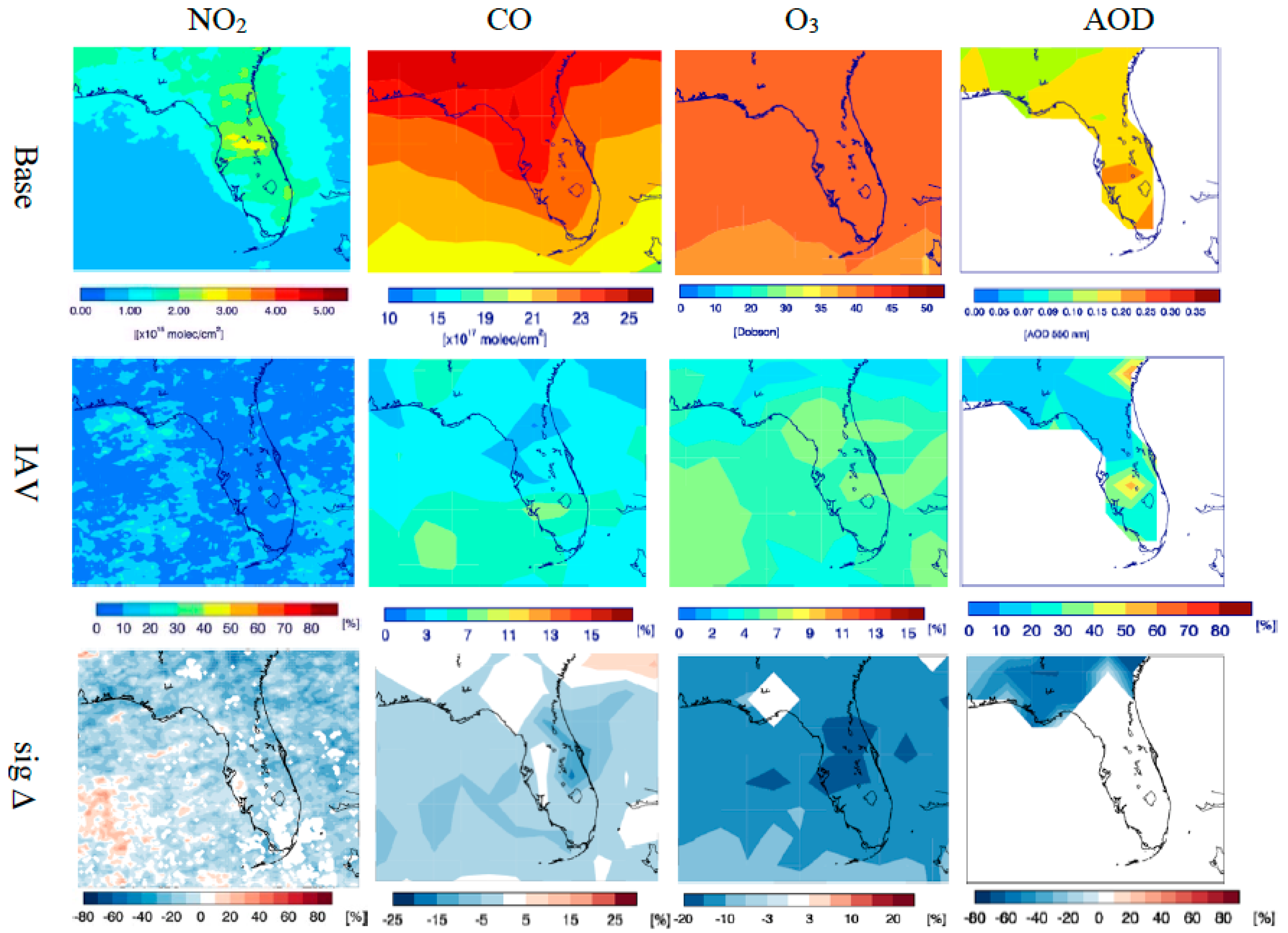
3.3.3. Southeast
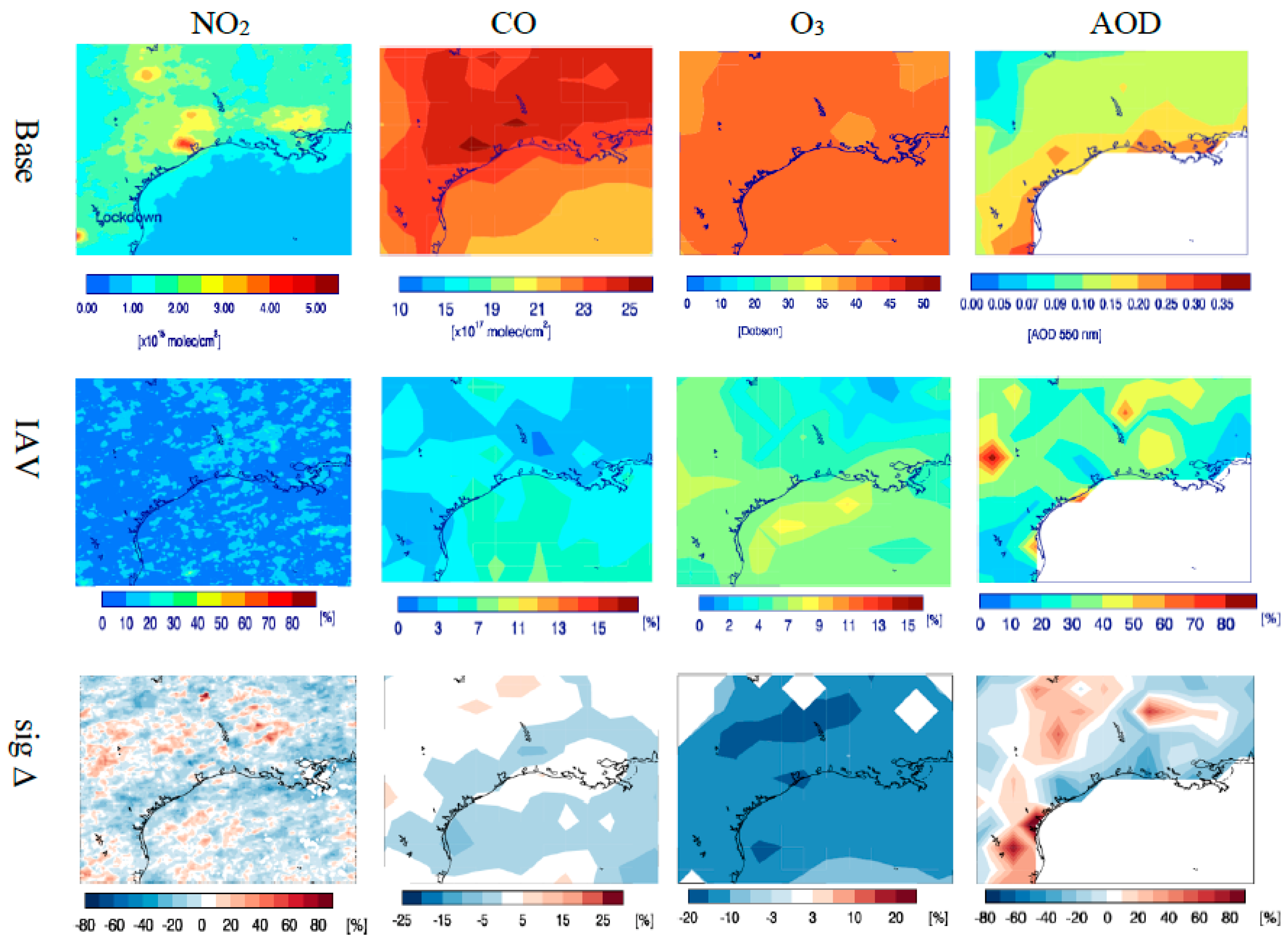
3.3.4. South
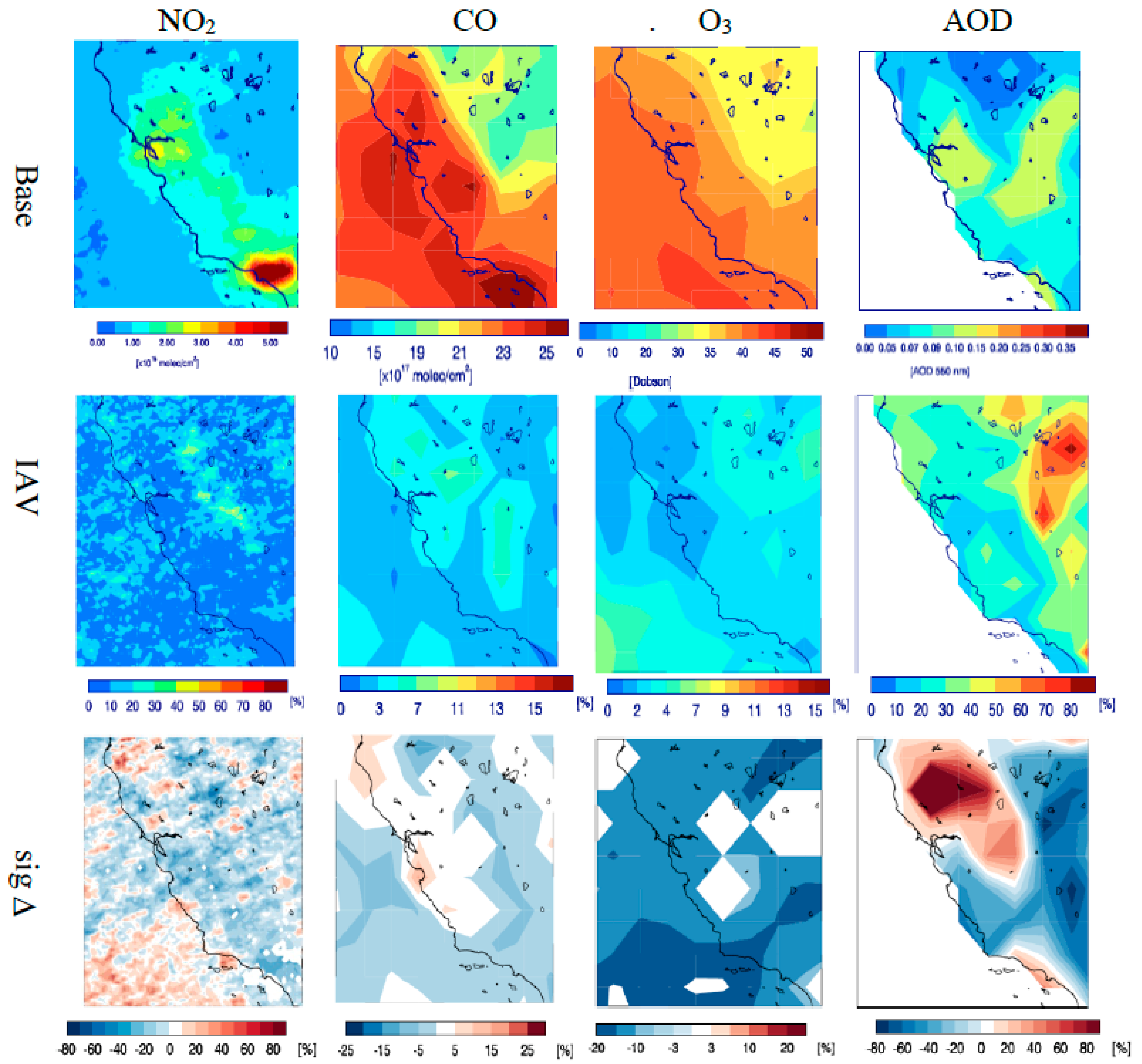
3.3.5. West Coast
4. Conclusions
Supplementary Materials
Author Contributions
Funding
Institutional Review Board Statement
Informed Consent Statement
Data Availability Statement
Conflicts of Interest
References
- WHO. The World Health Organization. Coronavirus Disease (COVID-19) Pandemic. Available online: https://www.who.int/emergencies/diseases/novel-coronavirus-2019 (accessed on 10 October 2020).
- CDC. Center for Disease Control and Prevention. Available online: https://COVID.cdc.gov/COVID-data-tracker/ (accessed on 12 October 2020).
- Hopkins, J. Coronavirus Resource Center. Available online: https://coronavirus.jhu.edu (accessed on 1 December 2020).
- De Haas, M.; Faber, R.; Hamersma, M. How COVID-19 and the Dutch “intelligent lockdown” change activities, work and travel behaviour: Evidence from longitudinal data in the Netherlands. Transp. Res. Interdiscip. Perspect. 2020, 6, 100150. [Google Scholar] [CrossRef]
- Beck, M.J.; Hensher, D.A. Insights into the impact of COVID-19 on household travel and activities in Australia—The early days under restrictions. Transp. Policy 2020, 96, 76–93. [Google Scholar] [CrossRef] [PubMed]
- Parr, S.; Wolshon, B.; Renne, J.; Murray-Tuite, P.; Kim, K. Traffic Impacts of the COVID-19 Pandemic: Statewide Analysis of Social Separation and Activity Restriction. Nat. Hazards Rev. 2020, 21. [Google Scholar] [CrossRef]
- Cartenì, A.; Di Francesco, L.; Martino, M. How mobility habits influenced the spread of the COVID-19 pandemic: Results from the Italian case study. Sci. Total Environ. 2020, 741, 140489. [Google Scholar] [CrossRef] [PubMed]
- Hadjidemetriou, G.M.; Sasidharan, M.; Kouyialis, G.; Parlikad, A.K. The impact of government measures and human mobility trend on COVID-19 related deaths in the UK. Transp. Res. Interdisc. Perspect. 2020, 6, 100167. [Google Scholar]
- Colvile, R.N.; Hutchinson, E.J.; Mindell, J.S.; Warren, R.F. The transport sector as a source of air pollution. Atmos. Environ. 2001, 35, 1537–1565. [Google Scholar] [CrossRef]
- O’Driscoll, R.; Stettler, M.E.J.; Molden, N.; Oxley, T.; ApSimon, H.M. Real world CO2 and NOx emissions from 149 euro 5 and 6 diesel, gasoline and hybrid passenger cars. Sci. Total Environ. 2018, 621, 282–290. [Google Scholar] [CrossRef]
- Vojtíšek-Lom, M.; Beranek, V.; Klír, V.; Jindra, P.; Pechout, M.; Voříšek, T. On-road and laboratory emissions of NO, NO2, NH3, N2O and CH4 from late-model EU light utility vehicles: Comparison of diesel and CNG. Sci. Total Environ. 2018, 616, 774–784. [Google Scholar] [CrossRef]
- Elshorbany, Y.F.; Kleffmann, J.; Kurtenbach, R.; Rubio, R.; Lissi, E.; Villena, G.; Rickard, A.R.; Pilling, M.J.; Wiesen, P. Summertime Photochemical Ozone Formation in Santiago de Chile. Atmos. Environ. 2009, 43, 6398–6420. [Google Scholar] [CrossRef]
- Liu, F.; Page, A.; Strode, S.A.; Yoshida, Y.; Choi, S.; Zheng, B.; Lamsal, L.N.; Li, C.; Krotkov, N.A.; Eskes, H.; et al. Abrupt decline in tropospheric nitrogen dioxide over China after the outbreak of COVID-19. Sci. Adv. 2020, 6, 28. [Google Scholar] [CrossRef]
- Venter, Z.S.; Aunan, K.; Chowdhury, S.; Lelieveld, J. COVID-19 lockdowns cause global air pollution declines. Natl. Acad. Sci. 2020, 117, 18984–18990. [Google Scholar] [CrossRef] [PubMed]
- Putaud, J.-P.; Pozzoli, L.; Pisoni, E.; Martins Dos Santos, S.; Lagler, F.; Lanzani, G.; Dal Santo, U.; Colette, A. Impacts of the COVID-19 lockdown on air pollution at regional and urban background sites in northern Italy. Atmos. Chem. Phys. Discuss. 2020. in review. [Google Scholar] [CrossRef]
- Pathakoti, M.; Muppalla, A.; Hazra, S.; Dangeti, M.; Shekhar, R.; Jella, S.; Mullapudi, S.S.; Andugulapati, P.; Vijayasundaram, U. An assessment of the impact of a nation-wide lockdown on air pollution—A remote sensing perspective over India. Atmos. Chem. Phys. Discuss. 2020. in review. [Google Scholar] [CrossRef]
- Chen, L.-W.A.; Chien, L.-C.; Li, Y.; Lin, G. Nonuniform impacts of COVID-19 lockdown on air quality over the United States. Sci. Total Environ. 2020, 745, 141105. [Google Scholar] [CrossRef]
- Zangari, S.; Hill, D.T.; Charette, A.T.; Mirowsky, J.E. Air quality changes in New York City during the COVID-19 pandemic. Sci. Total Environ. 2020, 742, 140496. [Google Scholar] [CrossRef]
- Huang, G.; Sun, K. Non-Negligible impacts of clean air regulations on the reduction of tropospheric NO2 over East China during the COVID-19 pandemic observed by OMI and TROPOMI. Sci. Total Environ. 2020, 745. [Google Scholar] [CrossRef]
- Bauwens, M.; Compernolle, S.; Stavrakou, T.; Müller, J.; Gent, J.; Eskes, H.; Levelt, P.F.; van der A, R.; Veefkind, J.P.; Vlietinck, J.; et al. Impact of Coronavirus Outbreak on NO2 Pollution Assessed Using TROPOMI and OMI Observations. Geophys. Res. Lett. 2020, 47. [Google Scholar] [CrossRef]
- Tobías, A.; Carnerero, C.; Reche, C.; Massagué, J.; Via, M.; Minguillón, M.C.; Alastuey, A.; Querol, X. Changes in air quality during the lockdown in Barcelona (Spain) one month into the SARS-CoV-2 epidemic. Sci. Total Environ. 2020, 726, 138540. [Google Scholar] [CrossRef]
- Zheng, H.; Kong, S.; Chen, N.; Yan, Y.; Liu, D.; Zhu, B.; Xu, K.; Cao, W.; Ding, Q.; Lan, B.; et al. Significant changes in the chemical compositions and sources of PM2.5 in Wuhan since the city lockdown as COVID-19. Sci. Total Environ. 2020, 739, 140000. [Google Scholar] [CrossRef]
- Ding, J.; van der A, R.J.; Eskes, H.; Mijling, B.; Stavrakou, T.; van Geffen, J.; Veefkind, P. NOx emissions reduction and rebound in China due to the COVID-19 crisis. Earth Space Sci. Open Arch. 2020, 47. [Google Scholar] [CrossRef]
- Cazorla, M.; Herrera, E.; Palomeque, E.; Saud, N. What the COVID-19 lockdown revealed about photochemistry and ozone production in Quito, Ecuador. Atmos. Pollut. Res. 2020, in press. [Google Scholar] [CrossRef] [PubMed]
- Huang, X.; Ding, A.; Gao, J.; Zheng, B.; Zhou, D.; Qi, X.; Tang, R.; Wang, J.; Ren, C.; Nie, W.; et al. Enhanced secondary pollution offset reduction of primary emissions during COVID-19 lockdown in China. Natl. Sci. Rev. 2020, 1–9, nwaa137. [Google Scholar] [CrossRef]
- Wang, P.; Chen, K.; Zhu, S.; Wang, P.; Zhang, H. Severe air pollution events not avoided by reduced anthropogenic activities during COVID-19 outbreak. Resour. Conserv. Recycl. 2020, 158, 104814. [Google Scholar] [CrossRef] [PubMed]
- El-Sayed, M.; Elshorbany, Y.; Koehler, K. On the impact of COVID-19 pandemic on air quality in FL. 2021; in preparation. [Google Scholar]
- Bekbulat, B.; Apte, J.S.; Millet, D.B.; Robinson, A.; Wells, K.C.; Marshall, J.D. PM2.5 and Ozone Air Pollution Levels Have Not Dropped Consistently Across the US Following Societal COVID Response. ChemRxiv 2020. [Google Scholar] [CrossRef]
- Federal Highway Administration (FHWA). Highway Performance Monitoring System (HPMS). Available online: https://www.fhwa.dot.gov/policyinformation/hpms/hpmsprimer.cfm (accessed on 13 July 2020).
- Shilling, F. Special Report (Update): Impact of COVID19 Mitigation on Numbers and Costs of California Traffic Crashes; Road Ecology Center: Davis, CA, USA, 2020; Available online: https://roadecology.ucdavis.edu/files/content/projects/COVID_CHIPs_Impacts_updated_415_1.pdf (accessed on 1 October 2020).
- Lamsal, L.N.; Krotkov, N.A.; Vasilkov, A.; Marchenko, S.; Qin, W.; Yang, E.-S.; Fasnacht, Z.; Joiner, J.; Choi, S.; Haffner, D.; et al. OMI/Aura Nitrogen Dioxide Standard Product with Improved Surface and Cloud Treatments. Atmos. Meas. Tech. Discuss. 2020. in review. [Google Scholar] [CrossRef]
- Barret, B.; DeMazière, M.; Mahieu, E. Ground-Based FTIP measurements of CO from Jungfraujoch: Characterisation and comparison with in situ surface and MOPITT data. Atmos. Chem. Phys. 2003, 3, 2217. [Google Scholar] [CrossRef]
- Buchholz, R.R.; Deeter, M.N.; Worden, H.M.; Gille, J.; Edwards, D.P.; Hannigan, J.W.; Jones, N.B.; Paton-Walsh, C.; Griffith, D.W.T.; Smale, D.; et al. Validation of MOPITT carbon monoxide using ground-based Fourier transform infrared spectrometer data from NDACC. Atmos. Meas. Tech. 2017, 10, 1927–1956. [Google Scholar] [CrossRef]
- Wei, J.; Li, Z.; Peng, Y.; Sun, L. MODIS Collection 6.1 aerosol optical depth products over land and ocean: Validation and comparison. Atmos. Environ. 2019, 201, 428–440. [Google Scholar] [CrossRef]
- Hsu, N.C.; Jeong, M.-J.; Bettenhausen, C.; Sayer, A.M.; Hansell, R.; Seftor, C.S.; Huang, J.; Tsay, S.-C. Enhanced Deep Blue Aerosol Retrieval Algorithm: The Second Generation. J. Geophys. Res. 2013, 118. [Google Scholar] [CrossRef]
- Sayer, A.M.; Hsu, N.C.; Lee, J.; Kim, W.V.; Dutcher, S.T. Validation, stability, and consistency of MODIS collection 6.1 and VIIRS version 1 Deep Blue aerosol data over land. J. Geophys. Res. Atmos. 2019, 124, 4658–4688. [Google Scholar] [CrossRef]
- Ziemke, J.R.; Chandra, S.; Duncan, B.N.; Froidevaux, L.; Bhartia, P.K.; Levelt, P.F.; Waters, J.W. Tropospheric ozone determined from Aura OMI and MLS: Evaluation of measurements and comparison with the Global Modeling Initiative’s Chemical Transport Model. J. Geophys. Res. 2006, 111, D19303. [Google Scholar] [CrossRef]
- McPeters, R.D.; Frith, S.M.; Kramarova, N.A.; Ziemke, J.R.; Labow, G.L. OMI total column ozone: Extending the long-term data record. Atmos. Meas. Tech. 2019, 8, 4845–4850. [Google Scholar] [CrossRef]
- Gelaro, R.; McCarty, W.; Suárez, M.J.; Todling, R.; Molod, A.; Takacs, L.; Randles, C.A.; Darmenov, A.; Bosilovich, M.G.; Reichle, R.; et al. The Modern-Era Retrospective Analysis for Research and Applications, Version 2 (MERRA-2). J. Clim. 2017, 30, 5419–5454. [Google Scholar] [CrossRef]
- Tropospheric Ozone Public Domain. Available online: https://gmao.gsfc.nasa.gov/reanalysis/MERRA-2 (accessed on 3 December 2020).
- Lee, H.; Garay, M.J.; Kalashnikova, O.V.; Yu, Y.; Gibson, P.B. How Long should the MISR Record Be when Evaluating Aerosol Optical Depth Climatology in Climate Models? Remote Sens. 2018, 10, 1326. [Google Scholar] [CrossRef]
- Shi, H.; Xiao, Z.; Ma, H.; Tian, X. Evaluation of MODIS and two reanalysis aerosol optical depth products over AERONET sites. Atmos. Res. 2019, 220, 75–80. [Google Scholar] [CrossRef]
- Devore, J. Probability and Statistics for Engineering and the Sciences, 8th ed.; California Polytechnic State University: San Luis Obispo, CA, USA, 2012; ISBN 13-978-0-538-73352-6. [Google Scholar]
- Huang, N.E.; Shen, Z.; Long, S.R.; Wu, M.C.; Shih, H.H.; Zheng, Q.; Yen, N.-C.; Chao, C. The Empirical Mode Decomposition and the Hilbert Spectrum for Nonlinear and Non-Stationary Time Series Analysis. Proc. R. Soc. Lond. 1998, 454, 903–995. [Google Scholar] [CrossRef]
- Wu, Z.; Norden, E.H.; Long, S.R.; Peng, C.K. On the trend, detrending, and variability of nonlinear and nonstationary time series. Proc. Natl. Acad. Sci. USA 2007, 104, 14889–14894. [Google Scholar] [CrossRef]
- Jiang, C.; Ryu, Y.; Fang, H.; Myneni, R.; Claverie, M.; Zhu, Z. Inconsistencies of interannual variability and trends in long-term satellite leaf area index products. Glob. Chang. Biol. 2017, 23, 4133–4146. [Google Scholar] [CrossRef]
- Jones, C.; Kammen, D.M. Spatial Distribution of U.S. Household Carbon Footprints Reveals Suburbanization Undermines Greenhouse Gas Benefits of Urban Population Density. Environ. Sci. Technol. 2014, 48, 895–902. [Google Scholar] [CrossRef]
- US Department of Transportation. Transportation GHG Emissions and Trends. Available online: https://www.transportation.gov/sustainability/climate/transportation-ghg-emissions-and-trends (accessed on 22 October 2020).
- Gately, C.; Hutyra, L.R.; Wing, I.S. DARTE Annual On-Road CO2 Emissions on a 1-km Grid, Conterminous USA, V2, 1980–2017; ORNL DAAC: Oak Ridge, TN, USA, 2019. [Google Scholar] [CrossRef]
- Elshorbany, Y.F.; Duncan, B.N.; Strode, S.A.; Wang, J.S.; Kouatchou, J. The description and validation of the computationally Efficient CH4–CO–OH (ECCOHv1.01) chemistry module for 3-D model applications. Geosci. Model Dev. 2016, 9, 799–822. [Google Scholar] [CrossRef]
- Hoesly, R.M.; Smith, S.J.; Feng, L.; Klimont, Z.; Janssens-Maenhout, G.; Pitkanen, T.; Seibert, J.J.; Vu, L.; Andres, R.J.; Bolt, R.M.; et al. Historical (1750–2014) anthropogenic emissions of reactive gases and aerosols from the Community Emission Data System (CEDS). Geosci. Model Dev. 2018, 11, 369–408. [Google Scholar] [CrossRef]
- Krotkov, N.A.; McLinden, C.A.; Li, C.; Lamsal, L.N.; Celarier, E.A.; Marchenko, S.V.; Swartz, W.H.; Bucsela, E.J.; Joiner, J.; Duncan, B.N.; et al. Aura OMI observations of regional SO2 and NO2 pollution changes from 2005 to 2015. Atmos. Chem. Phys. 2016, 16, 4605–4629. [Google Scholar] [CrossRef]
- Elshorbany, Y.F.; Crutzen, P.J.; Steil, B.; Pozzer, A.; Tost, H.; Lelieveld, J. Global and regional impacts of HONO on the chemical composition of clouds and aerosols. Atmos. Chem. Phys. 2014, 14, 1167–1184. [Google Scholar] [CrossRef]
- Simon, H.; Reff, A.; Wells, B.; Xing, J.; Frank, N. Ozone Trends Across the United States over a Period of Decreasing NOx and VOC Emissions. Environ. Sci. Technol. 2015, 49, 186–195. [Google Scholar] [CrossRef]
- Jaffe, D.A.; Cooper, O.R.; Fiore, A.M.; Henderson, B.H.; Tonnesen, G.S.; Russell, A.G.; Henze, D.K.; Langford, A.O.; Lin, M.; Moore, T. Scientific assessment of background ozone over the U.S.: Implications for air quality management. Elem. Sci. Anth. 2018, 6, 56. [Google Scholar] [CrossRef]
- Yang, Q.; Yuan, Q.; Yue, L.; Li, T.; Shen, H.; Zhang, L. The relationships between PM2.5 and aerosol optical depth (AOD) in mainland China: About and behind the spatio-temporal variations. Environ. Pollut. 2019, 248, 526–535. [Google Scholar] [CrossRef]
- Stirnberg, R.; Cermak, J.; Andersen, H. An Analysis of Factors Influencing the Relationship between Satellite-Derived AOD and Ground-Level PM10. Remote Sens. 2018, 10, 1353. [Google Scholar] [CrossRef]
- Berman, J.D.; Ebisu, K. Changes in U.S. air pollution during the COVID-19 pandemic. Sci. Total Environ. 2020, 739, 139864. [Google Scholar] [CrossRef]
- Roy, P. Atmospheric Smog Modeling, Using EOS Satellite ASTER Image Sensor, with Feature Extraction for Pattern Recognition Techniques and Its Correlation with In-Situ Ground Sensor Data. Ph.D. Thesis, Marshall University, Huntington, WV, USA, 2007. Available online: https://mds.marshall.edu/cgi/viewcontent.cgi?referer=https://www.google.com/&httpsredir=1&article=1817&context=etd (accessed on 27 October 2020).
- Lewis, C.W.; Macias, E.S. Composition of size-fractionated aerosol in Charleston, West Virginia. Atmos. Environ. 1979, 14, 185–194. [Google Scholar] [CrossRef]
- Kleinman, L.I.; Daum, P.H.; Lee, Y.-N.; Nunnermacker, L.J.; Springston, S.R.; Weinstein-Lloyd, J.; Rudolph, J. A comparative study of ozone production in 5 U.S. metropolitan areas. J. Geophys. Res. 2005, 110, D02301. [Google Scholar] [CrossRef]
- Shah, V.; Jaeglé, L.; Jimenez, J.L.; Schroder, J.C.; Campuzano-Jost, P.; Campos, T.L.; Reeves, J.M.; Stell, M.; Brown, S.S.; Lee, B.H.; et al. Widespread pollution from secondary sources of organic aerosols during winter in the Northeastern United States. Geophys. Res. Lett. 2019, 46, 2974–2983. [Google Scholar] [CrossRef]
- Schroder, J.C.; Campuzano-Jost, P.; Day, D.A.; Shah, V.; Larson, K.; Sommers, J.M.; Sullivan, A.P.; Campos, T.; Reeves, J.M.; Hills, A.; et al. Sources and secondary production of organic aerosols in the northeastern United States during WINTER. J. Geophys. Res. Atmos. 2018, 123, 7771–7796. [Google Scholar] [CrossRef]
- Li, K.; Liggio, J.; Han, C.; Liu, Q.; Moussa, S.G.; Lee, P.; Li, S.-M. Understanding the Impact of High-NOx Conditions on the Formation on Secondary Organic Aerosol in the Photooxidation of Oil Sand-Related Precursors. Environ. Sci. Technol. 2019, 53, 14420–14429. [Google Scholar] [CrossRef] [PubMed]
- Cohen, M.A.; Ryan, P.B.; Spengler, J.D.; Özkaynak, H.; Hayes, C. Source-Receptor study of volatile organic compounds and particulate matter in the Kanawha Valley, WV—I. Methods and descriptive statistics. Atmos. Environ. 1991, 25B, 79–93. [Google Scholar] [CrossRef]
- Lyons, W.A. The climatology and prediction of the Chicago Lake Breeze. J. Appl. Meteorol. 1972, 11, 1259–1270. [Google Scholar] [CrossRef]
- Fosco, T.; Schmeling, M. Aerosol ion concentration dependence on atmospheric conditions in Chicago. Atmos. Environ. 2006, 40, 6638–6649. [Google Scholar] [CrossRef]
- Xiang, S.; Hu, Z.; Zhai, W.; Wen, D.; Noll, K.E. Concentration of Ultrafine Particles near Roadways in an Urban Area in Chicago, Illinois. Aerosol. Air Qual. Res. 2018, 18, 895–903. [Google Scholar] [CrossRef]
- Tominack, S.A.; Coffey, K.Z.; Yoskowitz, D.; Sutton, G.; Wetz, M.S. An assessment of trends in the frequency and duration of Karenia brevis red tide blooms on the South Texas coast (western Gulf of Mexico). PLoS ONE 2020, 15, e0239309. [Google Scholar] [CrossRef]
- Cheng, Y.S.; Villareal, T.A.; Zhou, Y.; Gao, J.; Pierce, R.H.; Wetzel, D.; Naar, J.; Baden, D.G. Characterization of red tide aerosol on the Texas coast. Harmful Algae 2005, 4, 87–94. [Google Scholar] [CrossRef]
- Hu, C.; Muller-Karger, F.E.; Taylor, C.J.; Carder, K.L.; Kelble, C.; Johns, E.; Heil, C.A. Red tide detection and tracing using MODIS fluorescence data: A regional example in SW FL coastal waters. Remote Sens. Environ. 2005, 97, 311–321. [Google Scholar] [CrossRef]
- Faloona, I.C.; Chiao, S.; Eiserloh, A.J.; Alvarez, R.J.; Kirgis, G.; Langford, A.O.; Senff, C.J.; Caputi, D.; Hu, A.; Iraci, L.T.; et al. The California Baseline Ozone Transport Study (CABOTS). Bull. Am. Meteor. Soc. 2020, 101, E427–E445. [Google Scholar] [CrossRef]
- Zhao, K.; Bao, Y.; Huang, J.; Wu, Y.; Moshary, F.; Arend, M.; Wang, Y.; Lee, X. A high-resolution modeling study of a heat wave-driven ozone exceedance event in New York City and surrounding regions. Atmos. Environ. 2019, 199. [Google Scholar] [CrossRef]


| Parameter | Resolution | Instrument/Platform | Reference Period |
|---|---|---|---|
| NO2 | 0.1° | OMI/Aura | 2015–2019 |
| CO | 1° | MOPITT/TERRA | 2015–2019 |
| AOD | 1° | MODIS DB land/TERRA | 2010–2019 |
| Ozone | 1° | OMPS/MERRA-2 | 2015–2019 |
Publisher’s Note: MDPI stays neutral with regard to jurisdictional claims in published maps and institutional affiliations. |
© 2021 by the authors. Licensee MDPI, Basel, Switzerland. This article is an open access article distributed under the terms and conditions of the Creative Commons Attribution (CC BY) license (http://creativecommons.org/licenses/by/4.0/).
Share and Cite
Elshorbany, Y.F.; Kapper, H.C.; Ziemke, J.R.; Parr, S.A. The Status of Air Quality in the United States During the COVID-19 Pandemic: A Remote Sensing Perspective. Remote Sens. 2021, 13, 369. https://doi.org/10.3390/rs13030369
Elshorbany YF, Kapper HC, Ziemke JR, Parr SA. The Status of Air Quality in the United States During the COVID-19 Pandemic: A Remote Sensing Perspective. Remote Sensing. 2021; 13(3):369. https://doi.org/10.3390/rs13030369
Chicago/Turabian StyleElshorbany, Yasin F., Hannah C. Kapper, Jerald R. Ziemke, and Scott A. Parr. 2021. "The Status of Air Quality in the United States During the COVID-19 Pandemic: A Remote Sensing Perspective" Remote Sensing 13, no. 3: 369. https://doi.org/10.3390/rs13030369
APA StyleElshorbany, Y. F., Kapper, H. C., Ziemke, J. R., & Parr, S. A. (2021). The Status of Air Quality in the United States During the COVID-19 Pandemic: A Remote Sensing Perspective. Remote Sensing, 13(3), 369. https://doi.org/10.3390/rs13030369