Abstract
Following the continuous and stable regional service of BDS2, the BDS3 officially announced its global service in July 2020. To fully take advantage of the new multi-frequency BDS3 signals in ionosphere sensing and positioning, it is essential to understand the characteristics of the differential code bias (DCB) of new BDS3 signals and BDS performance in global ionospheric maps (GIMs) estimation. This article presents an evaluation of the characteristics of 13 types of BDS DCBs and the accuracy of BDS-based GIM based on the data provided by the International GNSS Service (IGS) and International GNSS Monitoring and Assessment System (iGMAS) for the first time. The GIMs and DCBs are estimated by the APM (Innovation Academy for Precision Measurement Science and Technology) method in a time efficient manner, which can be divided into two main steps. The first step is to produce GIMs based on BDS observations at the B1I, B2I and B3I signals, and the second step is to estimate DCBs among the other frequency bands by removing the ionospheric delay using the precomputed GIMs. Good agreement is found between the APM-based satellite DCB estimates and those from the Chinese Academy of Sciences (CAS) and the German Aerospace Center (DLR) at levels of 0.26 ns and 0.18 ns, respectively. The results, spanning one month, show that the stability of BDS DCB estimates among different frequency bands are related to the contributed observations, and the receiver DCB estimates represent larger STD values than the satellite DCB estimates. The differences in receiver DCB estimates between BDS2 and BDS3 are found to be related to the types of receivers and antennas and firmware version, and the bias of the JAVAD receivers reaches 1.03 ns. The results also indicate that the difference in the single-frequency standpoint positioning (SPP) accuracy using GPS-based and BDS-based GIMs for ionospheric delay corrections is less than 0.03 m in both the horizontal and vertical directions.
1. Introduction
As the third global navigation satellite system (GNSS) following the great successes of the GPS and GLONASS systems, the BeiDou navigation satellite system (BDS) has evolved from a regional navigation satellite system (BDS2) to the third generation of the navigation satellite system (BDS3) with global coverage [1]. The BDS2 has provided services mainly in the Asia-Pacific area since 27 December 2012.The completion of BDS3 was officially announced on 31 July 2020, after which BDS3 started to provide services at its full operational capability, including positioning, timing and short message communications [1]. As shown in Table 1, BDS2 currently consists of three medium earth orbit (MEO) satellites, five geostationary earth orbit (GEO) satellites and seven inclined geosynchronous orbit (IGSO) satellites. As shown in Table 2, by June 2020, the BDS3 system consisted of three IGSO satellites, two GEO satellites and 24 MEO satellites [2].

Table 1.
Status of healthy BDS2 satellites (as of June 2020).
Table 2.
Status of healthy BDS3 satellites (as of June 2020).
The BDS2 satellites transmit triple frequency signals centered at B1I, B2I and B3I. In BDS3, signals with different modulation techniques and chip rates at a total of six frequencies are transmitted, including the new B1C, B2a, B2b and B2ab signals and the original B1I and B3I signals [3]. To track and analyze multifrequency observations and broadcast navigation-related messages from multi-GNSSs, several publicly accessible global networks of monitoring stations have been set up by various institutions, including the international GNSS service (IGS) multi-GNSS experiment (MGEX) network [4], the Chinese international GNSS monitoring and assessment system (iGMAS) tracking network [5] and the Australian continuously operating reference stations (AUSCORS) [6]. By June 2020, more than 240 receivers worldwide that support BDS2 signal tracking and 160 receivers that support BDS3 signal tracking were accessible. Multifrequency BDS signals tracked by globally distributed monitoring stations offer a basis for the independent monitoring of the global ionospheric total electron content (TEC).
Ionospheric effects need to be eliminated in GNSS data processing for precise navigation and positioning applications [7]. On the other hand, the computation of reliable global ionospheric maps (GIMs) of vertical TEC (VTEC) based on GNSS data provides valuable information in both science and technology fields, such as space weather monitoring and user navigation improvement [8,9]. Thus, the performance of the GIMs computed based on the GNSS data can be regarded as an important index that scales the whole performance of one specific navigation system. With the aim of continually monitoring the ionosphere, GIMs developed by different techniques have been routinely provided by the IGS since 1998 [8]. Although there are currently seven IGS-related ionospheric associate analysis centers (IAACs), the GIMs provided by these IAACs are almost exclusively produced using only GPS/GLONASS data [10]. In addition, although ionospheric modeling based on BDS data has been analyzed in previous studies [11,12], most of these studies used data combinations from BDS and other GNSS systems. That is, due to the limited number of BDS satellites and the uneven distribution of stations available to track BDS3 signals before the completion of the establishment of BDS3, BDS data have not been applied in computations of IGS-related GIM products, and the issue of the performances of GIMs calculated using only BDS observations has not yet been reported.
Considering the effects of differential code bias (DCB) on ionospheric delay modeling and satellite clock correction, satellite and receiver DCBs are thought to be important parameters in the pseudorange-based positioning, navigation and timing (PNT) of GNSS-related and ionospheric research [13,14,15]. For the proper processing of linear combinations of code observations on multiple frequencies, two independent timing group delay (TGD) parameters, which are defined as the satellite DCBs between the antenna phase center of the B3I to B1I and B2I frequencies, namely TGD1 and TGD2, have been broadcast in navigation-related messages of the BDS [16,17,18,19]. In addition, two types of daily multi-GNSS DCB products have been routinely provided by the German Aerospace Center (DLR) and the Chinese Academy of Sciences (CAS) at the IGS CDDIS website [20]. The DLR-based DCBs are calculated by introducing an a priori ionospheric TEC [21], and the CAS-based DCBs are computed using combined estimations of DCBs and ionospheric parameters [22].
Due to the dispersive nature of ionospheric refractivity, the ionospheric observables are well known to be obtained from the geometry-free linear combination of dual-frequency GNSS measurements [23]. Thus, the accuracy of ionospheric TEC estimation can be improved by selecting two different frequencies with high-quality signals, and in this process, DCBs between different frequencies need to be precisely calibrated. To make full use of the new multifrequency BDS3 signals for positioning and ionospheric research, there is a strong need for precise handling of the BDS3 DCBs that are associated with the newly emerging frequencies. Although the estimation of BDS3 DCBs has been included in a few previous studies [5,24,25,26,27], further research should be performed, as existing studies have mainly focused on experimental satellites and few BDS3 satellites and a limited number of stations were applied. On one hand, existing studies related to the estimation and analysis of BDS DCBs mainly concentrated on C2I-C7I and C2I-C6I DCBs. The characteristics of the DCBs related to the new BDS3 signals have not yet been systematically studied. On the other hand, proper knowledge of whether there are intersystem biases between BDS3 and BDS2 receiver DCBs is of interest for users who need to jointly process BDS2 and BD3 data [25]. However, different conclusions have been drawn from the existing studies. Li et al. [5] found that an obvious systematic bias existed in the receiver DCB differences between BDS3 and BDS2 when different networks were processed together. Wang et al. [24] found no evident systematic bias between BDS2 and BDS2+BDS3 receiver DCBs.
The main objective of this study is to present a comprehensive evaluation of the characteristics of satellite and receiver DCBs for the new BDS3 signals and the performance of the BDS in modeling global ionospheric TEC. To this end, we carried out experiments and analyses based on BDS2 and BDS3 multifrequency observations collected at 246 IGMAS and MGEX sites during two selected periods in 2020. This paper proceeds as follows. First, the estimation method, which is named APM (Innovation Academy for Precision Measurement Science and Technology), and was used to determine the GIMs and DCBs in the BDS satellites and receivers, is introduced in detail. Then, the characteristics of 13 types of BDS2 and BDS3 DCBs, which have been defined as DCB between the C1X, C1P, C1B, C1A, C5I, C5X, C5Q, C5P, C6I, C7I, C7Z, C7A and C8X signals with respect to the C2I signal, are analyzed in detail. Finally, the performance of the GIMs is validated and evaluated in terms of comparisons with IGS-related final GIMs and standard point positioning (SPP).
2. Methodology
The APM algorithm used to estimate the BDS-based GIMs and the satellite and receiver DCBs between different frequencies in a time-efficient manner includes three main processing steps. First, the ionospheric observables are extracted from the original BDS pseudorange and carrier-phase observations based on the pseudorange-leveled carrier-phase approach [28,29]. Second, the GIMs are calculated by establishing a global ionospheric VTEC model. Third, the satellite and receiver DCBs between different frequency bands, including those of the new BDS3 signals, are calculated using the GIMs computed in the second step.
2.1. Extraction of Ionospheric Observables
Ignoring the effects of multiple paths and noise, the code and carrier-phase measurements in units of length can be expressed as follows [30]
where and are the code and carrier-phase measurements associated with receiver , satellite , carrier frequency band and epoch , respectively; denotes the combination of all frequency-independent terms, including the geometric distance from the satellite to the receiver , receiver clock errors , satellite clock offset and tropospheric delay ; is the slant ionospheric delay on the first frequency; is the frequency-dependent factor, where denotes the frequency of the carrier-phase; and are the receiver and satellite code hardware delays, respectively; and is the real-value ambiguity.
Based on Equation (1), the geometry-free code and carrier-phase observation equation can be constructed as follows [31]
where and denote the geometry-free code and carrier-phase observables between frequency bands and , respectively; and are the receiver and satellite DCBs, respectively, which are assumed to be constant over periods of 24 h; and denotes the geometry-free carrier-phase ambiguity.
As Equation (2) indicates, the non-dispersive effects have been removed and the ionospheric delay parameter changes between epochs, while the remaining parameters are assumed to be constant over time. Thus, the so-called leveling constant, which amounts to the sum of the satellite and receiver DCBs and the ambiguities, can be determined by averaging and for a continuous arc that consists of a total of t epochs, as follows
where is the operator that computes the average of the variables over epochs ().
By combining Equations (2) and (3), the ionospheric observable can be expressed as follows:
As such, ionospheric observables, which are linear combinations of the original slant ionospheric delay and the satellite and receiver DCBs, are extracted.
2.2. Establishment of a Thin-Layer Global Ionosphere Model
As expressed in Equation (4), the estimable ionospheric observables are coupled with DCBs. To obtain clean slant ionospheric delays, one interrelated task is to separate the satellite and receiver DCBs from the ionospheric observables. It has been demonstrated that the spherical harmonic function model can efficiently model spatial and temporal variability in global ionospheric TEC [8]. In this study, the VTEC is represented by a maximum degree and order equal to 15 spherical harmonic expansions with a 2-h resolution based on the so-called single-layer model [10], which reads as follows
where is the ionospheric VTEC at the ionospheric intersecting pierce point (IPP); and are the latitude and longitude of the IPP in the sun-fixed geomagnetism coordinate system; is the classical unnormalized Legendre function; is the normalization function; is the Kronecker delta; and and are the unknown spherical harmonic coefficients to be estimated.
With the reparameterized ionospheric delay replacing in Equation (4), we can rewrite the ionospheric observables as follows
where is the shell mapping function used to convert the slant TEC (STEC) along a given ray path to the VTEC, with , and being the satellite elevation angle, mean radius of Earth and altitude of the ionospheric thin-layer shell (450 km), respectively, and being the weight of the ionospheric observable, which is dependent on the elevation angle of the satellite.
In the parameter estimation process, piece-wise linear functions are used to guarantee the continuity of the TEC model between two neighboring sessions. Based on Equation (6), the spherical harmonic coefficients can be solved for based on least-squares adjustment, and can be further used to compute the VTEC values for the GIMs at the designated latitudes and longitudes. To improve the computational efficiency, only the ionospheric observables extracted based on the B1I, B2I and B3I signals are selected to estimate the spherical harmonic coefficients. An elevation cutoff angle of 15° is used to mitigate the impacts of multipath and mapping function errors at low elevations.
2.3. Estimation of BDS DCBs between the Different Frequency Bands
By correcting the ionospheric delay based on the GIM calculated with Equation (5), the satellite and receiver DCBs between different frequency bands can be estimated using the following equation
where in the second term is the VTEC at the IPP location calculated based on a bilinear interpolation in space and time on previously generated GIM. To eliminate the rank deficiency occurring between the satellite and receiver DCBs, the zero-mean constraint condition assuming that the sum of satellite DCBs of all satellites is equal to zero has been imposed in this study.
3. Results
In this chapter, we first describe the experimental datasets followed by the validation of the proposed APM method. Thereafter, analyses of the characteristics of satellite and receiver DCBs of the new BDS3 signals are conducted. Then, the performance of the GIMs estimated with only BDS data is analyzed.
3.1. Experimental Data
For our analysis, we selected two observation periods in 2020. The first period, covering six months, from day of year (DOY) 061 to 244, is used for validation of the APM method in terms of the accuracy of the APM-based satellite DCB estimates. The second period, covering 1 month, from DOY 214 to 244, is used for the analysis of DCBs for the BDS3 new signals and the BDS-based GIMs.
As shown in Figure 1, 246 globally distributed stations from the IGMAS and MGEX tracking networks were selected to perform the evaluation and analysis. The data sampling rate was chosen as 30 s. Table 3 summarizes the basic information of the tracking stations whose receiver types stayed unchanged during the period of DOY 214–244, 2020. The receiver hardware device information for stations whose receiver type or antenna type changed during the test period is listed in Table 4. Information on the BDS signals, including the signal frequencies, observation type and number of accessible stations, is listed in Table 5. Different colors used to denote stations in Figure 1 correspond to different receiver types in the first column, “Receiver type index”, in Table 5. As shown in Table 5, more than 180 receivers can track triple-frequency legacy BDS signals. The C7I signal can be tracked by the majority of receivers except the CETC-54-GMR, BD070 and GNSS_GGR receivers. Considering that the C2I signal can be tracked by all receivers, all DCBs estimated in this study are formed with respect to the C2I signal.
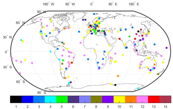
Figure 1.
Overview of the experimental multi-GNSS experiment (MGEX) and International GNSS Monitoring and Assessment System (iGMAS) stations. Different colors denote receivers from different manufacturers corresponding to the first column in Table 3.
Table 3.
Receiver and observation types based on RINEX observation codes.
Table 4.
Information on receiver types and antenna types used for the METG, SPT0 and YAR2 stations.
Table 5.
BDS signals and their corresponding frequencies and code observations.
As shown in Figure 2, 48 globally distributed MGEX stations were also selected to investigate the performance of the BDS-based GIM in the position domain. The station coordinates derived from the final IGS solutions were used as a reference to calculate the position errors.
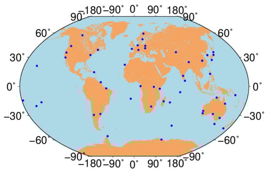
Figure 2.
Distributions of the selected sites.
3.2. Validation of the APM Method for BDS Satellite DCB Estimation
To test the effectiveness of the APM method, the overall performance of the APM-based BDS DCB estimates was first validated, by comparison with daily DCBs provided by DLR, CAS and TGD parameters collected from the BDS navigation message. The stability, expressed as the standard deviation (STD) of satellite DCB estimates and the consistency among different DCB solutions for the period from DOY 061 to 244, 2020 were employed as the two performance indicators.
Since the two TGD parameters (TGD1 and TGD2) can be interpreted as C2I-C6I and C7I-C6I DCBs, the C2I-C7I DCB is, in theory, equal to the TGD1-TGD2 parameter. Considering that the TGD1 parameter for BDS2 and BDS3 might refer to the respective reference datum [19], the BDS2 and BDS3 DCBs obtained from different solutions were first normalized by a zero-mean constraint across the respective full sets of the BDS2 or BDS3 satellites before comparison. Additionally, because the DCBs obtained from different solutions may be calculated based on different BDS satellites, this section presents only the results for the common satellites. For example, since the DCBs for BDS3 GEO satellites (PRN C59 and C60) are not provided by the CAS and the DCBs for the PRN C60 satellite are not provided by the DLR, the statistical results do not cover these two satellites.
To understand the stability of APM-based BDS satellite DCB estimates, the time series of the weekly STDs of the C2I-C6I and C2I-C7I DCB estimates during the test period are first calculated. As shown in Figure 3, abnormal variations occurred in the BDS DCB estimates for the PRN C01 and C28 satellites, indicating that the satellite DCBs are not always stable enough. The abnormal weekly mean DCB estimates for the PRN C01 satellite during the periods from DOY 084 to 097 can be attributed to the decreased DCB values of satellite C01 on DOY 091. Obvious jumps in the weekly mean DCB time series shown at the bottom of Figure 3 can be attributed to the DCB variation on DOY 135 for the PRN C28 satellite. Apart from the two obvious jumps in the weekly mean DCB time series shown in Figure 3, DCB estimates for the two satellites appear to be rather stable. The weekly STD values for satellites except PRN C01 and C28 are plotted in Figure 4. The maximum values of the STDs of the DCB estimates obtained from APM, DLR and CAS are 0.17, 0.15 and 0.23 ns, which shows the consistency of the stability of DCB estimates from the APM and other solutions. The mean STDs for the three DCB products over the test period are all less than 0.1 ns, which shows good repeatability of the BDS satellite DCB estimates.
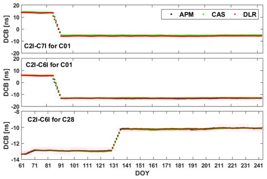
Figure 3.
Time series of weekly mean differential code biases (DCB) of the selected satellites during the period of day of year (DOY) 061–244 in 2020.
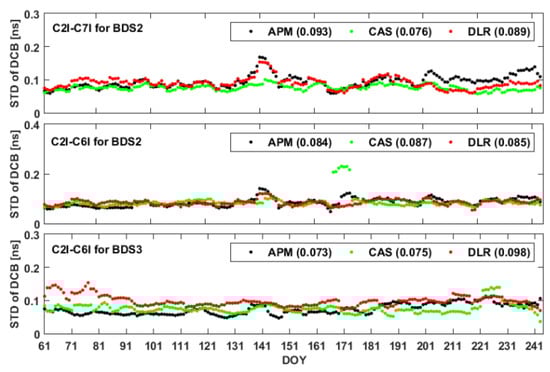
Figure 4.
Weekly STDs of the C2I-C6I and C2I-C7I DCB estimates during the period of DOY 061–244 in 2020.
Time series of the daily root mean square (RMS) values of the differences among different satellite DCB solutions during the test period are shown in Figure 5. The averaged RMS values are summarized in Table 6. The statistics show that the TGD-based DCBs represent the largest differences with respect to the other solutions. The averaged RMS values of the differences between the APM-based DCB estimates and the DLR and CAS products are less than 0.23 and 0.32 ns, respectively, showing the encouraging consistency of these three DCB estimation methods. Due to the similar DCB estimation strategy, the APM- and DLR-based DCBs have better agreement for both the BDS2 and BDS3 constellations than do the other DCB products. Table 6 shows the DCB estimates obtained from different solutions using BDS2 satellites show better consistency than those using BDS3 satellites. This finding is consistent with the study of Wang et al. [19], in which this phenomenon was attributed to the poor B1I-B3I dual-frequency coverage of the BDS3 satellites.
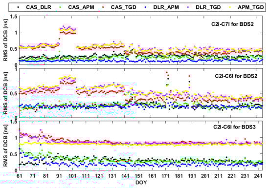
Figure 5.
Root mean square (RMS) time series of the differences in BDS-based C2I-C6I and C2I-C7I DCB estimates between different solutions during the period of DOY 061–244 in 2020.
Table 6.
Statistics of the mean RMSs of the differences between the different satellite-based DCB solutions during the period of DOY 061–244 in 2020, expressed in nanoseconds.
As shown in Figure 5, the differences between the TGD-based DCBs and the other DCB solutions decreased after DOY 141, 2020, suggesting that an improved strategy was used in the generation of broadcasted TGDs in BDS-based ground control segments. In addition, the RMS values of the differences of BDS2 DCBs between the TGD-based and other solutions have an obvious jump during the period of DOY 091–103 in 2020. To find the reason for the larger RMS for TGD-based DCBs, Figure 6 presents the RMS for each BDS2 satellites. From Figure 6, it may be concluded that the observed abnormal daily RMS values were largely driven by abnormal variations that occur in the RMS values for the PRN C01 satellite.
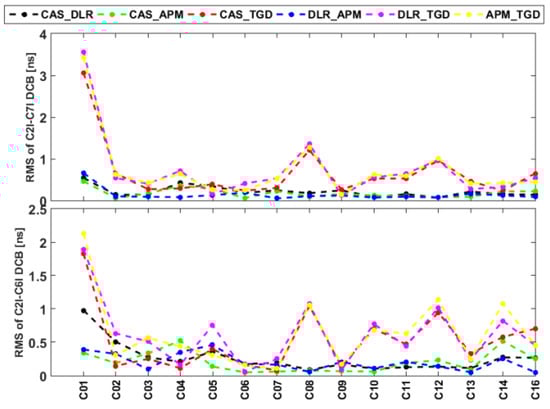
Figure 6.
RMS time series of the differences in BDS-based C2I-C6I and C2I-C7I DCB estimates between different solutions during the period of DOY 091–103 in 2020.
The mean differences observed among the BDS-based DCBs of individual satellites during the period of DOY 061-244 in 2020 are illustrated in Figure 7, and the RMS values of the differences among varying DCB estimates for different orbit types are summarized in Table 7. As seen from the statistics, the BDS2-based DCB differences among the different products of the IGSO satellites are smaller than those of the GEO and MEO satellites; however, this conclusion is not suitable for BDS3-based DCBs.
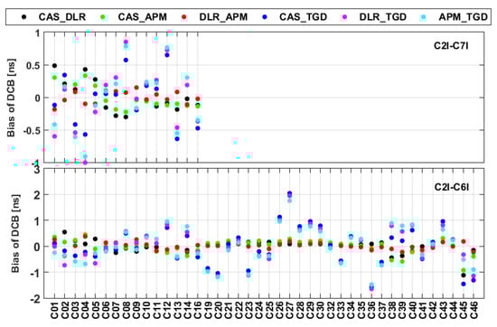
Figure 7.
The average differences among the different DCB solutions during the period of DOY 061–244 in 2020.
Table 7.
The average RMSs of the differences among the different DCB solutions during the period of DOY 061-244 in 2020 (unit: ns).
3.3. BDS Satellite-Based DCBs among Different Frequency Bands
The consistency between the APM-based BDS satellite DCB estimates and daily DCBs estimated by DLR and CAS has been validated in Section 3.2. To better understand the characteristics of the BDS3 satellite DCBs, mean values of the DCBs among the six different frequency bands covering all operational BDS3 satellites over a period of one month are shown in Figure 8. A close match of BDS3 DCBs between the same two frequency band signals can be noted from this figure. The DCBs between the B1I and B1C signals are confined to a range of ±5 ns, while the DCB values between B1I and other signals of the BDS3 satellites, with the exception of the PRN C33 satellite, are confined to a range of −31 to 55 ns.
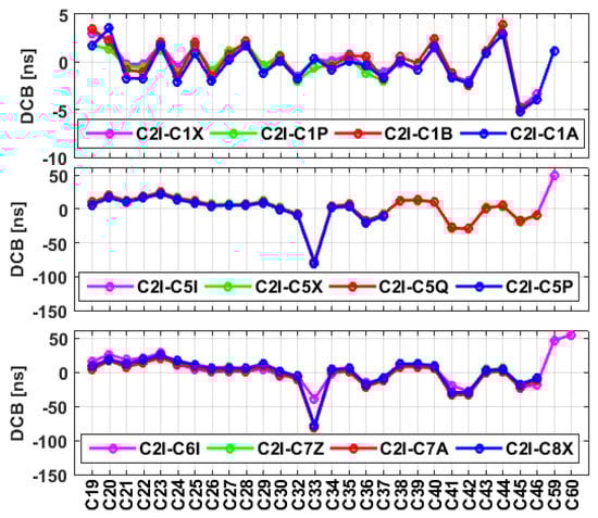
Figure 8.
Mean values of BDS3-based DCBs during the period of DOY 214–244 in 2020.
For evaluation of the stability of the BDS3 satellite-based DCBs, Figure 9 shows the monthly STDs of the BDS3 satellite-based DCB estimates of the signals among the different frequency bands. As shown in the figure, other than the C2I-C1A, C2I-C5Q, C2I-C5I and C2I-C7A DCB estimates, which exhibit large STDs, the STDs of the DCB estimates of the signal combinations are less than 0.2 ns. Similar to Figure 8 and Figure 9, the mean values and STDs of the DCB estimates of each BDS2 satellite are shown in Figure 10. The BDS2 satellite-based DCB estimates are confined to a range of ±20 ns. The monthly STDs of the BDS2 DCB estimates are mainly within 0.2 ns, showing better stability than those of the BDS3 satellites. In addition, because the signal quality of B3I is better than that of B2I [27], the stability of the C2I-C6I DCB estimates outperforms that of the C2I-C7I DCB estimates.
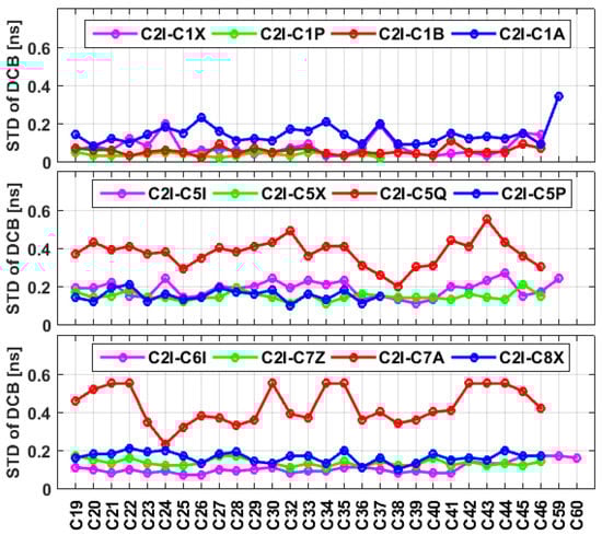
Figure 9.
Monthly stability of the BDS3-based DCB estimates during the period of DOY 214–244 in 2020.
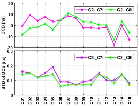
Figure 10.
Mean values and monthly stability of the BDS2-based DCB estimates for August 2020.
As seen from the statistics on the STDs of the DCB estimates of BDS2 and BDS3 shown in Figure 9 and Figure 10, the IGSO satellites show better stability than the GEO and MEO satellites. This phenomenon has been attributed to the longer observation arcs and wider geographic coverage of IGSO satellites than those of other satellites, as outlined in previous studies [32]. To better understand the impact of the contributed observables on the stability of BDS-based DCB estimates, taking the C2I-C6I DCB as an example, the numbers of tracking stations and contributed observations for each BDS satellite are shown in Figure 11. We can see that the number of stations available for the computation of daily GEO satellites is less than that of IGSO satellites. In addition, the number of contributing stations for the DCB estimation of satellites launched after 2019 is usually fewer than 50, and this can be regarded as one reason for the degraded stability of these newly launched satellites, compared to the remaining satellites. Although the B2ab signal has the best pseudorange measurement accuracy and the strongest anti-multipath ability among the different BDS3 signals [3], as shown in Figure 12, the STDs of the C2I-C8X DCBs are still larger than those of the C2I-C6I and C2I-C7Z DCBs. It may be concluded that the contributed number of observables has a larger impact on the stability of DCB estimates than the signal quality.
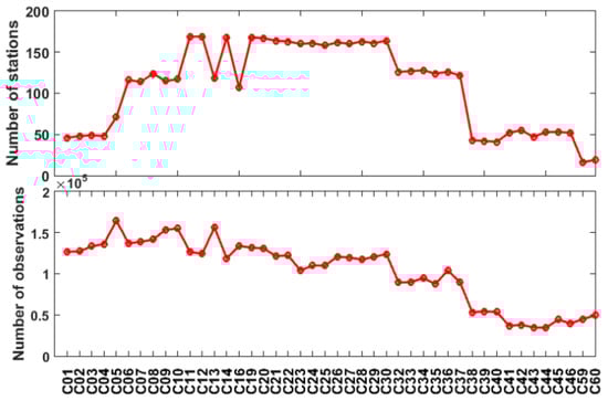
Figure 11.
Numbers of tracking stations and contributed observations for each BDS satellite in the C2I-C6I DCB estimation on DOY 214, 2020.
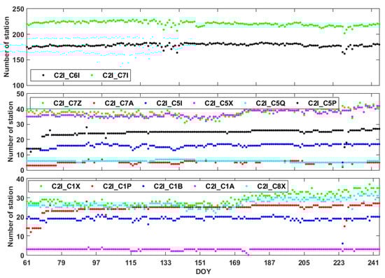
Figure 12.
Time series of the daily number of stations used to calculate the DCB solutions.
3.4. BDS Receiver-Based DCBs among Different Frequency Bands
To check whether systematic bias existed in the receiver DCBs between BDS3 and BDS2, we designed two sets of experiments with all accessible stations from the MGEX and IGMAS networks. In the first set of experiments, both BDS2 and BDS3 satellites are used to solve for the receiver DCBs. In the second set of experiments, only BDS2 satellites are used. Since differences exist in the numbers of contributing satellites, the zero-mean condition is also different between the two solutions. Considering that the zero-mean condition imposed on all available satellites is used in the two different solutions, to unify the BDS2+BDS3-based and BDS2-based DCB solutions, the DCB estimates are only normalized by a zero-mean condition for the commonly used BDS2 satellites.
Figure 13 shows the mean differences and STDs of the receiver C2I-C6I DCB estimates between BDS2-only and BDS2+BDS3 solutions during the period of DOY 214–244, 2020. There is no change in the receiver hardware device during the test period for receivers shown in this figure. The statistics shown in Table 8 reveal that the differences in receiver DCBs between the two different solutions have a strong dependence on the receiver type. This conclusion is in accordance with the study of Wang et al. [24]. Except for the SEPT and TRIMBLE receivers, the differences in receiver DCBs between the two different solutions are almost all positive. The BDS2 and BDS3 receiver DCB differences for SEPT receivers are all negative, while those for TRIMBLE receivers fluctuate around an average value at the level of 0.07 ns. The mean bias and STD of the estimated DCB differences between the BDS2-only and BDS2+BDS3 solutions for all receiver types are 0.16 ns and 0.12 ns, respectively.
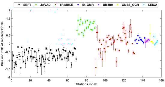
Figure 13.
Mean differences and STDs of receiver C2I-C6I DCB estimates between BDS2+BDS3 and BDS2-only solutions. The receivers are sorted by receiver type.
Table 8.
Consistency of receiver DCBs between BDS2-only and BDS2+BDS3 solutions during the test period (unit: ns).
To further analyze the impact of the antenna type and firmware version on the bias between the BDS2 and BDS3 receiver DCB estimates, taking the receiver type of TRIMBLE NETR9 as an example, Figure 14 shows the mean differences and STDs of the receiver DCB estimates between BDS2-only and BDS2+BDS3 solutions for the selected stations in three groups equipped with the same types of receivers and antennas and firmware version configuration. Table 9 shows the information of the three groups of stations and the corresponding statistical results. There are obvious significant differences in the bias results between receivers from different manufacturers. In addition, the mean differences of the receiver DCB estimates between BDS2-only and BDS2+BDS3 solutions for receivers in the second and third group are all positive values, and those of the first group are almost all negative values. It may be concluded that the differences in receiver DCB estimates between BDS2 and BDS3 are related to firmware version and types of receivers and antennas, and the firmware version has a larger impact on the bias between the BDS2 and BDS3 receiver DCBs than that of the antenna type.
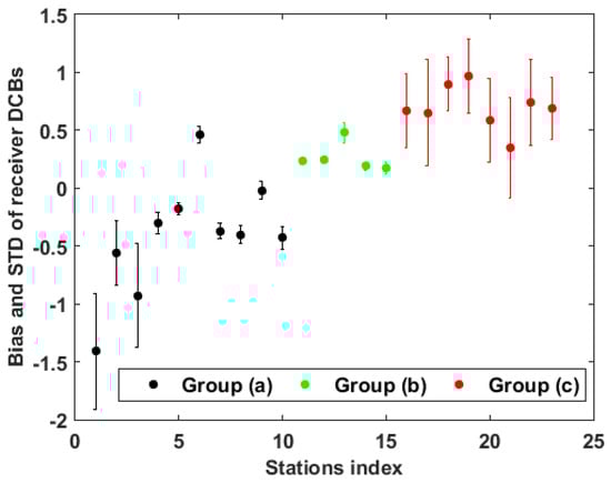
Figure 14.
Mean differences and STDs of receiver C2I-C6I DCB estimates between BDS2+BDS3 and BDS2-only solutions for the TRIMBLE NETR9 receiver.
Table 9.
Consistency of receiver DCBs between BDS2-only and BDS2+BDS3 solutions for the TRIMBLE NETR9 receiver (unit: ns).
To further research the impact of added BDS3 observations on the stability of receiver DCB estimates, we plotted the STD of the C2I-C6I receiver DCB estimates for the two solutions in Figure 15. As shown in the figure, the mean STDs of DCB estimates based on BDS2+BDS3 and BDS2-only solutions are 0.31 and 0.37 ns, respectively, indicting improved stability induced by the added BDS3 observations.
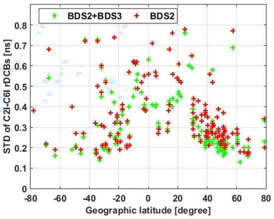
Figure 15.
STDs of receiver C2I–C6I DCB estimates at each station. The stations are aligned by geographic latitude on the horizontal axis.
To investigate the stability of the BDS3 receiver DCB estimates among the different frequency bands, the monthly STD of each individual receiver DCB estimates is shown in Figure 16. This figure shows that compared to the satellite-based STD values, the receiver DCBs show higher fluctuations. The STD values of receiver DCB estimates among the different frequency bands for all receivers located at low latitudes are larger than those of receivers located at other latitudes, indicating the latitudinal dependence of BDS3 receiver DCBs. The STDs of receiver DCBs between the B2I and B1C signals and other frequency bands are smaller than 0.4 ns and 0.6 ns, respectively, for most stations.
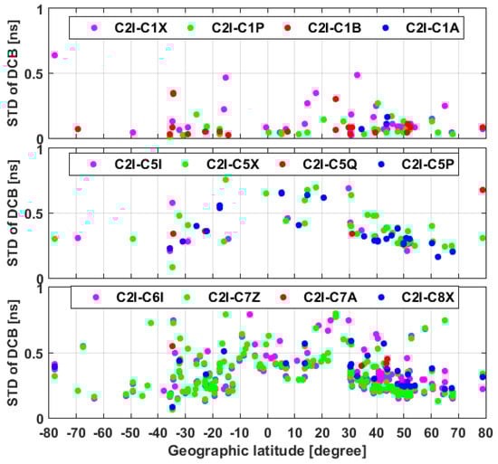
Figure 16.
Scatterplots of the STDs of BDS3 receiver DCB estimates versus geographic latitudes.
To study the impact of changes in types of receivers and antennas on receiver BDS DCB estimates, taking METG, SPT0 and YAR2 stations as examples, Figure 17 shows the time series of the receiver DCB estimates for the three stations during the test period. There are several gaps, due to discontinuous data or changes in the receiver hardware device. According to the information on the three receivers shown in Table 4, the receiver type for stations METG and YAR2 and the antenna type for station SPT0 changed during the period of DOY 218–227. The abnormal variations in receiver DCB estimates for the three stations are consistent with the changes in receiver hardware devices, from which we can conclude that the jumps are largely driven by changes in receiver type or antenna type. This justifies the impacts of changes in types of receivers and antennas on the variations in receiver DCB estimates.
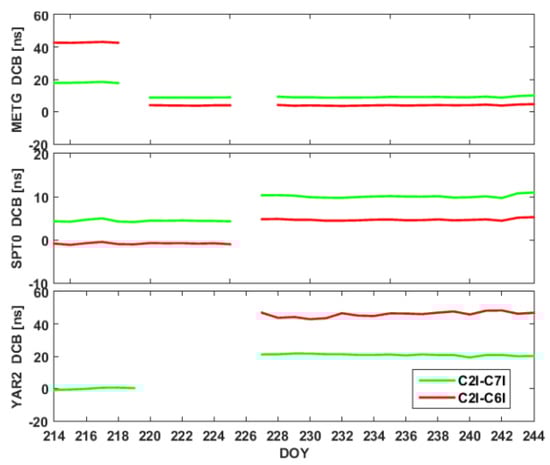
Figure 17.
Time series of daily DCB estimates at stations METG, SPT0 and YAR2 for DOY 214 to 244, 2020.
3.5. Performance of GIMs Estimated Using Only BDS Observations
To study the performance of the BDS in modeling the global ionospheric TEC, the GIMs that were produced based on BDS-only-obtained observational data were compared with the combined final GIM products of the IGS. In addition, GIMs based only on GPS data were also calculated, and used as a reference in the performance assessment of the BDS-based GIMs.
The bias and RMS series of the APM-based GIMs with regard to the combined final GIM products of the IGS during the period from DOY 214 to 244 in 2020 are shown in Figure 18. The figure depicts that the GPS-based GIM products provide better consistency with the IGS GIMs than do the BDS-based products. Taking the IGS-based GIM products as a reference, the accuracies of the BDS-based and GPS-based GIMs are 1.86 and 1.39 total electron content units (TECUs), respectively. Considering that the IGS-provided GIMs are calculated based on GPS and GLONASS data, the GPS-based GIMs are expected to be more consistent with the IGS GIM products than the BDS-based GIMs.
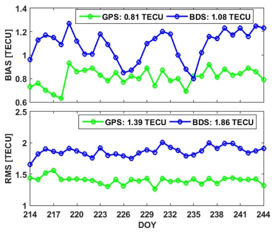
Figure 18.
Time series of the mean and RMSs of the differences between the estimates and the IGS-based GIMs during the period from DOY 214 to 244 in 2020.
The even distribution of ionospheric observables is recognized to play an important role in high-precision GIM product calculations. To study the impact of IPP distributions on the performance differences between the BDS-based and GPS-based GIMs, the IPP distributions of the BDS- and GPS-based ionospheric observables for the first 15 min of DOY 214, 2020 are shown in Figure 19. The density of the IPPs of the BDS is significantly increased when BDS3 satellites are included. Although the distributions of the IPPs tracked by both GPS and BDS satellites can cover most of the continuous regions, the IPPs for the GPS are denser than those of the BDS in the oceans. Thus, the poorer IPP distribution of BDS can be regarded as one of the reasons for the degraded precision of the BDS-based GIMs.
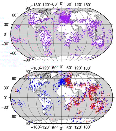
Figure 19.
Intersecting pierce point (IPP) distributions of the GPS (purple dot), BSD2 (red dot), and BDS3 (blue dot) ionospheric observables for the periods between UTC 00:00 and UTC 00:15 on DOY 214, 2020.
To investigate the performance of the BDS-based GIM in the position domain, the user positioning performance regarding single-frequency SPP has been analyzed using BDS observations from all accessible stations listed in Figure 2 for DOY 214–244, 2020. In the SPP process, we used only pseudorange observations and broadcasted navigation messages. The results of the positioning solutions without ionospheric error corrections were also analyzed. Moreover, the IGS-provided GIMs and the GIMs calculated using the APM method with only GPS data were also applied for a more comprehensive comparison. The RMS position errors of the SPP in the horizontal and vertical coordinate components, which were obtained for each 0.5-h bin over the test period with respect to local time, are illustrated in Figure 20. According to the mean values of the RMS errors summarized in the legend of this figure, the maximum differences in the horizontal and vertical position errors between the BDS-based GIMs and other GIMs products are less than 0.03 and 0.06 m, respectively. Compared to the results obtained without ionospheric error correction, the ionospheric correction obtained from the GIM products mainly reduces the SPP positioning bias in the Up component, showing a significantly better improved positioning accuracy in the vertical direction than in the horizontal direction.
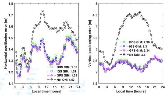
Figure 20.
Horizontal (left panel) and vertical (right panel) positioning errors with respect to local time during the period from DOY 214 to 244 in 2020.
4. Discussion
In this contribution, the characteristics of 13 types of BDS DCBs and the accuracy of BDS-based GIM are analyzed for the first time. The assessment proves that the contributed number of stations and observables has a large impact on both the stability of satellite DCB estimates and the performance of the GIMs. Thus, more receivers available to track BDS data should be developed to achieve more stable DCB estimates and better model the variation in the global ionospheric TEC.
The issue of whether there are code intersystem biases between BDS3 and BDS2 receiver DCBs is preliminarily analyzed in this study. Consistent with the study of Wang et al. [24], the difference between BDS2 and BDS2+BDS3 receiver DCBs is found to be related to the receiver type. Additionally, this study further found that the systematic bias is also related to the antenna type and firmware version. Although the average bias between the BDS2 and BDS3 receiver DCBs is close to 0, we still cannot draw the conclusion that there is no evident systematic bias between the BDS2 and BDS2+BDS3 receiver DCBs since the mean difference for JAVAD receivers reaches 1.03 ns. Therefore, the receiver DCBs of BDS3 and BDS2 should be separately estimated when BDS data collected by some specific types of receivers such as JAVAD receivers are processed.
The test in the SPP experiment shows that there are no significant differences between the GPS-and BDS-based GIMs in mitigating the ionospheric delay effects on position errors. Notably, when estimating the accuracy of ionospheric correction products, observation data during both high- and low-activity periods should be tested. However, BDS3 had not completed global constellation deployment until June 2020, which corresponded to low solar activity. Therefore, the BDS-based GIM validation in this study is based only on data collected during a low-solar activity period, in which the impact of the ionospheric delay was less than that during high-activity periods. More experiments based on data collected under high solar activity should be performed in the future.
5. Conclusions
This article provides an analysis of satellite and receiver DCBs among different frequency bands for BDS2 and BDS3, and an overview of the performance assessment of GIMs produced only by BDS observables for the first time. The GIMs and DCBs are estimated by the proposed APM method based on data obtained from the IGMAS and MGEX networks. In the proposed APM method, to improve the computational efficiency, GIMs based on BDS observations at the B1I, B2I and B3I signals are first estimated, and then the satellite and receiver DCBs among the other frequency bands are estimated by removing the ionospheric delay using the previously generated GIMs. The conclusions are summarized as follows:
- Good agreement of the APM-based BDS satellite DCB estimates with those of CAS and DLR is found, with RMS values of 0.26 and 0.18 ns, respectively. The mean STDs of the APM, DLR and CAS satellite DCB estimates are less than 0.1 ns. Larger differences between different DCB products are found for BDS3 than BDS2 satellites.
- For the BDS3 DCBs of the new signals, a close match of satellite DCB estimates between the same two frequency band signals is found.
- The BDS satellite DCB estimates among different frequency bands for IGSO satellites show better stability than those from MEO and GEO satellites for both BDS2 and BDS3. Additionally, the stability of BDS satellite DCB estimates is found to be related to the number of contributed stations and available observables applied in the process of DCB estimation.
- Variations in the types of receivers and antennas have impact on receiver DCB estimates. The systematic bias between BDS2 and BDS3 receiver DCBs is found to be related to the receiver type, antenna type and firmware version.
- The accuracies of GIMs based on BDS-only data and GPS-only data are 1.86 and 1.39 TECU, when taking the IGS-provided GIMs as references, and there is no significant difference in the positioning accuracy when the three GIM products are applied in SPP experiments during low solar activity periods.
Notably, the conclusion on the characteristics of satellite and receiver DCBs for the new BDS3 signals and the performance of GIMs based on only BDS data is drawn from the analysis based on data spanning only a month in 2020. More research should be performed with longer-term observations of BDS3 network satellites, and more evenly distributed BDS global stations in the future.
Author Contributions
M.L. provided the initial idea and wrote the manuscript; M.L. and Y.Y. designed and performed the research; Y.Y. helped with the writing and partially financed the research. All authors have read and agreed to the published version of the manuscript.
Funding
This work was supported by the National Key Research Program (No. 2016YFB0501900) and China Natural Science Funds (No. 42004027 and 41574033). The second author is supported by the Wang Kuancheng Pioneer Talents Project Lu Jiaxi International Team Program.
Data Availability Statement
The multi-GNSS observation data from the IGS MGEX networks are available at https://cddis.nasa.gov/archive/gps/data/daily/. The multi-GNSS broadcast ephemeris data are available at https://cddis.nasa.gov/archive/gnss/data/campaign/mgex/daily/rinex3/. The GIM products from IGS can be obtained at https://cddis.nasa.gov/archive/gnss/products/ionex/. The DCB products from CAS and DLR can be obtained at https://cddis.nasa.gov/archive/gnss/products/bias/.
Acknowledgments
The authors gratefully acknowledged the DLR and CAS for providing DCB products, the IGS and iGMAS for providing GNSS data, and the IGS for providing GIM products.
Conflicts of Interest
The authors declare no conflict of interest.
References
- Yang, Y.; Mao, Y.; Sun, B. Basic performance and future developments of BeiDou global navigation satellite system. Satell. Navig. 2020, 1, 1–8. [Google Scholar] [CrossRef]
- IGS_MGEX. Available online: https://mgex.igs.org/mgex/constellations/ (accessed on 15 January 2021).
- Yang, Y.; Xu, Y.; Li, J.; Yang, C. Progress and performance evaluation of BeiDou global navigation satellite system: Data analysis based on BDS-3 demonstration system. Sci. China Earth Sci. 2018, 61, 614–624. [Google Scholar] [CrossRef]
- Montenbruck, O.; Steigenberger, P.; Prange, L.; Deng, Z.; Zhao, Q.; Perosanz, F.; Romero, I.; Noll, C.; Stürze, A.; Weber, G.; et al. The Multi-GNSS Experiment (MGEX) of the International GNSS Service (IGS)—Achievements, prospects and challenges. Adv. Space Res. 2017, 59, 1671–1697. [Google Scholar] [CrossRef]
- Li, X.; Xie, W.; Huang, J.; Ma, T.; Zhang, X.; Yuan, Y. Estimation and analysis of differential code biases for BDS3/BDS2 using iGMAS and MGEX observations. J. Geod. 2018, 93, 419–435. [Google Scholar] [CrossRef]
- Li, M.; Yuan, Y.; Zhang, X.; Zha, J. A multi-frequency and multi-GNSS method for the retrieval of the ionospheric TEC and intraday variability of receiver DCBs. J. Geod. 2020, 94, 1–14. [Google Scholar] [CrossRef]
- Li, W.; Wang, G.; Mi, J.; Zhang, S. Calibration errors in determining slant Total Electron Content (TEC) from multi-GNSS data. Adv. Space Res. 2019, 63, 1670–1680. [Google Scholar] [CrossRef]
- Hernandez-Pajares, M.; Roma-Dollase, D.; Krankowski, A.; Garcia-Rigo, A.; Orus-Perez, R. Methodology and consistency of slant and vertical assessments for ionospheric electron content models. J. Geod. 2017, 91, 1405–1414. [Google Scholar] [CrossRef]
- Prol, F.D.; Camargo, P.D.; Monico, J.F.G.; Muella, M.T.D.H. Assessment of a TEC calibration procedure by single-frequency PPP. Gps Solut. 2018, 22, 35. [Google Scholar] [CrossRef]
- Roma-Dollase, D.; Hernández-Pajares, M.; Krankowski, A.; Kotulak, K.; Ghoddousi-Fard, R.; Yuan, Y.; Li, Z.; Zhang, H.; Shi, C.; Wang, C.; et al. Consistency of seven different GNSS global ionospheric mapping techniques during one solar cycle. J. Geod. 2017, 92, 691–706. [Google Scholar] [CrossRef]
- Ren, X.; Chen, J.; Li, X.; Zhang, X. Multi-GNSS contributions to differential code biases determination and regional ionospheric modeling in China. Adv. Space Res. 2020, 65, 221–234. [Google Scholar] [CrossRef]
- Li, M.; Zhang, B.; Yuan, Y.; Zhao, C. Single-frequency precise point positioning (PPP) for retrieving ionospheric TEC from BDS B1 data. GPS Solut. 2018, 23, 18. [Google Scholar] [CrossRef]
- Komjathy, A.; Sparks, L.; Wilson, B.D.; Mannucci, A.J. Automated daily processing of more than 1000 ground-based GPS receivers for studying intense ionospheric storms. Radio Sci. 2005, 40, 1–11. [Google Scholar] [CrossRef]
- Zhang, B.; Teunissen, P.J.G.; Yuan, Y.; Zhang, H.; Li, M. Joint estimation of vertical total electron content (VTEC) and satellite differential code biases (SDCBs) using low-cost receivers. J. Geod. 2017, 92, 401–413. [Google Scholar] [CrossRef]
- Liu, T.; Zhang, B.; Yuan, Y.; Li, Z.; Wang, N. Multi-GNSS triple-frequency differential code bias (DCB) determination with precise point positioning (PPP). J. Geod. 2018, 93, 765–784. [Google Scholar] [CrossRef]
- Guo, F.; Zhang, X.H.; Wang, J.L. Timing group delay and differential code bias corrections for BeiDou positioning. J. Geod. 2015, 89, 427–445. [Google Scholar] [CrossRef]
- Zhang, Y.; Chen, J.; Gong, X.; Chen, Q. The update of BDS-2 TGD and its impact on positioning. Adv. Space Res. 2020, 65, 2645–2661. [Google Scholar] [CrossRef]
- Dai, P.P.; Ge, Y.L.; Qin, W.J.; Yang, X.H. BDS-3 Time Group Delay and Its Effect on Standard Point Positioning. Remote Sens. 2019, 11, 1819–1847. [Google Scholar] [CrossRef]
- Wang, N.B.; Li, Z.S.; Montenbruck, O.; Tang, C.P. Quality assessment of GPS, Galileo and BeiDou-2/3 satellite broadcast group delays. Adv. Space Res. 2019, 64, 1764–1779. [Google Scholar] [CrossRef]
- CDDIS. Available online: https://cddis.nasa.gov/archive/gnss/products/bias/ (accessed on 15 January 2021).
- Montenbruck, O.; Hauschild, A.; Steigenberger, P. Differential Code Bias Estimation using Multi-GNSS Observations and Global Ionosphere Maps. Navigation 2014, 61, 191–201. [Google Scholar] [CrossRef]
- Wang, N.B.; Yuan, Y.B.; Li, Z.S.; Montenbruck, O.; Tan, B.F. Determination of differential code biases with multi-GNSS observations. J. Geod. 2016, 90, 209–228. [Google Scholar] [CrossRef]
- Li, M.; Yuan, Y.B.; Wang, N.B.; Li, Z.S.; Li, Y.; Huo, X.L. Estimation and analysis of Galileo differential code biases. J. Geod. 2017, 91, 279–293. [Google Scholar] [CrossRef]
- Wang, Q.; Jin, S.; Yuan, L.; Hu, Y.; Chen, J.; Guo, J. Estimation and Analysis of BDS-3 Differential Code Biases from MGEX Observations. Remote Sens. 2019, 12, 68. [Google Scholar] [CrossRef]
- Zhu, Y.; Tan, S.; Feng, L.; Cui, X.; Zhang, Q.; Jia, X. Estimation of the DCB for the BDS-3 new signals based on BDGIM constraints. Adv. Space Res. 2020, 66, 1405–1414. [Google Scholar] [CrossRef]
- Wang, Q.; Jin, S.; Hu, Y. Epoch-by-epoch estimation and analysis of BeiDou Navigation Satellite System (BDS) receiver differential code biases with the additional BDS-3 observations. Ann. Geophys Ger. 2020, 38, 1115–1122. [Google Scholar] [CrossRef]
- Gu, S.; Wang, Y.; Zhao, Q.; Zheng, F.; Gong, X. BDS-3 differential code bias estimation with undifferenced uncombined model based on triple-frequency observation. J. Geod. 2020, 94, 45. [Google Scholar] [CrossRef]
- Ciraolo, L.; Azpilicueta, F.; Brunini, C.; Meza, A.; Radicella, S.M. Calibration errors on experimental slant total electron content (TEC) determined with GPS. J. Geod. 2007, 81, 111–120. [Google Scholar] [CrossRef]
- Zhang, B.C.; Teunissen, P.J.G.; Yuan, Y.B.; Zhang, X.; Li, M. A modified carrier-to-code leveling method for retrieving ionospheric observables and detecting short-term temporal variability of receiver differential code biases. J. Geod. 2018, 93, 19–28. [Google Scholar] [CrossRef]
- Leick, A.; Rapoport, L.; Tatarnikov, D. GPS Satellite Surveying; Wiley: New York, NY, USA, 2015. [Google Scholar]
- Choi, B.-K.; Lee, S.J. The influence of grounding on GPS receiver differential code biases. Adv. Space Res. 2018, 62, 457–463. [Google Scholar] [CrossRef]
- Shi, C.; Fan, L.; Li, M.; Liu, Z.; Gu, S.; Zhong, S.; Song, W. An enhanced algorithm to estimate BDS satellite’s differential code biases. J. Geod. 2016, 90, 161–177. [Google Scholar] [CrossRef]


Publisher’s Note: MDPI stays neutral with regard to jurisdictional claims in published maps and institutional affiliations. |
© 2021 by the authors. Licensee MDPI, Basel, Switzerland. This article is an open access article distributed under the terms and conditions of the Creative Commons Attribution (CC BY) license (http://creativecommons.org/licenses/by/4.0/).