A Novel Unsupervised Classification Method for Sandy Land Using Fully Polarimetric SAR Data

Abstract

Classification based on polarimetric synthetic aperture radar (PolSAR) images is an emerging technology, and recent years have seen the introduction of various classification methods that have been proven to be effective to identify typical features of many terrain types. Among the many regions of the study, the Hunshandake Sandy Land in Inner Mongolia, China stands out for its vast area of sandy land, variety of ground objects, and intricate structure, with more irregular characteristics than conventional land cover. Accounting for the particular surface features of the Hunshandake Sandy Land, an unsupervised classification method based on new decomposition and large-scale spectral clustering with superpixels (ND-LSC) is proposed in this study. Firstly, the polarization scattering parameters are extracted through a new decomposition, rather than other decomposition approaches, which gives rise to more accurate feature vector estimate. Secondly, a large-scale spectral clustering is applied as appropriate to meet the massive land and complex terrain. More specifically, this involves a beginning sub-step of superpixels generation via the Adaptive Simple Linear Iterative Clustering (ASLIC) algorithm when the feature vector combined with the spatial coordinate information are employed as input, and subsequently a sub-step of representative points selection as well as bipartite graph formation, followed by the spectral clustering algorithm to complete the classification task. Finally, testing and analysis are conducted on the RADARSAT-2 fully PolSAR dataset acquired over the Hunshandake Sandy Land in 2016. Both qualitative and quantitative experiments compared with several classification methods are conducted to show that proposed method can significantly improve performance on classification.

1. Introduction

In recent years, desertification of grasslands has become increasingly severe due to continuous drought and grassland overload in Inner Mongolia Autonomous Region, China. According to research, Hunshandake Sandy Land, has become one of the main dust sources, so it is of great significance to monitor sandy land [1]. The development of spaceborne remote sensing technology and a massive increase in monitoring data provide many effective means to monitor the sandy land echo-environment [1,2]. The all-time all-weather features of active microwave synthetic aperture radar (SAR) are a particular advantage over optical sensors, and SAR can penetrate ground and vegetation with multi-polar observations [3,4]. The polarimetric SAR (PolSAR) which can obtain relatively complete polarimetric scattering information through four different channels (HH, HV, VH and VV) is referred to as a fully PolSAR [5]. Theory and practice show that the polarization feature of electromagnetic echoes is sensitive to the shape, texture, and other physical features of targets, and the differences in polarization signatures help distinguish different types of ground objects. Since radar response to sandy land is related to polarization, the exploitation of differences in polarization signatures for sandy land classification can improve accuracy with respect to polarization SAR data. Several PolSAR satellites have been launched to monitor the earth, including RADARSAT-1/2 (Canada), ALOS-1/2 (Japan), TerraSAR-X and Tandem-X (Germany), STR-C (NASA/JRL) (America), and GF-3 (China). Benefiting from the abundant PolSAR data acquired by these sensors, many classification applications have been reported in the literature [6,7,8,9,10].

The classification of PolSAR images can be divided into supervised and unsupervised methods, depending on whether the algorithm depends on a priori sample data [5]. The former needs human intervention to acquire prior knowledge, while the latter, in the absence of characteristic prior information, only uses scattering and statistical distribution information obtained from PolSAR data to perform image classification. Therefore, unsupervised classification is widely used to classify PolSAR images. Its process mainly includes two key steps. One is the choice of features which provides a basic basis for classification, so the expression of the selected features is the key to determining the performance of the classification results. The second is the design of classification algorithms. Although classical clustering algorithms have a complete mathematical theory as the basis, only reasonable use of them can achieve the ideal performance on classification, so the design of classification process is also a key when facing different study areas.

A widely used approach for obtaining polarimetric features is polarimetric target decomposition. It is the most effective way to understand polarimetric scattering mechanisms, which contributes significantly to identifying and classifying ground targets [11]. Polarization target decomposition method can be categorized as either from the perspective of incoherent decomposition: (1) the eigen-decomposition-based approach with quantitative analysis of eigenvectors and eigenvalues of coherency or covariance matrix; (2) the model-based decomposition with models representing physical scattering phenomena. Model-based decomposition has developed rapidly, since Freeman–Durden proposed three-component decomposition in 1998 [12,13,14,15,16,17,18,19,20,21,22,23,24,25]. In this method, three scattering models (surface, double-bounce, and volume scattering) are defined, and three polarimetric parameters with distinct physical interpretations corresponding to the three models are derived. These scattering components constitute the characteristics for sandy land classification. However, the pioneer model-based decomposition methods have a major flaw regarding the emergence of negative power. To solve this problem, Cloud [6] proposed a hybrid Freeman/Eigenvalue decomposition method, in which surface scattering is orthogonal to secondary scattering. Singh [13] extended the volume scattering model and combined it with the rotation transformation of the coherence matrix, by which the negative power is overcome with improved decomposition accuracy. Other methods have been proposed [14,15,16,17,18,19,20], such as to employ orientation angle compensation (OAC) and phase angle rotation (PAR) to improve decomposition performance, and accordingly improve classification accuracy [21]. We propose an alternative new hybrid Freeman/eigenvalue decomposition method based on adaptive model-based to obtain polarimetric features.

Classification algorithms can be categorized as pixel-wise and region-based [26]. Pixel-wise algorithms focus on the processing of a single pixel, while neglecting the similarity between adjacent pixels belonging to the same type of target [27]. Thus, it is difficult to extract structural information of a homogeneous region and keep the edge information and spatial structure of the image [28]. Region-based methods can effectively consider spatial correlation between pixels in a local region, which contributes to the improved performance of PolSAR image classification. One of the most widely used strategies for region-based methods is image segmentation. The basic principle of segmentation is merging the adjacent and homogeneous pixels into the same region, and the heterogeneous pixels are divided into different regions. Finally, the image is segmented into many small homogeneous regions with similar sizes. In recent years, various PolSAR image segmentation algorithms have been proposed [29,30,31,32,33,34,35,36,37]. Among them, Simple Linear Iterative Clustering (SLIC) [32] is a simple and effective segmentation algorithm for natural images, which has been successfully applied for PolSAR images [25,29,33,34]. The algorithm can generate superpixels with compact regions, relatively uniform sizes, and maintain the region boundaries. In this paper, the PolSAR image is segmented by Adaptive Simple Linear Iteration Clustering (ASLIC), and the image is divided into different region blocks. These area blocks are used as the input sample points of the spectrum clustering algorithm. Compared with directly using the original image, the amount of data processing is greatly reduced, the problems of insufficient memory and slow processing speed are improved [35]. Furthermore, as for clustering algorithms, such as k-means and expectation maximization (EM), must assume a convex spherical sample space, and they tend to fall into local optima [23,24,25,26]. Fortunately, the spectral clustering algorithm, which is based on graph theory, can transform clustering into a graph partitioning problem. It is carried out by k-means clustering in a projection space, in which the transformation matrix is calculated by eigenvectors of Gaussian similarity matrix of samples [24]. Such methods are attracting considerable attention in the field of polarized SAR processing.

In this study, Hunshandake Sandy Land stands out for its vast area of sandy land, a great variety of ground objects, and a complex, intricate structure with irregular characteristics compared with conventional land cover types. In order to mitigate the problem and improve final classification accuracy, starting from the two key steps of unsupervised classification, an unsupervised classification method based on new decomposition and large-scale spectral clustering with superpixels (ND-LSC) is proposed. Figure 1 depicts the proposed architecture. There are two essential parts for the classification method. The first part is the extraction of polarized scattering power by ND which contribute significantly to understand the polarimetric scattering mechanisms of sandy land. The second part is the large-scale spectral clustering (LSC), which is a classification algorithm based on regional level. The algorithm, i.e., scattering power as input vs superpixels as basic unit, is tested on the sandy land. Specifically, we utilize the advantages of new decomposition to extract polarization scattering power (m_s, m_d, and m_v), which is used to construct the feature vector X = [m_s, m_d, m_v], and then superpixels are generated by the ASLIC algorithm when the feature vector combined with the spatial coordinate information are employed as input, followed by spectral clustering to complete the classification.

There are several advantages of the proposed method. The main novel contributions of this work are:

Firstly, it is a classification structure for areas with vast area, variety of ground objects and intricate structure.

Secondly, these two aspects are crucial to complete the final classification through spectral clustering. On the one hand, the new decomposition method helps to interpret the polarization scattering characteristics of ground objects. On the other hand, the classification algorithm takes the superpixel as the unit. In LSC, it can make full use of the polarization information and spatial information of the target to generate superpixels. These two aspects are crucial to complete the final classification through spectral clustering.

The structure of this paper is organized as follows. In Section 2, the descriptions of the Hunshadake Sandy Land and parameters of RADARSAT-2 fully PolSAR were presented. Then, the details of the proposed ND-LSC unsupervised classification are introduced in Section 3, and the flowchart of the method is given at the end of this section. In Section 4, on the one hand, the classification performance of ND-LSC and other classification methods are compared. On the other hand, it analyzed the influence of decomposition parameters and superpixels segmentation on classification result. Finally, discussion and conclusions are drawn in Section 5 and Section 6, respectively.

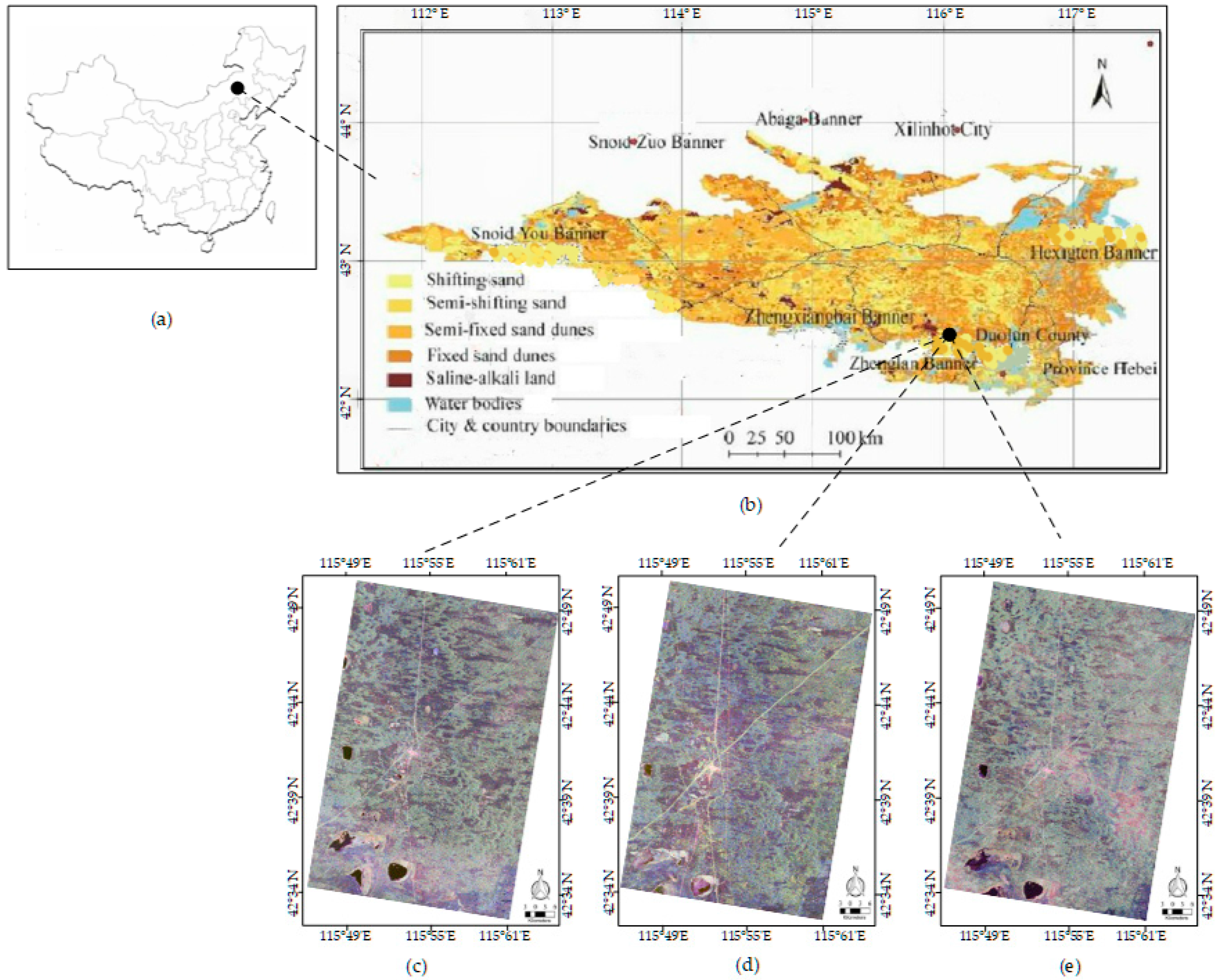
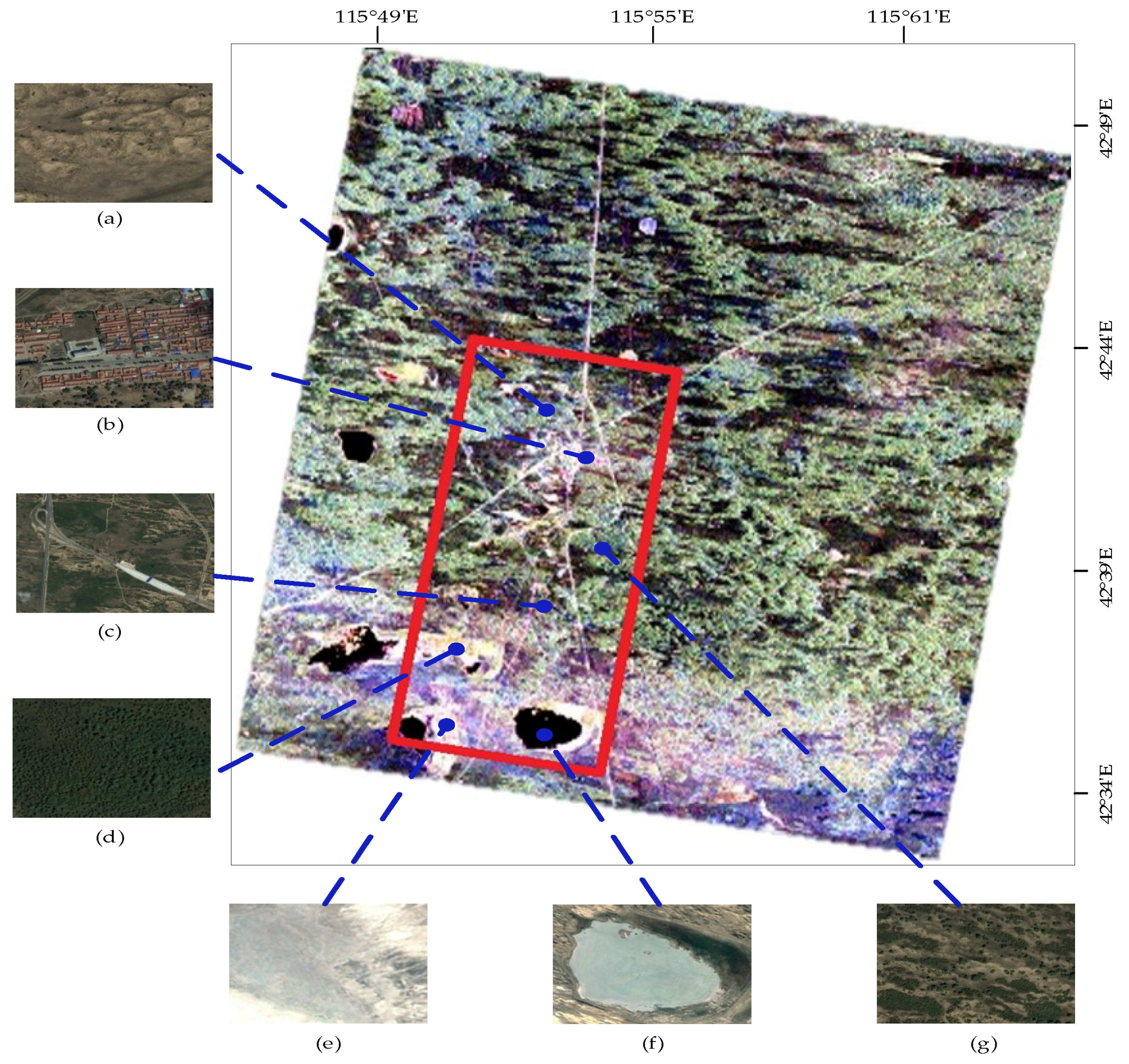
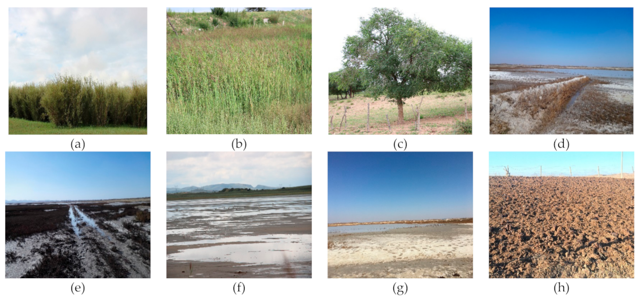
2. Study Area

Hunshandake Sandy Land, is located at 42°32′–42°50′ N, 115°49′–116°12′ E in the south of Xilingol League, Inner Mongolia, China. It is a semi-temperate grassland with a semi-arid continental climate. The altitude ranges from 1150 to 1500 m rising slowly from northwest to southeast. The edge of the sandy land is hilly and denuded, and there are dunes, basins, lakes, and denuded plateaus in this area. Sand dunes can be divided into fixed, semi-fixed, and mobile dunes from the perspective of vegetation coverage. The vegetation of fixed dunes is mainly herbaceous, and the proportions of irrigation are relatively high. Semi-fixed sand dunes distributed among fixed sand dunes always present speckle shapes in SAR images. A mobile sand dune can move, as the effect of the wind for the surface vegetation is rare. There are five types of sandy land in the area. Fixed sand accounts for 29.23%, semi-fixed sand for 29.52%, mobile sand for 15.23%, semi-mobile sandy land for 23.27%, and saline-alkali land for only 2.55%. There is almost no Gobi sand in Hunshandake Sandy Land [35], as shown in Figure 2a. Polarimetric SAR data are obtained from the RADARSAT-2 satellite, with data parameters as shown in

Table 1. The Parameters of RADARSAT-2 fully PolSAR.

Parameters	Statement
Wave mode	Fine quad polarization
Polarization types	HH VV HV VH
Sampling pixel spacing	~4.73 m
Sampling line spacing	~4.94 m
Pass direction	Descent
Ellipsoid name	WGS 84

. The corresponding PolSAR images are shown in Figure 2b–d. According to surveys, three main types of phenomena occur or have occurred in Hunshandake Sandy Land: (1) soil and water are severely lost, (2) the degree of desertification increases, and (3) grass pasture is severely degraded. Therefore, it is urgent to constantly monitor the change of grassland features. The data used in this article were collected in September 2013, August 2016, and September 2017.

Hunshandake Sandy Land is famous for its unique characteristics, such as a large area, various types of features, and intricate structures. As shown in Figure 3, the details of seven typical features.

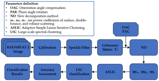
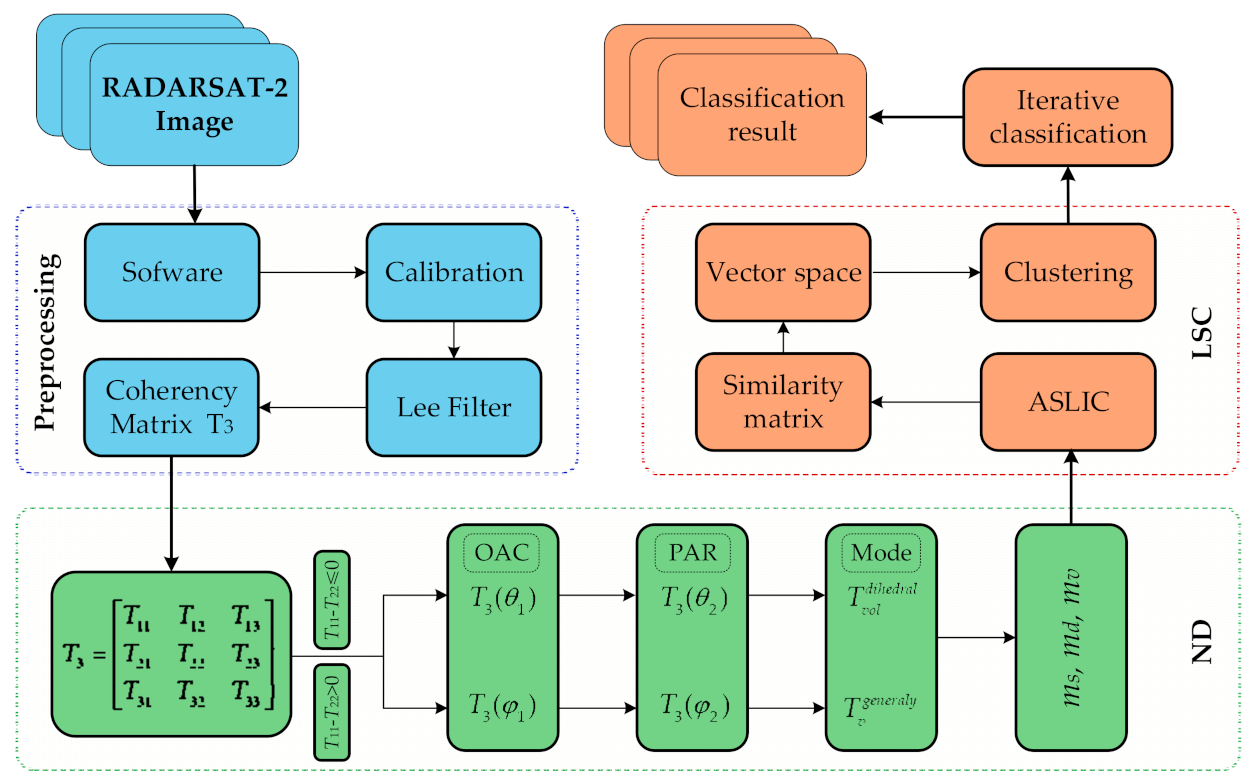
3. Methodology

An unsupervised classification method combined with new decomposition and large-scale spectral clustering with superpixels is proposed for Hunshadake Sandy Land classification. The method consists of data preprocessing, new decomposition (ND), superpixel segmentation by adaptive simple linear iterative clustering (ASLIC), and large-scale spectral clustering (LSC) classification. The workflow of the proposed ND-LSC is shown in Figure 4. The polarization parameters (m_s, m_d, m_v) are more accurately extracted from the ND, which is used to construct the feature vector X = [m_s, m_d, m_v]. The application of LSC is more in line with the characteristics of its large area. The feature vector X and spatial coordinate information constitute the input vector of ASLIC, which is used to generate superpixels. Representative points are selected from superpixels, and the bipartite graph between the representative points is formed. According to the principle of the spectral clustering algorithm, the classification of PolSAR is completed. It can be seen from the flowchart that the classification method has two three parts, (1) extracting polarization parameters from decomposition (2) spectral clustering with superpixels. We propose improvements from these two aspects to classify the sandy land.

3.1. Data Preprocessing

The SAR pre-processing procedure is performed in three steps with SARscape software (PolSARpro 5.3.0). These include calibration, registering, and filtering. The PolSAR single look complex (SLC) image data can be geometrically calibrated and registered by the NEST tool. Then the Lee filter is used to suppress inherent speckle noise, and the corresponding polarimetric coherency matrix T₃ for every pixel of data is generated. Finally, the area of interest is selected.

As for fully PolSAR image, the acquired scattering matrix in H-V polarization basis can be written as [5]:

$$S=\left[\begin{array}{cc}{S}_{HH}& S_{HV}\\ S_{VH}& S_{VV}\end{array}\right]$$

(1)

where the different elements in matrix S represent the backscattering coefficients of the different polarimetric channels. S_HH and S_VV are the common-polarized echo channels, and S_HV and S_VH are the cross-polarized echo channels. According to the reciprocity principle, the two cross-polarizations are considered equal, that is, S_HV = S_VH, and the scattering target vector obtained from the matrix S can be expressed as follows:

$$\overline{K}=\frac{1}{\sqrt{2}}{\left[\begin{array}{ccc}{S}_{HH}+S_{VV}& S_{HH}-S_{VV}& 2S_{HV}\end{array}\right]}^{†}$$

(2)

Then the corresponding coherency matrix is (3) [11]:

T₃ contains nine independent parameters, which is relevant to the physical properties of the observed targets. Generally speaking, T₁₁ is relevant to surface scattering mechanism, T₂₂ is relevant to double-scattering mechanism, and T₃₃ is relevant to volume scattering mechanism. T₁₃ is relevant to cross-polarization power generated by the coupling between surface and volume scattering mechanisms. T₂₃ is relevant to cross-polarization power generated by the coupling between double-bounce and volume scattering mechanism. Elimination of the cross-polarization power cannot only optimize the PolSAR coherency matrix T₃, but can help approach the reflection symmetry condition.

$$\begin{array}{cc}{T}_3& =〈\overline{K}•{\overline{K}}^H〉\to \left[\begin{array}{ccc}{T}_{11}& T_{12}& T_{13}\\ T_{21}& T_{22}& T_{23}\\ T_{31}& T_{32}& T_{33}\end{array}\right]=\left[\begin{array}{ccc}〈{\left|k_1\right|}^2〉& {\displaystyle \langle }{k}_1{k}_2^{\ast }{\displaystyle \rangle }& {\displaystyle \langle }{k}_1{k}_3^{\ast }{\displaystyle \rangle }\\ {\displaystyle \langle }{k}_2{k}_1^{\ast }{\displaystyle \rangle }& 〈{\left|k_2\right|}^2〉& {\displaystyle \langle }{k}_2{k}_3^{\ast }{\displaystyle \rangle }\\ {\displaystyle \langle }{k}_3{k}_1^{\ast }{\displaystyle \rangle }& {\displaystyle \langle }{k}_3{k}_2^{\ast }{\displaystyle \rangle }& 〈{\left|k_3\right|}^2〉\end{array}\right]\hfill \\ & =\left[\begin{array}{ccc}〈{\left|S_{HH}+S_{VV}\right|}^2〉& {\displaystyle \langle }\left(S_{HH}+S_{VV}\right){\left(S_{HH}-S_{VV}\right)}^{\ast }{\displaystyle \rangle }& 2{\displaystyle \langle }\left(S_{HH}+S_{VV}\right)S_{HV}^{\ast }{\displaystyle \rangle }\\ {\displaystyle \langle }\left(S_{HH}-S_{VV}\right){\left(S_{HH}+S_{VV}\right)}^{\ast }{\displaystyle \rangle }& 〈{\left|S_{HH}-S_{VV}\right|}^2〉& 2{\displaystyle \langle }\left(S_{HH}-S_{VV}\right)S_{HV}^{\ast }{\displaystyle \rangle }\\ 2{\displaystyle \langle }{S}_{HV}{\left(S_{HH}+S_{VV}\right)}^{\ast }{\displaystyle \rangle }& 2{\displaystyle \langle }{S}_{HV}{\left(S_{HH}-S_{VV}\right)}^{\ast }{\displaystyle \rangle }& 4〈{\left|S_{HV}\right|}^2〉\end{array}\right]\end{array}$$

(3)

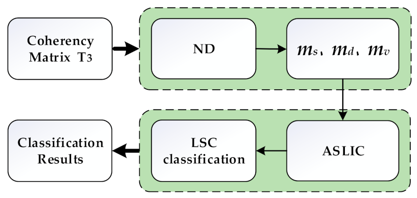
3.2. New Decomposition

In order to effectively obtain the polarization parameters of Hunshandake Sandy Land to improve the final classification results, a new decomposition is presented based on [7,17] in this paper. The decomposition eliminates cross-polarization at the bottom power to reduce the influence of the volume scattering overestimation problem, followed by the hybrid Freeman/Eigenvalue decomposition based on adaptive model to extract the polarization scattering power.

3.2.1. Removal

Orientation angle compensation (OAC) [15,16] and phase angle rotation (PAR) [18] are common polarimetric target decomposition data processing methods. They are used to remove T₂₃ and T₁₃, which can increase the power of the common polarization term, decrease the power of the cross-polarization term, minimize the influence of different orientation angles on polarimetric decomposition results, Thus, the coherency matrix T₃ is rotated as follows:

$$T_3({\phi }_1)=R({\phi }_1)T_3{T}_3{({\phi }_1)}^{\ast T}$$

(4)

$$T_3({\phi }_2)=R({\phi }_2)T_3({\phi }_1)T_3{({\phi }_2)}^{\ast T}$$

(5)

where *T denotes complex conjugation and transposition, and the rotation matrices R(φ₁) and R(φ₂) are given by [21]:

$$\begin{array}{cc}\hfill R({\phi }_1)& =\left[\begin{array}{ccc}\cos 2{\phi }_1& 0& \sin 2{\phi }_1\\ 0& 1& 0\\ -\sin 2{\phi }_1& 0& \cos 2{\phi }_1\end{array}\right]\hfill \\ \hfill {\phi }_1& =\frac{1}{4}{\tan }^{-1}\left[\frac{2\mathrm{Re}\left(T_{13}\right)}{T_{11}-T_{33}}\right]\hfill \end{array}$$

(6)

$$\begin{array}{l}R({\phi }_2)=\left[\begin{array}{ccc}\cos 2{\phi }_2& 0& \mathrm{j}\sin 2{\phi }_2\\ 0& 1& 0\\ \mathrm{j}\sin 2{\phi }_2& 0& \cos 2{\phi }_2\end{array}\right]\\ {\phi }_2=\frac{1}{4}{\tan }^{-1}\left[\frac{2\mathrm{Im}\left(T_{13}\right)}{T_{11}\left({\phi }_1\right)-T_{33}\left({\phi }_1\right)}\right]\end{array}$$

(7)

After this rotation, the eliminated T₁₃ of coherency matrix T₃ can be eliminated by Equations (4) and (5) completely.

After OAC, the real part of T₁₃ becomes zero, and its imaginary part can be set to zero via PAR [21], that is,

$$\begin{array}{c}{T}_{11}\left({\phi }_2\right)=T_{11}({\phi }_1){\cos }^{2}2{\phi }_2+T_{33}({\phi }_1){\sin }^{2}2{\phi }_2\\ +\mathrm{Im}\left(T_{13}({\phi }_1)\right)\sin 4{\phi }_2\\ T_{22}\left({\phi }_2\right)=T_{22}\\ T_{13}\left({\phi }_2\right)=0\end{array}$$

(8)

Similarly, T₂₃ represents a cross term of double-bounce and volume scattering, which can be completely eliminated by OAC and PAR, that is,

$$\begin{array}{c}{T}_{11}\left({\theta }_2\right)=T_{11}\\ T_{22}\left({\theta }_2\right)=T_{22}({\theta }_1){\cos }^{2}2{\theta }_2+T_{33}({\theta }_1){\sin }^{2}2{\theta }_2\\ +\mathrm{Im}\left(T_{23}({\theta }_1)\right)\sin 4{\theta }_2\\ T_{23}\left({\theta }_2\right)=0\end{array}$$

(9)

The rotation matrices R(φ₁) and R(φ₂) are given by [18]. The choice of rotation transformation depends on the form of the dominant scattering mechanism. It can be determined according to the value of $T_{11}-T_{22}$, which contributes to removing the maximum of the cross-polarization power generated by the coupling between common polarization and the cross-polarization scattering mechanism. The coherent matrix after two unitary rotations is as follows:

$$T_3{}^{\prime }=\left\{\begin{array}{c}[T_3({\phi }_2)]\\ [T_3({\theta }_2)]\end{array}\right.\begin{array}{c}\\ \end{array}\begin{array}{c}{T}_{11}-T_{22}>0\\ T_{11}-T_{22}\le 0\end{array}$$

(10)

3.2.2. Adaptive Model-Based Decomposition

After two unitary rotations, the coherency matrix T₃’ can be decomposed as follows:

$$T_3{}^{\prime }=m_s{T}_s+m_d{T}_d+m_v{T}_v$$

(11)

where T_s, T_d and T_v are scattering models of surface, double-bounce, and volume scattering, respectively, with corresponding power coefficients m_s, m_d and m_v.

The surface scattering model T_s and double-bounce scattering model T_d are represented by eigenvectors, and can be expressed as follows [13]:

$$\begin{array}{cc}{T}_s& =\left[\begin{array}{ccc}{\cos }^2{\alpha }_s& \cos {\alpha }_s\sin {\alpha }_s{e}^{i{\phi }_s}& 0\\ \cos {\alpha }_s\sin {\alpha }_s{e}^{-i{\phi }_s}& {\sin }^2{\alpha }_s& 0\\ 0& 0& 0\end{array}\right]\end{array}$$

(12)

$$T_d=\left[\begin{array}{ccc}{\cos }^2{\alpha }_d& \cos {\alpha }_d\sin {\alpha }_d{e}^{i{\phi }_d}& 0\\ \cos {\alpha }_d\sin {\alpha }_d{e}^{-i{\phi }_d}& {\sin }^2{\alpha }_d& 0\\ 0& 0& 0\end{array}\right]$$

(13)

where α_s and α_d depend on the two dielectric constants of the surface, reflector and the angle of incidence, and α_s < π/4, α_d > π/4. φ_s and φ_d are the scattering phases for surface scattering and double-bounce scattering mechanisms, respectively. Under the conditions α_s + α_d = π/2 and φ_d − φ_s= ±π, these two components T_s and T_d have orthogonality with each other. This reduces the number of unknowns in (11), which can be rewritten as:

$$T_3=T_{sd}+T_v$$

(14)

The adaptive volume scattering model is the main distinction of improved hybrid decomposition, and can be described as follows:

$$T_v=\left[\begin{array}{ccc}{V}_{11}& V_{12}& 0\\ V_{21}& V_{22}& 0\\ 0& 0& V_{33}\end{array}\right]$$

(15)

The object is judged to be located at artificial area when double-bounce scattering is dominant scattering mechanisms. Under the condition, we consider this physical situation in more detail and assume for more accurate modeling that volume scattering mainly comes from the dihedral structure of the artificial target. The model is expressed as follows [13]:

$$T_{vol}^{dihedral}=\frac{1}{15}\left[\begin{array}{ccc}0& 0& 0\\ 0& 7& 0\\ 0& 0& 8\end{array}\right]$$

(16)

The object is judged to be located in a natural area when surface scattering is dominant. At this time, volume scattering mainly comes from a cloud of randomly oriented dipole scatter such as vegetation, in which case we adopt the generalized volume scattering model [16]:

$$\begin{array}{l}{T}_v^{generaly}=\\ \frac{1}{\frac{3}{2}(\gamma +1)-\frac{\sqrt{\gamma }}{3}}\left[\begin{array}{ccc}\frac{\gamma +1}{2}+\frac{\sqrt{\gamma }}{3}& \frac{\gamma -1}{2}& 0\\ \frac{\gamma -1}{2}& \frac{\gamma +1}{2}+\frac{\sqrt{\gamma }}{3}& 0\\ 0& 0& \frac{\gamma +1}{2}-\frac{\sqrt{\gamma }}{3}\end{array}\right]\end{array}$$

(17)

where $\gamma =〈{\left|S_{HH}\right|}^2〉/〈{\left|S_{VV}\right|}^2〉$, and $\gamma$ is the ratio of the horizontal and vertical polarization components.

To determine the scattering power coefficients of m_v, m_s and m_d, first the volume scattering power m_v coefficient is calculated as [17]:

$$m_v=V_{33}/T_{33}$$

(18)

Then, Equation (14) can be written as follows:

$$T_{sd}=T_3-T_v$$

(19)

Finally, the remaining scattering power coefficient m_s and m_d can be calculated as the eigenvalues of remainder matrix T_sd on the basis of dominant scattering mechanism (${\lambda }_{1sd}>{\lambda }_{2sd}$). In case of T₁₁ − T₂₂ > 0, m_s and m_d can be determined as:

$$\begin{array}{ccc}{m}_s={\lambda }_{1sd}& and& m_d={\lambda }_{2sd}\end{array}$$

(20)

In the case of T₁₁ − T₂₂ < 0, m_s and m_d can be determined as:

$$\begin{array}{ccc}{m}_s={\lambda }_{2sd}& and& m_d={\lambda }_{1sd}\end{array}$$

(21)

3.3. LSC Classification

Spectral clustering algorithms usually involve two large steps (1) to construct a similarity matrix (2) to solve the corresponding eigenvalue problem on the Laplace. However, accounting for the particular surface features of the Hunshandake Sandy Land, the implementation of the algorithm requires a lot of memory and affects the classification accuracy. Therefore, on the basis of obtaining the polarization scattering parameters (m_s, m_d, m_v), this paper generates representative points through superpixels, and subsequently a sub-step of representative points selection as well as bipartite graph formation, followed by the spectral clustering algorithm to complete the classification task.

3.3.1. Superpixels Segmentation

The ASLIC algorithm is utilized to generate superpixels in this paper, and it is developed based on the SLIC algorithm. The basic principle of SLIC is to use k-means for segmentation in a local area. In the beginning, some seeds are uniformly selected on the image plane at intervals Ns as the initial clustering center of the superpixels. The formula for the distance between a pixel and its adjacent superpixel region in the PolSAR image is generally expressed as [32]:

$$D_{SLIC}=\sqrt{d_W(S_i,S_{pi})+\beta \ast {\left(\frac{d_{XY}(i,j)}{N_s}\right)}^2}$$

(22)

where d_xy is the Euclidean distance between the image plane coordinate points i and j, and $d_W$ the Wishart distance. Since the Wishart distance may be negative, it is not a good distance measure. In this paper, Wishart distance will be replaced by Bartlett distance as:

$$d_W(S_i,S_{pi})=\ln \left|{{\displaystyle \sum }}_j\right|+Tr({{\displaystyle \sum }}_j^{-1}{T}_i)$$

(23)

where T_i and ∑_j are the respective sample coherence matrices of pixel S_i and superpixel region S_pi. Polarization parameters (m_s, m_d, m_v) can be extracted more accurately from ND, and are used to construct the vector X= [m_s, m_d, m_v] as the feature vector of the coherence matrix.

Since the values of $d_W$ and $d_{XY}$ changes with different images, and also with regions, $D_{SLIC}$ is modified to adaptively balance the distance between the pixel values and the distance in the image plane space, and Equation (22) can be modified as follows:

$$D_{SLIC}=\sqrt{\frac{d_w(S_i,S_{pi})}{{\max }_{S_i\in S_{pi}}{d}_W(S_i,S_{pi})}+\beta \ast {\left(\frac{d_{XY}(i,j)}{N_S}\right)}^2}$$

(24)

The ranges of the two items in Equation (24) are very similar, and it is easy to determine the contribution of the two components. Consequently, ASLIC with the advantage of adaptive distance formula is selected to generate superpixel in this paper.

3.3.2. LSC Classification

The idea of spectral clustering algorithms is derived from the theory of spectral graph partitioning. If a dataset is regarded as a set of all vertices in a graph, and the weights of edges between vertices represent the similarities between data, then spectral clustering is a method to divide the graph by a weight. Then, to find the optimal solution of the graph partitioning criterion becomes the essential problem of spectral clustering. According to the Rayleigh–Ritz theory, several eigenvectors of similarity matrix W are optimal partition-approximate solutions. That is, the original optimal segmentation problem is converted to the spectral decomposition of the similarity matrix or Laplacian matrix. Therefore, the key to classification for a PolSAR image based on spectral clustering is to obtain the similarity matrix W, expressed as follows [25]:

$$W_{ij}=\exp \left(-\frac{d(s_i,s_j)}{2{\sigma }^2}\right)$$

(25)

where s_i, s_j are sample of data; d(s_i, s_j) is the distance between superpixel, and usually is the Euclidean distance; and $\sigma$ is a scale parameter. We construct a normalization Laplacian matrix L_rw by similarity matrix W as [32]:

$$L_{rw}=D^{-1}L=I-D^{-1}W$$

(26)

where L = D − W, and D is the degree matrix, which consists of the corner elements of W.

Based on the symmetric Wishart distance measure as Equation (23), the similarity matrix of spectral clustering can be defined as shown:

$$W_{ij}^T=\exp \left(-\frac{d_w(T_{Pi},T_{Pj})}{2{\sigma }^2}\right)$$

(27)

where T_pi and T_pj are the coherency matrix of superpixels (p_i, p_j), and d_w is the symmetric Wishart distance.

The similarity matrix of spectral clustering based on central features can be defined as shown:

$$W_{ij}^F=\exp \left(-\frac{d(F_{Pi},F_{Pj})}{2{\sigma }^2}\right)$$

(28)

where F_pi and F_pj are the central features vector (X = [m_s, m_d, m_v]) of superpixels (p_i, p_j), and d is the cosine distance.

The similarity matrix Z for LSC is defined as follows:

$$Z_i{}_j=\left\{\begin{array}{cc}1& i=j\\ W_{ij}^T\ast W_{ij}^F& i\ne j\end{array}\right.$$

(29)

The procedure of the LSC in this paper can then be described as follows:

• Segment the PolSAR image into superpixels with ASLIC.
• Calculate the mean values of (m_s, m_d, m_v) in each superpixel region to form representative points.
• Calculate similarity matrix Z between representative points and Laplacian matrix L_rw.
• Calculate eigenvectors corresponding to the first K largest eigenvalues of matrix L_rw as a matrix Q = [q₁, q₂, … q_k].
• Normalize matrix Q with Equation (24).
• Cluster the row vectors of normalization matrix V with k-means.

The similarity matrix between representative points is calculated with LSC, which constructs a bipartite graph to decrease the memory and increase the speed of PolSAR image processing. For natural sandy land of complex characteristics, such as a large area, irregular objects [38,39], various features and intricate structures, LSC can be performed efficiently and flexibility. Moreover, the spatial information is effectively loaded with the help of superpixel segmentation algorithm, which further improves the final classification effect.

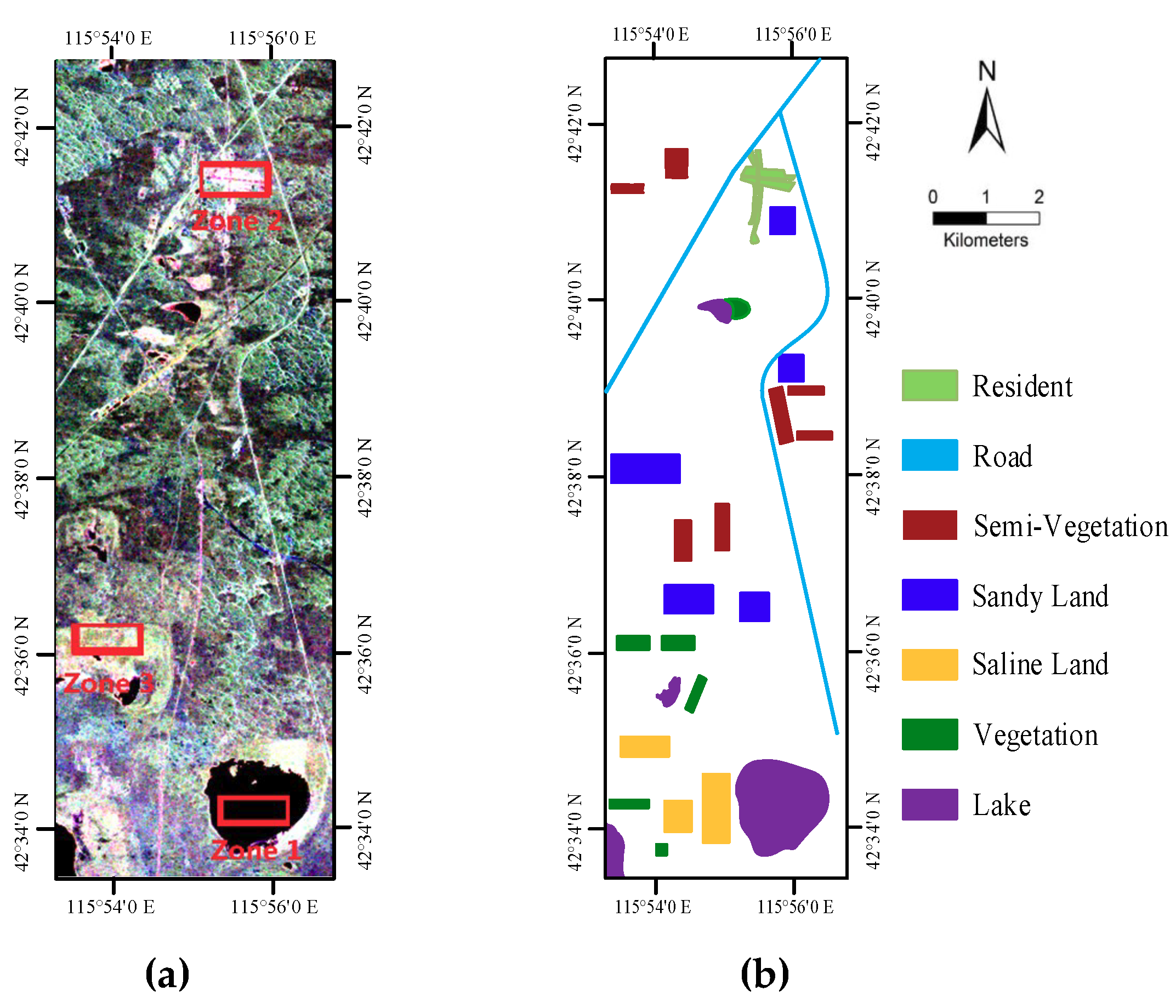
4. Experimental Results

As described in Section 2, there are various and complex types of features in the sandy land. Therefore, the area in the red color box is taken as the study area. The area is 1000 × 3000 pixels, mainly including residents (RT), roads (RD), semi-vegetation sand (SS), sandy land (DL), saline land (SL), vegetation (V), and lakes (L). The Pauli RGB image after Lee filtering is shown in Figure 5a. Test samples without overlap (i.e., from different fields) are randomly selected, as shown in Figure 5b, to evaluate the classification methods. The detailed information is shown in

Table 2. Collected field data and number of pixels under test.

Land Cover	Number of Pixels	Number of Fields
Residents(RT)	23,088	1
Roads(RD)	44,291	2
Semi-vegetation Sand(SS)	84,291	7
Sandy Land(DL)	127,600	5
Saline Land(SL)	43,600	3
Vegetation(V)	28,925	6
Lakes(L)	137,320	4

.

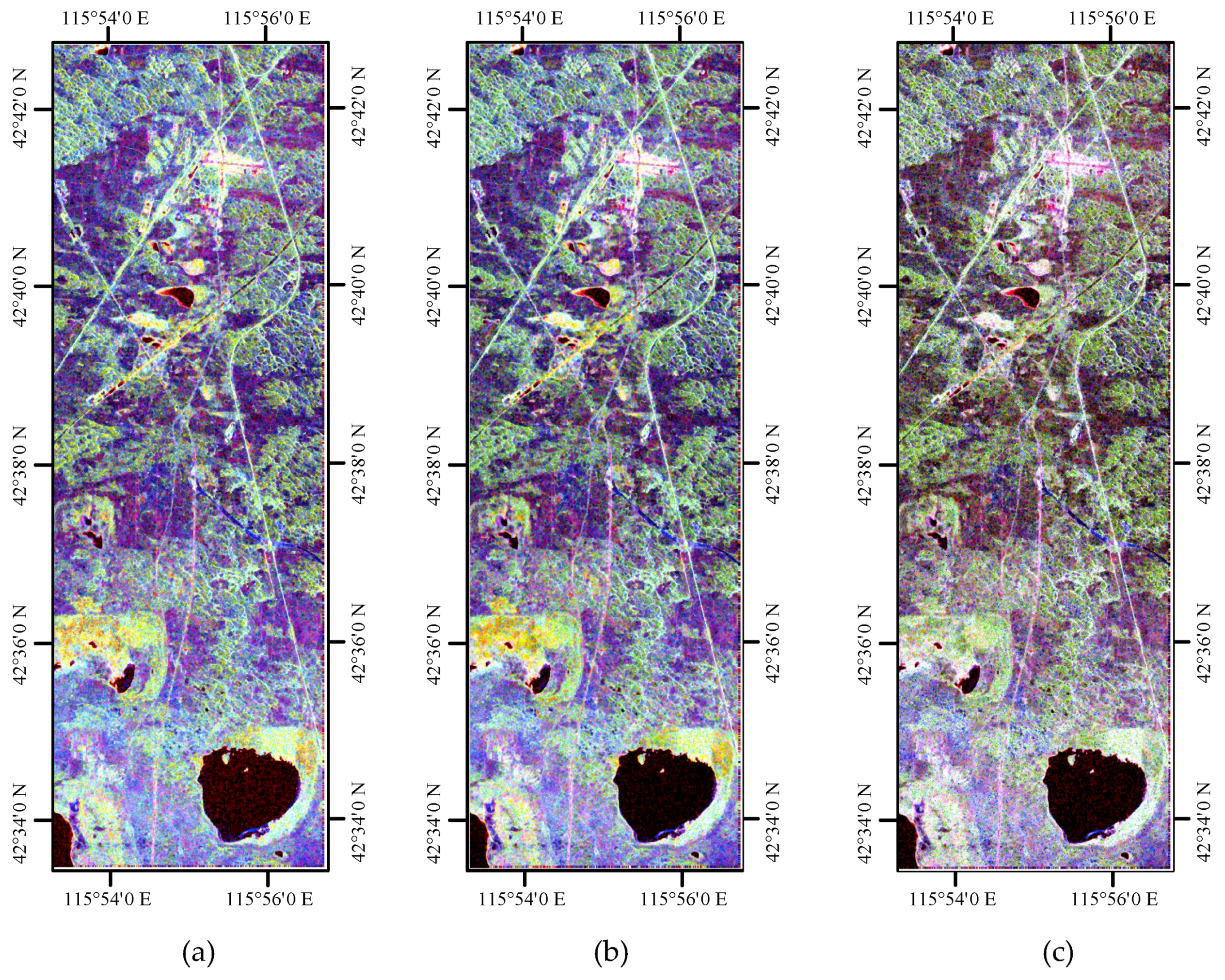
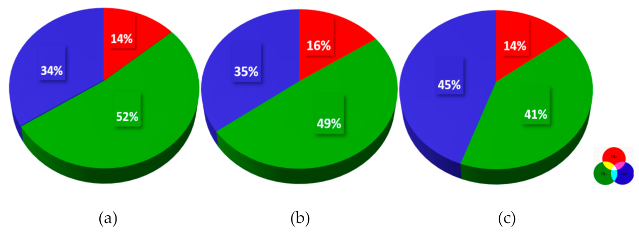
4.1. Decomposition Results

Three decomposition approaches are adopted to study area decomposition, and investigated to determine which is more suitable. The first strategy is to adopt original hybrid Freeman/eigenvalue decomposition (HFED) [7]. The second is to utilize HFED with extended volume scattering (HFEDE), which is surely more reasonable than the first strategy. The extend volume scattering are applied to the ensemble average of dipole scatters or dihedral (horizontal or vertical) corner reflectors. The third approach is to use the ND, as described in Section 3. In 3.2.1 of Section 3, the cross-polarization scattering components of the PolSAR data are removed by OAC and PAR, which solves the problem that the arrangement direction of the building is not parallel to the radar azimuth direction. In 3.2.2 of Section 3, volume scattering mainly comes from the dihedral structure of the artificial target for more accurate modeling in artificial areas, while it comes from a cloud of randomly oriented dipole scatter such as vegetation in natural areas. The decomposition results obtained under the above three approaches are shown in Figure 6. At a glance, it is difficult to see the differences of the three images. Therefore, the three decomposition approaches corresponding to the percentage of the power values of the three polarization scattering powers (m_s, m_d, m_v) are shown in Figure 7, from which it can be seen that the volume scattering power ratio decreases from 52% with HFED to 41% using ND as proposed in this paper. At the same time, the ratio of surface scattering increases to 45%, which accords with the actual scattering characteristics of the region, and double-bounce scattering increases from 14% with HFED to 16% with HFEDE. Finally, the results of the decomposition approach more accurately reflect the scattering characteristics of real objects.

For further analysis, three zones are selected and marked by red rectangles in Figure 5a and labeled Zone 1, Zone 2, and Zone 3. Each zone is 100 × 240 pixels, and the types of ground truth for these zones are lake areas, residents, and trees, respectively. It is well known that the dominant scattering powers of these three zones are surface, double-bounce, and volume, respectively, as shown in

Table 3. Mean Values of Dominated Scattering Powers in Selected Zones.

	Mean_ms (Zone 1)	Mean_md (Zone 2)	Mean_mv (Zone 3)
HFED	0.867	0.518	0.828
HFEDV	0.869	0.547	0.790
ND	0.988	0.604	0.710

. In Zone 1, it can be seen that mean_m_s as given by ND is 0.988, which is about 13.6% higher than for the other two approaches. In residential areas, because buildings and the ground constitute a large number of dihedral structures, double bounce scattering is dominant. In Zone 2, ND again performs best. Specifically, mean_m_d from the proposed method is 0.604, which exceeds the mean values of HFED and HFEDE by 16.6% and 10.4%, respectively. However, in Zone 3, mean _ mv with HFED is the largest. In the ND, the cross-polarization power contributes to all of the three scattering models, which leads to the surface scattering power and double-bounce scattering power being higher than those generated by the current hybrid Freeman/eigenvalue decomposition techniques. On the whole, ND obtains better decomposition performance than the other methods.

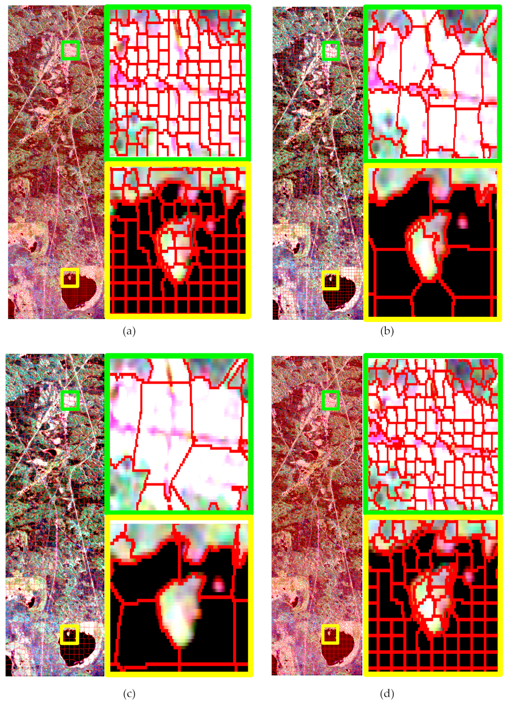
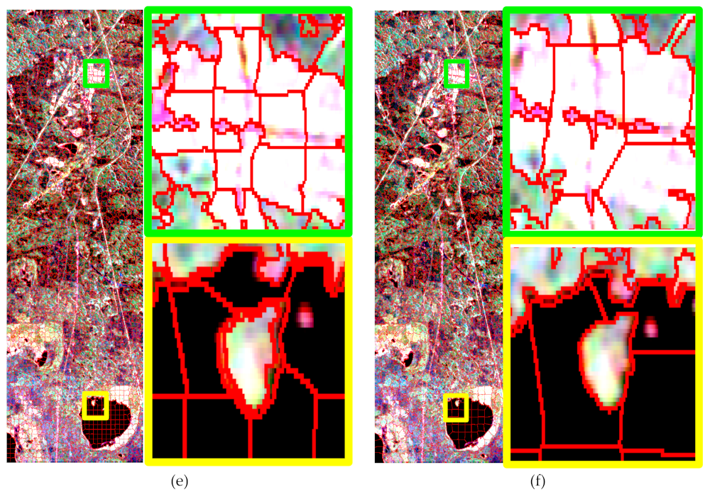
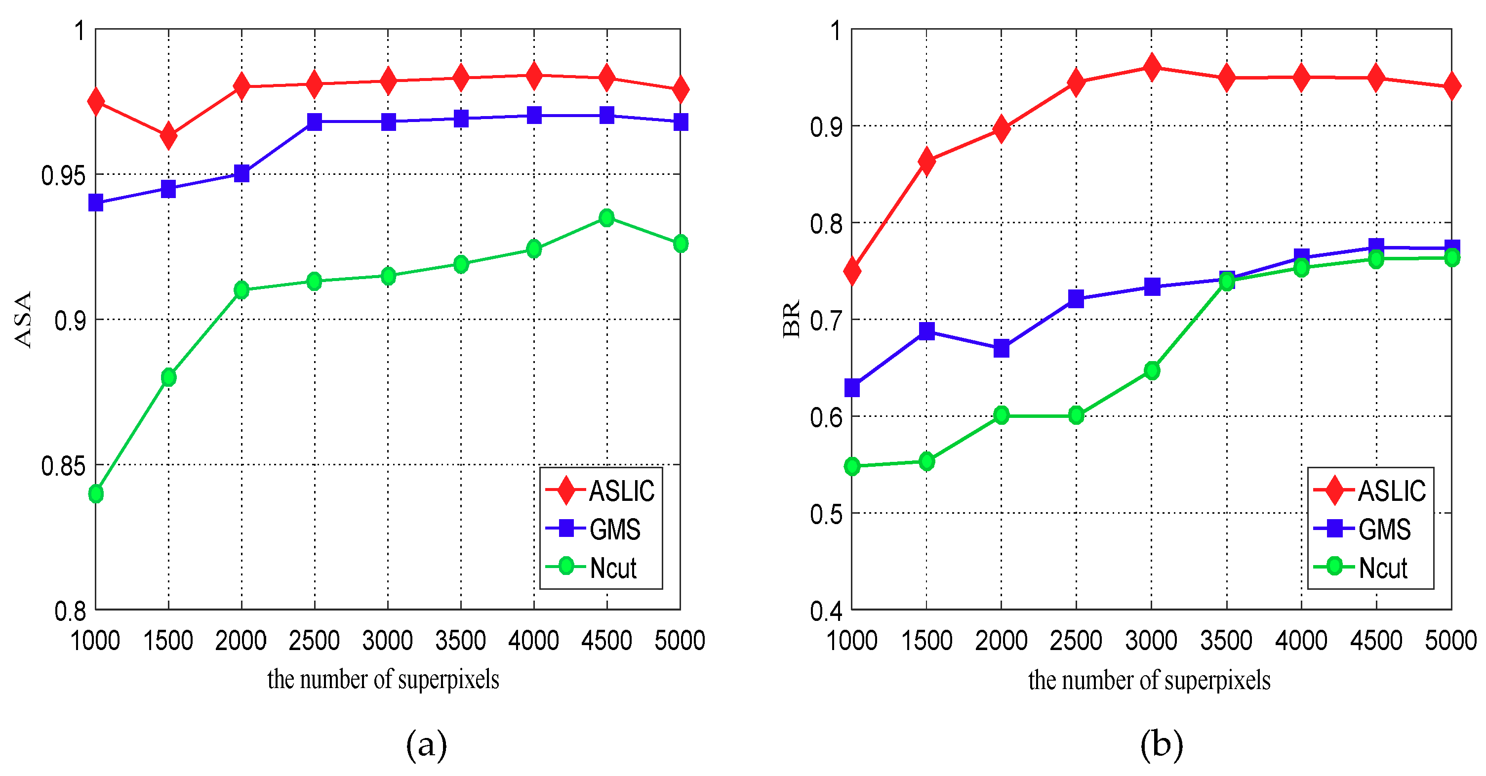
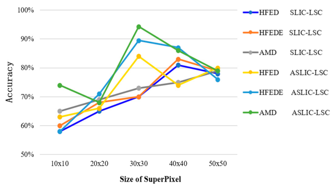
4.2. Superpixels Generation Results

Two adjustable parameters related to the ASLIC algorithm are introduced in 3.3 of Section 3. The parameter β is used to balance the distance between the pixel value and the distance in the image plane space, and it usually has a fixed value of 1. N_s is used to control the superpixel size of a block. This determines the similarity matrix Z, which affects the accuracy of the final classification result. At the same time, to produce better superpixel segmentation results, we test the segmentation effect when N_s is 10, 30, and 50. The superpixel generation maps are shown in Figure 8. From the magnified view of the region in the box, we can see that ALSIC shows better boundary-preserving ability than SLIC for superpixel generation of PolSAR images, especially for some narrow or smaller targets. Specifically, the structures of target can obviously be observed after superpixels segmentation works with N_s = 30, including good detail in the island and building areas. Compared with Figure 8b,e shows better segmentation quality, as the sizes of superpixels are similar, the borders of superpixels are smoother, and the edges of the island and building areas are preserved well. So, ASLIC outperforms SLIC for superpixel segmentation results under the same parameter N_s.

To illustrate the superiority of ASLIC in superpixel generation of PolSAR image, we compare the performances of the ASLIC with generalized mean shift (MS) [30] and Ncut [30], and evaluate the performances of the superpixels by boundary recall (BR) [27] and achievable segmentation accuracy (ASA) [27]. BR represents the degree of maintains between superpixels and real boundaries. ASA indicates the degree of coincidence between superpixels and real targets. Figure 9 shows the ASA scores and the BR scores. As the number of superpixels increases, the performance of each algorithm is basically improved until it is relatively stable. Due to the complex terrain type, the gap between the ASA score and the BR score of these three methods are large to each other. However, ASLIC has the highest ASA score and BR score. It improves the BR score at 4000 superpixels to 95.0%, which is 17.6% and 18.7% higher than GMS and Ncut, respectively. At same time, the ASA score of ASLIC is the highest. Hence, we can conclude that the superpixel by ASLIC algorithm is suitable for the study area of Hunshandake Sandy Land.

4.3. Classification Results

In this section, the classification results corresponding to three methods are shown in Figure 10, which includes the results of unsupervised classification based on HFED and spectral clustering with superpixels of [33] (HED-SC), unsupervised classification based on the use of Neumann decomposition and Random Forest Classifier (ND-RF), and the proposed classification method (ND-LSC). We adopt the overall accuracy (OA) and Kappa coefficient to evaluate the performance of different methods. Accuracy is calculated by Equation (30):

$$\begin{array}{cc}OA=\frac{TN}{NG},& Kappa=\frac{OA-P_e}{1-P_e}\end{array}$$

(30)

where TN is the number of correct classifications for all the training samples and NG is the total number of pixels in ground truth, P_e represents the proportion of misinterpretation caused by accidental factors in the interpretation of remote sensing images. For each class, user’s accuracies (UA) and producer’s accuracies (PA) explained in Equation (31) are also calculated [27].

$$\begin{array}{cc}PA=\frac{TP}{TP+FP},& UA=\frac{TP}{TP+FN}\end{array}$$

(31)

where TP is the true positive or the number of correctly detected class points, FP is the false positive or the number of incorrectly detected class points, and FN is the false negative.

The classification accuracies of these three classification methods are listed in

Table 4. Confusion Matrix of the ND-LSC Method.

Class	HED-SC		ND-RF		ND-LSC
	PA (%)	UA (%)	PA (%)	UA (%)	PA (%)	UA (%)
RT	81.17	95.19	85.42	73.64	90.22	96.94
RD	89.05	64.51	91.35	68.69	98.75	95.45
SS	91.31	84.28	93.45	85.36	94.62	87.28
DL	87.82	89.64	86.19	90.39	93.21	87.13
SL	81.69	94.37	84.67	94.75	91.02	87.07
V	75.20	90.54	79.89	94.47	97.87	69.65
L	96.35	99.67	96.86	99.68	98.07	74.59
OA (%)	89.68		90.02		95.22
Kappa	0.8717		0.9205		0.9404

. It can be observed that the proposed method outperforms the others. On the one hand, the OA of the proposed method is 95.22%, while the values of the other two methods are 89.68% and 90.02%, respectively. ND-LSC has the best kappa coefficient (0.9404). On the other hand, for six out of seven classes, the proposed method performs better than ND-RF. For vegetation, the classification precision improves up to from 79.89% for HED-SC to 97.87% for the proposed method. In addition, for each class, the proposed method obtains better UA. In summary, our approach performs better on complex terrain classification.

The findings in [11] also show that the parameters from the various polarimetric decompositions benefit the overall accuracy of classification methods. Polarimetric decompositions represent the scattering mechanisms of natural environments by scattering models. For the dominant scattering mechanism from different decomposition, the LSC scheme is able to better pick out small differences in the signal that characterizes the different classes. The violin plots introduced in Figure 11 illustrate three scattering mechanisms based on HFED, and ND decomposition shows differentiation between classes. Where Figure 11a,b show the distribution of the double-bounce scattering power coefficient m_d found within each class, Figure 11c,d show the distribution of the surface scattering power coefficient m_s found within each class Figure 11e,f show the distribution of the volume scattering power coefficient m_v found within each class. It can be seen that the m_d values from the HFED shows little differentiation between classes compared from the ND, which is generally associated with the double-bounce mechanism. However, the classes with the lowest UA and PA are the SL, which have significant overlap in double-bounce scattering, as seen in Figure 11a,b. In addition, for distribution of power coefficients m_v and m_s, compared with ND decomposition, the scattering mechanism based on HFED shows that the differences between classes are relatively small. In summary, the polarization parameters from ND benefit to the better performance of LSC classification in the sandy land.

To further illustrate the effectiveness of the proposed approach, six classification strategies are implemented to discuss the impact of accuracy indices (%) with different superpixels sizes. The parameter N_s ranges from 10 to 50, with an interval of 10. Figure 12 displays the experiment results. It can be seen that almost every classification strategy has the highest accuracy when N_s = 30. The classification accuracy of ND-SLIC-LSC exceeds those of HFED-SLIC-LSC and HFEDE-SLIC-LSC, because ND more accurately obtains the polarization scattering power (m_s, m_d, m_v). HFED-ASLIC-LSC has better classification accuracy than HFED-SLIC-LSC; because ASLIC generates superpixels, it has a stronger adaptation ability, and selection of spatial features is acquired to greatly improve classification accuracy. Thus, the proposed ND-ASLIC-LSC has the best accuracy—more than 94%.

Based on above discussions, several conclusions can be draw from experimental results. On the one hand, the proposed method (ND_LSC) obtains the best performance seen as OA (95.41%) and Kappa coefficient (0.943) in two categories of experiments, ie, it can better obtain a higher OA and Kappa coefficient by taking full advantage of the polarimetric features and spatial information. On the other hand, the performance using ND strategy is better than other decomposition strategies resulting from scattering powers (m_s, m_d and m_v) can be extracted more efficiently through the ND strategy. Secondly, the application of LSC is more in line with characteristics of its large area. The feature vector X combined with spatial coordinate information constitutes the input vector of ASLIC, which is used to generate superpixels.

To fully understand the consistency of classification results with real features, a field survey was conducted with Sangendalai town as the center. Several major types of land cover are selected for further analysis. Real photographs of land cover are shown in Figure 13, including vegetable I, vegetable II, semi-vegetation sand, lake I, lake II, saline land I, saline land II, sandy land I, sandy land II, road I, road II, and residents. The ground truth is used as a reference for the analysis of classification results. The geographic locations corresponding to the latitude and longitude of different land covers are recorded and displayed in

Table 5. Latitude, longitude, and sampling time of different features.

Location	Longitude and Latitude	Land Cover
1	115°56′52″ E 42°42′23″ N	Vegetable I
2	115°56′17″ E 42°42′12″ N	Vegetable II
3	115°55′25″ E 42°42′1″ N	Semi-vegetation Sand
4	115°54′21″ E 42°35′57″ N	Lake I
5	115°55′46″ E 42°35′9″ N	Lake II
6	115°54′21″ E 42°35′57″ N	Saline Land I
7	115°54′39″ E 42°35′47″ N	Saline Land II
8	115°59′9″ E 42°43′2″ N	Sandy Land I
9	115°57′58″ E 42°41′39″ N	Sandy Land II
10	115°56′2″ E 42°41′58″ N	Road I
11	115°56′22″ E 42°39′41″ N	Road II
12	115°56′2″ E 42°41′58″ N	Residents

. We compare the actual land cover with the result of the proposed classification method. It can be seen that Figure 13a,b show both types of vegetation, which correspond to two test samples in the green area. The green dense area represents vegetation II, and the sparse area represents vegetation I in Figure 10c. Most of the saline-alkali land is distributed around the lake by observing Figure 13d–g. Correspondingly, the yellow area surrounds the purple in Figure 10c. There are two typical roads in Figure 13j,k, one surrounded by buildings and the other by vegetation. It can be seen from Figure 10c that some light blue thin lines cross areas and surround light green areas. Some light-blue blocks are seen by the lake. This phenomenon will be discussed below.

5. Discussion

We have proposed an unsupervised classification method (ND-LSC), which combines the advantages of the ND strategy, the ASLIC algorithm, and the LSC algorithm. The experimental results in Hunshandake Sandy land manifested that the proposed method accomplishes the best performances with regard to OA and Kappa. This is mainly attributed to two aspects. On the one hand, an ND strategy method is adopted to extract polarimetric scattering powers (m_s, m_d and m_v), which contribute to superpixels being more reasonably generated by the ASLIC algorithm. On the other hand, the unsupervised classification-based LSC algorithm calculates the similarity matrix between representative points of superpixels generated by the ASLIC algorithm, which constructs a bipartite graph to solve the problem of insufficient memory and slow speed for PolSAR image processing. The following points in the experimental results are worth discussing.

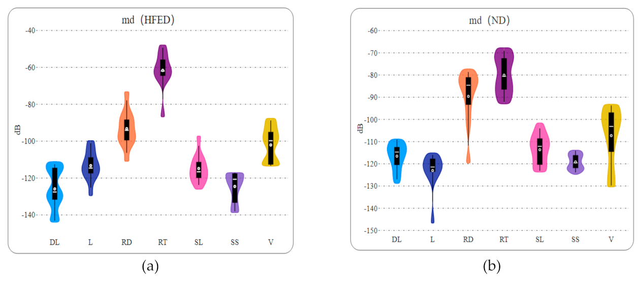
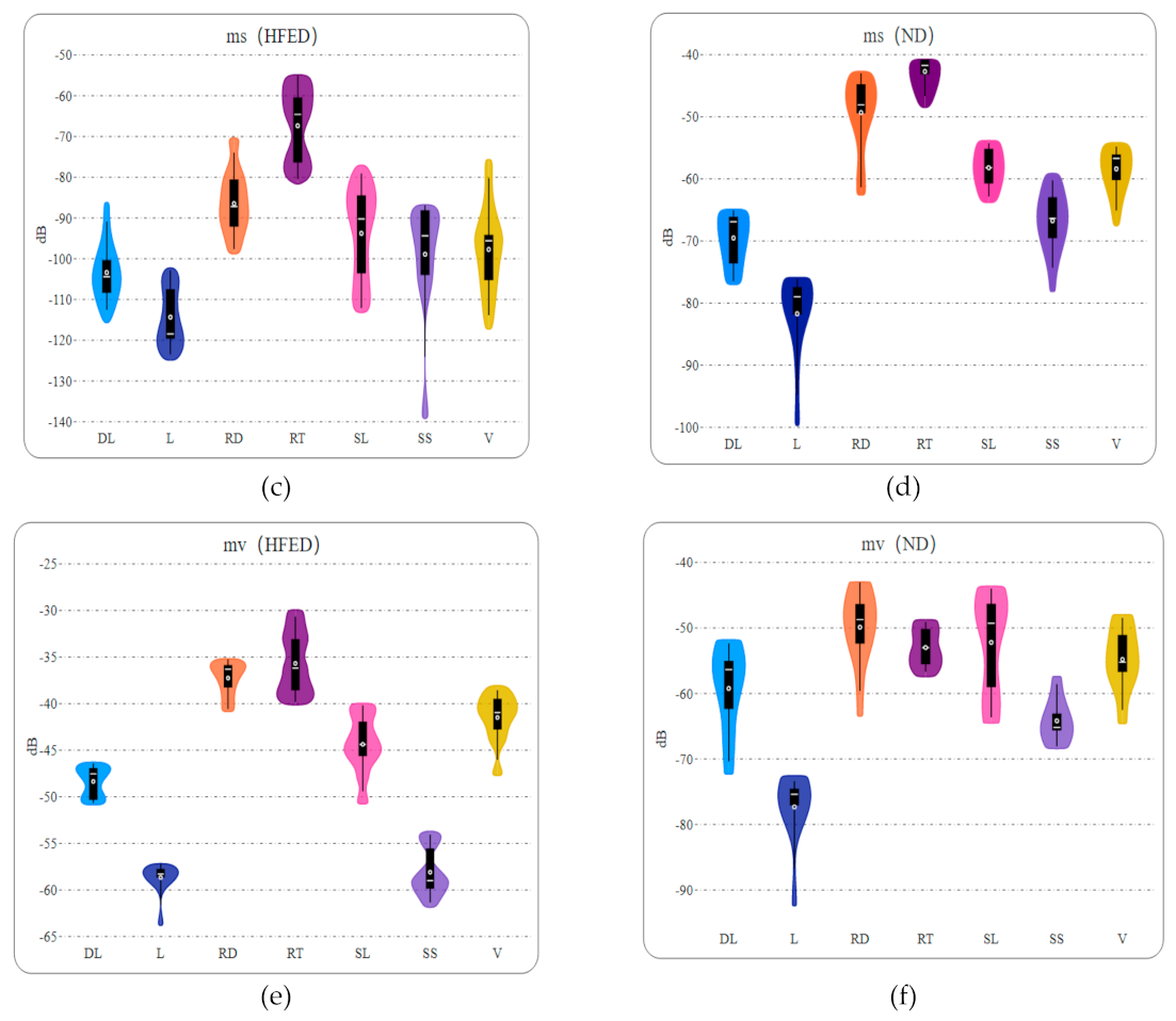
• ND strategy can more effectively obtain polarization parameters than other decomposition strateges. There are two main reasons for this phenomenon. One is that the traditional decomposition strategy has a better performance for PolSAR imagery in other fields, but the characteristics of Hunshandake Sandy land are not very ideal. Another reason is that OAC and PAR are not performed and volume scattering models cannot adapt to the environment in natural and artificial areas during decomposition, which affects the decomposition result. After OAC and PAR strategy, which enhances the T₁₁ and T₂₂ elements of coherence matrix T₃ power. Among them element T₁₁ is relevant to surface scattering mechanism; element T₂₂ is relevant to double-scattering mechanism. In other words, classes dominated by surface scattering and double-scattering mechanism can be classify accurately. Therefore, the polarization parameters extracted by ND strategy can be utilized to generate superpixels in Hunshandake Sandy land.
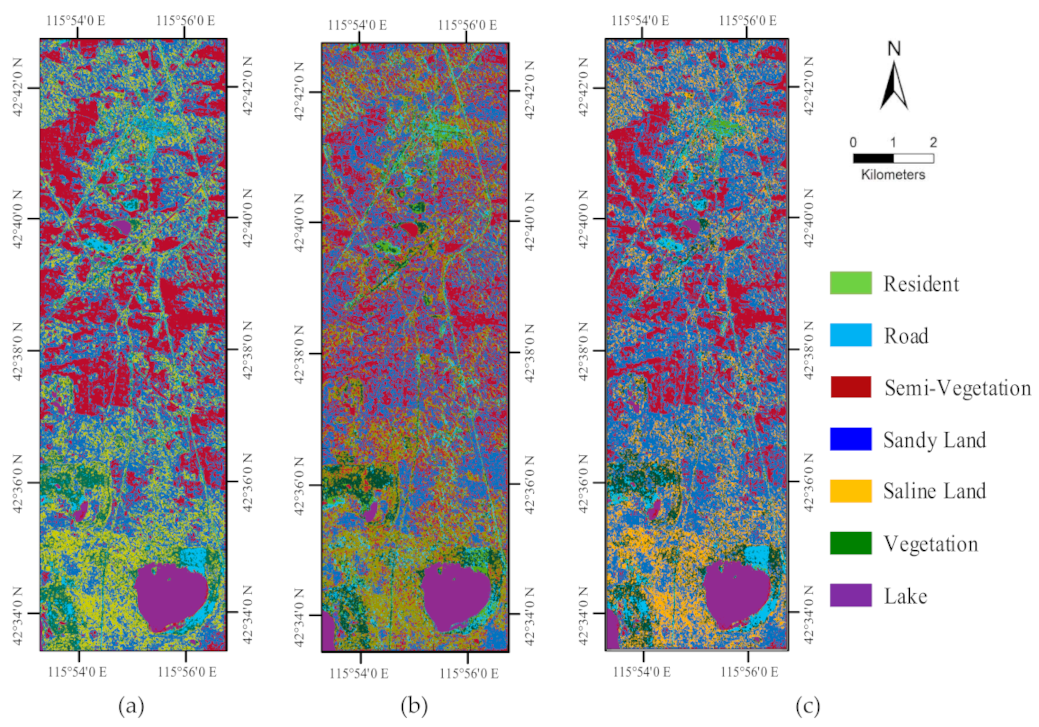
• There are the details that cannot be ignored of the classification result in Figure 10b, the obvious thing that can be observed is the road area around the lake. This phenomenon is not commission errors, classifying areas that are not roads as roads. This could be put down to the fact that both classes are predominantly surface scattering (water surface and roads surface) with relatively low surface roughness. The ground is very smooth after some small lakes degraded, which makes very similar to scattering mechanism of road. This would indicate that this specific environment has a polarimetric signature that could be associated with many classes.

However, there still are some disadvantages in the proposed method: (1) the algorithm structure is relatively complex and time-consuming when compared with conventional unsupervised classification methods. (2) This method has relative limitations and currently has a good classification result in the Hunshandake sandy land.

6. Conclusions

We have proposed an unsupervised classification method for Hunshandake Sandy Land. It integrates three key steps: the new decomposition (ND), superpixels segmentation, and the LSC algorithm. We have analyzed the capabilities of these steps to improve classification performance. Specifically, three classification methods and six classification strategies are discussed and applied to evaluate their effectiveness and feasibility. The analysis shows that the proposed method has superior classification performance on OA (95.41%) and kappa coefficient (0.943). Three years of data from Hunshandake Sandy Land are utilized to verify the superiority of the method. We conclude the following: (1) the ND strategy can better extract polarization scattering power compared with traditional decomposition, especially to distinguish sandy land types and (2) the ASLIC algorithm can further organize these ND-based polarization features combined with spatial coordinate information to generate superpixels, which can improve classification performance. Nevertheless, further investigation is still necessary for Hunshandake Sandy Land.

References

- Ali, I.; Cawkwell, F.; Dwyer, E.; Barrett, B. Satellite remote sensing of grasslands: From observation to management. J. Plant Ecol. 2016, 6, 649–671. [Google Scholar] [CrossRef]
- Förster, M.; Schmidt, T.; Schuster, C. Multi-Temporal Detection of Grassland Vegetation with RapidEye Imagery and a Spectral-Temporal Library. In Proceedings of the IEEE International Geoscience and Remote Sensing Symposium (IGARSS), Munich, Germany, 22–27 July 2012; pp. 4930–4933. [Google Scholar]
- Moreira, A.; Prats-Iraola, P.; Younis, M.; Krieger, G.; Hajnsek, I.; Papathanassiou, K. A Tutorial on synthetic aperture radar. IEEE Geosci. Remote Sens. Mag. 2013, 1, 6–43. [Google Scholar] [CrossRef]
- Hajnsek, I.; Jagdhuber, T.; Schon, H. Potential of Estimating Soil Moisture under Vegetation Cover by Means of PolSAR. IEEE Trans. Geosci. Remote Sens. 2009, 47, 442–454. [Google Scholar] [CrossRef]
- Liu, F.; Jiao, L.; Hou, B.; Yang, S. POL-SAR image classification based on Wishart DBN and local spatial information. IEEE Trans. Geosci. Remote Sens. 2016, 54, 3292–3308. [Google Scholar] [CrossRef]
- Cloude, S.R. Polarisation: Applications in Remote Sensing; Oxford University Press: New York, NY, USA, 2010; pp. 53–54. [Google Scholar]
- Gao, H.; Wang, C.; Wang, G.; Zhu, J.; Tang, Y.; Shen, P.; Zhu, Z. A Crop Classification Method Integrating GF-3 PolSAR and Sentinel-2A Optical Data in the Dongting Lake Basin. Sensors 2018, 18, 3139. [Google Scholar] [CrossRef]
- Buckley, J.R.; Smith, A.M. Monitoring grasslands with RADARSAT 2 quad-pol imagery. In Proceedings of the IEEE International Geoscience and Remote Sensing Symposium (IGARSS), Honolulu, HI, USA, 25–30 July 2010; pp. 3090–3093. [Google Scholar]
- Smith, A.M.; Buckley, J.R. Investigating RADARSAT-2 as a tool for monitoring grassland in western Canada. Can. J. Remote Sens. 2011, 37, 93–102. [Google Scholar] [CrossRef]
- Gao, T.; Xu, B.; Yang, X. Using MODIS time series data to estimate aboveground biomass and its spatio-temporal variation in Inner Mongolia’s grassland between 2001 and 2011. Int. J. Remote Sens. 2013, 34, 7796–7810. [Google Scholar] [CrossRef]
- Xie, Q.; Wang, H.J.F.; Liao, C.H. On the Use of Neumann Decomposition for Crop Classification Using Multi-Temporal RADARSAT-2 Polarimetric SAR Data. Remote Sens. 2019, 8, 776. [Google Scholar] [CrossRef]
- Freeman, A.; Durden, S.L. A three-component scattering model for polarimetric SAR data. IEEE Trans. Geosci. Remote Sens. 1998, 36, 963–973. [Google Scholar] [CrossRef]
- Singh, G.; Yamaguchi, Y.; Park, S.; Cui, Y.; Kobayashi, H. Hybrid Freeman/Eigenvalue Decomposition Method With Extended Volume Scattering Model. IEEE Geosci. Remote Sens. Lett. 2013, 10, 81–85. [Google Scholar] [CrossRef]
- Chen, S.W.; Wang, X.S.; Li, Y.Z.; Sato, M. Adaptive model-based polarimetric decomposition using polinsarcoherence. IEEE Trans. Geosci. Remote Sens. 2013, 52, 1705–1718. [Google Scholar] [CrossRef]
- Cui, Y.; Yamaguchi, Y.; Yang, J.; Kobayashi, H.; Park, S.E.; Singh, G. On Complete Model-Based Decomposition of Polarimetric SAR Coherency Matrix Data. IEEE Trans. Geosci. Remote Sens. 2013, 52, 1991–2001. [Google Scholar] [CrossRef]
- Chen, S.W.; Wang, X.S.; Li, Y.Z.; Sato, M. General Polarimetric Model-Based Decomposition for Coherency Matrix. IEEE Trans. Geosci. Remote Sens. 2013, 52, 1843–1855. [Google Scholar] [CrossRef]
- Zou, B.; Zhang, Y.; Cao, N.; Minh, N.P. A Four-Component Decomposition Model for PolSAR Data Using Asymmetric Scattering Component. IEEE J. Sel. Top. Appl. Earth Observ. Remote Sens. 2015, 8, 1051–1061. [Google Scholar] [CrossRef]
- Bhattacharya, A.; Singh, G.; Manickam, S.; Yamaguchi, Y. An adaptive general four-component scattering power decomposition with unitary transformation of coherency matrix (AG4U). IEEE Geosci. Remote Sens. Lett. 2015, 12, 2110–2114. [Google Scholar] [CrossRef]
- Lim, Y.X.; Burgin, M.S.; van Zyl, J.J. An optimal nonnegative eigenvalue decomposition for the Freeman and Durden three-component scattering model. IEEE Trans. Geosci. Remote Sens. 2017, 55, 2167–2176. [Google Scholar] [CrossRef]
- Maurya, H.; Panigrahi, R.K. Polsar coherency matrix optimization through selective unitary rotations for model-based decomposition scheme. IEEE Geosci. Remote Sens. Lett. 2018, 16, 658–662. [Google Scholar] [CrossRef]
- Himanshu, M.; Kumar, P.R. Non-negative scattering power decomposition for PolSAR data interpretation. IET Radar Sonar Navigation. 2018, 12, 593–602. [Google Scholar]
- Hua, W.Q.; Wang, S.; Hou, B. Semi-supervised Learning for Classification of Polarimetric SAR Images Based on SVM-Wishart. J. Radars 2015, 4, 93–98. [Google Scholar] [CrossRef]
- Zhang, X.; Jiao, L.; Liu, F. Spectral Clustering Ensemble Applied to SAR Image Segmentation. IEEE Trans. Geosci. Remote Sens. 2008, 46, 2126–2136. [Google Scholar] [CrossRef]
- Kersten, P.R.; Lee, J.-S.; Ainsworth, T.L. Unsupervised classification of polarimetric synthetic aperture radar images using fuzzy clustering and EM clustering. IEEE Trans. Geosci. Remote Sens. 2005, 43, 519–527. [Google Scholar] [CrossRef]
- Song, H.; Yang, W.; Bai, Y. Unsupervised classification of polarimetric SAR imagery using large-scale spectral clustering with spatial constraints. Int. J. Remote Sens. 2015, 36, 2816–2830. [Google Scholar] [CrossRef]
- Zhang, X.; Xia, J.; Tan, X.; Zhou, X. PolSAR Image Classification via Learned Superpixels and QCNN Integrating Color Feature. Remote Sens. 2019, 11, 1831. [Google Scholar] [CrossRef]
- Zhang, F.; Ni, J.; Yin, Q.; Li, W. Nearest-Regularized Subspace Classification for PolSAR Imagery Using Polarimetric Feature Vector and Spatial Information. Remote Sens. 2017, 9, 1114. [Google Scholar] [CrossRef]
- Shi, J.; Malik, J. Normalized cuts and image segmentation. IEEE Trans. Pattern Anal Mach. Intell. 2000, 22, 888–905. [Google Scholar] [CrossRef]
- Xu, Q.; Chen, Q.; Yang, S.; Liu, X. Superpixel-Based Classification Using K Distribution and Spatial Context for Polarimetric SAR Images. Remote Sens. 2016, 8, 619. [Google Scholar] [CrossRef]
- Lang, F.; Yang, J.; Yan, S. Superpixel Segmentation of Polarimetric Synthetic Aperture Radar (SAR) Images Based on Generalized Mean Shift. Remote Sens. 2018, 10, 1592. [Google Scholar] [CrossRef]
- Dong, Y.; Milne, A.K.; Forster, B.C. Segmentation and Classification of Vegetated Areas Using Polarimetric SAR Image Data. IEEE Trans. Geosci Remote Sens. 2001, 39, 321–329. [Google Scholar] [CrossRef]
- Achanta, R.; Shaji, A.; Smith, K.; Lucchi, A.; Fua, P.; Süsstrunk, S. SLIC Superpixels Compared to State-of-the-Art Superpixel Methods. IEEE Trans. Pattern Anal. Mach. Int. 2012, 34, 2274–2282. [Google Scholar] [CrossRef]
- Qin, F.; Guo, J.; Lang, F. Superpixel Segmentation for Polarimetric SAR Imagery Using Local Iterative Clustering. IEEE Geosci. Remote Sens. Lett. 2015, 12, 13–17. [Google Scholar] [CrossRef]
- Hou, B.; Kou, H.; Jiao, L. Classification of polarimetric SAR images using multilayer autoencoders and superpixels. IEEE J. Sel. Top. Appl. Earth Obs. Remote Sens. 2017, 9, 3072–3081. [Google Scholar] [CrossRef]
- Sun, X.; Shi, A.; Huang, H.; Mayer, H. BAS4Net: Boundary-Aware Semi-Supervised Semantic Segmentation Network for Very High Resolution Remote Sensing Images. IEEE J. Sel. Top. In Appl. Earth Obs. Remote Sens. 2020, 13, 5398–5413. [Google Scholar] [CrossRef]
- Liu, B.; Hu, H.; Wang, H.; Wang, K.; Liu, X.; Yu, W. Superpixel-based classification of polarimetric synthetic aperture radar images. In Proceedings of the 2011 IEEE RadarCon (RADAR), Kansas City, MO, USA, 23–27 May 2011; pp. 606–611. [Google Scholar] [CrossRef]
- Yu, P.; Qin, A.K.; Clausi, D.A.; Member, S. Unsupervised Polarimetric SAR Image Segmentation and Classification Using Region Growing With Edge Penalty. IEEE Trans. Geosci. Remote Sens. 2012, 50, 1302–1317. [Google Scholar] [CrossRef]
- Wang, P.; Sun, X.; Diao, W.; Fu, K. FMSSD: Feature-Merged Single-Shot Detection for Multiscale Objects in Large-Scale Remote Sensing Imagery. IEEE Trans. Geosci. Remote Sens. 2020, 58, 3377–3390. [Google Scholar] [CrossRef]
- Sun, X.; Liu, Y.; Yan, Z.; Wang, P.; Diao, W.; Fu, K. SRAF-Net: Shape Robust Anchor-Free Network for Garbage Dumps in Remote Sensing Imagery. IEEE Transactions Geosci. Remote Sens. 2020. [Google Scholar] [CrossRef]