European Wide Forest Classification Based on Sentinel-1 Data

Abstract

The constellation of two Sentinel-1 satellites provides an unprecedented coverage of Synthetic Aperture Radar (SAR) data at high spatial (20 m) and temporal (2 to 6 days over Europe) resolution. The availability of dense time series enables the analysis of the SAR temporal signatures and exploitation of these signatures for classification purposes. Frequent backscatter observations allow derivation of temporally filtered time series that reinforce the effect of changes in vegetation phenology by limiting the influence of short-term changes related to environmental conditions. Recent studies have already shown the potential of multitemporal Sentinel-1 data for forest mapping, forest type classification (coniferous or broadleaved forest) as well as for derivation of phenological variables at local to national scales. In the present study, we tested the viability of a recently published multi-temporal SAR classification method for continental scale forest mapping by applying it over Europe and evaluating the derived forest type and tree cover density maps against the European-wide Copernicus High Resolution Layers (HRL) forest datasets and national-scale forest maps from twelve countries. The comparison with the Copernicus HRL datasets revealed high correspondence over the majority of the European continent with overall accuracies of 86.1% and 73.2% for the forest/non-forest and forest type maps, respectively, and a Pearson correlation coefficient of 0.83 for tree cover density map. Moreover, the evaluation of both datasets against the national forest maps showed that the obtained accuracies of Sentinel-1 forest maps are almost within range of the HRL datasets. The Sentinel-1 forest/non-forest and forest type maps obtained average overall accuracies of 88.2% and 82.7%, respectively, as compared to 90.0% and 87.2% obtained by the Copernicus HRL datasets. This result is especially promising due to the facts that these maps can be produced with a high degree of automation and that only a single year of Sentinel-1 data is required as opposed to the Copernicus HRL forest datasets that are updated every three years.

1. Introduction

Being vital to many of the Earth’s ecosystems, forests play a significant role in the global carbon cycle [1,2], prevent soil erosion [3] or protect watersheds [4,5]. Forests provide a large number of goods including timber, energy or non-wood products. Monitoring of forest resources is an important task from the local to the global scale. Depending on the location, terrestrial based measurements can be costly and are, therefore, not regularly updated or not suitable (e.g., inaccessible areas) [6]. Airborne campaigns (e.g., aerial images or Light Detection and Ranging (LiDAR)) based measurements are costly as well, particularly if they are not carried out in the framework of countrywide flying campaigns, and are often not acquired in a repetitive mode. These restrictions often lower the chances of having a frequent monitoring of entire countries. In contrast, besides aerial imagery and LiDAR data, only recently spaceborne remote sensing has been increasingly used for forest monitoring and maintaining forest inventories [7]. Nowadays, satellite data combined with field measurements are used in a large number of National Forest Inventories (NFIs) [8,9] and satellite-based forest maps are now available for countries, continents, or the whole world [10,11,12,13]. Currently, these predominantly exploit optical data [11,12,13], but research has increasingly addressed the synergetic use of Synthetic Aperture Radar (SAR) and optical sensors or SAR-only products [9,14,15,16]. The main advantage of microwave sensors is their almost all-weather, day-and-night sensing capability providing regular measurements even in areas with frequent cloud coverage or short sun illumination periods. On the other hand, the accuracy of microwave-based products is often limited due to the wavelength dependent saturation of the microwave signal [17], as well as its sensitivity to the environmental conditions [18,19]. A number of studies suggest that these shortcomings may, to some extent, be overcome by using multi-temporal SAR data [14,15,16,20].

Dense SAR time series have become available with the launch of Sentinel-1 SAR satellites that acquire dual-polarisation backscatter data in Interferometric Wide Swath mode (IW) over land according to a pre-programmed acquisition scenario [21]. Over Europe, a new SAR image becomes available every three days on average (but note distinct coverage patterns as, e.g., shown in [22]), which opens up new possibilities in the use of multi-temporal or time-series based methods. The availability of two polarizations, namely the vertical–vertical (VV) and vertical–horizontal (VH) polarisations, is a further asset. In particular, the cross-polarised VH backscatter shows high sensitivity to changes in vegetation density and structure [23], and the polarisation ratio VH/VV was found to be sensitive to the vegetation phenology [24] or water content [25]. Generally, the temporal signal was shown to be connected to structural and phenological changes in forests [15,16,24,26] as well as to the environmental conditions such as underlying soil and vegetation moisture changes [18,25] or temperature changes and freeze–thaw events [19,27].

Recently, a number of studies exploited the short revisit time of Sentinel-1 data and analysed the annual seasonality of backscatter time series over forests [15,16,24,28,29]. For instance, Dubois et al. [28] described different annual seasonality for coniferous, broadleaf and mixed forest types; while the VH backscatter of the broadleaf forest decreases in spring and summer, coniferous forest showed the highest values during summer months. The same patterns were also described in [15,16]. All studies connected the decrease in VH backscatter over broadleaf tree species in spring and summer months to the development of foliage; the denser the vegetation canopy, the less signal penetrates the vegetation causing the decrease in the volume scattering and thus lower VH backscatter values. In the case of the coniferous forests, the increase in backscattering coefficient in summer is explained twofold, depending on the canopy cover, i.e., open forest and dense forest. First, the higher water content in needles during the summer months might explain the stronger backscatter observed in this period, and second, the more developed understory layer might increase the vegetation volume scattering component [28]. The observed differences in backscatter behaviour were used for forest type mapping, showing overall accuracies of 86% in test areas in Switzerland [15], 85% in Austria and 65% to 77% in Sweden [16]. Moreover, high temporal resolution of Sentinel-1 data enables also a better forest/non-forest discrimination. For example, a study covering five areas from Alaska to Indonesia [14] revealed that the mean accuracy increases from 77% when using single Sentinel-1 scene to 87% when using mean and standard deviation of VV and VH backscatter computed over one year of acquisitions. Similarly, overall accuracies of 92% were achieved over Austria when using parameters derived from the entire leaf-off season [30]. A different approach was introduced in [31], where only three Sentinel-1 acquisitions were used for forest mapping; these were, however, chosen to capture the conditions before, during and after the freezing period. The method showed an overall accuracy of 93.8% in the test area in North-East China.

So far, all studies on forest area estimation and forest type mapping were limited to relatively small test areas. Of course, one of the most important assets of the Sentinel-1 mission is its favourable coverage, particularly over the European continent. In this study, we tested the applicability over Europe of the method originally proposed in [16] and assessed at a smaller scale up to now. We produced a Europe-wide map of forest type (coniferous or broadleaved) with 10 m spatial resolution and tree cover density with 100 m spatial resolution for 2017. The quality of the maps was assessed by means of comparison with the Copernicus Forest Type and Tree Cover Density (TCD) datasets as well as a variety of NFI datasets and data from universities. This is important for two reasons: firstly, comprehensive validation helps us to better understand the limitations of the proposed algorithm, and secondly, the Europe-wide forest map can be seen as a first test case for prospective worldwide forest mapping efforts using the Seninel-1 SAR data.

2. Materials and Methods

2.1. Data

2.1.1. Sentinel-1 SAR

The Sentinel-1 constellation comprises two satellites: Sentinel-1A and Sentinel-1B. Each satellite carries a SAR C-Band sensor capable of providing dual-polarisation observations. The satellites operate in several acquisition modes. The default mode used for land applications is IW mode with a spatial resolution of 20 m × 5 m and a swath width of 250 km. The repeat orbit cycle of each satellite is 12 days and over the majority of the European continent; 2 to 4 measurements are acquired per sensor in each orbital cycle. Within this study, all available VV and VH polarisation IW ground range detected (GRD) data from 2017 were used (both ascending and descending orbits), in total almost 46,000 images. The temporal coverage ranges between 110 and 460 acquisitions per pixel.

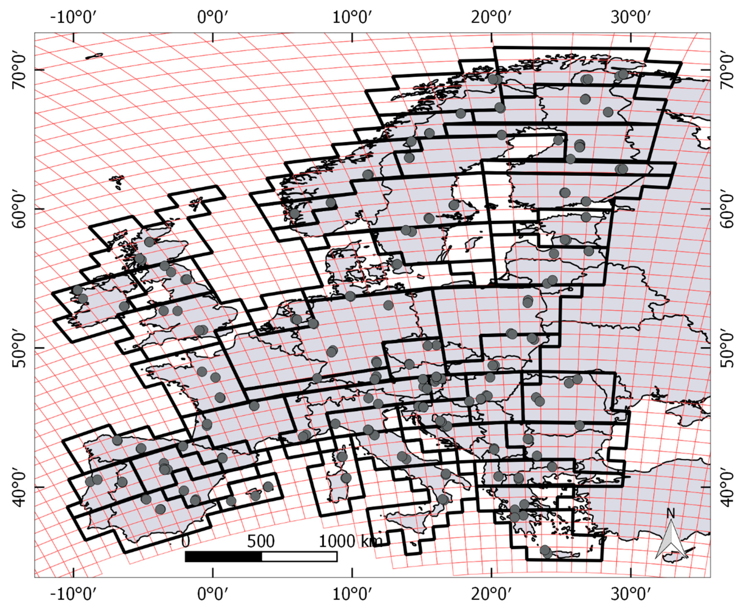
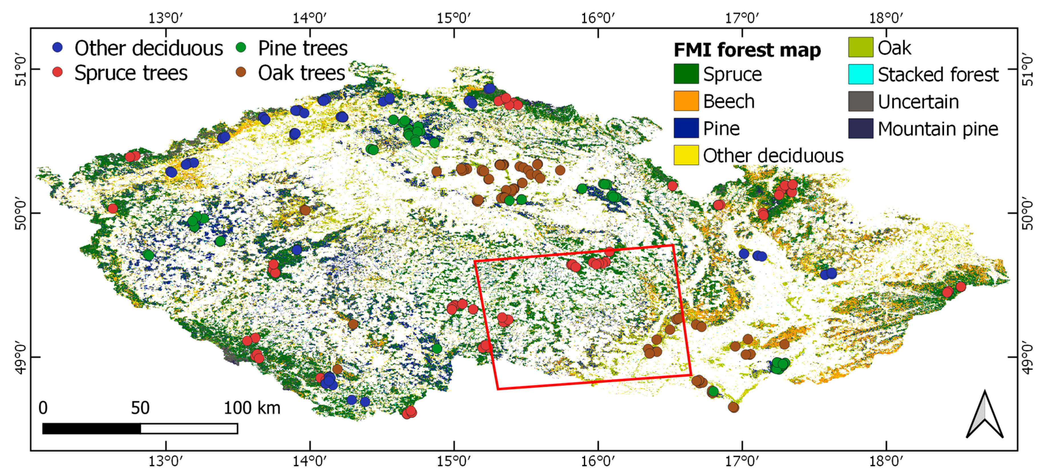
2.1.2. Validation Data

Several datasets were used for the accuracy assessment of the Sentinel-1 forest maps. These include the freely available pan-European Copernicus High Resolution Layers (HRL) 20 m Forest Type and 100 m Tree Cover Density (TCD) products [12] as well as twelve datasets from national forest inventories or universities.

The Copernicus HRL forest datasets are provided by the European Environment Agency (EEA) Global Monitoring for Environment and Security/Copernicus Initial Operations Land Service and were derived from high resolution satellite imagery from the Indian Remote Sensing-Resource SAT2 (IRS-RS2), Satellite Pour l’Observation de la Terre (SPOT) and RapidEye satellites acquired between 2011 and 2012.

The Copernicus HRL TCD dataset is defined as the vertical projection of tree crowns to a horizontal earth’s surface and represents the proportional crown coverage per pixel in percent. Minimum mapping width (MMW) of 20 m is applied, and all detectable trees are included. The forest type product specifies the dominant leaf type for each pixel (broadleaf or coniferous) and is derived from 20 m TCD product by applying a threshold of 10%, minimal mapping unit (MMU) of 0.5 ha and MMW of 20 m [12].

The overview of the available national datasets is given in Figure 1 and details are listed in

Table 1. Overview of the national datasets that were used as reference. In case of point-based datasets, the minimal mapping unit (MMU) is given in the Spatial resolution column.

Country	Dataset Provider	Data Type	Information Content	Spatial Resolution	Reference Year
Austria	Austrian Research Centre for Forests	Raster	Forest mask	1 m
Czech Republic	Forest Management Institute	Raster	Dominant tree species within pixel	10 m	2017
England, Scotland, Wales	Forestry Commission	Vector	Forest type	MMU 0.5 ha	2017
Estonia	University of Tartu	Random points	Share of conifers within forest stand	10,277 points	2017
France	Institut National de L’Information Geographique et Forestriere	Vector	Forest type	MMU 0.5 ha	2014–2019
Finland	Finnish Environment Institute	Raster	Forest type	20 m	2018
Germany	National Forest Inventory	Points	Forest type	195,630 points	2012–2017
Hungary	Nemzeti Földügyi Központ	Raster	Forest type	10 m	2020
Latvia	Latvian State Forest Research Institute Silava	Random points	Forest type	10,000 points	2019
Slovakia	Slovakian National Forest Centre	Vector	Dominant tree species within forest stand		2017
Sweden	Swedish University of Agricultural Sciences	Raster	Standing volumes of most common tree species	25 m	2010
Switzerland	National Forest Inventory	Raster	Per-pixel probability of conifers	25 m	2018

. Generally, the pre-processing of these datasets included resampling to the Equi7 grid (10 m resolution) [32] in the case of raster datasets and rasterization for the vector dataset. Due to the limited accessibility of the data in some countries, validation over Germany, Latvia and Estonia was performed point-wise using randomly selected points from respective NFIs or forest management inventories data. In cases where the dataset contained more detailed classes such as dominant tree species, the classes were adapted to coniferous (at least 65% of the coniferous tree species), broadleaved (at least 65% of broadleaf tree species) or mixed forest. The mixed forest class was used for forest/non-forest validation only. Details specific to the national datasets including the source of the data (e.g., in-situ, satellite or aerial imagery) can be found in the Appendix A.

2.2. Method

The details of the Sentinel-1 forest mapping method are described in [16] and summarized in the following subsection. The process consists of three major blocks: pre-processing, generation of SAR seasonality time series and, finally, the forest type and TCD products construction.

2.2.1. Sentinel-1 Pre-processing

The pre-processing is done using the SGRT software developed by the Technische Universität (TU) Wien [33]. The software aims at the automated processing of large volumes of SAR-based products and combines python with some external software modules. In the case of SAR pre-processing, the Sentinel Application Platform (SNAP) is used (available at https://step.esa.int/main/download/snap-download/).

The pre-processing steps include thermal noise removal, precise orbit correction, radiometric calibration to the ${\sigma }^0$ values, orthorectification using the range doppler terrain correction method [34], conversion from linear to logarithmic scale and resampling to the Equi7 Grid. The output comprises a stack of georeferenced ${\sigma }^0$ and projected local incidence angle ($\theta$) images. In [16], pre-processed images were further multi-looked to 20 m. In this study, this step was omitted, and the SAR seasonality time series and forest type products were derived at a 10 m grid which corresponds to the pixel spacing of the Sentinel-1 GRD IW dataset. In [16], forest maps were created using Sentinel-1 A data from 2015 (Sentinel-1 B was launched in April 2016), while, in the current study, both Sentinel-1 A and B data are used. As a result, approximately twice as many acquisitions are available for each pixel. Moreover, in [16] the maps were validated using Copernicus HRL forest datasets with 20 m and 100 m resolution for forest type and TCD, respectively. In this study, additional higher resolution national datasets are used for quality assessment. Therefore, we decided to omit the additional multi-looking step and derive the forest maps at the highest possible spatial resolution.

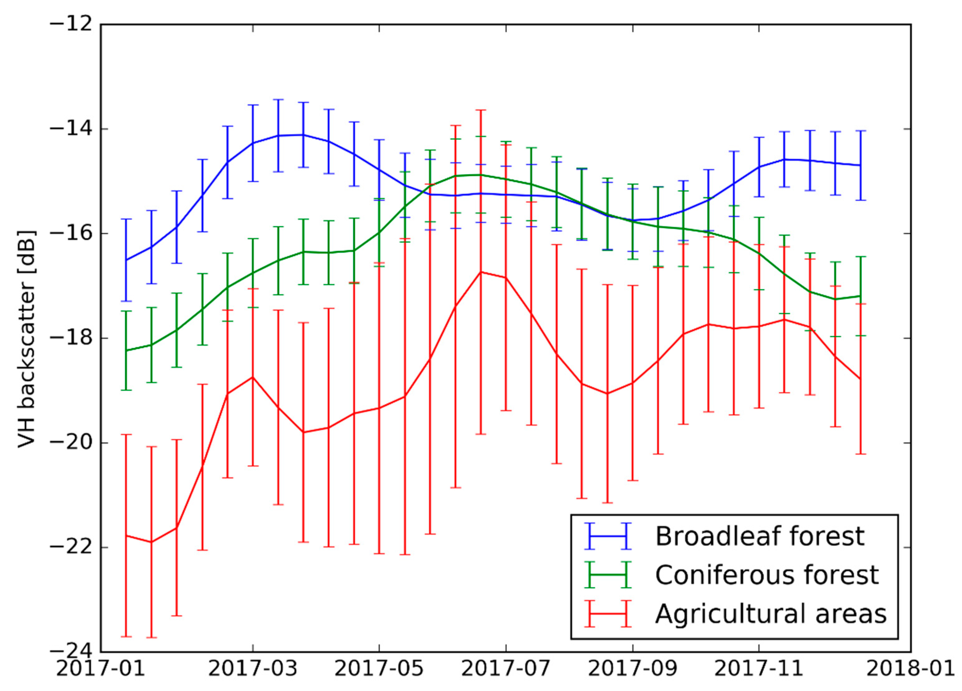
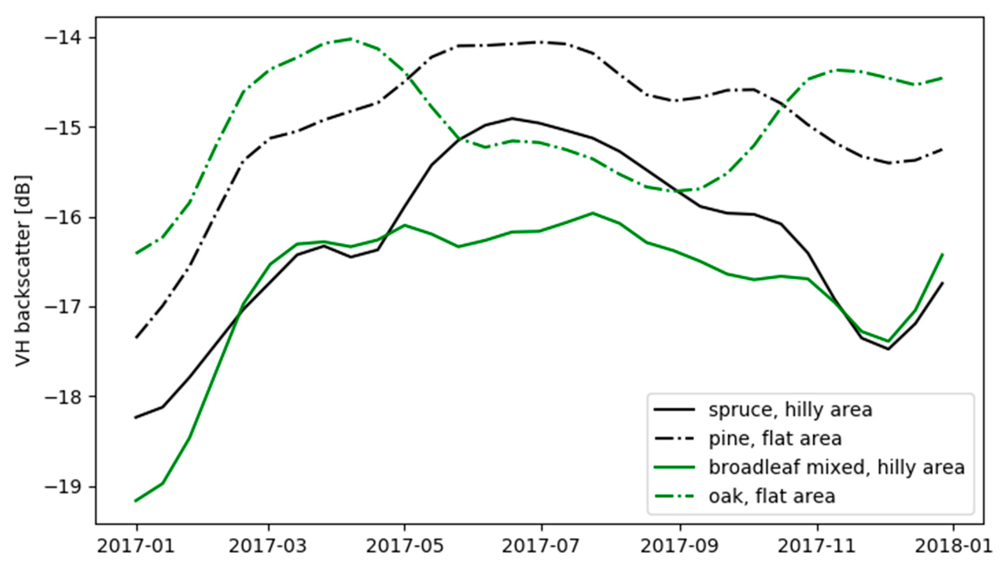
2.2.2. SAR Seasonality Time Series Computation

The SAR seasonality time series are computed from the stack of georeferenced images as temporally smoothed backscatter time series. This is done in order to reinforce the effect of the slowly varying phenological changes of vegetation and limit the noise and short-term variations caused by changing environmental conditions. To enable the combination of images acquired from different relative orbits, the backscatter images are normalized to common reference angle of 40° using the slope ($\beta$) parameter computed separately for each pixel using the linear regression between ${\sigma }^0$ and $\theta$ values. The normalisation equation reads as follows:

$${\sigma }^0\left({40}^{°}\right)={\sigma }^0\left(\theta \right)-\beta \left(\theta -\right){40}^{°}$$

(1)

Next, the mean of the normalized backscatter is computed for every 12 days (repeat orbit cycle of Sentinel-1 satellites) and the resulting time-series is again smoothed using a Gaussian temporal filter with standard deviation of 1 (corresponding to 12 days). As a result, 30 SAR seasonality values with 12-day temporal step are derived for each pixel and both polarisations. These temporal signatures show distinct behaviour over various vegetation types. Figure 2 shows an example of the temporal signatures from cross-polarised backscatter for agricultural areas (without separation of crop type, hence the large standard deviation of the signal), coniferous and broadleaf forests.

The backscatter normalisation (Equation (1)) is based on the assumption of an indirect linear relationship between backscatter (in decibel scale) and projected local incidence angle within the limited range of available incidence angles of a SAR sensor (29.1° to 46.0° in the case of Sentinel-1 and flat terrain) [22,35]. In the case of Sentinel-1, this method is, however, limited by the low number of various incidence angles in some areas, where no reliable slope value from Sentinel-1 can be derived [22]. In these areas, fixed value of $\beta$ = −0.12 is used instead, which corresponds to the average value computed over the regions, where the Sentinel-1 coverage is sufficient. Bauer-Marschalinger et al. [22] introduced an alternative approach for the $\beta$ parameter estimation over the areas of reduced Sentinel-1 coverage. This was, however, developed for lower resolution data (resampled to 500 m) and is not suitable for high resolution (10 m) data. In our study, the effect of varying local incidence angle is further reduced by temporally averaging the data within a single repeat orbit cycle—i.e., combining the measurements from all possible incidence angles into a single value—which is why we consider the simplified slope computation sufficient for this application. Furthermore, the $\beta$ parameter varies with vegetation growth [36], yet it was assumed to be temporally stable, as a single year of Sentinel-1 data is not sufficient to compute its seasonal variation.

2.2.3. Construction of Forest Maps

The forest classification algorithm exploits the differences between the temporal signatures of various vegetation types (Figure 2). Signature prototypes are defined for coniferous and broadleaf forest classes. Due to the large variability of forests and their temporal signatures across Europe, the continent was stratified into smaller regions, and, for each region, four signature prototypes were selected and computed. The prototypes are computed as described in the previous chapter using averaged backscatter values over 300 m × 300 m large forested areas (30 × 30 pixels) and are selected to represent both coniferous and broadleaved forest types in each region—typically two prototypes for each class. The regions were selected manually so that they contain areas with similar biomes, forest types and terrain variations using the digital terrain model and the map of habitat suitability of European forest categories [37]. The borders of the regions correspond to the borders of the Equi7 grid tiles. The selection of the signature prototypes location was supported by reference datasets that included Copernicus HRL maps, national forest datasets or orthophotos (if available) as well as average Sentinel-1 backscatter for 2017 to exclude areas with apparent terrain effects or clear cuts. The regions (bold black lines) and reference points (grey dots) are presented in Figure 3. Figure 4 shows an example prototype time series in an area covering central Europe. Note that the difference between the pure stands of a particular tree species might be larger than that between the coniferous and broadleaf forest type, which is why it is essential to select the reference points accordingly in order to be representative for the most common tree species in each area.

The similarity measures—Root Mean Square Difference (RMSD) and Pearson correlation coefficient (r)—between the prototype signatures and the respective temporal signature of each image pixel are used for the classification. In the first step, forest/non-forest classification is performed using thresholds that are fixed for entire Europe. Threshold values are 1.5 dB and 2.0 dB for VH and VV polarisation RMSD, respectively, and 0.4 for VH polarisation r. These values were empirically set in [16] as the best fitting for three test sites from Austria to northern Sweden. Each pixel that falls within the thresholds with similarity measures computed for any of the prototype time series is classified as forest; the rest is classified as non-forest. With method, no signature prototypes need to be defined for land cover types other than forests. The forest type (coniferous, broadleaved) is then assigned to each forested pixel according to the lowest RMSD value in VH polarisation. The VH polarisation was selected for the forest type classification due to higher sensitivity of the cross-polarised backscatter to the forest structure [23,38]. For the final forest type product, the MMU of 0.5 ha is applied and the 100 m TCD product is computed as the fraction of the 10 m pixels within each 100 m × 100 m target area that were classified as forests (prior to MMU application).

2.2.4. Validation

The accuracy assessment of the Sentinel-1 forest maps was performed in two steps. First, validation metrics between Copernicus HRL datasets and Sentinel-1 forest maps were computed on pan-European level as well as for each 100 km × 100 km Equi7 tile. Second, both Sentinel-1 and Copernicus HRL forest maps were compared to the national forest datasets. The computed validation metrics included overall accuracy (OA, Equation (2)), producer’s (PA), and user’s (UA) accuracies (Equations (3) and (4), respectively).

$$OA=\frac{T}{N}$$

(2)

$$P{A}_{cl}=\frac{T{R}_{cl}}{N{R}_{cl}}$$

(3)

$$U{A}_{cl}=\frac{T{C}_{cl}}{N{C}_{cl}}$$

(4)

In these equations, T stands for number of correctly classified pixels, N for number of all pixels used for validation, TR_cl for number of correctly classified reference pixels of respective class cl, NR_cl for number of all reference pixels of respective class cl, TC_cl for number of all correctly classified pixels within respective class cl and NC_cl for number of all pixels classified into respective class cl. The accuracies were computed for forest/non-forest classification as well as for forest type classification (broadleaved or coniferous forest type computed for all pixels classified as forests in both datasets). Furthermore, Pearson correlation coefficient and bias were computed between the TCD products.

The national datasets varied in format and provided information. In the case of raster and rasterised datasets, the statistics were computed for all pixels, while in the case of pointwise comparison, the point information was compared to the corresponding pixel. In the case of national datasets over Estonia and Latvia, only forest type accuracy was computed, as the respective forest inventories do not contain all forested land. Moreover, the forest map of Lower Austria allowed only forest/non-forest validation due to the lack of forest type information.

2.2.5. Sensitivity Analysis

One of the main challenges of the introduced approach is the susceptibility of the results to the selection of the signature prototypes used for the forest classification. To quantify this effect, we performed a sensitivity test over a single Equi7 grid tile (100 km × 100 km) located in the Czech Republic. A total of 80 sets of reference points were selected for the forest classes with dominant tree types spruce, pine, oak and other deciduous forest. The points were selected using the Czech Forest Management Institute forest map. Forest type and TCD maps were computed for each set of reference points and the results were validated against the Copernicus HRL forest maps. The overview of the test site and the locations of the selected reference points are shown in Figure 5.

3. Results

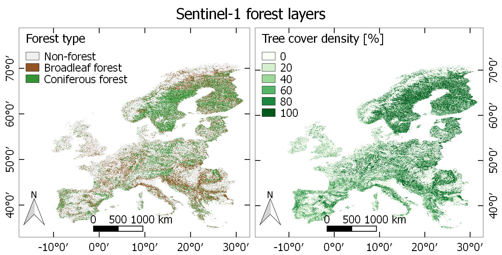
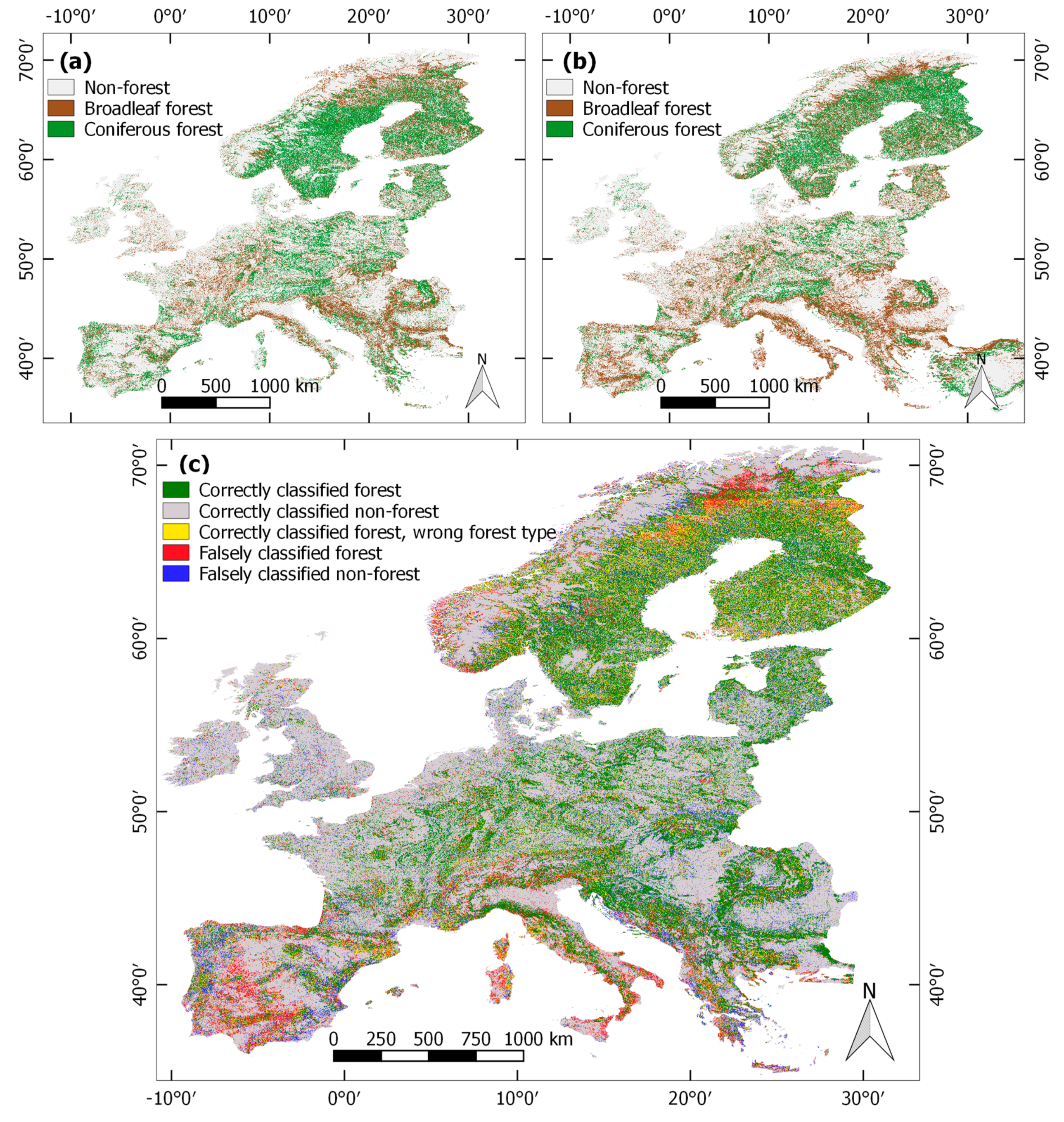
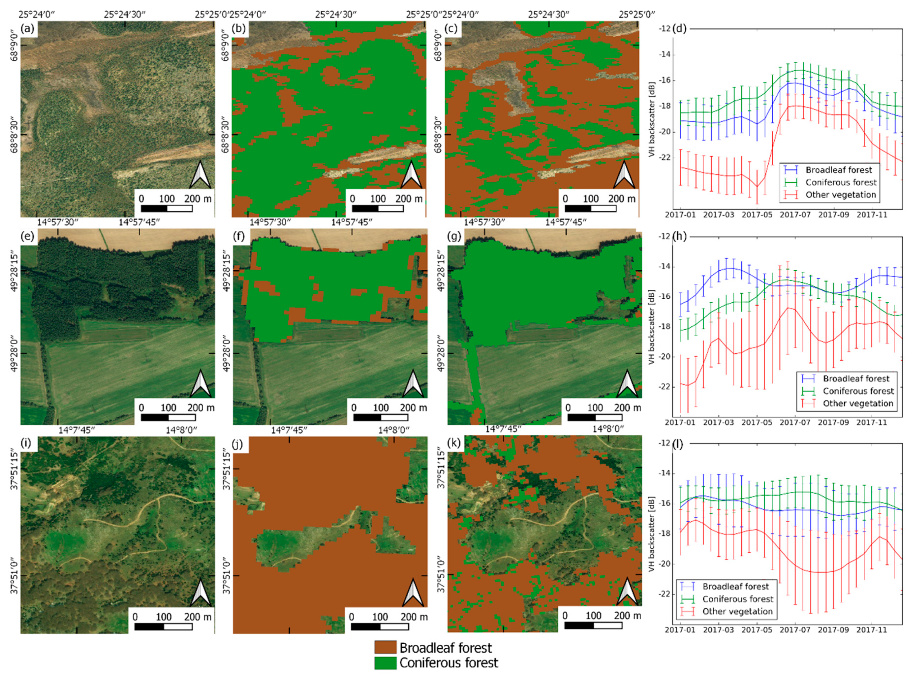
3.1. Forest Area and Forest Type

The accuracy of the Sentinel-1 forest type map was assessed both on the European level using the Copernicus HRL forest type products as well as on the national level using the various national datasets. The forest type maps from Sentinel-1 and Copernicus HRL over the European Continent are shown in Figure 6, while Figure 7 and Figure 8 present the forest type map for Czech Republic and Sicily, respectively. The Figure 6, Figure 7 and Figure 8 also include a difference image highlighting the discrepancies between the two products in red (pixels classified as forest in the Copernicus HRL forest type dataset and as non-forest in the Sentinel-1 forest type dataset), blue (pixels classified as non-forest in the Copernicus HRL forest type dataset and as non-forest in the Sentinel-1 forest type map) and light green (pixels classified as forests in both datasets but assigned different forest types).

3.1.1. Copernicus HRL Dataset

Table 2. Accuracy of the Sentinel-1 forest/non-forest and forest type map when compared to the Copernicus High Resolution Layers forest type dataset. The accuracies are summarized for the whole of Europe.

	Forest/non-Forest	Forest Type
Overall accuracy	0.86	0.73
Producers’ accuracy forest/broadleaf	0.83	0.81
Users’ accuracy forest/broadleaf	0.81	0.68
Producers’ accuracy non-forest/coniferous	0.88	0.66
Users’ accuracy non-forest/coniferous	0.89	0.79

shows the accuracies for forest/non-forest and forest type classification computed for the entire study area. The overall accuracy is 86.1% for forest area and 73.2% for forest type, respectively. Since these accuracies strongly vary across the continent, spatial maps showing the overall accuracies for both forest/non-forest classification and forest types are presented in Figure 9. The numbers were specified for each 100 km × 100 km area which represents one Equi7 tile.

Typical results over flatland and hilly areas with the main differences between the Sentinel-1 map and the reference datasets are highlighted in Figure 10. The Sentinel-1 forest type product generally overestimates the forest area in flatlands. In the case of small villages or agricultural areas, some parts are often classified as forests. This is due to large number of trees in gardens or hedgerows between fields or among roads. In addition, vineyards or orchards are common areas of disagreement between the Sentinel-1 forest type map and reference datasets. Vineyards are commonly falsely classified as coniferous forests in Sentinel-1 forest type product while apple orchards are assigned to non-forests class in Sentinel-1 forest type map, but they are often classified as broadleaved forests in the Copernicus forest type product. Lastly, in areas with large terrain variations, false gaps in forests caused by terrain distortions in SAR data can be observed.

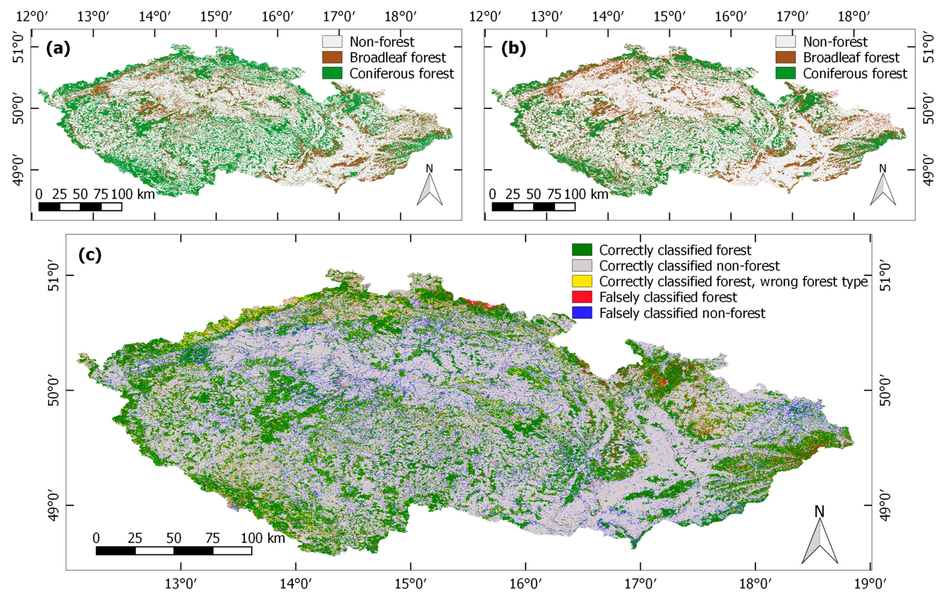
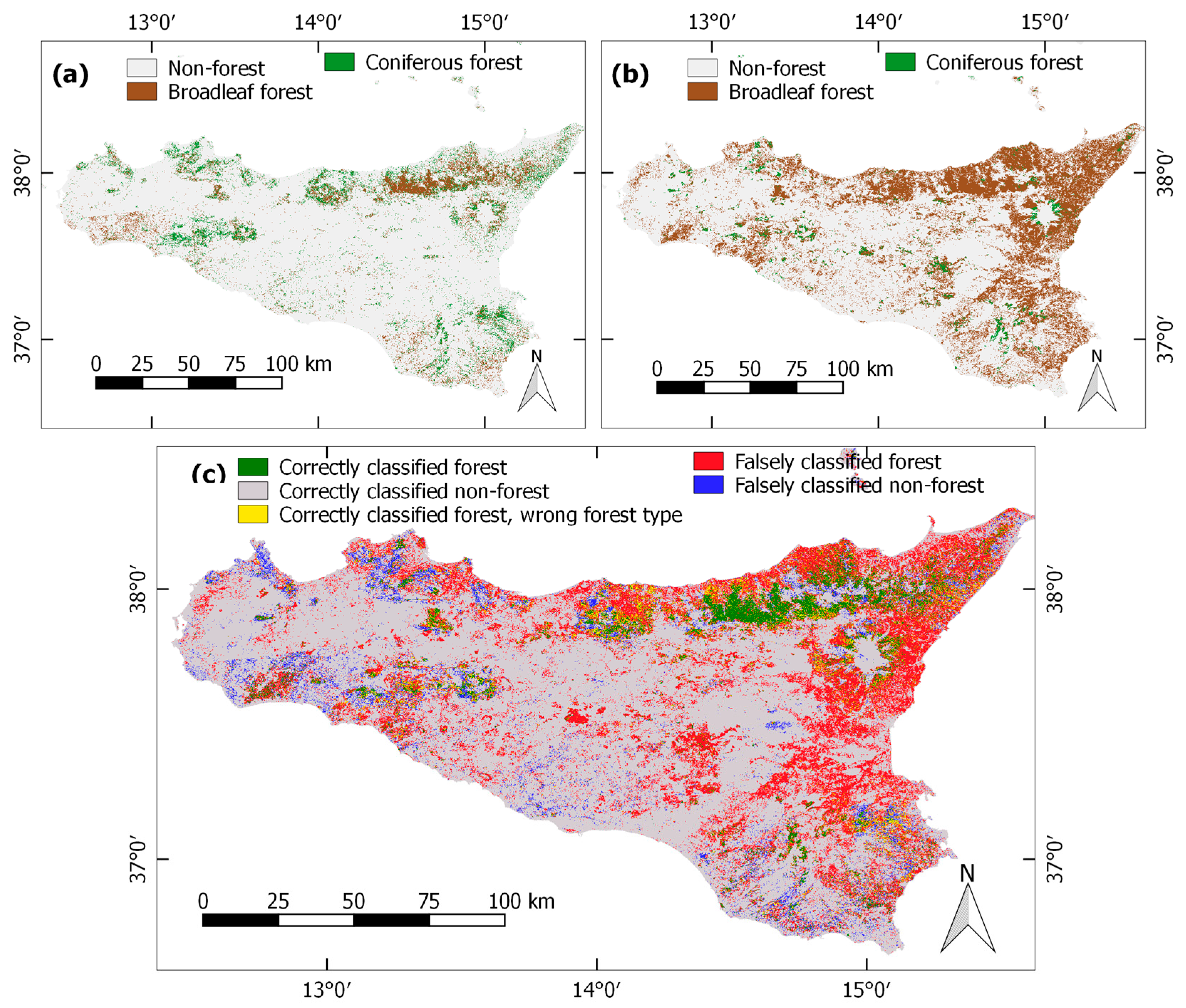
3.1.2. National Datasets

The Copernicus HRL dataset is based on optical satellite imagery, and, according to the validation report, the users’ and producers’ accuracies vary between 83% and 93% for forest/non forest classification, and between 17% and 98% for forest type, with the lowest accuracies in the boreal and alpine regions. As the highest disagreement between our product and the Copernicus HRL forest type map can be found in these regions, alternative sources of data are needed to better assess the accuracy of both products. For this reason, we compared both maps to different national datasets.

Table 3. Results of the accuracy assessment using the national datasets for the forest/non-forest classification. The following statistics are listed: overall accuracy (OA), producers’ accuracy (PA) and users’ accuracy (UA).

	Sentinel 1 vs. Reference					Copernicus vs. Reference
		Forest		Non-Forest			Forest		Non-Forest
	OA	PA	UA	PA	UA	OA	PA	UA	PA	UA
Austria	0.91	0.92	0.87	0.90	0.95	0.93	0.93	0.90	0.93	0.95
Czech Republic	0.90	0.94	0.79	0.87	0.97	0.95	0.93	0.91	0.95	0.96
England, Scotland, Wales	0.91	0.74	0.50	0.93	0.97	0.93	0.80	0.56	0.94	0.97
France	0.90	0.83	0.84	0.93	0.92	0.92	0.89	0.87	0.94	0.95
Finland	0.88	0.92	0.88	0.82	0.88	0.87	0.94	0.86	0.77	0.89
Germany	0.93	0.95	0.83	0.92	0.98
Hungary	0.88	0.88	0.66	0.88	0.97	0.92	0.85	0.79	0.94	0.96
Slovakia	0.82	0.93	0.72	0.75	0.94	0.88	0.93	0.81	0.85	0.95
Sweden	0.82	0.88	0.83	0.73	0.81	0.82	0.88	0.83	0.73	0.81
Switzerland	0.87	0.78	0.76	0.91	0.91	0.88	0.94	0.72	0.86	0.97

shows the respective accuracies for forest/non-forest classification and

Table 4. Results of the accuracy assessment using the national datasets for the forest type classification. The following statistics are listed: overall accuracy (OA), producers’ accuracy (PA) and users’ accuracy (UA).

	Sentinel 1 vs. Reference					Copernicus vs. Reference
		Broadleaf		Coniferous			Broadleaf		Coniferous
	OA	PA	UA	PA	UA	OA	PA	UA	PA	UA
Czech Republic	0.84	0.72	0.88	0.93	0.81	0.89	0.95	0.81	0.84	0.96
England, Scotland, Wales	0.74	0.95	0.64	0.56	0.93	0.80	0.95	0.68	0.69	0.95
Estonia	0.87	0.77	0.97	0.97	0.79
France	0.84	0.87	0.92	0.75	0.62	0.91	0.96	0.93	0.77	0.86
Finland	0.71	0.75	0.14	0.71	0.98	0.88	0.93	0.31	0.88	0.99
Germany	0.91	0.94	0.89	0.87	0.93
Hungary	0.80	0.81	0.98	0.69	0.15	0.97	0.98	0.99	0.76	0.71
Latvia	0.85	0.68	0.90	0.70	0.90
Slovakia	0.90	0.93	0.92	0.83	0.86	0.88	0.97	0.87	0.72	0.93
Sweden	0.82	0.45	0.16	0.84	0.96	0.79	0.87	0.21	0.79	0.99
Switzerland	0.82	0.78	0.83	0.85	0.80	0.86	0.83	0.87	0.89	0.86

for the forest type, respectively. The mountainous regions are well represented in Switzerland and Slovakia, while the boreal regions are covered by datasets from Finland and Sweden.

For forest/non-forest classification, the comparison with most of the national datasets reveals overall accuracies of around 90%. The highest correspondence was obtained for Germany with an accuracy of 93%, and the lowest overall accuracies of 82% were obtained for Slovakia and Sweden. For Switzerland, the most mountainous country in Europe, a high overall accuracy of 87% was obtained. For Finland, that is also predominantly covered by boreal forests, an accuracy of 88% was obtained.

Generally, the correspondence between the Sentinel-1 forest type map and national datasets is slightly lower than between the Copernicus HRL forest type product and national datasets. The highest difference can be observed in the case of the Czech Republic, where the overall accuracies of 95% and 90% were obtained in the case of Copernicus and our product, respectively. On the other hand, in Finland, the Sentinel-1 dataset shows slightly higher overall accuracy than the Copernicus HRL dataset (88% when compared to 87%). In most of the other cases, the difference is around 2%. Except Sweden, the Copernicus HRL dataset shows high accuracies for forest/non-forest mapping, which confirms that it may be used as a reliable reference dataset.

For the forest type classification, the variability between the results for various national datasets is much higher than in the case of the forest/non-forest mapping. For the Sentinel-1 forest type product, remarkably high accuracies can be observed over Germany (91%), Slovakia (90%) or Estonia (87%). On the other hand, problems can be observed in Sweden and Finland, where the overall accuracies are 82% and 71%, respectively, and the users’ accuracies for broadleaf forests are very low (16% and 14%, respectively). The same effect can be observed for the Copernicus HRL dataset, where the users’ accuracies of broadleaf forests are 21% and 31% for Sweden and Finland, respectively. In addition, England, Scotland and Wales show lower accuracies for both datasets—74% in the case of Sentinel-1 and 80% in the case of the Copernicus forest type product. In both cases, the lower users’ accuracies of broadleaf forests and producers’ accuracies of coniferous forests indicate that the broadleaf forests tend to be overestimated, while the coniferous tend to be underestimated in both Sentinel-1 and Copernicus HRL forest type maps.

Moreover, the differences between the accuracies of the Copernicus HRL and Sentinel-1 forest type datasets are much higher, reaching up to 17% in the case of Finland and Hungary. In the case of Hungary, this is caused by strong overestimation of coniferous forests in the case of the Sentinel-1 forest type map (users’ accuracy of only 15% for coniferous forests and overall accuracy of 80%). On the other hand, in the case of Slovakia and Sweden, Sentinel-1 shows slightly higher overall accuracies than the Copernicus HRL dataset. Generally, overall accuracies in the case of the Sentinel-1 forest type map vary between 71% for Finland and 91% for Germany, while, for Copernicus, they vary between 79% for Sweden and 97% in Hungary.

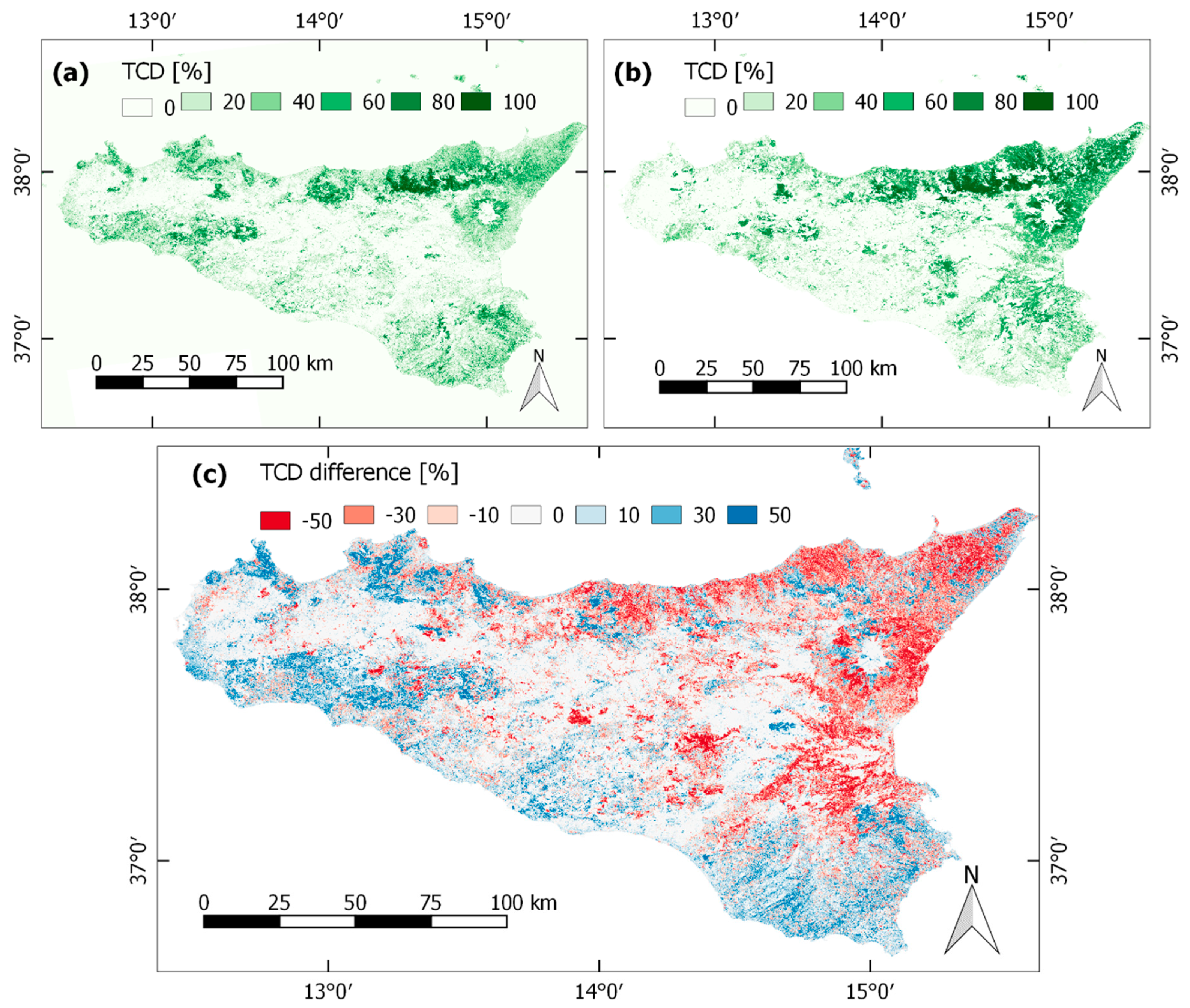
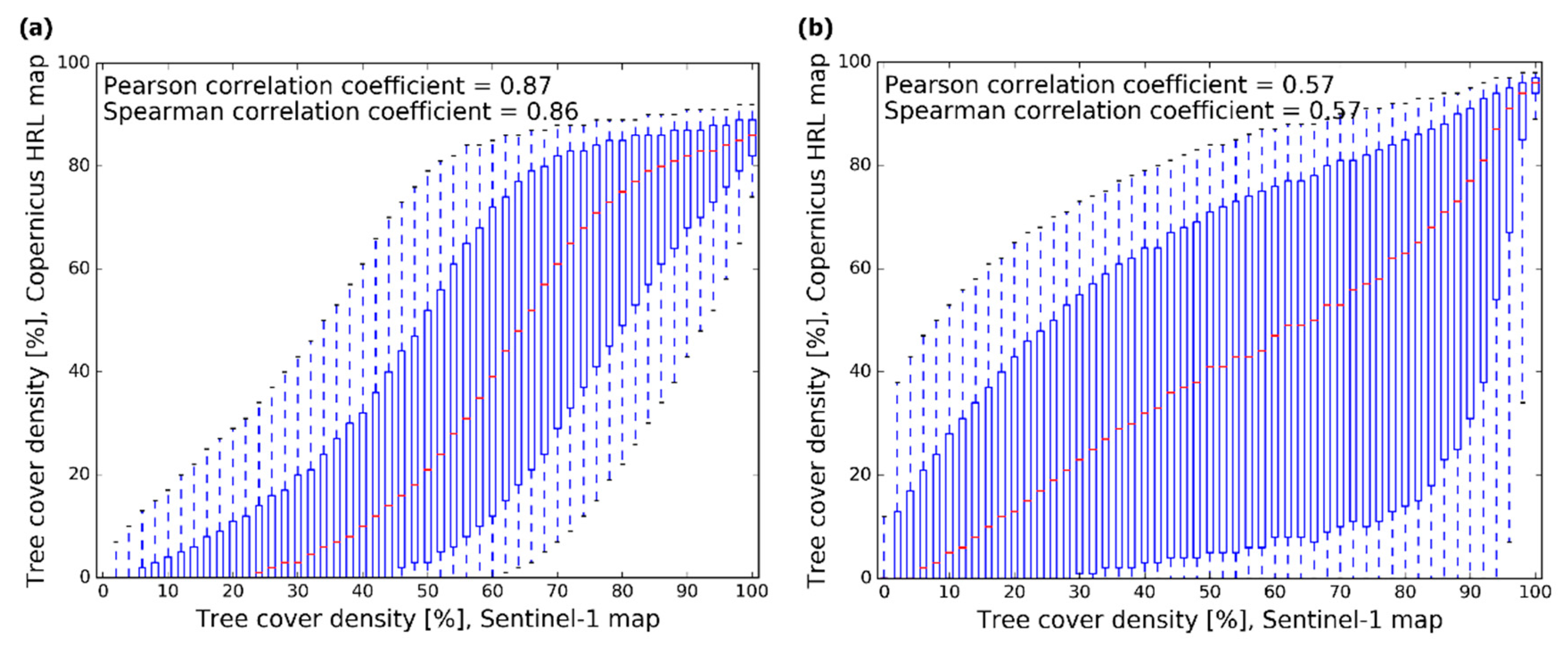
3.2. Tree Cover Density

The TCD map was validated using the Copernicus TCD dataset only. Both maps, including the difference map as well as the spatial distribution of the r value between the two, are presented at Figure 11 and Figure 12, respectively. The r value computed for entire Europe is 0.83 and the bias corresponds to 9.8%, showing that the Sentinel-1 based map overestimates the tree cover density values when compared to the Copernicus product. This is especially visible in the northern part of Europe. While the TCD values in Sweden and Finland often reach 100% for the Sentinel-1 map, they range between 60% and 80% in the case of the Copernicus HRL dataset. Over central Europe, the TCD patterns correspond well and the differences increase towards the south of Europe again.

To get a spatial overview, r was also computed for each Equi7 tile (100 km × 100 km area) separately. The spatial distribution (Figure 12) shows strong correspondence with values between 0.85 and 0.95 over large parts of central, eastern, and northern Europe. Lower accuracies (r between 0.65 and 0.85) can be observed over Alpine areas, southern Europe, the United Kingdom, Norway, and part of Sweden. Values below 0.65 are located mainly in southern Italy, southern Spain, Portugal, the islands of Corsica and Sardinia, and coastal areas of Greece, Albania, Croatia, and Norway. These areas typically have uneven topography and steep slopes.

An example of results for the Czech Republic (r = 0.90) and Sicily (r = 0.53) are presented in Figure 13 and Figure 14, respectively. Figure 15 shows boxplot distribution of TCD values for these two regions.

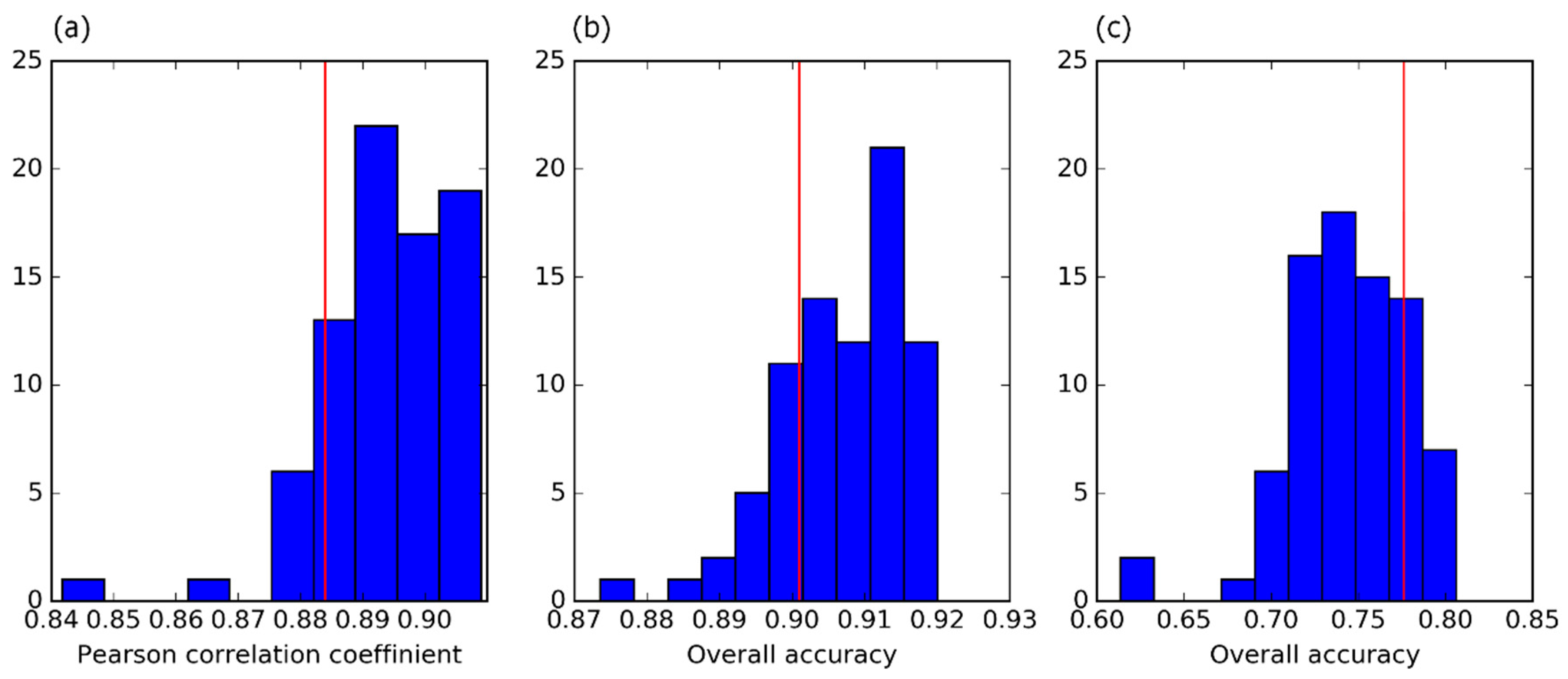
3.3. Sensitivity Analysis

Within the sensitivity analysis, 80 forest type and TCD maps were derived for a single Equi7 tile and compared to the Copernicus HRL datasets. The results are presented in Figure 16 with the red line indicating the value of the original set of signature prototypes. In the case of the forest type map, overall accuracies range between 87.4% and 92.0% for forest/non forest, and between 60.3% and 80.6% for forest type classification. The values of the original set of signature prototypes are 90.1% and 77.6% for the forest/non-forest and forest type classification, respectively. In the case of the TCD map, r ranges between 0.84 and 0.91, with 0.88 for the original set of signature prototypes.

4. Discussion

4.1. Performance of the Sentinel-1 Based Forest Maps

The accuracy assessment revealed that the approach is well suited for temperate and hemi-boreal forests; however, its ability to detect forested areas or classify forest type decreases in areas with lower forest density such as Mediterranean forests or areas in northern Sweden and Norway. Sparser tree coverage in these areas causes lower differences between the temporal signatures of different vegetation types (Figure 17). The high density of temperate forests enables the separation between forest/non-forest as well as forest type classification, while in Mediterranean forests, differentiation between the three classes is often not possible. High omission errors are to be expected, especially in areas with very sparse tree coverage. While in boreal forests, separation between forest and non-forest is feasible, the seasonal drop in temporal signature of broadleaf tree species is no longer visible and it is, therefore, difficult to distinguish between the two forest types (Figure 17). The same applies in high altitudes in montane forests where the approach is further limited by the topographic distortions in SAR signal. A more appropriate approach for terrain correction, such as using the terrain flattened gamma [39] might improve the results over mountainous areas. Nevertheless, results for Finland (overall accuracy of 88% for forest/non-forest mapping and 71% for forest type classification) or Switzerland (87% for forest/non forest mapping and 82% for forest type classification) show high potential of Sentinel-1 for forest mapping even in these challenging environments.

Forest area mapping for relatively small areas based on Sentinel-1 data was recently addressed in several studies. Overall accuracies of 94% were found over study area in North-East China [31], 92% over study area in Lower Austria [30], and balanced accuracies between 80% and 93% were reported for six sites distributed worldwide [14]. Forest type (coniferous/broadleaf) classification using Sentinel-1 was tested in two test sites in Switzerland [15] with overall accuracy of 86%. Due to the limited size of the study sites located in Europe, no direct comparison can be made with the presented results. To the best of our knowledge, the only continental or global scale forest/non-forest map based on the SAR backscatter data is derived yearly by the Japan Aerospace Exploration Agency (JAXA) from Advanced Land Observing Satellite (ALOS) Phased Arrayed L-band SAR (PALSAR) data [10]. Overall accuracy of the global ALOS PALSAR map was estimated at between 85% and 95% depending on the reference data used [10]. The overall accuracy of the presented Sentinel-1 based map ranges from 86% when compared to Copernicus HRL data to 90% when compared to the national datasets.

4.2. Selection of the Reference Time Series

One of the main challenges of the introduced approach is the susceptibility of the results to the choice of the temporal signature prototypes used for the forest classification. The selection of their location represents the only part that cannot be automated and requires not only manual interaction, but also local knowledge of the area or reliable reference data. We aimed to quantify the effect of the reference points selection by running the model repeatedly using different sets of signature prototypes. Our results show that, while the forest/non-forest and TCD accuracy is rather stable (overall accuracy between 87.4% and 92.0%), the forest type accuracy shows higher variation among the different sets of reference points (overall accuracy between 61.3% and 80.6%). Inspection of the Sentinel-1 data revealed that lowest accuracies for the forest type map are related to the selection of the spruce forest reference point located in areas with visible terrain effects. However, within the sensitivity test, the main tree species were known, and a reliable reference dataset was available to support the signature prototypes selection. Accuracy might vary even more strongly in cases where the most common tree species are not captured by the signature prototypes. In the case of the full-European study, it was not feasible to select all reference points accordingly, so that they would represent the most common forest species in the area. In some areas, better selection supported with the knowledge of local conditions might improve the result substantially. However, once the reference points are selected, the approach can rather easily be applied automatically, creating yearly forest maps with no further need of manual interaction, which enables change detection and regular updates of forestry data. As such, it might complement the well-established methods using optical remote sensing data.

4.3. Variability of National Reference Datasets

Relatively high variability of results between the national datasets and both the Sentinel-1 and Copernicus HRL datasets is caused by the large variability of the data sources, formats, resolutions as well as different definitions used for the coniferous and broadleaf classes for the validation. The reference data itself are often, at least partially, based on the remote sensing data and include errors as well. Furthermore, their accuracies were mostly unknown. Temporal gaps between the datasets also add to the uncertainties, especially in the case of the Swedish map, which was created in 2010. Lastly, also the differences in forest definitions play an important role in the validation results. The Sentinel-1 map applies the MMU of 0.5 ha, but apart from the definition of the minimal area, no further rules are applied to identify the pixel as forest. For this reason, areas with high density of woodland, such as hedgerows or gardening areas, are commonly misclassified as forest. On the other hand, some of the national datasets include the unstocked forest land in the forest class, which leads to further discrepancies between the datasets.

4.4. Areas of Further Research

The radiometric terrain flattening [39] is expected to increase the applicability of Sentinel-1 in mountainous areas and can, therefore, improve the results over complex terrain. In the present study, this approach was not used due to large demand on processing resources due to the extensive test area. Testing and validating the approach using the terrain flattened gamma backscatter is one of the foreseen further steps. In addition, many areas were still validated using the Copernicus HRL data only, so including more national datasets—also for the tree cover density map—would provide a better overview of the quality of the Sentinel-1 forest products.

5. Conclusions

In this study, the first Europe-wide forest maps were introduced based on Sentinel-1 data only. These include a 10 m forest type map and a 100 m tree cover density map. The comprehensive validation included comparison with Copernicus HRL forest datasets and a variety of national datasets. The validation using national datasets showed that the Sentinel-1 forest maps have comparable accuracy with Copernicus HRL forest datasets, with average overall accuracies of 88.2% and 82.7% for Sentinel-1 and 90% and 87.2% for Copernicus HRL for forest/non-forest and forest type maps, respectively. The main advantage of the Sentinel-1 maps is that once the model, including reference points estimation, is established, yearly maps can be derived in a fully automated way. The spatial comparison with the Copernicus HRL dataset showed that the method works best in temperate broadleaf forest biomes, while the accuracy decreases in Mediterranean, boreal and montane forests.

References

1. Nabuurs, G.; Päivinen, R.; Sikkema, R.; Mohren, G. The role of European forests in the global carbon cycle—A review. Biomass Bioenergy 1997, 13, 345–358. [Google Scholar] [CrossRef]
2. Grace, J. Understanding and managing the global carbon cycle. J. Ecol. 2004, 92, 189–202. [Google Scholar] [CrossRef]
3. Pimentel, D.; Kounang, N. Ecology of soil erosion in ecosystems. Ecosystems 1998, 1, 416–426. [Google Scholar] [CrossRef]
4. Calder, I.; Hofer, T.; Vermont, S.; Warren, P. Towards a new understanding of forests and water. UNASYLVA-FAO- 2008, 229, 3. [Google Scholar]
5. Ernst, C.; Gullick, R.; Nixon, K. Conserving forests to protect water. Opflow 2004, 30, 1–7. [Google Scholar] [CrossRef]
6. Borre, J.V.; Paelinckx, D.; Mücher, C.A.; Kooistra, L.; Haest, B.; De Blust, G.; Schmidt, A.M. Integrating remote sensing in Natura 2000 habitat monitoring: Prospects on the way forward. J. Nat. Conserv. 2011, 19, 116–125. [Google Scholar] [CrossRef]
7. Barrett, F.; McRoberts, R.E.; Tomppo, E.; Cienciala, E.; Waser, L.T. A questionnaire-based review of the operational use of remotely sensed data by national forest inventories. Remote Sens. Environ. 2016, 174, 279–289. [Google Scholar] [CrossRef]
8. White, J.C.; Coops, N.C.; Wulder, M.A.; Vastaranta, M.; Hilker, T.; Tompalski, P. Remote Sensing Technologies for Enhancing Forest Inventories: A Review. Can. J. Remote Sens. 2016, 42, 619–641. [Google Scholar] [CrossRef] [Green Version]
9. Kangas, A.; Astrup, R.; Breidenbach, J.; Fridman, J.; Gobakken, T.; Korhonen, K.T.; Maltamo, M.; Nilsson, M.; Nord-Larsen, T.; Næsset, E.; et al. Remote sensing and forest inventories in Nordic countries–roadmap for the future. Scand. J. For. Res. 2018, 33, 397–412. [Google Scholar] [CrossRef] [Green Version]
10. Shimada, M.; Itoh, T.; Motooka, T.; Watanabe, M.; Shiraishi, T.; Thapa, R.; Lucas, R. New global forest/non-forest maps from ALOS PALSAR data (2007–2010). Remote Sens. Environ. 2014, 155, 13–31. [Google Scholar] [CrossRef]
11. Hansen, M.C.; Potapov, P.V.; Moore, R.; Hancher, M.; Turubanova, S.A.; Tyukavina, A.; Thau, D.; Stehman, S.V.; Goetz, S.J.; Loveland, T.R.; et al. High-Resolution Global Maps of 21st-Century Forest Cover Change. Science 2013, 342, 850–853. [Google Scholar] [CrossRef] [Green Version]
12. Langanke, T.; Büttner, G.; Dufourmont, H.; Iasillo, D.; Probeck, M.; Rosengren, M.; Sousa, A.; Strobl, P.; Weichselbaum, J. GIO land (GMES/Copernicus initial operations land) High Resolution Layers (HRLs)–summary of product specifications. In European Environment Agency Copernicus Report; European Environmental Agency: Copenhagen, Denmark, 2013; Available online: https://land.copernicus.eu/user-corner/technical-library/gio-land-high-resolution-layers-hrls-2013-summary-of-product-specifications (accessed on 18 January 2021).
13. Lang, M.; Kaha, M.; Laarmann, D.; Sims, A. Construction of tree species composition map of Estonia using multispectral satellite images, soil map and a random forest algorithm. For. Stud. 2018, 68, 5–24. [Google Scholar] [CrossRef] [Green Version]
14. Hansen, J.N.; Mitchard, E.T.; King, S. Assessing Forest/Non-Forest Separability Using Sentinel-1 C-Band Synthetic Aperture Radar. Remote Sens. 2020, 12, 1899. [Google Scholar] [CrossRef]
15. Rüetschi, M.; Schaepman, M.E.; Small, D. Using multitemporal sentinel-1 c-band backscatter to monitor phenology and classify deciduous and coniferous forests in northern switzerland. Remote Sens. 2018, 10, 55. [Google Scholar] [CrossRef] [Green Version]
16. Dostálová, A.; Wagner, W.; Milenković, M.; Hollaus, M. Annual seasonality in Sentinel-1 signal for forest mapping and forest type classification. Int. J. Remote Sens. 2018, 39, 7738–7760. [Google Scholar] [CrossRef]
17. Imhoff, M.L. Radar backscatter/biomass saturation: Observations and implications for global biomass assessment. In Proceedings of the IGARSS’93-IEEE International Geoscience and Remote Sensing Symposium, Tokyo, Japan, 18–21 August 1993; pp. 43–45. [Google Scholar]
18. Lucas, R.; Armston, J.; Fairfax, R.; Fensham, R.; Accad, A.; Carreiras, J.; Kelley, J.; Bunting, P.; Clewley, D.; Bray, S. An evaluation of the ALOS PALSAR L-band backscatter—Above ground biomass relationship Queensland, Australia: Impacts of surface moisture condition and vegetation structure. IEEE J. Sel. Top. Appl. Earth Obs. Remote Sens. 2010, 3, 576–593. [Google Scholar] [CrossRef]
19. Ranson, K.J.; Sun, G. Effects of environmental conditions on boreal forest classification and biomass estimates with SAR. IEEE Trans. Geosci. Remote Sens. 2000, 38, 1242–1252. [Google Scholar] [CrossRef]
20. Santoro, M.; Beer, C.; Cartus, O.; Schmullius, C.; Shvidenko, A.; McCallum, I.; Wegmüller, U.; Wiesmann, A. Retrieval of growing stock volume in boreal forest using hyper-temporal series of Envisat ASAR ScanSAR backscatter measurements. Remote Sens. Environ. 2011, 115, 490–507. [Google Scholar] [CrossRef]
21. Torres, R.; Snoeij, P.; Geudtner, D.; Bibby, D.; Davidson, M.; Attema, E.; Potin, P.; Rommen, B.; Floury, N.; Brown, M.; et al. GMES Sentinel-1 mission. Remote Sens. Environ. 2012, 120, 9–24. [Google Scholar] [CrossRef]
22. Bauer-Marschallinger, B.; Freeman, V.; Cao, S.; Paulik, C.; Schaufler, S.; Stachl, T.; Modanesi, S.; Massari, C.; Ciabatta, L.; Brocca, L.; et al. Toward Global Soil Moisture Monitoring With Sentinel-1: Harnessing Assets and Overcoming Obstacles. IEEE Trans. Geosci. Remote Sens. 2019, 57, 520–539. [Google Scholar] [CrossRef]
23. Patel, P.; Srivastava, H.S.; Panigrahy, S.; Parihar, J.S. Comparative evaluation of the sensitivity of multi-polarized multi-frequency SAR backscatter to plant density. Int. J. Remote Sens. 2006, 27, 293–305. [Google Scholar] [CrossRef]
24. Frison, P.-L.; Fruneau, B.; Kmiha, S.; Soudani, K.; Dufrêne, E.; Le Toan, T.; Koleck, T.; Villard, L.; Mougin, E.; Rudant, J.-P. Potential of Sentinel-1 data for monitoring temperate mixed forest phenology. Remote Sens. 2018, 10, 2049. [Google Scholar] [CrossRef] [Green Version]
25. Srivastava, P.K.; O’Neill, P.; Cosh, M.; Lang, R.; Joseph, A. Evaluation of radar vegetation indices for vegetation water content estimation using data from a ground-based SMAP simulator. In Proceedings of the 2015 IEEE International Geoscience and Remote Sensing Symposium (IGARSS), Milan, Italy, 26–31 July 2015; pp. 1296–1299. [Google Scholar]
26. Ahern, F.J.; Leckie, D.J.; Drieman, J.A. Seasonal changes in relative C-band backscatter of northern forest cover types. IEEE Trans. Geosci. Remote Sens. 1993, 31, 668–680. [Google Scholar] [CrossRef]
27. Monteith, A.R.; Ulander, L.M. Temporal survey of P-and L-band polarimetric backscatter in boreal forests. IEEE J. Sel. Top. Appl. Earth Obs. Remote Sens. 2018, 11, 3564–3577. [Google Scholar] [CrossRef]
28. Dubois, C.; Mueller, M.; Pathe, C.; Jagdhuber, T.; Cremer, F.; Thiel, C.; Schmullius, C. Characterization of Land Cover Seasonality in Sentinel-1 Time Series Data. ISPRS Ann. Photogramm. Remote Sens. Spat. Inf. Sci. 2020, 5, 97–104. [Google Scholar] [CrossRef]
29. Rodionova, N. 2015–2016 Seasonal Variations of Backscattering from Natural Coverage in the Moscow Region Based on Radar Data from the Sentinel 1A Satellite. Izv. Atmos. Ocean. Phys. 2018, 54, 1272–1281. [Google Scholar] [CrossRef]
30. Dostálová, A.; Hollaus, M.; Milenković, M.; Wagner, W. Forest area derivation from sentinel-1 data. ISPRS Ann. Photogramm. Remote Sens. Spat. Inf. Sci. 2016, 3, 227. [Google Scholar] [CrossRef]
31. Yu, H.; Ni, W.; Zhang, Z.; Sun, G.; Zhang, Z. Regional Forest Mapping over Mountainous Areas in Northeast China Using Newly Identified Critical Temporal Features of Sentinel-1 Backscattering. Remote Sens. 2020, 12, 1485. [Google Scholar] [CrossRef]
32. Bauer-Marschallinger, B.; Sabel, D.; Wagner, W. Optimisation of global grids for high-resolution remote sensing data. Comput. Geosci. 2014, 72, 84–93. [Google Scholar] [CrossRef]
33. Elefante, S.; Wagner, W.; Briese, C.; Cao, S.; Naeimi, V. High-performance computing for soil moisture estimation. In Proceedings of the 2016 Conference on Big Data from Space (BiDS’16), Santa Cruz de Tenerife, Spain, 15–17 March 2016; pp. 95–98. [Google Scholar]
34. Small, D.; Schubert, A. Guide to ASAR geocoding. ESA-ESRIN Tech. Note RSL-ASAR-GC-AD 2008, 1, 36. [Google Scholar]
35. Pathe, C.; Wagner, W.; Sabel, D.; Doubkova, M.; Basara, J.B. Using ENVISAT ASAR global mode data for surface soil moisture retrieval over Oklahoma, USA. IEEE Trans. Geosci. Remote Sens. 2009, 47, 468–480. [Google Scholar] [CrossRef]
36. Peters, J.; Lievens, H.; De Baets, B.; Verhoest, N. Accounting for seasonality in a soil moisture change detection algorithm for ASAR Wide Swath time series. Hydrol. Earth Syst. Sci. 2012, 16, 773–786. [Google Scholar] [CrossRef] [Green Version]
37. Casalegno, S.; Amatulli, G.; Bastrup-Birk, A.; Durrant, T.H.; Pekkarinen, A. Modelling and mapping the suitability of European forest formations at 1-km resolution. Eur. J. For. Res. 2011, 130, 971–981. [Google Scholar] [CrossRef]
38. Dostalova, A.; Milenkovic, M.; Hollaus, M.; Wagner, W. Influence of Forest Structure on the Sentinel-1 Backscatter Variation-Analysis with Full-Waveform LiDAR Data’. In Proceedings of the Living Planet Symposium, Prague, Czech Republic, 9–13 May 2016. [Google Scholar]
39. Small, D. Flattening gamma: Radiometric terrain correction for SAR imagery. IEEE Trans. Geosci. Remote Sens. 2011, 49, 3081–3093. [Google Scholar] [CrossRef]
40. Dostalova, A.; Cao, S.; Wagner, W. European Sentinel-1 Forest Type and Tree Cover Density Maps. 1.0 ed. TU Data. 2021. [Google Scholar] [CrossRef]
41. Reese, H.; Granqvist-Pahlén, T.; Egberth, M.; Nilsson, M.; Olsson, H. Automated estimation of forest parameters for Sweden using Landsat data and the kNN algorithm. In Proceedings of the 31st International Symposium on Remote Sensing of Environment, St. Petersburg, Russia, 20–24 June 2005. [Google Scholar]
42. Waser, L.T.; Ginzler, C.; Rehush, N. Wall-to-wall tree type mapping from countrywide airborne remote sensing surveys. Remote Sens. 2017, 9, 766. [Google Scholar] [CrossRef] [Green Version]
Figure 1. Overview of the national datasets that were used as reference. In the case of Austria, only a forest map of the federal state of Lower Austria was available.
Remotesensing 13 00337 g001
Figure 2. Cross-polarized (VH) backscatter temporal signatures of various vegetation types: agricultural areas (all crop types), broadleaf (dominant tree type—oak) and coniferous (dominant tree type—spruce) forests. The average values (solid line) are computed as averages of 1000 randomly selected pixels for each class in area in central Europe, the error bars represent the standard variation of the backscatter value for each time stamp.
Remotesensing 13 00337 g002
Figure 3. Overview of the regions used for the Sentinel-1 forest maps computation (black lines) and the locations of their respective signature prototypes (grey points) across Europe. Red lines indicate the Equi7 grid tiling.
Remotesensing 13 00337 g003
Figure 4. Temporal signature prototypes for the most common tree species in an area in central Europe (located in Czech Republic).
Remotesensing 13 00337 g004
Figure 5. Overview of the performed sensitivity test: red polygon outlines the test site and dots indicate the locations of signature prototypes. The base map is the forest map from the Czech Forest Management Institute (FMI) that was used for the selection of the signature prototypes’ location.
Remotesensing 13 00337 g005
Figure 6. Overview of the forest type maps from (a) Sentinel-1, (b) Copernicus High Resolution Layers and (c) the difference map between the two datasets.
Remotesensing 13 00337 g006
Figure 7. Detailed forest type map of the Czech Republic from (a) Sentinel-1, (b) Copernicus High Resolution Layers and (c) the difference map between the two datasets.
Remotesensing 13 00337 g007
Figure 8. Detailed forest type map over Sicily from (a) Sentinel-1, (b) Copernicus High Resolution Layers and (c) the difference map between the two datasets.
Remotesensing 13 00337 g008
Figure 9. Overall accuracy of the Sentinel-1 (a) forest/non-forest and (b) forest type map computed for each Equi-1 tile. The Copernicus High Resolution Layers forest type dataset was used as a reference, showing the limitations of the presented maps for high latitudes and Mediterranean forests. Lower accuracies can also be observed in mountainous areas.
Remotesensing 13 00337 g009
Figure 10. Common reasons of disagreement between the Sentinel-1 and reference Copernicus High Resolution Layers forest maps (Indicated by ellipses). (a) Difference map between the Sentinel-1 and Copernicus forest type map over Czech Republic, (b) detail of the difference map over area in flatland and (c) detail of the difference map over area in mountains.
Remotesensing 13 00337 g010
Figure 11. Overview of the tree cover density (TCD) maps from (a) Sentinel-1, (b) Copernicus High Resolution Layers (HRL) and (c) the difference map between the two datasets (Copernicus HRL map was subtracted from Sentinel-1 TCD map).
Remotesensing 13 00337 g011
Figure 12. Pearson correlation coefficient between the Copernicus High Resolution Layers and Sentinel-1 tree cover density maps computed separately for each Equi7 tile.
Remotesensing 13 00337 g012
Figure 13. Detailed tree cover density (TCD) maps of the Czech Republic from (a) Sentinel-1, (b) Copernicus High Resolution Layers (HRL) and (c) the difference map between the two datasets (Copernicus HRL map was subtracted from Sentinel-1 TCD map).
Remotesensing 13 00337 g013
Figure 14. Detailed tree cover density (TCD) maps over Sicily from (a) Sentinel-1, (b) Copernicus High Resolution Layers (HRL) and (c) the difference map between the two datasets (Copernicus HRM map was subtracted from Sentinel-1 TCD map).
Remotesensing 13 00337 g014
Figure 15. Plots showing the distribution of the tree cover density (TCD) values over (a) Czech Republic and (b) Sicily. Red lines indicate the average TCD value, blue boxes indicate the interquartile range of the TCD values (25th to 75th percentiles), dashed lines indicate the 10th and 90th percentile of the TCD values.
Remotesensing 13 00337 g015
Figure 16. Validation results distribution of the model sensitivity test. Sensitivity of the method to the selection of the location of the signature prototypes was tested using 80 sets of reference points. Validation metrics were computed between the respective Sentinel-1 forest maps and Copernicus High Resolution Layers forest maps. Histograms show (a) Pearson correlation coefficient of the tree cover density maps, (b) overall accuracy of the forest/non-forest classification and (c) overall accuracy of the coniferous/broadleaf forest type classification. Red lines indicate the values computed using the original set of signature prototypes.
Remotesensing 13 00337 g016
Figure 17. Examples of the forest type maps and cross-polarized backscatter temporal signatures from areas in northern Finland (boreal forest), Czech Republic (temperate forest) and Sicily (Mediterranean forest). The Bing aerial imagery is used as a base map. Temporal signatures are computed from sample of 1000 randomly selected points within a single Equi7 tile for classes coniferous forest, broadleaf forest and other vegetated areas. The solid line indicates the average backscatter value while the error bars indicate its standard deviation for each time stamp. (a) to (d) show subset in northern Finland where (a) shows Bing aerial image (b) Copernicus High Resolution Layers (HRL) forest type map, (c) Sentinel-1 forest type map and (d) temporal signature of the three vegetation classes. (e) to (h) show subset in Czech Republic where (e) shows Bing aerial image (f) Copernicus HRL forest type map, (g) Sentinel-1 forest type map and (h) temporal signature of the three vegetation classes. (i) to (l) show subset in Sicily where (i) shows Bing aerial image, (j) Copernicus HRL forest type map, (k) Sentinel-1 forest type map and (l) temporal signature of the three vegetation classes.
Remotesensing 13 00337 g017