Article

A New Material-Oriented TES for Land Surface Temperature and SUHI Retrieval in Urban Areas: Case Study over Madrid in the Framework of the Future TRISHNA Mission

by
Aurélie Michel
1,*,
Carlos Granero-Belinchon
2,
Charlène Cassante
1,3,
Paul Boitard
4,
Xavier Briottet
1,
Karine R. M. Adeline
1,
Laurent Poutier
1 and
José A. Sobrino
5
1
ONERA-DOTA, University of Toulouse, F-31055 Toulouse, France
2
IMT Atlantique, Lab-STICC, UMR CNRS 6285, F-29238 Brest, France
3
ICube Laboratory, UMR 7357, CNRS-University of Strasbourg, F-67412 Illkirch, France
4
CESBIO, University of Toulouse, UMR 5126, F-31401 Toulouse, France
5
Global Change Unit, Image Processing Laboratory, University of Valencia, 46980 Paterna, Spain
*
Author to whom correspondence should be addressed.
Remote Sens. 2021, 13(24), 5139; https://doi.org/10.3390/rs13245139
Submission received: 29 October 2021 / Revised: 10 December 2021 / Accepted: 11 December 2021 / Published: 17 December 2021
(This article belongs to the Section Urban Remote Sensing)

Abstract

:
The monitoring of the Land Surface Temperature (LST) by remote sensing in urban areas is of great interest to study the Surface Urban Heat Island (SUHI) effect. Thus, it is one of the goals of the future spaceborne mission TRISHNA, which will carry a thermal radiometer onboard with four bands at a 60-m spatial resolution, acquiring daytime and nighttime. In this study, TRISHNA-like data are simulated from Airborne Hyperspectral Scanner (AHS) data over the Madrid urban area at 4-m resolution. To retrieve the LST, the Temperature and Emissivity Separation (TES) algorithm is applied with four spectral bands considering two main original approaches compared with the classical TES algorithm. First, calibration and validation datasets with a large number of artificial materials are considered (called urban-oriented database), contrary to most of the previous studies that do not use a large number of artificial material spectra during the calibration step, thus impacting the LST retrieval over these materials. This approach produces one TES algorithm with one empirical relationship, called 1MMD TES. Second, two empirical relationships are used, one for the artificial materials and the other for the natural ones. These relationships are defined thanks to two calibration datasets (artificial-surface-oriented database and natural-surface-oriented database, respectively), one containing mainly artificial materials and the other mainly natural ones. Finally, in order to use two empirical relationships, a ground cover classification map is given to the TES algorithm to separate artificial pixels from natural ones. This approach produces one material-oriented TES algorithm with two empirical relationships, called 2MMD TES. In order to perform a complete comparison of these two addenda in the TES algorithm and their impact on the LST retrieval, both AHS and TRISHNA spatial resolutions are studied, i.e., 4-m and 60-m resolutions, respectively. Relative to the calibration of the TES algorithm, we conclude that (1) the urban-oriented database is more representative of the urban areas than previous databases from the state-of-the-art, and (2) using two databases (artificial-surface-oriented and natural-surface-oriented) instead of one prevents the overestimation of the LST over natural materials and the underestimation over artificial ones. Thus, for both studied spatial resolutions (AHS and TRISHNA), we find that the 2MMD TES outperforms the 1MMD TES. This difference is especially important for artificial materials, corroborating the above conclusion. Furthermore, the comparison with ground measurements shows that, on 4-m spatial resolution images, the 2MMD TES outperforms both the 1MMD TES and the TES from the state-of-the-art used in this study. Finally, we conclude that the 2MMD TES method, with only four spectral bands, better retrieves the LST over artificial and natural materials and that the future TRISHNA sensor is suited for the monitoring of the LST over urban areas and the SUHI effect.

1. Introduction

In total, 54% of the world’s population lives in urban areas, and an increase to 66% is expected by 2050 [1]. Moreover, a recent study highlighted that the mean air temperature rising over urban areas could reach 4.4 K by 2100 [2]. As such, one-third of the world population will be possibly subject to a higher risk of mortality due to the heat waves, and this amount can increase from 48% to 74% by 2100 [3]. Actually, this temperature rising is generally due to global warming and is accentuated in cities by the Urban Heat Island (UHI) effect, defined as the difference between the urban and rural (urban surroundings) mean air temperatures. The UHI effect has an impact on air pollution and can lead to sleep disorders or heat stresses for inhabitants, and the air temperature can be used to derive their thermal comfort [4,5,6]. Remote sensing data from the Thermal InfraRed (TIR) spectral domain allows to retrieve the Land Surface Temperatures (LSTs) leading to Surface Urban Heat Island (SUHI) quantifications, considered to be the difference between the mean LST of the central urban area and the mean LST from the surrounding rural area [7,8,9]. SUHI and UHI effects are linked by different thermodynamic phenomena but the LST and the air temperature were found to be coupled during the night, although they are decoupled during the day [10,11]. Thus, UHIs can be analyzed with remote sensing data via the quantification of SUHIs because variations of LST and air temperature are correlated together [10,12,13,14,15,16,17]. The monitoring of SUHIs is also of primary interest in order to enhance the understanding of urban climate and the impact of global warming and urbanization and to help public policies to support climate change mitigation and urban planning activities [18,19,20]. Satellite remote sensing data in the TIR domain provides spatial and temporal variations of the LST at different scales worldwide. Furthermore, LST is also a key parameter to help in the understanding of physical processes other than the UHI effect, such as evapotranspiration, vegetation stress or water cycles [21,22,23,24].
For these purposes, new generation sensors/satellites such as Thermal infraRed Imaging Satellite for High-resolution Natural resource Assessment (TRISHNA), ESA-LSTM (Land Surface Temperature Monitoring), SBG (Surface Biology and Geology) from NASA or Gaofen-5 in China, all of them carrying onboard multispectral sensors with spatial resolutions under 100-m in the TIR domain, have been conceived. In particular, TRISHNA is an Indo-French joint-mission between CNES and ISRO that will be launched in 2025, following other aborted missions such as Mistigri or Thirsty [25,26,27,28]. Thus, this mission will be mainly dedicated to the monitoring of agricultural areas, coastal waters and urban areas. A radiometer onboard will cover Visible and Near InfraRed (VNIR), ShortWave InfraRed (SWIR) and TIR ranges with 5 bands in the VNIR-SWIR spectral domain and 4 bands in the TIR one. Moreover, the TRISHNA mission will have daytime and nighttime overpasses with a 3-day repeat cycle and a 60-m spatial resolution, which is better suited for urban studies [29]. Therefore, TRISHNA and the aforementioned future missions with high spatial resolutions in the TIR domain require the development of adapted LST retrieval methods [30,31,32,33,34,35].
Currently, the Temperature and Emissivity Separation (TES) algorithm is among the most commonly used methods for LST retrieval from remote multispectral data. It presents the advantage of estimating both LST and Land Surface Emissivity (LSE) [9,36,37,38,39]. It can be applied with a minimum of three thermal bands so it is adapted to process TRISHNA images. However, TES needs a prior atmospheric correction, and so inaccuracies result in a larger spectral contrast with important effects over gray-body surfaces that have a weak spectral contrast [40,41,42,43,44]. Moreover, this algorithm has already been applied to retrieve the LST over urban areas [45,46,47]. Regardless of the aforementioned limitations, the LST retrieval over urban areas is not trivial because of several factors: (i) the strong 3D structure of the urban landscape leads to errors because the geometric effect is not taken into account [48,49], (ii) the mean size of urban objects is about ten meters, so the observed pixels from spaceborne sensors are not composed of only one material (mixed pixels), leading to some uncertainties in the retrieved LST [50,51,52], (iii) the adjacency effect [53], (iv) the anisotropy effect that can appear according to the solar position and the viewing angle [54], and (v) urban materials exhibit a strong heterogeneity, spectrally, spatially and even temporally, especially artificial materials [55,56,57,58]. In order to be applied, the TES algorithm needs a prior phase of calibration, achieved with a database of emissivity spectra. Most of the time, the amount of artificial materials in the database is very low, even for urban image processing [47,59,60]. Indeed, the first version of the TES algorithm considered 86 laboratory emissivity spectra of rocks, soils, vegetation, snow and water [36]. They also tested with other spectra, finding similar results, thus they concluded on the validity of the calibration method. Two main reasons explain why natural surfaces are more commonly used: (i) at the time of the development of the TES algorithm, urban studies were not as developed as nowadays, especially because high-spatial-resolution missions had not been launched yet, and (ii) the artificial materials exhibit a strong spectral heterogeneity, the LSE variability is higher than for natural materials, so the calibration phase can be challenging. Nevertheless, the TES algorithm has been applied over urban areas with knowledge of these limitations. For instance, a 7-band TES used to retrieve the LST over the Madrid urban area was calibrated with 108 natural materials [10]. Thus, changing the database could avoid inaccuracies of the TES algorithm when dealing with artificial materials.
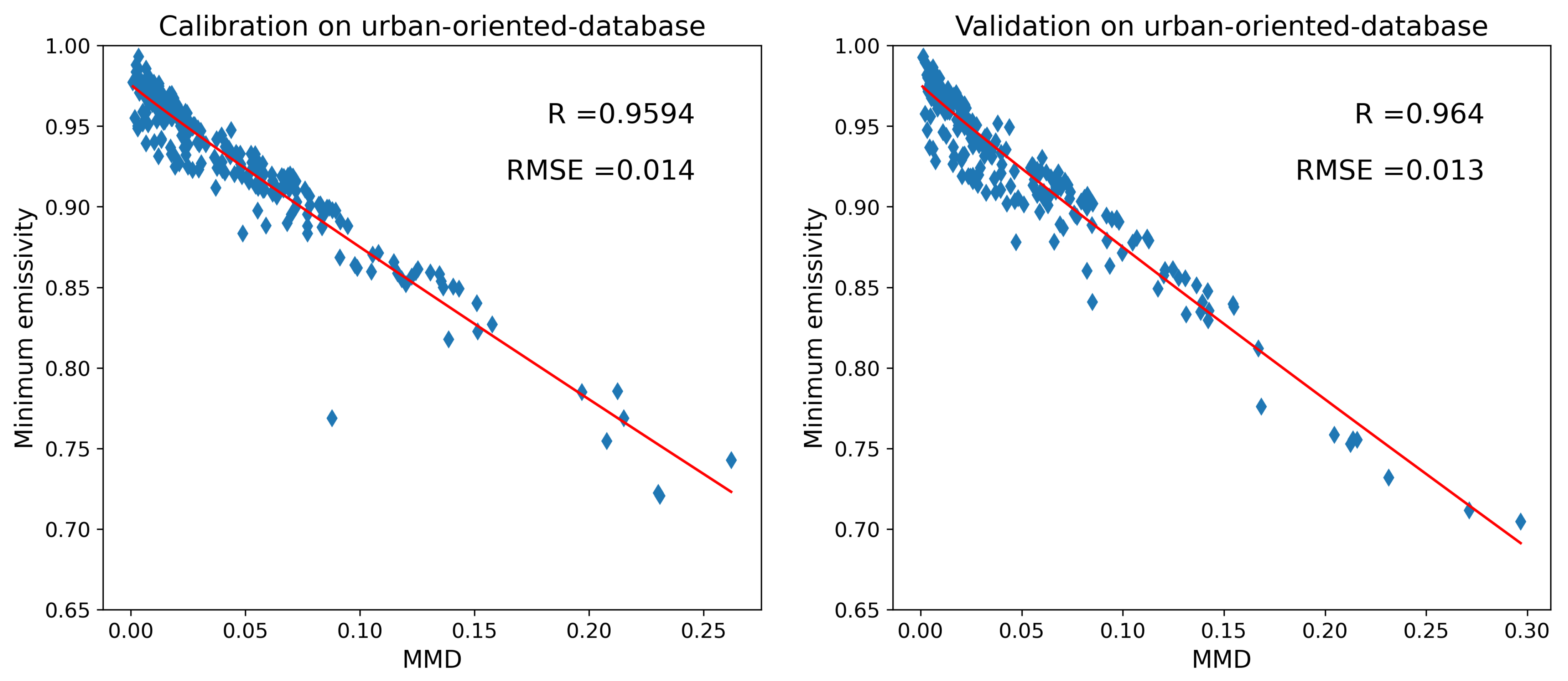
This article proposes two new versions of the TES algorithm based on two new approaches for the study of urban LST. The calibration of the TES algorithm is based on a non-linear regression of an empirical relationship. The first approach considers the calibration with an urban-oriented database in order to retrieve the parameters of the regression. We call this database urban-oriented because it contains similar amounts of both artificial and natural materials compared with the classical databases based on natural materials only. A unique empirical relationship is defined by this database and we call this approach 1MMD TES. The second approach considers two empirical relationships, one for the artificial materials and the other for the natural ones. The urban-oriented database is split in two for calibration. We call this approach 2MMD TES. An a priori under the form of a ground cover classification map is used to associate one observed pixel to the right empirical relationship.
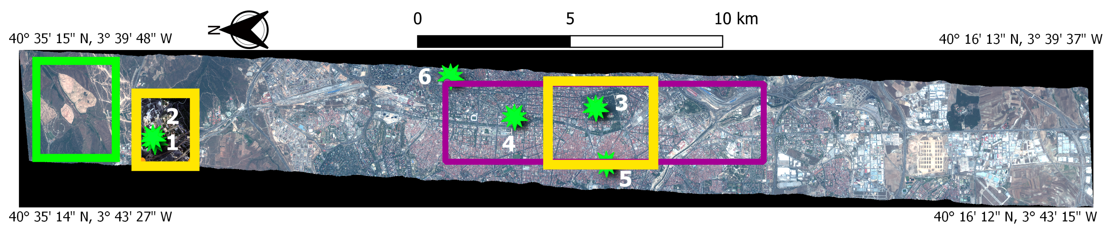
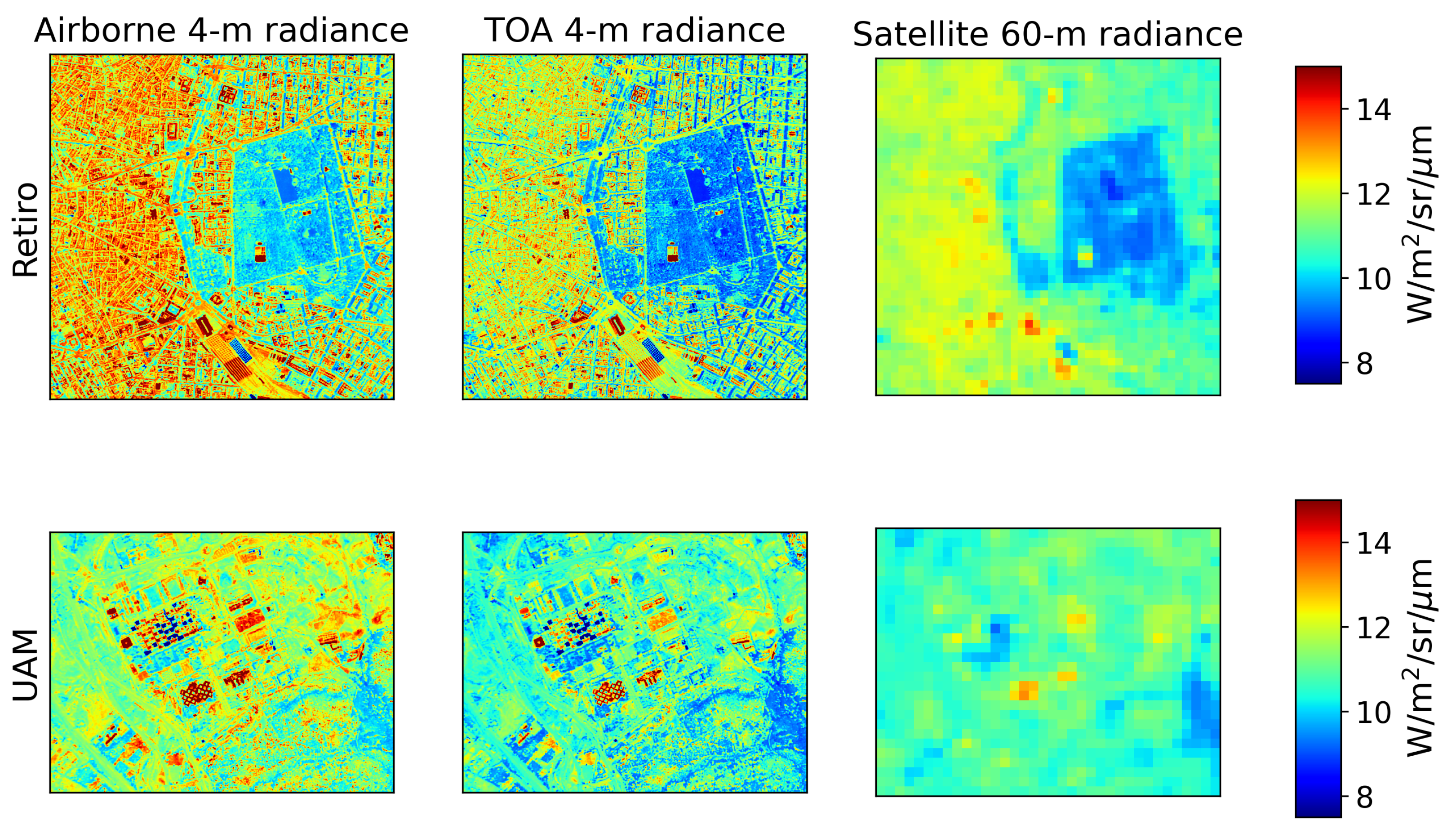
This article uses airborne images over Madrid (Spain) obtained during the ESA-DESIREX (Dual-use European Security IR Experiment) campaign in 2008. Then, from these airborne acquisitions, TRISHNA images at a lower resolution are simulated. The ESA-DESIREX campaign took place in Madrid during the 2008 summer period, with daytime and nighttime radiance images acquired at a 4-m spatial resolution by the AHS (Airborne Hyperspectral Scanner) sensor and ground measurements. These images have been processed to study the SUHI effect over Madrid city using the TES algorithm with seven bands [10,47,61]. These previous works, the configuration of the AHS sensor (10 spectral bands in the TIR range) and the characteristics of the ESA-DESIREX campaign make the dataset a good candidate to prepare the future TRISHNA mission and the development of adapted LST retrieval methods over urban areas by simulating TRISHNA-like images from AHS data.
This study is among the first ones using TRISHNA-like data over urban areas and aims to obtain preliminary performances of this future mission for LST retrieval. It will help the development of algorithms for the future TRISHNA mission, when a maximum of four spectral thermal bands are used with a 60-m spatial resolution. Thus, the performance of two new versions of the TES algorithm, 1MMD TES calibrated with an urban-oriented database and 2MMD TES, is studied in order to highlight their advantages, their limitations and their possible improvements to enhance the accuracy of the retrieved LST.
The following study is divided into six different sections: Section 2 presents the materials: the ESA-DESIREX campaign with both airborne and ground data in Section 2.1, the simulation of TRISHNA-like data in Section 2.2 and the spectral databases to calibrate the TES algorithm in Section 2.3. Then, the TES algorithm is presented in Section 3, focusing on the classical approach in Section 3.1 and our approach in Section 3.2. Section 4 deals with the results, and further discussion is provided in Section 5. Finally, conclusions and future works are highlighted in Section 6.

2. Materials and Methods

2.1. The ESA-DESIREX Campaign: Airborne, Ground and Classification Data

The ESA-DESIREX campaign was an urban experimental campaign that took place in Madrid during the summer period, from the 23 of June to the 6 of July 2008. During this campaign, airborne data were acquired with the AHS sensor operated by the Spanish Institute of Aeronautics (INTA for Instituto Nacional de Técnica Aeroespacial). The AHS sensor is a 80-band radiometer covering the VNIR, SWIR, and TIR spectral ranges. This article focuses on the last ten bands from 71 to 80 in the TIR range. The effective wavelengths in micrometers and the FWHM (Full Width at Half Maximum) for the ten bands of AHS in the TIR range are given in Table 1.
In this work, daytime (around 11 A.M UTC) and nighttime (around 10 P.M UTC) radiance AHS images of the flight line going from north to south for the 28 of June, the 1 of July, and the 4 of July were processed and analyzed (i.e., 6 different images). The spatial resolution is 4 m and all the images were georeferenced [62]. Figure 1 illustrates a RGB image of the flight line going from north to south that was acquired on the 4 of July of 2008. Two areas were chosen for visual analysis: the Retiro Park in the center of Madrid and the Universidad Autónoma de Madrid (UAM) in the peri-urban northern area of the city. The numbers on the Figure 1 are those of the locations of the ground LST measurements, that are described below.
Radiosoundings were made through free or captive balloons that were launched twice a day (daytime and nighttime) recording physical parameters such as pressure, air temperature, relative humidity, wind velocity and wind direction up to 25 km in altitude [62]. The knowledge of these parameters allows retrieving the atmospheric transmittance as well as improving the atmospheric correction of the remote sensing images, which is of high relevance for the TES algorithm [61].
For the ground measurements, calibration and validation sites were selected because of: (i) the stable atmospheric conditions during the ESA-DESIREX campaign, (ii) the low water vapor content, (iii) the homogeneity of both LST and LSE, (iv) absence of shadows and (v) the flat grounds avoiding the impact of the 3D structure on the measured radiance [62]. The sites over the processed flight line were on the one hand: green grass as a cold target in a rugby field (1) and bare soil as a hot target in a soccer field (2), both located at the “Universidad Autonoma de Madrid” (UAM). On the other hand, water at the “Retiro lake” (Estanque Grande del Retiro) (3) as a cold target in the center of the city was used. Surface radiometric temperature, emissivity and downwelling atmospheric radiance were measured on these sites with radiometers such as Heitroniks or a 5-band CIMEL [62]. Ground radiances were measured with a 5-band CIMEL instrument, and during the campaign, the TES algorithm was applied to obtain LST and emissivity measurements for bare soil and green grass. For water, a 1-band radiometer (Heitroniks) was used with an emissivity value of 0.99 [62]. In addition, fixed masts were located along different sites: in a rural/sub-urban zone at UAM (rugby field) (1), in an urban-dense zone at “CSIC” (4) and “Printing” (5) and in an urban-medium zone at “Urbanism Building” (6). These fixed masts measured air temperature, relative humidity and ground radiometric temperature with 1-band radiometers. The radiometric temperature from fixed masts was obtained with 1-band radiometers using the sky irradiance and an emissivity value of 0.9 for artificial surfaces to derive the LST. Table 2 gives the longitude and latitude coordinates of the calibration/validation sites and fixed masts. Four car transects were defined to drive throughout the city of Madrid and its surroundings to measure the LST and they are all covered by the AHS flightlines. The car transect 1 is along the north–south axis, the car transect 2 is in the old center of Madrid, the car transect 3 is in wide space and vegetated areas and the car transect 4 is in wide streets with new buildings and also the highway. The areas crossed by the car transects are not homogeneous in order to better observe the thermal variations. The different car transects are useful for retrieving the SUHI values over different parts of the city.
Figure 2 illustrates the two areas used for visual analysis that are the Retiro Park and the UAM with stars pointing out the locations for calibration and validation. These areas were chosen because they include both natural and artificial materials and some validation points. The Retiro Park is an urban dense zone, and the UAM is a rural sub-urban zone.
Lastly, a supervised classification-based approach was applied during ESA-DESIREX on daytime AHS images for the 4 of July, with ground measurements to define the endmembers spectra and the Maximum Likelihood used as the decision rule. Twelve classes were selected with a 73% kappa coefficient: water (lakes and swimming pools), trees, green grass, bright and dark bare soils, roads with asphalt, other roads and pavements, roofs with red bricks/tiles, roofs with asphalt, roofs with concrete and roofs with metal. The details for this classification can be found in [63]. Figure 3 shows the classification map obtained at a 4-m resolution over the Retiro Park and the UAM with the legend for every classified type of material. Further information about the ESA-DESIREX campaign and its results over the city of Madrid can be found in the ESA-DESIREX 2008 final report [62].

2.2. Simulation of TRISHNA-like Data

2.2.1. Radiance Images

In the TIR range (8–14 μ m), the radiance at the sensor-level in a specific spectral band and close to nadir is expressed as:
L λ , s e n s o r = τ λ a t m , s e n s o r L λ , B O A + L λ a t m , s e n s o r Wm 2 μ m 1 sr 1
where λ is the considered wavelength, τ a t m , s e n s o r the atmospheric direct transmissivity between ground and sensor (the diffuse transmissivity is negligible in the thermal domain), L λ a t m , s e n s o r the upwelling path radiance and L λ , B O A the radiance at the Bottom Of Atmosphere (BOA). The L λ , B O A can be expressed as:
L λ , B O A = L λ , s u r f a c e + [ 1 ε λ ] L λ a t m W m 2 μ m 1 sr 1
Furthermore,
L λ , s u r f a c e = ε λ L B B ( T s ) W m 2 μ m 1 sr 1
where L λ a t m is the downwelling atmospheric radiance, L λ , s u r f a c e is the radiance at the surface, ε λ is the equivalent surface emissivity and L B B ( T s ) is the radiance defined by the Planck’s law for a black body at the temperature T s . Thus, the LST ( T s ) is obtained by inverting the Planck’s law:
T s = c 2 λ ln ( c 1 λ 5 L λ , s u r f a c e ε λ + 1 ) K
With c 1 and c 2 being the constants in the Planck’s law, c 1 = 1.19104 W μ 4 m 2 sr 1 and c 2 = 14387.7 μ m K . All the quantities in Equations (1)–(4) depending on the wavelength are mentioned as equivalent: they are integrated according to the spectral response of the considered sensor and normalized by it.
As the number, position and bandwidths of the four thermal spectral bands for TRISHNA were not determined yet when the study was made, AHS bands were used to simulate TRISHNA ones. Four AHS bands were chosen according to the closeness of the central wavelength compared with the known central wavelengths for the TRISHNA sensor: AHS band 72 at 8.18 μ m, 73 at 9.15 μ m, 76 at 10.59 μ m and 78 at 11.78 μ m [26]. Figure 4 summarizes the simulation methodology.
  • Step 1: From airborne level to TOA (Top of Atmosphere) level:
    To model the attenuation through the atmosphere, Equation (1) can be expressed for both the airborne level and satellite level, leading to a linear relationship between the AHS radiance and the TOA radiance. Both the slope and the intercept of this relationship depend only on the atmospheric conditions and the observation angle (nadir is considered in this study). Details of the calculation for both the slope and the intercept can be found in [64]. Simulations are performed with the radiative transfer code COMANCHE using the ESA-DESIREX atmospheric profiles, 75 synthetic emissivity spectra and 6 temperatures for each spectrum [65,66]. The temperature range is 273–335 K and the emissivity range is 0–1 to have a dense representation of the earth surface spectra. The slope and intercept parameters of the linear relationship are retrieved with the least squares fitting and then can be applied to the AHS images to obtain the radiances at the TOA level.
  • Step 2: Spatial aggregation (undersampling) and noise:
    The undersampling is made with a Function Transfer Model (FTM) and SNRs (Signal to Noise Ratios) that were defined according to the first TRISHNA sensor characteristics. The FTM is considered exponential in this spatial aggregation procedure.
  • Step 3: Atmospheric correction to obtain the BOA radiance:
    The atmospheric coefficients integrated into the four selected spectral bands are kept in order to perform the atmospheric correction allowing to pass from TOA to BOA radiances before applying the TES algorithm (see Equation (1). These coefficients are retrieved with the radiative code COMANCHE thanks to the ESA-DESIREX atmospheric profiles.
In the end of this processing, daytime and nighttime BOA radiance maps at 4 and 60 m spatial resolutions are obtained. Figure 5 shows AHS radiance and TOA radiance at 4 m resolution together with TOA radiance at 60 m resolution for band 72 of AHS (band 1 of TRISHNA). Thus, it allows illustrating the different steps of the methodology. LST retrieval through the TES algorithm is described in Section 3.

2.2.2. Ground Cover Classification Map

The 4-m ground cover classification map was aggregated at 60 m by using the nearest neighbor approach with k = 15 neighbors and keeping the most prevalent class. Figure 6 shows the obtained 60-m classification map from the 4-m one. It is worth noting that this approach considers 60-m pixels as pure. This consideration is later discussed in Section 5.

2.3. Urban-Oriented Database for TES Calibration

This article focuses on the future TRISHNA sensor and proposes an urban-oriented database to calibrate the TES algorithm. Indeed, a database containing both natural and artificial surface emissivities is needed to perform a representative calibration for urban environments. In this study, emissivities were recovered from those spectral databases: ECOSTRESS (formerly ASTER, [67,68]) for artificial surfaces and bare soils, CAPITOUL [69] (laboratory measurements over artificial surfaces taken in Toulouse, France), SLUM [70] (ground measurements over artificial surfaces in London, UK), MODIS [71] and IPGP [72] databases. Whether the considered surfaces are artificial or natural, the data processing was slightly different. For natural surfaces, a similar approach to [73,74,75] was adopted:
  • All spectra that did not cover the spectrum from the VNIR to the TIR ranges were rejected.
  • To avoid any redundancies, the SAM (Spectral Angle Mapper) distance between each pair of spectra was computed [76]. To define any redundancy or not, the threshold was set to 1° according to the study made by [75].
  • The PRO-SAIL (Scattering by Arbitrarily Inclined Leaves combined with PROSPECT) model was used to simulate mixed spectra of soil and vegetation at the top of the canopy with different values of Leaf Area Index (LAI) and Average Leaf Angle [77]. More than 60,000 spectra result from the process. This simulation of natural surfaces was chosen because: (i) it is more representative of the pixel that is observed at the sensor level, (ii) it takes into account the canopy effect and iii) the TES algorithm was applied on this database with experimental satisfactory results [74]. Natural surfaces in our spectral databases are thus composed of pure and linearly mixed spectra of bare soil and vegetation. The PROSPECT model has been parametrized following [73,74,75].
  • The SAM distance with a threshold of 1° is computed in order to avoid any redundancies.
  • All spectra with an equivalent emissivity lower than 0.7 between 10 and 12 μ m were rejected.
For artificial surfaces, the following methodology was retained:
  • All spectra that did not cover the spectrum from the VNIR to the TIR ranges were rejected.
  • For the CAPITOUL database, the tiles were rejected as the laboratory measurements showed some errors.
  • The SAM distance with a threshold of 1° is computed to avoid any high redundancies.
  • All spectra with an equivalent emissivity lower than 0.7 between 10 and 12 μ m are rejected.
Note that no low emissivity materials (lower than 0.7) have been used because of the known poor performance of the TES algorithm for these materials [40,78].
In the end, our spectral database consists of 266 emissivities of natural materials and 236 emissivities of artificial materials. In detail, artificial materials account for 47% and natural ones for 53%, which makes the spectral database representative of the urban areas and the rural surroundings. Next, this database is split into calibration and validation datasets. For natural surfaces, a random sampling is made among the 266 emissivities, while for artificial surfaces, a random sampling is made among the different spectral databases of artificial materials in order to avoid any kind of prevalence of a field instrument compared to another one. Finally, two independent databases with 251 emissivities each were used for calibration and validation, respectively. More precisely, each dataset contains 133 spectra of natural surfaces and 118 of artificial ones.
Instead of looking for a heterogeneous TES calibration spectral dataset able to represent all the different surfaces appearing in an urban satellite image, two sub-datasets characterizing, respectively, artificial and natural surfaces can be built. We call these databases artificial-surface-oriented and natural-surface-oriented, respectively. Thus, the above urban-oriented spectral database can be divided into the artificial-surface-oriented one with 236 emissivities and the natural-surface-oriented one with 266 emissivities. Newly, these databases can be split into two independent calibration and validation datasets. This original approach leads to material-specific calibration of TES.

3. LST Retrieval with the TES Algorithm

For a number of N spectral bands, there are N observed radiances and N + 1 unknowns: N emissivities + 1 LST, consequently, the system is undetermined. Different methods use approximations or a priori information to derive the system unknowns. These methods can be divided into different categories whether they use one single band, two bands or more, a combination of daytime/nighttime observations or multi-angle observations. A review of the LST retrieval methodologies can be found in [79,80,81,82]. In this work, we focus on the TES algorithm that uses an empirical relationship in order to solve the system because this algorithm is commonly used and it can be applied with more than three bands.

3.1. The Classical Approach: TES with One MMD Relationship or 1MMD TES

The TES algorithm has first been introduced in [36] for ASTER data processing and is based on three modules: NEM for Normalized Emissivity Method, RATIO and MMD for Maximum-Minimum Difference. Thus, TES jointly retrieves LSE and LST [83]. This algorithm can be applied to any sensor with more than three thermal bands. The first module, NEM, uses an initial emissivity value (here 0.99) and iteratively corrects it. The RATIO module normalizes the new emissivities by the average of all found emissivities in all the thermal bands. This preserves the shape of the spectrum and minimizes the sensitivity to errors in temperature estimation. The third module converts normalized emissivities into actual emissivities using the empirical relationship called MMD relationship. The MMD relationship is expressed as:
ε m i n = a + b M M D c
With ε m i n the minimum equivalent emissivity and MMD the maximum difference between equivalent emissivities in the considered spectral thermal bands (in this study, bands 72, 73, 76 and 78 of AHS). The values of the coefficients a, b and c needed for the TES algorithm are retrieved with the spectral databases presented in Section 2.3. The system is non-linear and non-convex so a Levenberg–Marquard minimization was used to retrieve the coefficients. TES is applied directly on BOA radiance L λ , BOA , and so an atmospheric correction is needed, see Section 2.2.

3.2. The TES Algorithm with 2MMD Relationships or 2MMD TES

Two independent TES algorithms are calibrated on different specific material sub-datasets, leading to a artificial-surface-oriented TES and a natural-surface-oriented TES, see Section 2.3. Each calibration is performed independently following the scheme described in Section 3.1. Combining this approach with a ground classification map at the resolution of the TIR bands of the satellite, we can locally apply an adapted TES to each pixel. We call this approach the 2MMD relationship’s TES algorithm, i.e., 2MMD TES.
The last step requires to chose how to associate the ground classification map to the appropriate MMD relationship. It can appear trivial to separate artificial and natural materials, but it is worth noting that spectrally, both groups can overlap, and some artificial materials can exhibit a spectrum close to natural ones and vice versa. Thus, each class of the ground classification map was analyzed regarding the ground LSEs that allowed the classification process, the results from the 7-band TES used for AHS data and the results from the 1MMD TES. All these observations showed that the “bright bare soil” class had a higher LSE variability and a lower minimum emissivity than the other natural classes. Consequently, this peculiar class was considered as an outlier for the natural MMD relationship. The natural MMD relationship is then applied for the classes 1, 2, 3, 4 and 6, and the artificial MMD relationship for the other classes, see Figure 3 and Figure 6.

3.3. Calibration and Validation of the 1MMD TES and the 2MMD TES

Figure 7 shows the statistical fits of the MMD relationship (Equation (5)) for the calibration dataset and the validation dataset that were used for the 1MMD TES with the urban-oriented-database. The MMD relationship obtained is illustrated with a red line. For the calibration dataset, the MMD relationship provides an RMSE value of 0.014, a standard deviation of 0.014, and a correlation coefficient R of around 0.96. For the validation dataset, the RMSE is 0.013, the standard deviation is 0.013 and the correlation coefficient R is 0.96. These values lead to an error on the LST of about 1 K. Similar performances were found in the literature. Thus, the study from [61] with 299 natural materials gives a standard deviation value of 0.019 and a correlation coefficient R of 0.96. The study from [10] on AHS images over urban areas with a database using 108 natural materials gives a standard deviation of 0.005 and a higher correlation coefficient R of 0.997. The study of [78] using 54 artificial materials gives an RMSE value of 0.024, which is higher than our RMSE value of 0.013. Therefore, mixing artificial and natural materials does not degrade the performances of the MMD relationship for the 1MMD TES compared with other studies that used only natural or only artificial materials in the calibration phase. It is worth noting as well that the aforementioned studies used more than four spectral bands. With these observations, the urban-oriented developed database including both natural and artificial materials appears thus to be suitable to retrieve LSTs over urban areas.
Figure 8 shows the two MMD relationships statistical fits of (1) the artificial-surface-oriented and (2) the natural-surface-oriented databases and both for their corresponding calibration and validation dataset. For both cases, the MMD relationship is illustrated with a red line. For artificial materials, the calibration dataset gives an RMSE value of 0.015, the standard deviation is 0.015, and the correlation coefficient R is almost 0.96, similarly to the results obtained on the urban-oriented database. For the validation dataset, the RMSE is 0.014, the standard deviation is 0.014 and the correlation coefficient R is around 0.97. For natural materials, the calibration phase gives an RMSE value of 0.004, the standard deviation has nearly the same value and the correlation coefficient is slightly higher than 0.99. The validation phase gives an RMSE value of 0.005, a standard deviation of 0.005 and a correlation coefficient of 0.99, which is similar to the results found in [10] that used seven bands. Thus, it can be highlighted that with only four bands, the performances of our 2MMD relationships become similar to those of a single MMD relationship with seven bands. Moreover, comparing Figure 7 and Figure 8, the minimum emissivity can be underestimated for the natural materials when only one MMD relationship is used, which can lead to an overestimation of the retrieved LST. In addition, it is seen that the artificial materials used in our urban-oriented database tend to have a lower minimum emissivity than the natural materials, as well as a larger spectral contrast, in accordance with their high spectral variability. Separating both kinds of materials allows providing a more suited MMD relationship to retrieve the LST. From now on, to highlight the number of spectral bands, the 2MMD TES is called 2MMD-4-band TES, the 1MMD TES is called 1MMD-4-band TES and the 7-band TES used for comparison is called 1MMD-7-band TES. Table 3 provides the coefficients of the MMD relationship according to the database and the number of bands.

3.4. Performance Assessment of the LST Retrieved by the 1MMD-4-Band TES and the 2MMD-4-Band TES

LST maps obtained at a 4-m resolution from the 1MMD-7-band TES by [10,59,78] were used as references to evaluate and compare the performance of both 1MMD-4-band and 2MMD-4-band TES algorithms from AHS data at a 4-m spatial resolution. While [10,59,78] used a classical calibration-validation database, the two versions of the TES algorithm, 1MMD-4-band and 2-MMD-4-band, use the aforementioned urban-oriented database, and thus, this comparison will allow to better understand the advantages and limitations of such a database. At the satellite level, a temperature upscaling based on the Stefan–Boltzmann’s law and applied on each 4-m LST map is considered as reference. Consequently, the 4-m LST maps of this study are spatially aggregated to 60 m to compare with TRISHNA-like LST maps obtained at a 60-m spatial resolution. The comparison of the TRISHNA-like LST with the aggregated one for each method is used to better understand how the decrease in spatial resolution impacts each method’s performances.
To quantitatively compare the images, the Root Mean Square Error (RMSE), the Mean Bias Error (MBE) and the Structural Similarity Index (SSIM) were chosen (all formulas for theses indexes can be found in [64]). First-order statistics of the LST maps were computed to help in the analysis, i.e., the mean and the standard deviation. Lastly, the local/pixel per pixel difference was used to highlight the largest differences between both 1MMD-4-band and 2MMD-4-band TES algorithms. In addition, as ground measurements are available (Section 2.1), local comparisons can be made by computing the RMSE and MBE between ground measurements and the corresponding pixel in the 4-m LST images.

4. Results

The 4 of July 2008 was chosen to show the LST maps provided in this section. Similar visual and quantitative results were found for the other acquisitions. However, the statistical analysis for the comparison of TES LSTs with ground measurements as well as the SUHI values are performed on all the acquisitions.

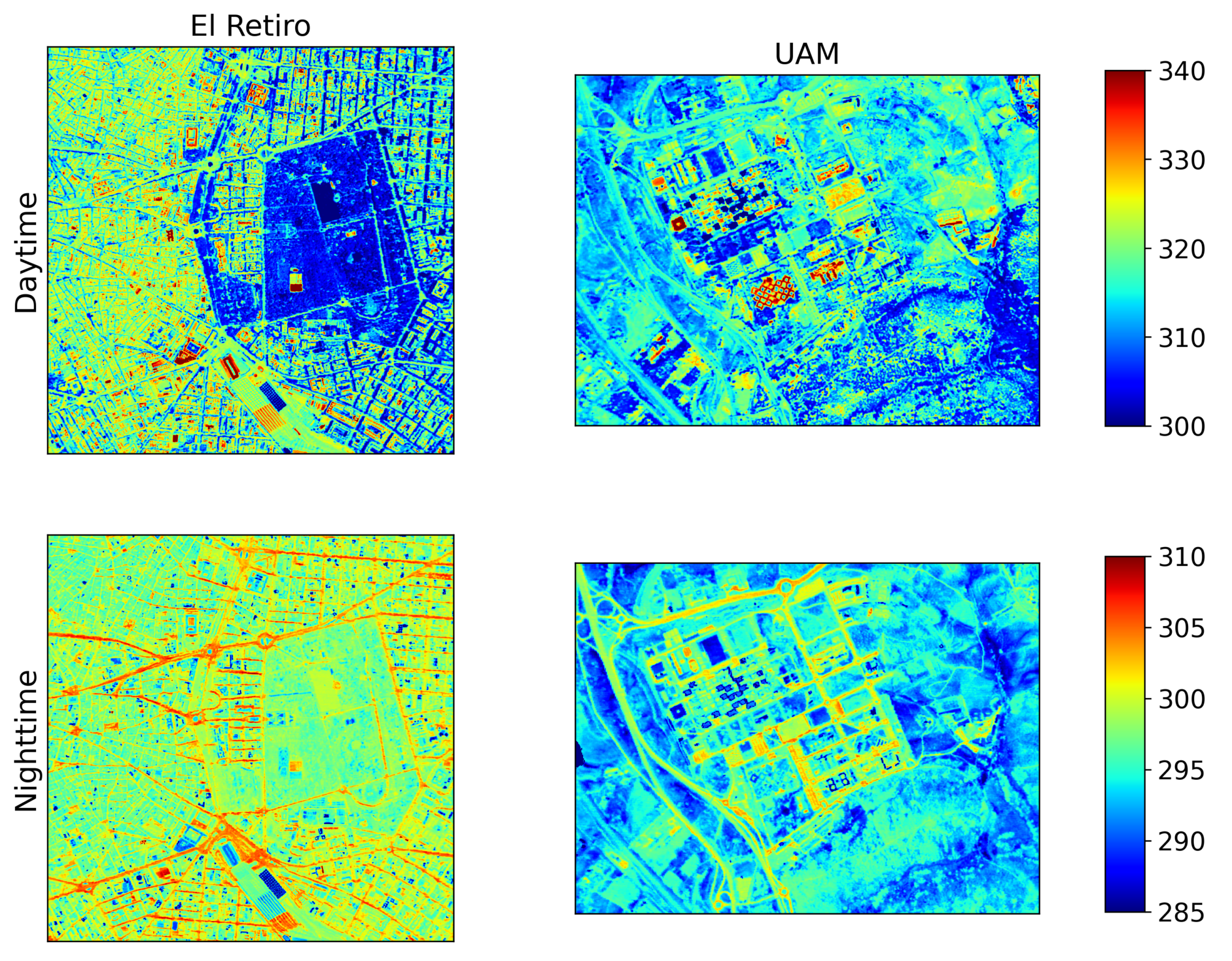
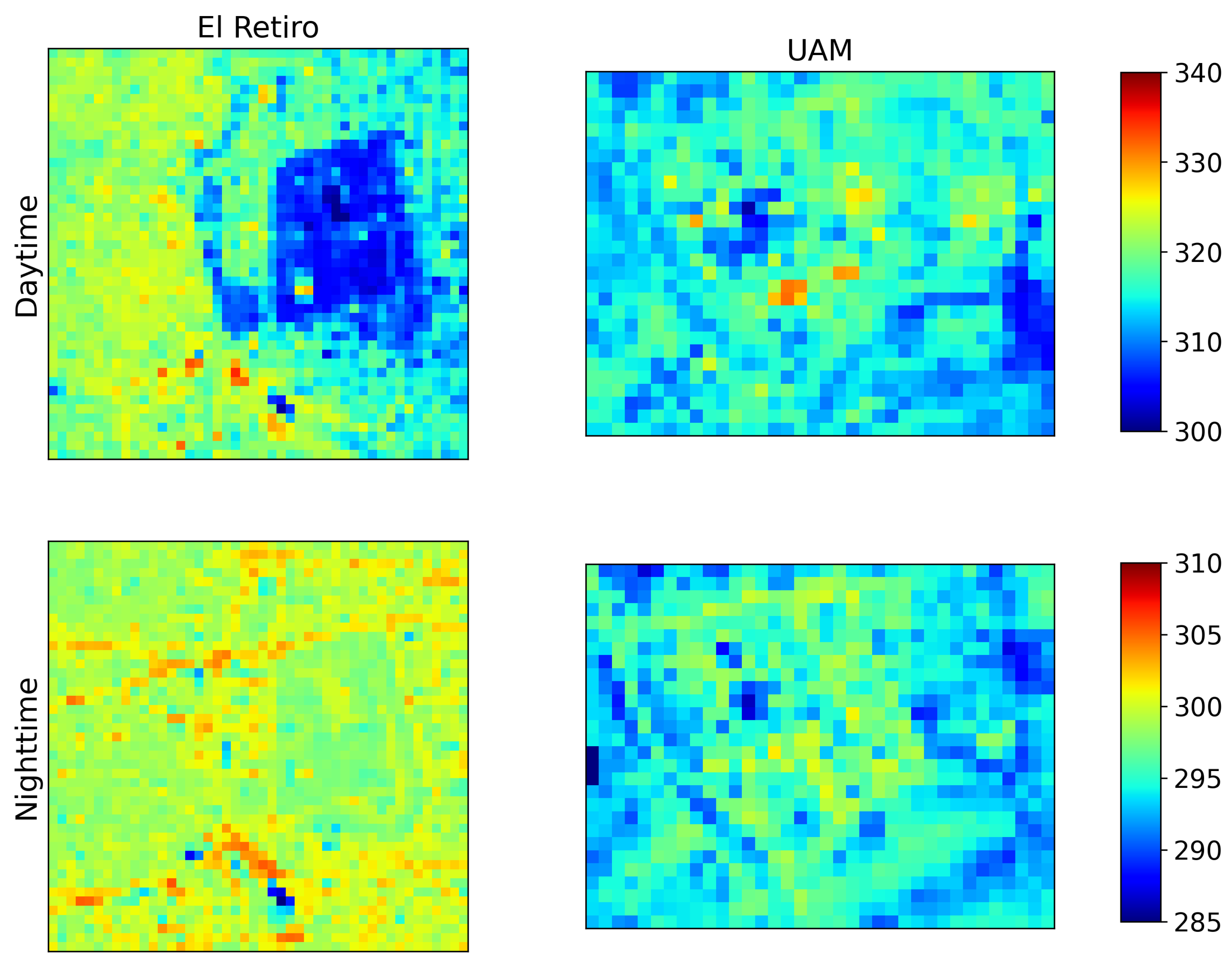
4.1. LST Map Reference

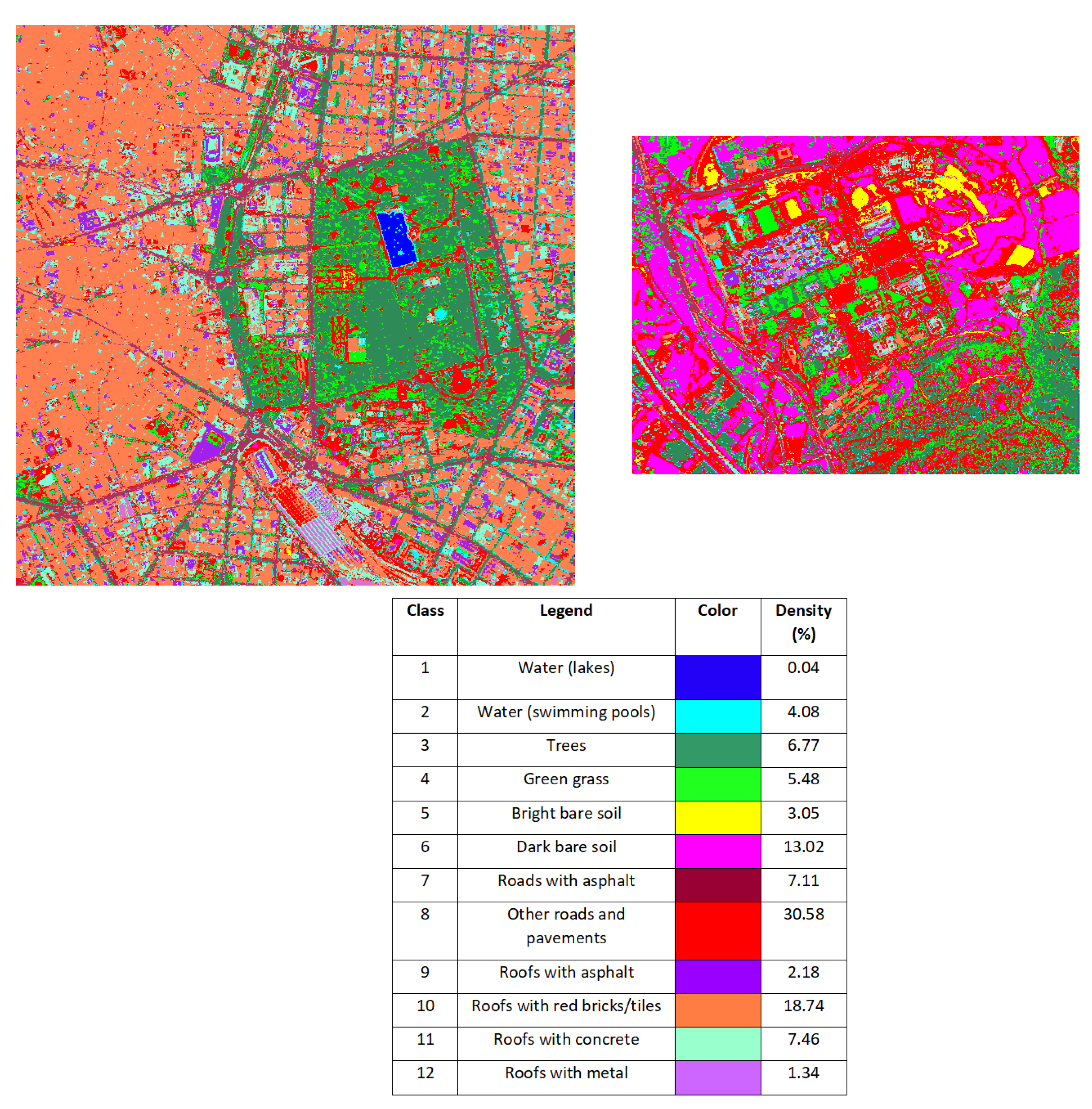
Figure 9 shows the daytime and nighttime LST reference map in K at 4 m for the 4 of July over the two studied areas (the Retiro Park and the UAM). During the daytime, for both the Retiro Park and the UAM, spatial variations of LST are easily noticeable. For the Retiro Park, the Retiro lake presents the lowest temperature around 300 K, the vegetated area around 310 K, the left part of the Retiro Park is between 300 and 320 K and the right part of the Retiro Park is between 310 and 320 K. For the UAM, the rugby field is between 300 and 310 K, the soccer field around 315 K and some building roofs have high LSTs around 335 K. The surroundings of the UAM have an LST ranging from 300 to 325 K, with the highest LSTs over bare soil waste ground (classified as “dark bare soil”), and the coolest LSTs over vegetated areas (classified as “trees” or “green grass”). The roads have a LST value of around 315 K.
During the nighttime, for the Retiro Park, the water lake does not present LST variations between day and night with LST ≈ 300 K in agreement with the heat capacity of water. The streets have the highest LSTs around 305 K, and some other roads have a LST value of around 302 K. The vegetated area of the Retiro Park is around 298 K. However, for both daytime and nighttime, some unusual patterns can be seen with low LSTs, especially on one roof of the Atocha train station. For the UAM, unusual patterns can be seen in the center of the image within the campus with low LSTs under 285 K. Otherwise, the streets have the highest LSTs around 302 K and surroundings have an LST value ranging from 285 to 297 K. It is worth noting that the observed unusual patterns are seen during daytime and during nighttime. This observation is discussed in Section 5.1.
Table 4 gives the mean and the standard deviation of the LST. Between the Retiro Park and the UAM, the mean LST difference is 1.6 K and the std difference is 2.3 K for daytime. The mean LST difference is 4.4 K for nighttime and the std values are the same. Between daytime and nighttime, the mean LST difference is 17.3 K for the Retiro Park and 20.1 K for the UAM. The std difference is 5.5 K for the Retiro Park and 3.2 K for the UAM.

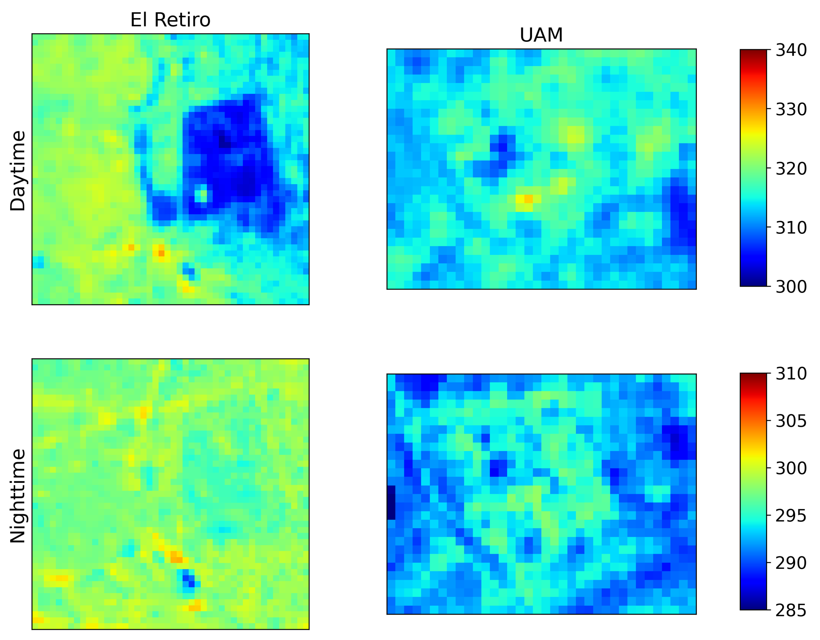
4.2. LST Retrieval with the 1MMD-4-Band TES and the 2MMD-4-Band TES with TRISHNA-like Spectral Configuration at 4 m

Figure 10 and Figure 11 show the daytime and nighttime LST in K for both studied areas as retrieved with the 1MMD-4-band TES and 2MMD-4-band TES, respectively. For a statistical analysis of performances, Table 5 shows the RMSE, MBE and SSIM between the 1MMD-7-band TES from [10,59,78] and the 1MMD-4-band TES and the 2MMD-4-band TES of this study. This table also shows the mean and standard deviation of the LSTs obtained with the 1MMD-4-band TES and the 2MMD-4-band TES.
During both daytime and nighttime and for both the Retiro Park and the UAM, the obtained LST maps are similar to the LST map reference, see Figure 9, Figure 10 and Figure 11. Thus, the same observations can be made.
Looking at the mean and standard deviation of the LST in Table 5, for the 1MMD-4-band TES, the mean LST difference is 1.8 K and the std difference is 2.5 K for the daytime between the Retiro Park and the UAM. The mean LST difference is 4.5 K and the std difference is 0.4 K for nighttime. For the 2MMD-4-band TES, the mean LST difference is also 1.8 K and the std difference is 2.4 K for daytime between the Retiro Park and the UAM. The mean LST difference is 4.6 K for nighttime, and the std difference is 0.1 K.
Between daytime and nighttime, for the 1MMD-4-band TES, the mean LST difference is 17.7 K for the Retiro Park and 20.5 K for the UAM. The std difference is 5 K for the Retiro Park and 2.9 K for the UAM. For the 2MMD-4-band TES and between daytime and nighttime, the mean LST difference is 17.7 K for the Retiro Park and 20.5 K for the UAM, just like the 1MMD-4-band TES. The std difference is 5.1 K for the Retiro Park and 2.8 K for the UAM.
These differences are similar for all TES algorithms, meaning that there is a physical coherence between the three versions. Considering the comparison with the LST map reference, during the daytime, the RMSE values are lower for the 2MMD-4-band TES than for the 1MMD-4-band TES of 0.22 K for the Retiro Park and 0.06 K for the UAM, meaning that there are larger discrepancies between the 1MMD-4-band TES and the LST reference. However, the MBE values are lower for the 1MMD-4-band TES than for the 2MMD-4-band TES. Both methods tend to retrieve a higher LST than with the 1MMD-7-band TES because the MBE is negative and the 2MMD-4-band TES over the studied areas provides higher mean LSTs than the 1MMD-4-band TES. It is important to remark that the MBE is a signed metric and so underestimations and overestimations of LST can compensate, leading to an MBE closer to zero. This can be the explanation of the better results for the 1MMD-4-band TES. The SSIM index is high as the value is 0.98 for both areas and methods.
During the nighttime, the 2MMD-4-band TES provides a higher RMSE value higher of 0.27 K than the 1MMD-4-band TES for the UAM, but the RMSE value is lower, 0.17 K, for the Retiro Park. Looking at the MBE, values are lower for the 1MMD-4-band TES than for the 2MMD-4-band TES. The MBE values are lower than during the daytime, which can be explained by the absence of solar irradiance, i.e., the smaller variances in LST during the night. The SSIM values are very similar between daytime and nighttime, with little difference between the 1MMD-4-band TES and the 2MMD-4-band TES.
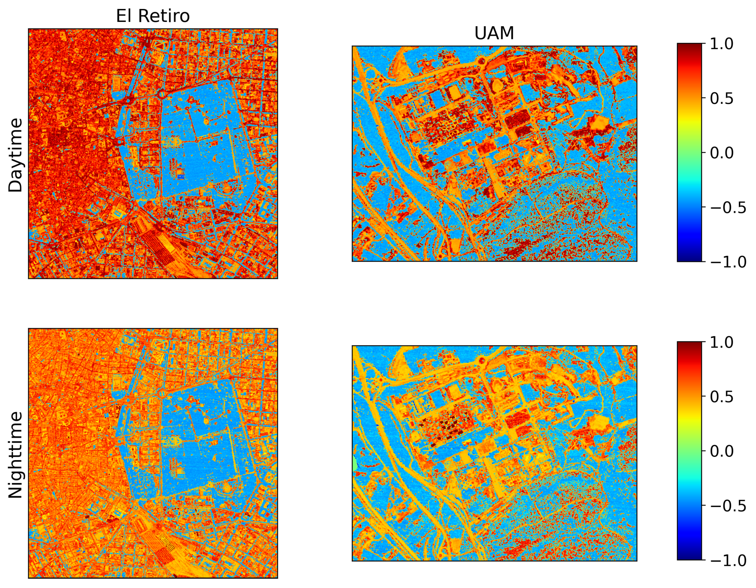
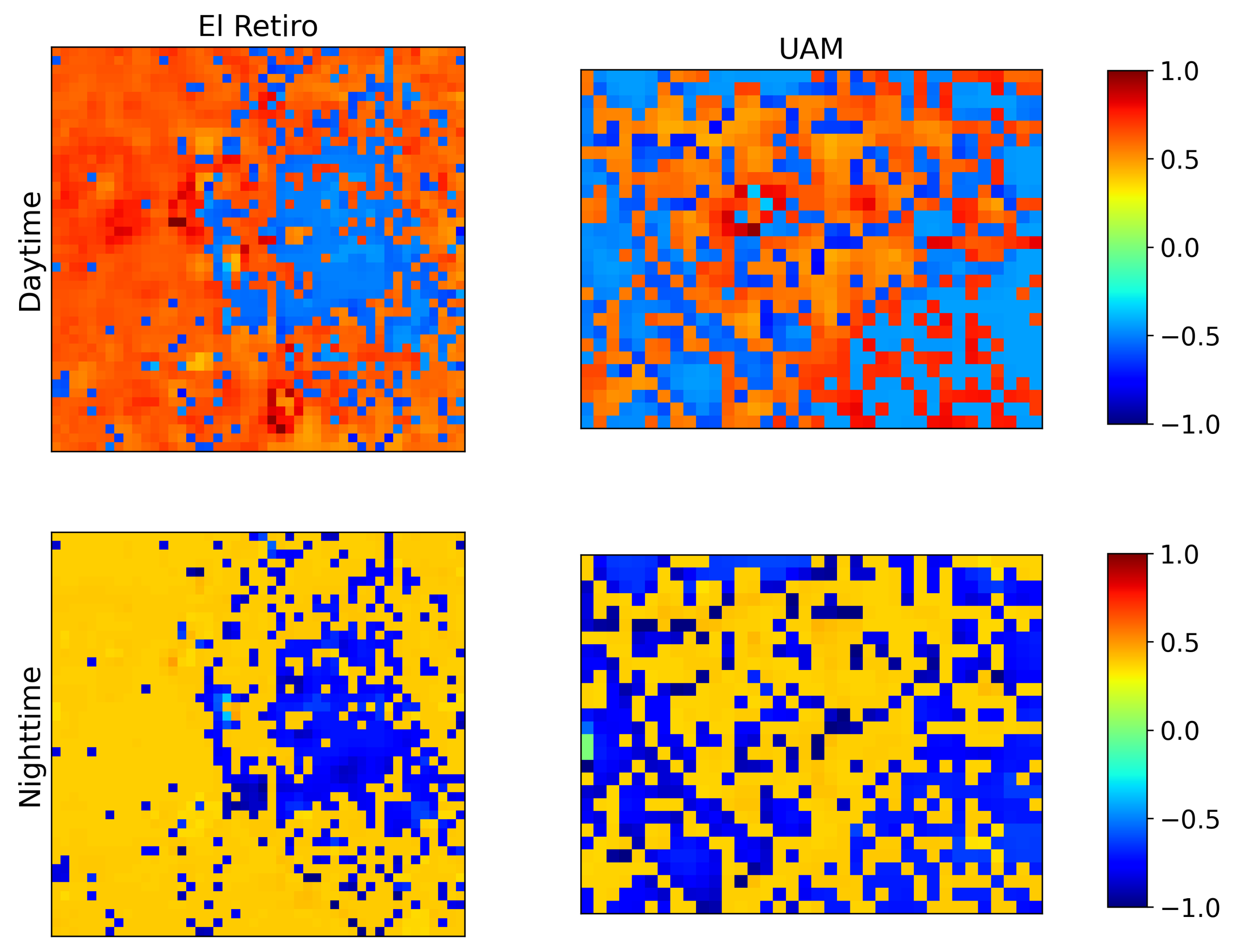
Lastly, Figure 12 shows the pixel per pixel difference between the 2MMD-4-band TES and the 1MMD-4-band TES to highlight the pixels where the difference is high. It can be observed that during the daytime and nighttime, the difference is larger for artificial surfaces, especially the streets and the dense area at the left of the Retiro Park, and the classes “other roads and pavements” and “roofs with metal” for the UAM, with a difference of around 1 K for daytime and between 0.5 and 1 K during the nighttime. For the natural surfaces, such as the vegetated area of the Retiro Park, the water lake and the bare soils or trees, the difference is around −0.5 K for both daytime and nighttime, in agreement with the observations in Figure 7 and Figure 8. Indeed, the 1MMD-4-band TES can overestimate the LST for natural materials. Thus, the 2MMD-4-band TES tends to be the optimal method to retrieve the LST for both kinds of materials. To go in deep with this observation, the comparison with ground LSTs is useful. It will allow assessing which TES algorithm is the most optimal.

4.3. Comparison with LST Ground Measurements

In order to validate the retrieved LSTs at 4 m, a comparison with ground measurements is performed. Two cold targets and four hot targets are chosen: green grass, water, bare soil and three different roofs located in different zones, see Figure 1. Ground LST measurements are selected according to the closeness in time with the daytime and nighttime flights. It gives a total of 30 measurements to compare ground LSTs and retrieved ones for all the acquisitions.
Table 6 and Table 7 show the comparison between ground LSTs and the three versions of the TES algorithm (1MMD-4-band TES, 2MMD-4-band TES and 1MMD-7-band TES from [78]), for the 4 of July, daytime and nighttime, respectively. A star points out the closest retrieved LST to the ground LST. During the daytime, the 1MMD-7-band TES provides the closest LST for the cold target “green grass” and the hot target “bare soil”. On the other hand, for the three artificial materials located at the roofs as well as for the water lake at the Retiro Park, the 2MMD-4-band TES has the best performance. Thus for artificial materials, the 2MMD-4-band TES is the optimal method in this study. During the nighttime, the 2MMD-4-band TES outperforms the other methods for four out of five targets, because the cold target “water” was not measured this night. Again for the hot target “bare soil”, the 1MMD-7-band TES provides the closest LST.
For both daytime and nighttime, the 1MMD-4-band TES never performs better. However, the differences are not very large and it can be seen that for artificial materials, the 1MMD-4-band TES is closest to the ground LSTs than the 1MMD-7-band TES except for the “Urbanism” site during the nighttime, with only 0.1 K between the 1MMD-7-band TES and the 1MMD-4-band TES.
It is worth noting that some significant errors remain over the artificial materials for the three different versions of the TES algorithm. This observation is discussed in Section 5.1.
In Table 8, we decided to compare retrieved and ground LSTs by combining all the six available remote sensing acquisitions and focusing on daytime, nighttime, artificial and natural surfaces separately. Thus, Table 8 gives the RMSE and MBE values in K for all the acquisitions, between ground LSTs and retrieved LSTs from each method, separating daytime, nighttime, artificial and natural materials. The same observations can be made: the 2MMD-4-band TES provides the best performances except for the natural materials where the 1MMD-7-band TES is better. However, for artificial materials and globally, the 2MMD-4-band TES provides better results because the RMSE decreases by 1.6 K over artificial materials and 1 K globally compared with the 1MMD-7-band TES and decreases by 0.5 and 0.4 K compared with the 1MMD-4-band TES.

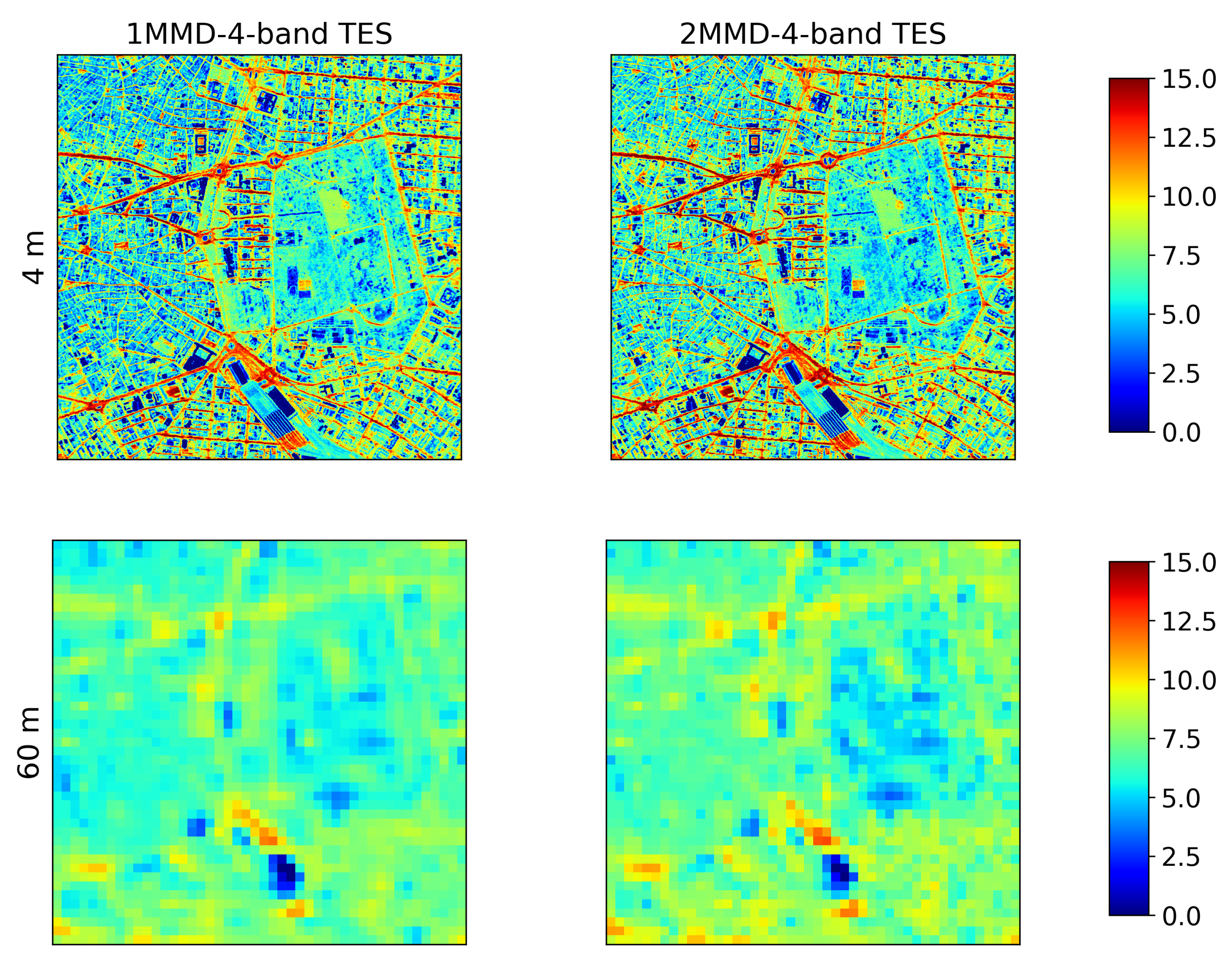
4.4. LST Retrieval in the TRISHNA Framework: 60 m

Figure 13 and 
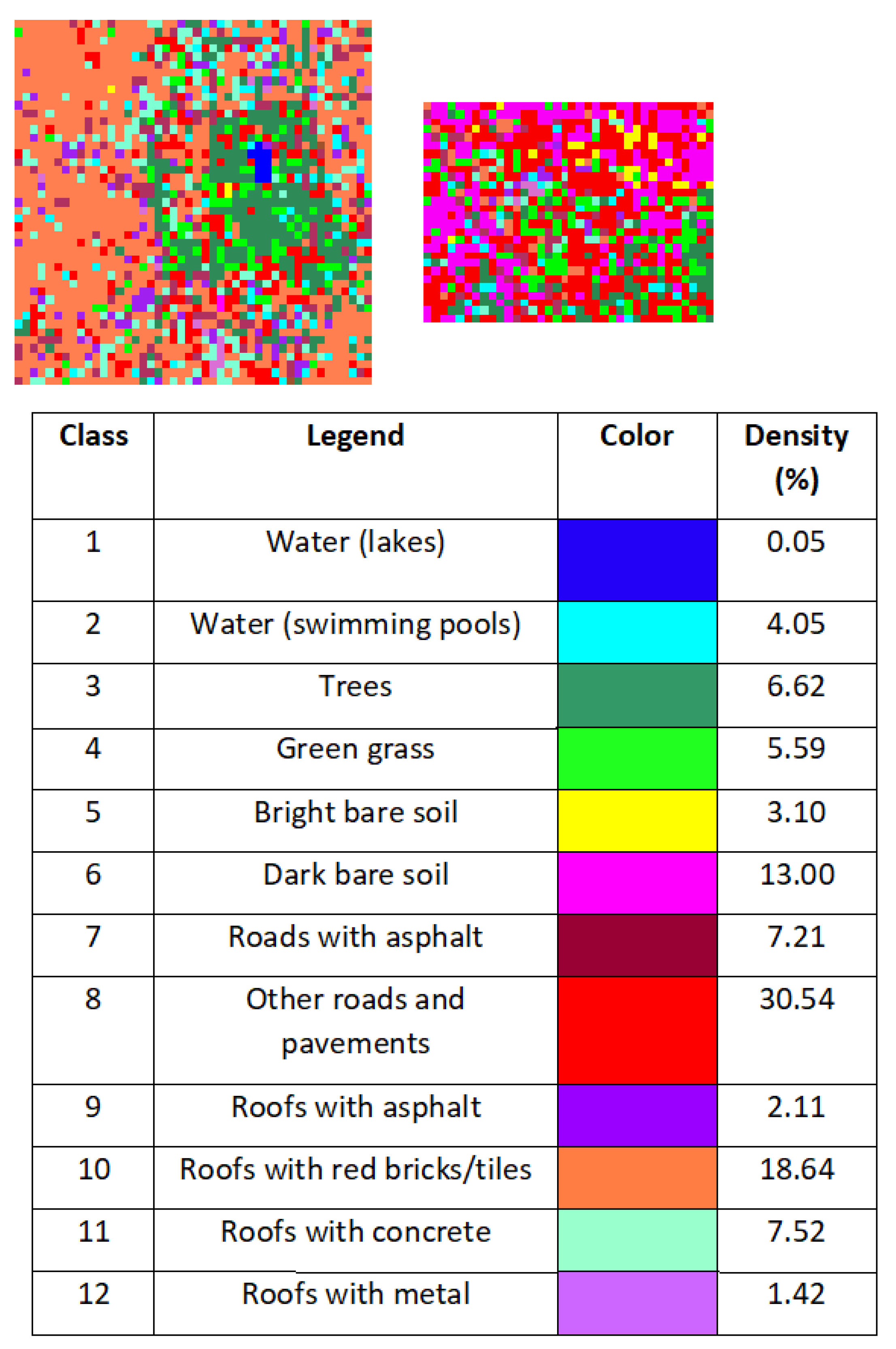
Figure 14 show the 60-m LST maps obtained by aggregating with the Stefan–Boltzman’s law, the retrieved LSTs from the 1MMD-4-band TES and the 2MMD-4-band TES at 4 m. In both figures, LST maps of the Retiro and the UAM during the daytime and nighttime are shown. Visually, the aggregation of both methods provides similar LST maps. The same observations as at 4 m about the spatial patterns can be made. In the Retiro Park area, the water lake and the park are well discernible, as well as roads during the nighttime. For the UAM, the university structures are less visible due to aggregation. However, natural landscapes and some hot points (such as the parking lot) can be visible as well as roads. Table 9 shows the mean LSTs and the standard deviations for each aggregated map.
The first-order statistics are pretty similar, with a difference of 0.4 K between the mean 1MMD-4-band TES LST and the mean 2MMD-4-band TES LST during the daytime and 0.3 K during the nighttime, both for the Retiro area. The differences of the averaged values on the UAM are, respectively, 0.2 and 0.1 K during the night and day. The standard deviation is slightly higher for the 2MMD-4-band TES than the 1MMD-4-band TES, indicating the ability of 2MMD-4-band TES to estimate a higher variability of LSTs than 1MMD-4-band TES. During the nighttime, LST variations are less important, thus the standard deviation is lower during the nighttime. In addition, the mean LSTs are very similar with those at a 4-m spatial resolution and the standard deviation values are lower, due to the aggregation, which tends to smooth the LST variations.
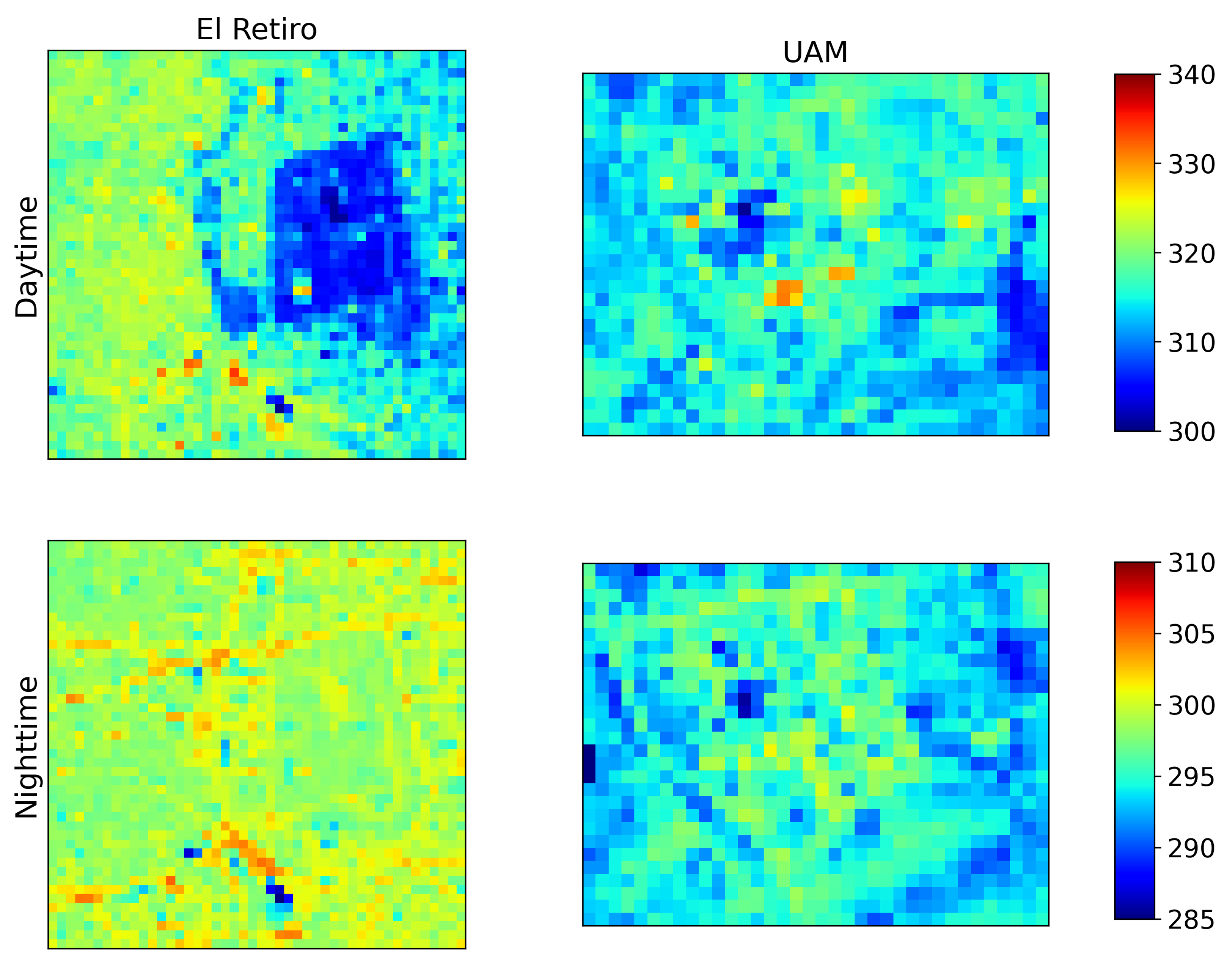
Figure 15 shows the retrieved LST over the Retiro and the UAM with the 1MMD-4-band TES at the satellite level and Table 10 shows their mean LST and standard deviations as well as the RMSE, MBE values between this LST and the aggregated LST from the same TES. This comparison allows highlighting the error due to the spatial resolution.
Visually, the Retiro park and its lake are discernible, as well as the denser historic neighborhood at the west of the park and the newer one at the north-east. In addition, during the nighttime, the main roads/streets are also distinguished. For the UAM, the same visual results as for Figure 13 are obtained: natural landscapes and roads can be observed. However, it is worth noting that the LST values overs roads or in the UAM campus cannot be seen due to the spatial resolution.
The RMSE values are 1.1 and 2.3 K for both areas during the daytime and nighttime. The MBE values are low during the daytime, with a value of −0.62 K for the Retiro Park and −0.34 K for the UAM. During the nighttime, the MBE values are higher, with −1.3 K for both study areas. The SSIM values are not high, 0.58 for the Retiro Park and 0.56 for the UAM, respectively, during the daytime, and −0.03 and −0.76 for the Retiro Park and the UAM, respectively, during the nighttime. The MBE values are negative, so the 60-m LST is lower than the aggregated one. In addition, the SSIM values are lower for the Retiro Park, due to the aggregation and the very dense spatial structure of the area. The first-order statistics are lower between the 1MMD-4-band TES and the aggregated LST map, the mean LST decreases by 0.5 and 1.3 K for the Retiro Park for daytime and nighttime, respectively. For the UAM, the mean decreases by 0.3 and 1.3 K for daytime and nighttime, respectively. The spatial variability of the LST is lower for the 1MMD-4-band TES than the aggregated map, meaning that the impact of the spatial resolution is noticeable on spatially averaged values, and the LST is smoothed.
Figure 16 shows the LST retrieved from the 2MMD-4-band TES at the satellite level for both Retiro and UAM areas and Table 8 provides their means and standard deviations, the RMSE, MBE and SSIM. Visually, the same observations as for the 1MMD-4-band TES can be made.
The RMSE values are between 1.25 and 2.5 K for both areas during the daytime and nighttime. The MBE values are −0.62 K for the Retiro Park and −0.42 K for the UAM for daytime. During the nighttime, the MBE values are higher, with −1.51 K for the Retiro Park and −1.61 K for the UAM. The SSIM values are not high, 0.59 for the Retiro Park and 0.56 for the UAM, respectively, during the daytime, −0.01 and 0.795 for the Retiro Park and the UAM, respectively, during the nighttime. The first-order statistics are lower for the 2MMD-4-band TES than the aggregated LST map. The mean LST decreases by 0.6 and 1.6 K for the Retiro Park for daytime and nighttime, respectively. For the UAM, the mean decreases by 0.4 and 1.4 K for daytime and nighttime, respectively. The LST spatial variability is not as high as with the aggregated map because of the lower values of the standard deviations. The impact of the spatial resolution is noticeable, the LST is smoothed (Table 11).
Lastly, Figure 17 shows the pixel per pixel difference between the 2MMD-4-band TES and the 1MMD-4-band TES. The same observations as in Figure 12 can be made. Indeed, during the daytime over the Retiro Park area, the pixel per pixel difference is positive over artificial surfaces between 0.5 and 1 K for daytime and almost 0.5 K for nighttime. The difference is negative over natural ones, between −0.5 and −1 K for daytime and nighttime, in agreement with the comparison at four meters for both airborne images and ground measurements. The difference is lower at nighttime than daytime for artificial materials, which is in agreement with their thermal inertia.

4.5. The SUHI Effect at 4 and 60 m

The SUHI is usually computed with mean LSTs at night [8,47]. Then, two areas are defined to compute the SUHI of Madrid from TRISHNA-like images, just like in [84]: an area around the Retiro park as the central urban zone and an area above the UAM area as the rural surroundings (see also Figure 2). Thus, Table 12 shows the SUHI values obtained both at 60-m and 4-m spatial resolutions, for the three dates (28 of June, 1 and 4 of July) and with the three TES methods studied in this work. The SUHI values of the 1MMD-4-band TES and 2MMD-4-band TES are very similar. The 1MMD-4-band TES and the 2MMD-4-band TES provide higher SUHI values than the 1MMD-7-band TES and at a 60-m spatial resolution, SUHI values are slightly higher than at a 4-m resolution, except for the 2MMD-4-band TES for two dates out of three. Moreover, some ground LST measurements made with four car transects at nighttime (22h just like the flight lines) give SUHI values shown in Table 12 [62]. The LST difference between urban and rural was measured at 22h00 for the four transects until the 3 of July. Then, Table 12 only shows the results of the LST difference for the 28 of June and the 1 of July. These values were collected in Appendix 1 of the ESA-DESIREX 2008 final report. It is worth noting that the areas of the four transects are not exactly the same as the ones used to compute the SUHI from remote data. However, the ground values are in good agreement with the SUHI remote values. The absolute value of difference between 4 and 60 m values is around 0.2 K for both 1MMD-4-band TES and 2MMD-4-band TES.
Figure 18 shows the SUHI map for the Retiro Park and the 4 of July at a 4-m spatial resolution and at a 60-m spatial resolution. For both spatial resolutions, the roads have the highest SUHI value. The average SUHI value for both spatial resolutions is between 6 and 7 K, in agreement with the results from Table 12. Both maps are very similar, but it can be observed at 60 m that the 2MMD-4-band TES has larger SUHI values than the 1MMD-4-band TES, especially for roads and the vegetated area of the Retiro Park due to the fact that the 2MMD-4-band TES is able to describe the high variability of LST, which strongly depends on the nature of the surfaces.

5. Discussion

5.1. Comparison between the 1-MMD-4-Band TES and the 2MMD-4-Band TES for LST and SUHI Retrieval

For LST retrieval, at four meters, the LST maps show that visually, there is a good agreement between the three versions of the TES algorithm and that there are physical patterns that can be explained. For instance, the left area of the Retiro Park is denser than the right one, leading to higher LSTs. It can also be due to the used building materials, as the left area is a historic neighborhood and the right one was built more recently. In addition, high LSTs are mainly found in streets, bare soil waste grounds and some buildings, with cooler areas prevailing in the vegetated areas around and some roofs. The same conclusions are obtained from the UAM area, buildings and bare soils, which present higher LSTs. During the day, the LST spatial variability is higher for the Retiro Park, which is explained by the larger amount of different materials in this area, whereas UAM is covered by a large part of natural surfaces that are similar (Figure 2 and Figure 3). Lastly, the spatial variability of the LST is lower at nighttime than daytime, explained by the absence of solar irradiance leading to the homogenization of the LST. Interestingly, some unusual physical patterns can be seen, especially over the Atocha train station where high and low LSTs are observed. It is mostly related to metals. Metallic materials are known to be poorly processed by the TES algorithm as the emissivity is very low and is considered as an outlier for the MMD relationship. Thus, the Atocha train station roof (south of the Retiro Park, see Figure 2) has a very low LST for both daytime and nighttime. This roof is classified as “roofs with metal” and “roofs with concrete”. It is possible to check visually on “Google Earth” images that this roof is an open car park with metal square-roofs. Thus, there is a strong cavity effect coupled with metal materials, which explains the unusual physical pattern. In addition, the center of the UAM area presents high LSTs and low LSTs. These patterns are not physical and can be due to errors in the LSE retrieval, the cavity effect or the no-exact-nadir-view of the AHS sensor. Newly, the roofs of the university are classified as “roofs with metal”. These roofs had a very low assigned emissivity in [63].
When comparing with ground LSTs, (Table 6, Table 7 and Table 8), the 2MMD-4-band TES outperforms the 1MMD-4-band TES over both natural and artificial materials. These results show the capacity of the double MMD relationship to recover a large variability of LST values, which become very important in urban environments where both natural and artificial materials are present. As expected, the largest discrepancies are seen for the artificial materials during the daytime. The ground LSTs are significantly higher than the retrieved LSTs, especially for the “CSIC” and “Urbanism” sites with a difference that can range from 14 to 17 K during the 4th of July, see Table 6. In addition, the RMSE value on daytime measures exceeds 7 K and it reaches 9 K for artificial materials. Even if the new 2MMD-4-band TES proposed in this study recovers a higher LST variability, it is still necessary to study it further in order to provide better results for very hot targets.
Other than the intrinsic limitations of TES to account for extreme LST values, these differences in LST when observing very hot targets can be due to several factors. First, at a very fine scale, the LST can be influenced by turbulences. Thus, if the measurements are not perfectly synchronized, temperature differences can appear and discrepancies increase as the ground sample distance is finer [85]. Looking at the ground measurements, the LST around the flight hour (10 min before and 10 min after) can vary from 1 to 3 K and even 10 K for the “CSIC” site during the daytime and from 0.5 to 1 K during the nighttime. Second, the pixels at the 4-m spatial resolution can be mixed. The retrieved LST is integrated over the pixel, which is of very different size than the punctual ground measurements. However, in this study, ground measurements have been performed on large enough homogeneous surfaces to neglect this effect.
Relatively to the LST maps, at a 4-m spatial resolution, the comparison with the 1MMD-7-band TES (used as a reference) gives a better RMSE value for the 2MMD-4-band TES but the MBE values are lower with the 1MMD-4-band TES, which can be explained by the fact that both the 1MMD-4-band TES and the 1MMD-7-band TES account for a lower LST variability than the 2MMD-4-band TES. In addition, the RMSE value difference between the 1MMD-4-band TES and the 1MMD-7-band TES can be due to the new urban-oriented MMD relationship that is better adapted to estimate LST on artificial materials but can overestimate the LST for natural materials, whereas the 1MMD-7-band TES tends to be optimal for the latter. Furthermore, MBE is a signed metric and so negative and positive errors can compensate leading to better values that are not exactly related to better local estimations. Figure 12 shows that the larger differences are seen over the artificial materials, which is in agreement with the ground LSTs.
At a 60-m spatial resolution, the pixel per pixel difference in Figure 17 shows that the larger differences are positive and are seen over the artificial materials, and they are negative over natural ones. Actually, the 60-m pixels are most of the time mixed pixels with a large number of materials inside. This reduces the performance of TES (independently of the number of MMD relationships) when recovering LST. However, the mixed nature of 60-m pixels does not strongly impact the classification step of the 2MMD-4-band TES since this classification only considers natural and artificial pixels. Nowadays, in the Madrid city center, the amount of natural surfaces in the urbanized area (out of parks) is negligible, and so to consider that pixels in the Retiro park are natural and pixels in urbanized neighborhoods are artificial is close to reality. Moreover, the size of the Retiro Park is greater than the pixel size, so a lot of pure natural-surface pixels are considered. The 1MMD-4-band TES tends to overestimate the natural materials, whereas the 2MMD-4-band TES is more adapted. Furthermore, the emissivity of a mixed pixel is not trivial to estimate so both methods tend to be less performant.
For SUHI retrieval, Figure 18, both methods provide similar patterns where the roads have the largest values. Compared with ground SUHI values, the 2MMD-4-band TES provides higher values than the 1MMD-4-band TES but both the methods provide close values. However, the 2MMD-4-band TES tends to provide the closest SUHI values to the 4-m maps than the 1MMD-4-band TES because the spatial LST variability is better retrieved, which is confirmed by the higher std values at 60 m for the 2MMD-4-band TES than with the 1MMD-4-band TES.
Given these observations, the 2MMD-4-band TES can be considered as a more optimal method to retrieve the SUHI value. Indeed, the use of other urban campaigns with airborne images and ground measurements will help to highlight the 2MMD-4-band TES contribution.

5.2. About the Use of a Ground Cover Classification Map

Considering the prevalence of the artificial materials in the urban areas and the comparison with ground LSTs showing better retrieval for these materials, the 2MMD-4-band TES is the most optimal method in this study by using an a priori about the land cover to help the TES algorithm to better process artificial and natural surfaces. However, the 2MMD-4-band TES requires a ground classification map with a satisfactory performance. Land cover retrieval still needs investigation and is not always available and the computation cost is higher, which can be prohibitory for a real-time process. TRISHNA will have concomitant reflective and thermal data so a near-similar classification process will be possible. However, TRISHNA will have only five multispectral bands in the reflective domain so the accuracy of the derived ground cover map can be lower than the ground cover used in this study, based on the 80 bands of AHS. This can be considered as a limitation but also shows the possibility of using no-sensor-related ground cover maps. It is worth noting that no optimal classification methods exist and are dependent on the available data. The ground classification map used in this study was also made thanks to ground measurements, and these latter observations are not always available. In addition, the comparison with ground LSTs showed that the 2MMD-4-band TES was not the optimal method for the bare soil site, whereas the 1MMD-7-band TES provides better results. This can be due to the higher number of bands used in the 1MMD-7-band TES. However, during the daytime, the difference is only 1 K between the 2MMD-4-band TES and the 1MMD-7-band TES, and during the nighttime, the difference is only 0.5 K. Moreover, this class contains only 3% of the pixels so this does not significantly impact the global results.
Lastly, a ground classification map can be less performant over mixed pixels according to the spatial structure and the spatial resolution because it considers pixels as pure. The results of this study show that the mixed pixels can be poorly processed by the TES algorithm independently of the number of MMD relationships.
Other land-cover-related products, such as the imperviousness, can be analyzed to replace the ground cover map.

5.3. TRISHNA Framework: Impact of the Spatial Resolution

The comparison of TRISHNA-like LST data with aggregated LST maps shows that the physical patterns are similar but that the spatial resolution impacts the performance of the TES for spatially averaged values. Some artificial structures are still discernible at a 60-m spatial resolution, especially roofs for the most part but also roads. The mean statistics of the LST show a satisfactory agreement between the 4-m spatial resolution and the 60-m one with a maximum difference of 2 K, due to the spatial smoothing. In addition, the observations show that the LST spatial variability decreases when the spatial resolution increases.
For the SUHI retrieval, the estimated values at the 60-m spatial resolution are in good agreement with the values at the 4-m spatial resolution with a difference of around 0.2 K. Figure 18 shows that for pure pixels, such as the vegetated area of the Retiro Park and its water lake, the spatial resolution does not strongly impact the SUHI values. On the contrary, the mixed pixels at 60 m have lower SUHI values, such as the roads with a difference of around 2 K between both spatial resolutions. Furthermore, the artificial materials provide higher SUHI values than natural ones, which is in agreement with the thermal inertia of the materials so a reliable analysis can be made.

6. Conclusions and Future Works

A new material-oriented TES algorithm has been developed through two new approaches: (i) the use of a more representative spectral database we called the urban-oriented database., which contains similar amounts of artificial materials and natural materials from laboratory or field spectra, (ii) the use of two MMD relationships instead of one by differentiating a MMD relationship for artificial materials (artificial-surface-oriented) and a MMD relationship for natural materials (natural-surface-oriented). An a priori under the form of a ground cover classification map is provided to the TES algorithm in order to choose the appropriate MMD relationship according to the land cover type.
The observations show: (1) the urban-oriented database is representative of the urban areas and allows to take into account artificial materials contrary to former classical databases. Using two databases instead of one allows preventing the overestimation of the LST over natural materials. (2) The 2MMD-4-band TES outperforms the two other versions of the TES made for comparison and validation when compared with ground LST measurements. (3) At a 4-m spatial resolution, in agreement with the ground LST measurements, the 2MMD-4-band TES outperforms the other TES algorithms over the artificial materials. (4) At a 60-m spatial resolution within the TRISHNA framework, observations show that the impact of the spatial resolution is observed by smoothing the LST, thus decreasing the LST spatial variability, especially for mixed pixels. Due to the spatial resolution, pure natural-surface-oriented pixels are more precisely processed by the 2MMD-4-band TES. (5) For the SUHI retrieval, the 2MMD-4-band TES is more optimal to retrieve the LST variability. As a conclusion, the 2MMD-4-band TES is the best algorithm for this study, considering only four bands instead of seven, which is a great result for multispectral sensors. The future TRISHNA sensor will provide observations allowing the monitoring of the LST and the SUHI effect.
Several ways of enhancement are identified: (1) Some studies about coupling TES and Split-Window (SW) algorithms have been conducted [86,87,88]. It can allow avoiding the emissivity a priori knowledge in the SW algorithm and the poor performance of the TES algorithm for low-spectral-contrast materials or metallic ones. The better knowledge of the impact of the 3D structure can lead to better LST retrievals especially for urban canyons [49], or the better knowledge of the adjacency effect [87]. Future works include the development of a hybridized TES algorithm to correct for both the spectral variability and the adjacency effect. (2) A ground cover classification map is not always available so other land-cover-related products should be investigated, such as the imperviousness. (3) Regarding the LSE retrieval to constrain the TES algorithm, multi-temporal acquisitions close in time or the link between visible indexes and thermal bands could improve the accuracy of this parameter [89]. (4) As the mean size of urban objects is less than the spatial resolution of the thermal satellite sensors, sharpening and unmixing procedures are necessary to be able to study the LST and the SUHI at finer scales [51,64,84,90,91,92]. (5) The use of other airborne campaigns such as ESA-THERMOPOLIS 2009 over Athens, Greece or AI4GEO/CAMCATT 2021 over Toulouse, France, with ground measurements is of great interest to pursue the study over urban areas [93]. Furthermore, the processing is only for a Mediterranean city in the south of Europe with low humidity profiles. Applications for other cities with different climates that include tropical zones would be of great interest as TRISHNA will also be dedicated to tropical regions.

Author Contributions

Conceptualization, A.M., C.G.-B. and X.B.; methodology, A.M., C.G.-B. and X.B.; software, A.M., C.G.-B., C.C., P.B. and L.P.; validation, C.G.-B.; formal analysis, A.M. and C.G.-B.; investigation, A.M., C.G.-B., C.C., P.B. and X.B.; resources, J.A.S.; data curation, A.M., C.G.-B., C.C. and P.B.; writing—original draft preparation, A.M., C.G.-B. and X.B.; writing—review and editing, A.M., C.G.-B., C.C., P.B., K.R.M.A., L.P., J.A.S. and X.B.; supervision, K.R.M.A. and X.B.; project administration, K.R.M.A. and X.B.; funding acquisition, X.B. and K.R.M.A. All authors have read and agreed to the published version of the manuscript.

Funding

This research was funded by CNES in the APR CATUT and APR AMISTAD frameworks. Data provided by the European Space Agency.

Institutional Review Board Statement

Not applicable.

Data Availability Statement

Data supporting the results are available upon reasonable request from the corresponding author.

Acknowledgments

The authors want to thank CNES for the granted projects, ESA and INTA for the ESA-DESIREX 2008 and AHS data and the anonymous reviewers for their relevant comments.

Conflicts of Interest

The authors declare no conflict of interest.

Abbreviations

The following abbreviations are used in this manuscript:
AHSAirborne Hyperspectral Scanner
APRAppel à Projets Recherches (Call for Research Proposal)
BOABottom of Atmosphere
CNESCentre National d’Etudes Spatiales (French Space Agency)
ESAEuropean Space Agency
FWHMFull Width at Half Maximum
INTAInstituto Nacional de Técnica Aeroespacial (Spanish Aerospace Institute)
ISROIndian Space Research Organization
LAILeaf Area Index
LSELand Surface Emissivity
LSTLand Surface Temperature
LSTMLand Surface Temperature Monitoring
MBEMean Bias Error
MMDMaximum Minimum Difference
NEMNormalized Emissivity Method
RMSERoot Mean Square Error
SAMSpectral Angle Mapper
SBGSurface Biology and Geology
SSIMStructural Similarity Index Measure
SUHISurface Urban Heat Island
SWSplit-Window
SWIRShortWave InfraRed
TESTemperature and Emissivity Separation
TIRThermal InfraRed
TOATop of Atmosphere
TRISHNAThermal infraRed Imaging Satellite for High-resolution Natural resource Assessment
UAMUniversidad Autónoma de Madrid
UHIUrban Heat Island
VNIRVisible and Near InfraRed

References

  1. United Nations. World Urbanization Prospects; Technical Report; United Nations: San Francisco, CA, USA, 2014. [Google Scholar]
  2. Zhao, L.; Oleson, K.; Bou-Zeid, E.; Krayenhoff, E.; Bray, A.; Zhu, Q.; Zheng, Z.; Chen, C.; Oppenheimer, M. Global Multi-Model Projections Of Local Urban Climates. Nat. Clim. Chang. 2021, 11, 152–157. [Google Scholar] [CrossRef]
  3. Mora, C.; Dousset, B.; Caldwell, I.R.; Powell, F.E.; Geronimo, R.C.; Bielecki, C.R.; Counsell, C.W.W.; Dietrich, B.S.; Johnston, E.T.; Louis, L.V.; et al. Global Risk Of Deadly Heat. Nat. Clim. Chang. 2017, 7, 501–506. [Google Scholar] [CrossRef]
  4. Hulley, M. 5—The Urban Heat Island Effect: Causes And Potential Solutions. In Metropolitan Sustainability; Woodhead Publishing Series in Energy; Woodhead Publishing: Sawston, UK, 2012; pp. 79–98. [Google Scholar]
  5. Nuruzzaman, M. Urban Heat Island: Causes, Effects and Mitigation Measures—A Review. Int. J. Environ. Monit. Anal. 2015, 3, 67–73. [Google Scholar] [CrossRef] [Green Version]
  6. Mohajerani, A.; Bakaric, J.; Jeffrey-Bailey, T. The Urban Meat Island Effect, Its causes, And Mitigation, With Teference To The Thermal Properties of Asphalt Concrete. J. Environ. Manag. 2017, 197, 522–538. [Google Scholar] [CrossRef] [PubMed]
  7. Prata, F.; Caselles, V.; Colland, C.; Sobrino, J.; Ottle, C. Thermal Remote Sensing of Land Surface Temperature From Satellites: Current Status and Future Prospects. Remote Sens. Rev. 1995, 12, 175–224. [Google Scholar] [CrossRef]
  8. Voogt, J.; Oke, T. Thermal Remote Sensing Of Urban Climates. Remote Sens. Environ. 2003, 86, 370–384. [Google Scholar] [CrossRef]
  9. Weng, Q. Thermal Infrared Remote Sensing For Urban Climate And Environmental Studies: Methods, Applications, And Trends. ISPRS J. Photogramm. Remote Sens. 2009, 64, 335–344. [Google Scholar] [CrossRef]
  10. Carrio, R.O. Thermal Remote Sensing of Urban Areas. The Case Study of the Urban Heat Island of Madrid. Ph.D. Thesis, Universitat de Valencia, Valencia, Spain, 2013. [Google Scholar]
  11. Parlow, E. Regarding Some Pitfalls in Urban Heat Island Studies Using Remote Sensing Technology. Remote Sens. 2021, 13, 3598. [Google Scholar] [CrossRef]
  12. Jones, P.; Jedlovec, G.; Suggs, R.; Haines, S. Using modis LST To Estimate Minimum Air Temperatures At Night. In Proceedings of the Conference on Satellite Meteorology and Oceanography, Norfolk, Virginian, 20–23 September 2004. [Google Scholar]
  13. Lele, S.; Chang, Y.; Sterner, R.; Glass, G. Integrating AVHRR Satellite Data And NOAA Ground Observations To Predict Surface Air Temperature: A Statistical Approach. Int. J. Remote Sens. 2004, 25, 2979–2994. [Google Scholar]
  14. Gallo, K.; Hale, R.; Tarpley, D.; Yu, Y. Evaluation of the Relationship between Air and Land Surface Temperature under Clear- and Cloudy-Sky Conditions. J. Appl. Meteorol. Climatol. 2011, 50, 767–775. [Google Scholar] [CrossRef]
  15. Schwarz, N.; Schlink, U.; Franck, U.; Großmann, K. Relationship Of Land Surface And Air Temperatures And Its Implications For Quantifying Urban Heat Island Indicators—An Application For The City Of Leipzig (Germany). Ecol. Indic. 2012, 18, 693–704. [Google Scholar] [CrossRef]
  16. Xu, Y.; Knudby, A.; Ho, H.C.D. Estimating Daily maximum Air Temperature From MODIS In British Columbia, Canada. Int. J. Remote Sens. 2014, 35, 8108–8121. [Google Scholar] [CrossRef]
  17. Kastendeuch, P.P.; Najjar, G.; Colin, J. Thermo-Radiative Simulation Of An Urban District With LASER/F. Urban Clim. 2017, 21, 43–65. [Google Scholar] [CrossRef]
  18. Masson, V.; Marchadier, C.; Adolphe, L.; Aguejdad, R.; Avner, P.; Bonhomme, M.; Bretagne, G.; Briottet, X.; Bueno, B.; de Munck, C.; et al. Adapting Cities To Climate Change: A Systemic Modelling Approach. Urban Clim. 2014, 10, 407–429. [Google Scholar] [CrossRef]
  19. Mitraka, Z.; Chrysoulakis, N. Earth Observation For Urban Climate Monitoring: Surface Cover And Land Surface Temperature; InTechOpen: London, UK, 2018. [Google Scholar]
  20. Jain, S.; Sannigrahi, S.; Sen, S.; Bhatt, S.; Chakraborti, S.; Rahmat, S. Urban Heat Island Intensity And Its Mitigation Strategies In The Fast-Growing Urban Area. J. Urban Manag. 2019, 9, 54–66. [Google Scholar] [CrossRef]
  21. Norman, J.M.; Becker, F. Terminology In Thermal Infrared Remote Sensing Of Natural Surfaces. Agric. For. Meteorol. 1995, 77, 153–166. [Google Scholar] [CrossRef]
  22. Bastiaanssen, W.; Pelgrum, H.; Wang, J.; Ma, Y.; Moreno, J.; Roerink, G.; van der Wal, T. A Remote Sensing Surface Energy Balance Algorithm For Land (SEBAL). J. Hydrol. 1998, 212, 213–229. [Google Scholar] [CrossRef]
  23. Kogan, F. Operational Space Technology For Global Vegetation Assessment. Bull. Am. Meteorol. Soc. 2001, 82, 1949–1964. [Google Scholar] [CrossRef]
  24. Su, B. The Surface Energy Balance System (SEBS) For Estimation Of Turbulent Heat Fluxes. Hydrol. Earth Syst. Sci. 2002, 6, 85–100. [Google Scholar] [CrossRef]
  25. Lagouarde, J.P.; Bhattacharya, B.; Crebassol, P.; Gamet, P.; Babu, S.; Boulet, G.; Briottet, X.; Buddhiraju, K.M.; Cherchali, S.; Dadou, I.; et al. The Indian-French Trishna Mission: Earth Observation in the Thermal Infrared With High Spatio-Temporal Resolution. In Proceedings of the IGARSS 2018—2018 IEEE International Geoscience and Remote Sensing Symposium 2018, Valencia, Spain, 22–27 July 2018; pp. 4078–4081. [Google Scholar]
  26. Lagouarde, J.P.; Bhattacharya, B.K.; Sarkar, S.S.; Boissin, B.; Crebassol, P.; Gamet, P. TRISHNA: A New High resolution Thermal Infrared Indo-French Mission Concept. In Proceedings of the International Symposium Recent Advances in Quantative Remote Sensing 2017, Valencia, Spain, 18–22 September 2017. [Google Scholar]
  27. Lagouarde, J.P.; Bach, M.; Sobrino, J.; Boulet, G.; Briottet, X.; Cherchali, S.; Coudert, B.; Dadou, I.; Dedieu, G.; Gamet, P.; et al. The MISTIGRI Thermal Infrared Project: Scientific Objectives And Mission Specifications. Int. J. Remote Sens. 2013, 34, 3437. [Google Scholar] [CrossRef]
  28. Crebassol, P.; Lagouarde, J.P.; Hook, S. Thirsty Thermal Infrared Spatial System. In Proceedings of the 2014 IEEE Geoscience and Remote Sensing Symposium, Quebec City, QC, Canada, 13–18 July 2014; pp. 3021–3024. [Google Scholar]
  29. Sobrino, J.; Oltra-Carrió, R.; Sòria, G.; Bianchi, R.; Paganini, M. Impact Of Spatial Resolution And Satellite Overpass Time On Evaluation Of The Surface Urban Heat Island Effects. Remote Sens. Environ. 2012, 117, 50–56. [Google Scholar] [CrossRef]
  30. Hulley, G.C.; Hook, S.J. HyspIRI Level-2 Thermal Infrared (TIR) Land Surface Temperature And Emissivity Algorithm Theoretical Basis Document; Jet Propulsion Laboratory, National Aeronautics and Space Administration: Pasadena, CA, USA, 2011. [Google Scholar]
  31. Roberts, D.A.; Quattrochi, D.A.; Hulley, G.C.; Hook, S.J.; Green, R.O. Synergies Between {VSWIR} and {TIR} Data for the Urban environment: An Evaluation of the Potential for the Hyperspectral Infrared Imager (HyspIRI) Decadal Survey mission. Remote Sens. Environ. 2012, 117, 83–101. [Google Scholar] [CrossRef]
  32. Chen, Y.; Duan, S.B.; Huazhong, R.; Labed, J.; Li, Z.L. Algorithm Development for Land Surface Temperature Retrieval: Application to Chinese Gaofen-5 Data. Remote Sens. 2017, 9, 161. [Google Scholar] [CrossRef] [Green Version]
  33. Koetz, B.; Bastiaanssen, W.; Berger, M.; Defourney, P.; Del Bello, U.; Drusch, M.; Drinkwater, M.; Duca, R.; Fernandez, V.; Ghent, D.; et al. High Spatio-Temporal Resolution Land Surface Temperature Mission—A Copernicus Candidate Mission In Support Of Agricultural Monitoring. In Proceedings of the IGARSS 2018—2018 IEEE International Geoscience and Remote Sensing Symposium, Valencia, Spain, 22–27 July 2018; pp. 8160–8162. [Google Scholar]
  34. Yang, Y.; Li, H.; Du, Y.; Cao, B.; Liu, Q.; Sun, L.; Zhu, J.; Mo, F. A Temperature And Emissivity Separation Algorithm For Chinese Gaofen-5 Satellite Data. In Proceedings of the IGARSS 2018—2018 IEEE International Geoscience and Remote Sensing Symposium, Valencia, Spain, 22–27 July 2018; pp. 2543–2546. [Google Scholar]
  35. National Academies of Sciences, Engineering, and Medicine. Thriving on Our Changing Planet: A Decadal Strategy for Earth Observation from Space; The National Academies Press: Washington, DC, USA, 2018. [Google Scholar]
  36. Gillespie, A.; Rokugawa, S.; Matsunaga, T.; Cothern, J.S.; Hook, S.; Kahle, A.B. A Temperature And Emissivity Separation Algorithm For Advanced Spaceborne Thermal Emission And Reflection Radiometer (ASTER) Images. IEEE Trans. Geosci. Remote Sens. 1998, 36, 1113–1126. [Google Scholar] [CrossRef]
  37. Sobrino, J.; Jimenez-Munoz, J.C. Land Surface Temperature Retrieval From Thermal Infrared Data: An Assessment In The Context Of The Surface Processes And Ecosystem Changes Through Response Analysis (SPECTRA) Mission. J. Geogr. Res. 2005, 110, D16103. [Google Scholar] [CrossRef] [Green Version]
  38. Sobrino, J.; Jimenez-Munoz, J.C.; Sòria Barres, G.; Gómez, M.; Ortiz, A.; Romaguera, M.; Julien, Y.; Cuenca, J.; Atitar, M.; Hidalgo, V.; et al. Thermal Remote Sensing In The Framework Of The SEN2FLEX Project: Field Measurements, Airborne Data And Applications. Int. J. Remote Sens. 2008, 29, 4961–4991. [Google Scholar] [CrossRef]
  39. Coll, C.; Garcia-Santos, V.; Niclòs, R.; Caselles, V. Test of the MODIS Land Surface Temperature and Emissivity Separation Algorithm With Ground Measurements Over A Rice Paddy. IEEE Trans. Geosci. Remote Sens. 2016, 54, 3061–3069. [Google Scholar] [CrossRef]
  40. Payan, V.; Royer, A. Analysis Of Temperature Emissivity Separation (TES) Algorithm Applicability And Sensitivity. Int. J. Remote Sens. 2004, 25, 15–37. [Google Scholar] [CrossRef]
  41. Gustafson, W.; Gillespie, A.; Yamada, G. Revisions to the ASTER Temperature/Emissivity Separation Algorithm. In Proceedings of the Second Recent Advances in Quantitative Remote Sensing, Torrent, Spain, 25–29 September 2006. [Google Scholar]
  42. Coll, C.; Caselles, V.; Valor, E.; Niclòs, R.; Sánchez, J.M.; Galve, J.M.; Mira, M. Temperature And Emissivity Separation From ASTER Data For Low Spectral Contrast Surfaces. Remote Sens. Environ. 2007, 110, 162–175. [Google Scholar] [CrossRef]
  43. Galve, J.; Coll, C.; Caselles, V.; Valor, E.; Mira, M. Comparison Of Split-Window And Single-Channel Methods For Land Surface Temperature Retrieval from MODIS and AATSR Data. In Proceedings of the IGARSS 2008—2008 IEEE International Geoscience and Remote Sensing Symposium 2008, Boston, MA, USA, 7–11 July 2008; Volume 3, pp. 294–297. [Google Scholar]
  44. Hulley, G.; Hughes, C.; Hook, S. Quantifying Uncertainties In Land Surface Temperature And Emissivity Retrievals From ASTER And MODIS Thermal Infrared Data. J. Geophys. Res. 2012, 117, 23113. [Google Scholar] [CrossRef] [Green Version]
  45. Mohamed, A.A.; Odindi, J.; Mutanga, O. Land Surface Temperature And Emissivity Estimation For Urban Heat Island Assessment Using Medium- And Low-Resolution Space-borne Sensors: A review. Geocarto Int. 2017, 32, 455–470. [Google Scholar] [CrossRef]
  46. Mullerova, D.; Williams, M. Satellite Monitoring Of Thermal Performance in Smart Urban Designs. Remote Sens. 2019, 11, 2244. [Google Scholar] [CrossRef] [Green Version]
  47. Sobrino, J.; Oltra-Carrió, R.; Sòria Barres, G.; Jimenez-Munoz, J.C.; Franch, B.; Hidalgo, V.; Mattar, C.; Julien, Y.; Cuenca, J.; Romaguera, M.; et al. Evaluation Of The Surface Urban Heat Island Effect In The City Of Madrid By Thermal Remote Sensing. Int. J. Remote Sens. 2013, 34, 3177. [Google Scholar] [CrossRef]
  48. Fontanilles, G.; Briottet, X.; Fabre, S.; Trémas, T.; Henry, P. TITAN: A New Infrared Radiative Transfer model For The Study Of Heterogeneous 3D Surface. In Proceedings of the SPIE—The International Society for Optical Engineering, Wales, UK, 5–17 September 2008; Volume 7107. [Google Scholar]
  49. Roupioz, L.; Nerry, F.; Colin, J. Correction For The Impact Of The Surface Characteristics On The Estimation Of The Effective Emissivity At Fine Resolution In Urban Areas. Remote Sens. 2018, 10, 746. [Google Scholar] [CrossRef] [Green Version]
  50. Small, C. Multiresolution analysis of urban reflectance. In Proceedings of the IEEE/ISPRS Joint Workshop on Remote Sensing and Data Fusion over Urban Areas, Rome, Italy, 8–9 November 2001; pp. 15–19. [Google Scholar]
  51. Mechri, R. Désagrégation Spatiale de Températures Météosat par une Méthode d’Assimilation de Données (Lisseur Particulaire) Dans un Modèle de Surface Continentale. Ph.D. Thesis, Versailles Saint-Quentin-en-Yvelines University, Versailles, France, 2014. [Google Scholar]
  52. Granero-Belinchon, C.; Michel, A.; Achard, V.; Briottet, X. Spectral Unmixing For Thermal Infrared Multi-spectral Airborne Imagery Over Urban Environments: Day and Night Synergy. Remote Sens. 2020, 12, 1871. [Google Scholar] [CrossRef]
  53. Zheng, X.; Li, Z.L.; Zhang, X.; Shang, G. Quantification Of The Adjacency Effect On Measurements In The Thermal Infrared Region. IEEE Trans. Geosci. Remote Sens. 2019, 57, 9674–9687. [Google Scholar] [CrossRef]
  54. Lagouarde, J.P.; Irvine, M. Directional Anisotropy In Thermal Infrared Measurements Over Toulouse City Centre During the CAPITOUL Measurement Campaigns: First Results. Meteorol. Atmos. Phys. 2008, 102, 173–185. [Google Scholar] [CrossRef]
  55. Ben-Dor, E.; Levin, N.; Saaroni, H. A Spectral Based Recognition Of The Urban Environment Using The Visible And Near-Infrared Spectral Region (0.4–1.1 m). A Case Study Over Tel-Aviv, Israel. Int. J. Remote Sens. 2001, 22, 2193–2218. [Google Scholar]
  56. Roberts, D.; Herold, M. Imaging Spectrometry of Urban Materials. Infrared Spectrosc. Geochem. Explor. Remote Sens. Miner. Assoc. Can. Short Course Ser. 2004, 33, 155–181. [Google Scholar]
  57. Cadenasso, M.L.; Pickett, S.T.A.; Schwarz, K. Spatial Heterogeneity in Urban Ecosystems: Reconceptualizing Land Cover and a Framework for Classification. Front. Ecol. Environ. 2007, 5, 80–88. [Google Scholar] [CrossRef]
  58. Greinert, A. The Heterogeneity Of Urban Soils In The Light Of Their Properties. J. Soils Sediments 2015, 15, 1725–1737. [Google Scholar] [CrossRef] [Green Version]
  59. Oltra-Carrió, R.; Sobrino, J.; Franch, B.; Nerry, F. Land Surface Emissivity Retrieval From Airborne Sensor Over Urban Areas. Remote Sens. Environ. 2012, 123, 298–305. [Google Scholar] [CrossRef]
  60. Pérez-Planells, L.; Valor, E.; Coll, C.; Niclòs, R. Comparison and Evaluation of the TES and ANEM Algorithms for Land Surface Temperature and Emissivity Separation over the Area of Valencia, Spain. Remote Sens. 2017, 9, 1251. [Google Scholar] [CrossRef] [Green Version]
  61. Sobrino, J.A.; Jiménez-Muñoz, J.C.; Zarco-Tejada, P.J.; Sepulcre-Cantó, G.; de Miguel, E. Land Surface Temperature Derived From Airborne Hyperspectral scanner Thermal Infrared Data. Remote Sens. Environ. 2006, 102, 99–115. [Google Scholar] [CrossRef]
  62. Sobrino, J.; Sòria, G.; Oltra-Carrió, R.; Noz, J.J.M.; Romaguera, M.; Cuenca, J.; Hidalgo, V.; Franch, B.; Mattar, C.; Julien, Y.; et al. DESIREX 2008 Final Report; Technical Report; 2009; Available online: https://www.researchgate.net/publication/315814196_Dual-use_European_Security_IR_Experiment_2008_DESIREX_2008_FINAL_REPORT (accessed on 12 October 2021).
  63. Sobrino, J.A.; Oltra-Carrió, R.; Jiménez-Muñoz, J.C.; Julien, Y.; Sòria, G.; Franch, B.; Mattar, C. Emissivity Mapping Over Urban Areas Using A Classification-Based Approach: Application To The Dual-use European Security IR Experiment (DESIREX). Int. J. Appl. Earth Obs. Geoinf. 2012, 18, 141–147. [Google Scholar] [CrossRef]
  64. Granero-Belinchon, C.; Michel, A.; Lagouarde, J.P.; Sobrino, J.; Briottet, X. Multi-Resolution Study of Thermal Unmixing Techniques Over Madrid Urban Area: Case Study Of TRISHNA Mission. Remote Sens. 2019, 11, 1251. [Google Scholar] [CrossRef] [Green Version]
  65. Poutier, L.; Miesch, C.; Lenot, X.; Achard, V.; Boucher, Y. COMANCHE And COCHISE: Two Reciprocal Atmospheric Codes For Hyperspectral Remote Sensing. In Proceedings of the 2002 AVIRIS Earth Science and Applications Workshop Proceedings, Pasadena, CA, USA, 5–8 March 2002. [Google Scholar]
  66. Miesch, C.; Poutier, L.; Achard, V.; Briottet, X.; Lenot, X.; Boucher, Y. Direct And Inverse Radiative Transfer Solutions For Visible And Near-Infrared Hyperspectral Imagery. IEEE Trans. Geosci. Remote Sens. 2005, 43, 1552–1562. [Google Scholar] [CrossRef]
  67. Baldridge, A.; Hook, S.; Grove, C.; Rivera, G. The ASTER Spectral Library Version 2.0. Remote Sens. Environ. 2009, 113, 711–715. [Google Scholar] [CrossRef]
  68. Meerdink, S.; Hook, S.; Roberts, D.; Abbott, E. The ECOSTRESS Spectral Library Sersion 1.0. Remote Sens. Environ. 2019, 230, 111196. [Google Scholar] [CrossRef]
  69. Masson, V.; Gomes, L.; Pigeon, G.; Liousse, C.; Pont, V.; Lagouarde, J.P.; Voogt, J.; Salmond, J.; Oke, T.R.; Hidalgo, J.; et al. The Canopy and Aerosol Particles Interactions in TOulouse Urban Layer (CAPITOUL) Experiment. Meteorol. Atmos. Phys. 2008, 102, 135. [Google Scholar] [CrossRef]
  70. Kotthaus, S.; Smith, T.E.; Wooster, M.J.; Grimmond, C. Derivation Of An Urban Materials Spectral Library Through Emittance And Reflectance Spectroscopy. ISPRS J. Photogramm. Remote Sens. 2014, 94, 194–212. [Google Scholar] [CrossRef] [Green Version]
  71. Snyder, W.C.; Wan, Z.; Zhang, Y.; Feng, Y.Z. Thermal Infrared (3–14 μm) Bidirectional Reflectance Measurements Of Sands And Soils. Remote Sens. Environ. 1997, 60, 101–109. [Google Scholar] [CrossRef]
  72. Gerber, F.; Marion, R.; Olioso, A.; Jacquemoud, S.; Ribeiro Da Luz, B.; Fabre, S. Modeling Directional-Hemispherical Reflectance and Transmittance Of Fresh And Dry Leaves From 0.4 μm to 5.7 μm With The PROSPECT-VISIR Model. Remote Sens. Environ. 2011, 115, 404–414. [Google Scholar] [CrossRef]
  73. Lesaignoux, A.; Jacob, F.; Olioso, A.; Weiss, M.; Nerry, F.; Sobrino, J.; Gamet, P.; Jacquemoud, S.; Caillault, K.; Labarre, L.; et al. Spécification Des Bandes Spectrales Infrarouges Thermiques De L’Instrument MISTIGRI: Développement Du Simulateur De La Mesure (SiMi), Restitution Des Variables D’intéret Par Inversion Du Transfert Radiatif, Identification De La Configuration Spectrale Optimale; Technical Report; IRD: Wellington, New Zealand, 2014. [Google Scholar]
  74. Jacob, F.; Lesaignoux, A.; Olioso, A.; Weiss, M.; Caillault, K.; Jacquemoud, S.; Nerry, F.; French, A.; Schmugge, T.; Briottet, X.; et al. Reassessment Of The Temperature-Emissivity Separation From Multispectral Thermal Infrared data: Introducing The impact Of Vegetation Canopy By Simulating The Cavity Effect With The SAIL-Thermique model. Remote Sens. Environ. 2017, 198, 160–172. [Google Scholar] [CrossRef]
  75. Lesaignoux, A.; Fabre, S.; Briottet, X. Influence Of Soil Moisture Content On Spectral Reflectance Of Bare Soils In The 0.4–14 μm Domain. Int. J. Remote Sens. 2013, 34, 2268–2285. [Google Scholar] [CrossRef]
  76. Girouard, G.S.; Bannari, A.; Harti, A.; Desrochers, A. Validated Spectral Angle Mapper Algorithm for Geological Mapping: Comparative Study Between Quickbird And Landsat-TM. In Proceedings of the XXth ISPRS congress, geo-imagery bridging continents, Istanbul, Turkey, 12–23 July 2004. [Google Scholar]
  77. Verhoef, W. Light Scattering By Leaf Layers With Application To Canopy Reflectance Modeling: The SAIL Model. Remote Sens. Environ. 1984, 16, 125–141. [Google Scholar] [CrossRef] [Green Version]
  78. Oltra-Carrió, R.; Cubero-Castan, M.; Briottet, X.; Sobrino, J.A. Analysis Of The Performance of the TES Algorithm Over Urban Areas. IEEE Trans. Geosci. Remote Sens. 2014, 52, 6989–6998. [Google Scholar] [CrossRef] [Green Version]
  79. Kerr, Y.H.; Lagouarde, J.; Nerry, F.; Ottle, C. Land Surface Temperature Retrieval Techniques and Applications. In Thermal Remote Sensing in Land Surface Processes; CRC Press: Boca Raton, FL, USA, 2000. [Google Scholar]
  80. Li, Z.L.; Tang, B.H.; Wu, H.; Ren, H.; Yan, G.; Wan, Z.; Trigo, I.F.; Sobrino, J.A. Satellite-Derived Land Surface Temperature: Current Status and Perspectives. Remote Sens. Environ. 2013, 131, 14–37. [Google Scholar] [CrossRef] [Green Version]
  81. Dash, P.; Göttsche, F.M.; Olesen, F.; Fischer, H. Land Surface Temperature and Emissivity Estimation from Passive Sensor Data: Theory and Practice-Current Trends. Int. J. Remote Sens. 2002, 23, 2563. [Google Scholar] [CrossRef]
  82. Hulley, G.C.; Ghent, D.; Göttsche, F.M.; Guillevic, P.C.; Mildrexler, D.J.; Coll, C. 3—Land Surface Temperature. In Taking the Temperature of the Earth; Hulley, G.C., Ghent, D., Eds.; Elsevier: Amsterdam, The Netherlands, 2019; pp. 57–127. [Google Scholar] [CrossRef]
  83. Gillespie, A.R.; Rokugawa, S.; Hook, S.J.; Matsunaga, T.; Kahle, A.B. Temperature/Emissivity Separation Algorithm Theoretical Basis Document, Version 2.4; NASA: Washington, DC, USA, 1999. [Google Scholar]
  84. Granero-Belinchon, C.; Michel, A.; Lagouarde, J.P.; Sobrino, J.; Briottet, X. Night Thermal Unmixing For The Study Of Microscale Surface Urban Heat Islands With TRISHNA-Like Data. Remote Sens. 2019, 11, 1449. [Google Scholar] [CrossRef] [Green Version]
  85. Lagouarde, J.P.; Irvine, M.; Dupont, S. Atmospheric Turbulence Induced Errors On Measurements Of Surface Temperature From Space. Remote Sens. Environ. 2015, 168, 40–53. [Google Scholar] [CrossRef]
  86. Huazhong, R.; Ye, X.; Liu, R.; Dong, J.; Qin, Q. Improving Land Surface Temperature And Emissivity Retrieval From The Chinese Gaofen-5 Satellite Using A Hybrid Algorithm. IEEE Trans. Geosci. Remote Sens. 2017, 56, 1080–1090. [Google Scholar]
  87. Zheng, X.; Li, Z.; Nerry, F.; Zhang, X. A New Thermal Infrared Channel Configuration For Accurate Land Surface Temperature Retrieval From Satellite Data. Remote Sens. Environ. 2019, 231, 111216. [Google Scholar] [CrossRef]
  88. Ren, H.; Dong, J.; Liu, R.; Zheng, Y.; Guo, J.; Chen, S.; Nie, J.; Zhao, Y. New Hybrid Algorithm For Land Surface Temperature Retrieval From Multiple-Band Thermal Infrared Image Without Atmospheric And Emissivity Data Inputs. Int. J. Digit. Earth 2020, 13, 1430–1453. [Google Scholar] [CrossRef]
  89. Olioso, A.; Briottet, X.; Fabre, S.; Jacob, F.; Michel, A.; Nativel, S.; Rivalland, V.; Roujean, J. Relations Between Landsat Spectral Reflectances And Land Surface Emissivity Over Bare Soils. In Proceedings of the IGARSS 2019—2019 IEEE International Geoscience and Remote Sensing Symposium, Yokohama, Japan, 28 July–2 August 2019; pp. 6937–6940. [Google Scholar]
  90. Mechri, R.; Ottlé, C.; Pannekoucke, O.; Kallel, A.; Maignan, F.; Courault, D.; Trigo, I.F. Downscaling Meteosat Land Surface Temperature Over a Heterogeneous Landscape Using a Data Assimilation Approach. Remote Sens. 2016, 8, 586. [Google Scholar] [CrossRef] [Green Version]
  91. Cubero-Castan, M.; Chanussot, J.; Achard, V.; Briottet, X.; Shimoni, M. A Physics-Based Unmixing Method To Estimate Subpixel Temperatures On Mixed Pixels. IEEE Trans. Geosci. Remote Sens. 2015, 53, 1894–1906. [Google Scholar] [CrossRef]
  92. Li, W.; Ni, L.; Wu, H.; Li, Z.L.; Duan, S.B. Evaluation of Machine Learning Algorithms in Spatial Downscaling of MODIS Land Surface Temperature. IEEE J. Sel. Top. Appl. Earth Obs. Remote Sens. 2019, 12, 2299–2307. [Google Scholar] [CrossRef]
  93. Daglis, I.; Rapsomanikis, S.; Kourtidis, K.; Melas, D.; Keramitsoglou, I.; Giannaros, T.; Amiridis, V.; Sobrino, J.; Manunta, P.; Grobner, J.; et al. Results Of The Thermopolis 2009 Campaign With Regard To The Urban Heat Island (UHI) Effect In Athens. In Proceedings of the ESA Living Planet Symposium, Bergen, Norway, 28 June–2 July 2010. [Google Scholar]
Figure 1. RGB AHS image for the 4 of July of 2008. Yellow squares highlight the two areas used for visual analysis: the Retiro Park in the center of Madrid and the Universidad Autonoma de Madrid (UAM) in the peri-urban northern area of the city. North is marked by the arrow. The green square highlights the rural area, and the purple square highlights the urban area; both areas were chosen to compute the SUHI. Green stars point out the locations of ground measurements from calibration/validation sites or from fixed masts, with numbers in correspondence with Table 2.
Remotesensing 13 05139 g001
Figure 2. RGB AHS image for the 4 of July 2008 over the two areas shown for visual analysis: the Retiro Park (left) and the UAM (right). Stars point out the calibration and validation surfaces used during the ESA-DESIREX campaign, with numbers in correspondence with Table 2. The water lake is at the center of the Retiro Park, highlighted by the number three. The big gray roofs under the Retiro Park are part of the Atocha train station.
Remotesensing 13 05139 g002
Figure 3. The 4-m classification map derived from AHS and in-situ data, over the Retiro Park (top left), over the UAM (top right), with the legend and the density of each class in percentage (bottom).
Remotesensing 13 05139 g003
Figure 4. Processing scheme from AHS data to TRISHNA data in the TIR.
Remotesensing 13 05139 g004
Figure 5. Illustration of the methodology applied on one thermal band (72) over the Retiro Park (up) and the UAM (bottom): before Step 1 (left), after Step 1 (middle), after Step 2 (right).
Remotesensing 13 05139 g005
Figure 6. The 60-m classification map obtained from the 4-m one over the Retiro Park (top left) and the UAM (top right), with the legend and the density of each class in percentage (bottom).
Remotesensing 13 05139 g006
Figure 7. MMD relationship statistical fits for the 1MMD TES with the urban-oriented database: calibration (left) and validation (right). The obtained MMD relationship is highlighted with a red line.
Remotesensing 13 05139 g007
Figure 8. MMD relationship statistical fits for the 2MMD TES: artificial-surface-oriented database (up), natural-surface-oriented database (bottom) calibration (left), validation (right). The obtained MMD relationship is higlighted with a red line.
Remotesensing 13 05139 g008
Figure 9. LST in K retrieved from the 1MMD-7-band TES of [59] over the Retiro park daytime (top left) and nighttime (bottom left) and over the UAM area daytime (top right) and nighttime (bottom right).
Remotesensing 13 05139 g009
Figure 10. LST in K retrieved from the hlm1MMD-4-band TES over the Retiro Park (left) and the UAM (right) during the daytime (top) and nighttime (bottom).
Remotesensing 13 05139 g010
Figure 11. LST in K retrieved from the 2MMD-4-band TES over the Retiro Park (left) and the UAM (right) during the daytime (top) and nighttime (bottom).
Remotesensing 13 05139 g011
Figure 12. Pixel per pixel difference of the LST in K between the 2MMD-4-band TES and the 1MMD-4-band TES over the Retiro Park (left) and the UAM (right) during the daytime (top) and nighttime (bottom).
Remotesensing 13 05139 g012
Figure 13. The 60-m aggregated LST from the 1MMD-4-band TES over the Retiro park (left) and the UAM (right) during the daytime (top) and nighttime (bottom).
Remotesensing 13 05139 g013
Figure 14. The 60-m aggregated LST from the 2MMD-4-band TES over the Retiro park (left) and the UAM (right) during the daytime (top) and nighttime (bottom).
Remotesensing 13 05139 g014
Figure 15. LST in K retrieved from the 1MMD-4-band TES over the Retiro Park (left) and the UAM (right) during the daytime (top) and nighttime (bottom).
Remotesensing 13 05139 g015
Figure 16. LST in K retrieved from the 2MMD-4-band TES over the Retiro Park (left) and the UAM (right) during the daytime (top) and nighttime (bottom).
Remotesensing 13 05139 g016
Figure 17. Pixel per pixel difference of the LST in K between the 2MMD-4-band TES and the 1MMD-4-band TES over the Retiro Park (left) and the UAM (right) during the daytime (top) and nighttime (bottom).
Remotesensing 13 05139 g017
Figure 18. SUHI in K retrieved over the Retiro Park with the 1MMD-4-band TES (left) and the 2MMD-4-band TES (right) at a 4-m spatial resolution (top), at a 60-m spatial resolution (bottom).
Remotesensing 13 05139 g018
Table 1. Effective wavelength and FWHM of the different AHS spectral thermal bands.
AHS Band71727374757677787980
Effective wavelength ( μ m)8.188.669.159.610.0710.5911.1811.7812.3512.93
FWHM (nm)370390410430420550560560480490
Table 2. Names and locations of the calibration/validation sites and fixed masts.
SiteCoordinates: Latitude, Longitude
1/ Fixed Mast and Calibration/Validation: rugby field UAM (natural material)40°32 50.58 N, 3°41 53.57 W
2/ Calibration/Validation: soccer field UAM (natural material)40°32 52.37 N, 3°41 48.08″ W
3/ Calibration/Validation: water lake Retiro Park (natural material)40°25 1.70 N, 3°41′2.27″ W
4/ Fixed mast: CSIC (artificial material)40°26 28.06 N, 3°41 15.54 W
5/ Fixed mast: Printing (artificial material)40°24 49.96 N, 3°42 19.87 W
6/ Fixed mast: Urbanism Building (artificial material)40°27 36.31 N, 3°40 19.86 W
Table 3. Coefficients a, b and c for the MMD relationship according to the database and the number of bands.
TES Algorithmabc
1MMD-4-band TES and urban-oriented database0.975−0.9060.953
1MMD-7-band TES and classical database [10]0.999−0.7770.815
2MMD-4-band TES and natural-surface-oriented database0.982−0.7950.915
2MMD-4-band TES and artificial-surface-oriented database0.960−1.0281.055
Table 4. First-order statistics of the 1MMD-7-band TES over the Retiro park and the UAM areas for the 4 of July 2008.
AreaMean (K)Std (K)
daytimeRetiro park315.88.7
UAM314.26.4
nighttimeRetiro park298.53.2
UAM294.13.2
Table 5. RMSE, MBE and SSIM between 7-band TES from [59] and 1MMD-TES and 2MMD-TES, respectively. First-order statistics of the 1MMD-TES and 2MMD-TES over the Retiro park and the UAM areas are also shown. Date: 4 of July 2008.
AreaRMSE (K)MBE (K)SSIMMean (K)Std (K)
1MMD-TESdaytimeRetiro park1.13−0.770.98316.68.7
UAM0.68−0.560.98314.96.2
nighttimeRetiro park1.12−0.390.92298.93.7
UAM0.80−0.240.83294.43.3
2MMD-TESdaytimeRetiro park0.91−0.930.98316.88.7
UAM0.62−0.720.98315.06.3
nighttimeRetiro park0.95−0.570.93299.13.6
UAM1.07−0.380.85294.53.5
Table 6. LST values for each method and the ground LSTs for the 4 of July 2008 during the daytime. * indicates the retrieved LST closest to the ground measurement.
LocationGround LST (K)1MMD-7-Band TES LST (K)1MMD-4-Band TES LST (K)2MMD-4-Band TES LST (K)
4/ CSIC (roof)336.4329.6331.8332.6 *
5/ Printing (roof)339.2323.7325.2325.8 *
6/ Urbanism (roof)340.4321.1322.6323.1 *
1/ Rugby field (green grass)302.9307.6 *308.9308.4
2/ Soccer field (bare soil)313.7314.4 *314.7315.4
3/ Retiro lake (water)300.5300.0301.1300.7 *
Table 7. LST values for each method and the ground LSTs the 4 of July 2008 during the nighttime. * indicates the retrieved LST closest to the ground measurement.
LocationGround LST (K)1MMD-7-Band TES LST (K)1MMD-4-Band TES LST (K)2MMD-4-Band TES LST (K)
CSIC (roof)302.8297.8298.7299.3 *
Printing (roof)302.8297.1297.5298.0 *
Urbanism (roof)298.5298.2298.1298.6 *
Rugby field UAM (green grass)288.7288.3289.1288.7 *
Soccer field UAM (bare soil)295.8295.7 *294.4295.2
Retiro Park lake (water)299.9301.1300.7
Table 8. RMSE, MBE between the retrieved LSTs for each method and the ground LSTs combining all the six available flightlines. * indicates the lowest RMSE value.
MethodRMSE (K)MBE (K)
1MMD-4-band TES daytime8.3−3.0
2MMD-4-band TES daytime7.9 *−2.9 *
1MMD-7-band TES daytime9.0−4.1
1MMD-4-band TES nighttime3.5−2.6
2MMD-4-band TES nighttime3.2 *−2.2 *
1MMD-7-band TES nighttime4.0−2.9
1MMD-4-band TES artificial9.5−7.7
2MMD-4-band TES artificial9.0 *−7.1 *
1MMD-7-band TES artificial10.6−8.8
1MMD-4-band TES natural3.01.0
2MMD-4-band TES natural2.81.0
1MMD-7-band TES natural2.6 *0.5 *
1MMD-4-band TES global6.7−2.8
2MMD-4-band TES global6.3 *−2.6 *
1MMD-7-band TES global7.3−3.6
Table 9. First-order statistics for the aggregated LST maps according to each method.
Mean (K)Std (K)Mean (K)Std (K)
Area2MMD-4-Band TES2MMD-4-Band TES1MMD-4-Band TES1MMD-4-Band TES
daytimeRetiro park317.26.0316.85.7
UAM315.13.8314.93.6
nighttimeRetiro park299.31.8299.01.8
UAM294.52.4294.42.2
Table 10. RMSE, MBE and SSIM between the 60-m LST from the 1MMD-4-band TES and the aggregated 4-m to 60-m LST from the 1MMD-4-band TES and 1st-order statistics of the former.
AreaRMSE (K)MBE (K)SSIMMean (K)Std (K)
daytimeRetiro park2.32−0.540.58316.35.2
UAM2.33−0.320.56314.62.7
nighttimeRetiro park2.04−1.30−0.03297.71.2
UAM1.13−1.340.76293.11.8
Table 11. RMSE, MBE and SSIM between the the 60-m LST from the 2MMD-4-band TES and the 60-m aggregated LST from the 2MMD-4-band TES and 1st-order statistics of the former.
AreaRMSE (K)MBE (K)SSIMMean (K)Std (K)
daytimeRetiro park2.41−0.620.59316.65.5
UAM2.46−0.420.56314.72.95
nighttimeRetiro park2.08−1.51−0.01297.81.3
UAM1.25−1.610.75292.92.05
Table 12. Estimated SUHI from 60-m and 4-m LST with the 1MMD-7-band TES, 1MMD-4-band TES and 2MMD-4-band TES, and from ground measurements of LST. Results for the three studied dates are shown.
Spatial ResolutionLST Retrieval Methodology28 June1 July4 July
60 m1MMD-4-band TES (K)9.579.567.02
2MMD-4-band TES (K)9.589.587.45
4 m1MMD-7-band TES (K)9.219.156.59
1MMD-4-band TES (K)9.359.306.79
2MMD-4-band TES (K)9.809.777.21
In situCar transect 1 (K)9.109.7x
Car transect 2 (K)9.57.7x
Car transect 3 (K)7.98.8x
Car transect 4 (K)9.311.4x
Publisher’s Note: MDPI stays neutral with regard to jurisdictional claims in published maps and institutional affiliations.

