Abstract
Oxytropis ochrocephala Bunge is an herbaceous perennial poisonous weed. It severely affects the production of local animal husbandry and ecosystem stability in the source region of Yellow River (SRYR), China. To date, however, the spatiotemporal distribution of O. ochrocephala is still unclear, mainly due to lack of high-precision observation data and effective methods at a regional scale. In this study, an efficient sampling method, based on unmanned aerial vehicle (UAV), was proposed to supply basic sampling data for species distribution models (SDMs, BIOMOD in this study). A total of 3232 aerial photographs were obtained, from 2018 to 2020, in SRYR, and the potential and future distribution of O. ochrocephala were predicted by an ensemble model, consisting of six basic models of BIOMOD. The results showed that: (1) O. ochrocephala mainly distributed in the southwest, middle, and northeast of the SRYR, and the high suitable habitat of O. ochrocephala accounted for 3.19%; (2) annual precipitation and annual mean temperature were the two most important factors that affect the distribution of O. ochrocephala, with a cumulative importance of 60.45%; and (3) the distribution probability of O. ochrocephala tends to increase from now to the 2070s, while spatial distribution ranges will remain in the southwest, middle, and northeast of the SRYR. This study shows that UAVs can potentially be used to obtain the basic data for species distribution modeling; the results are both beneficial to establishing reasonable management practices and animal husbandry in alpine grassland systems.
1. Introduction
Global climate change has caused substantial changes to the natural environment [1] and, therefore, became the dominant environmental factor affecting the geographical distribution of species [2], especially in the high-altitude regions. The source region of the Yellow River (SRYR), located in the northeast edge of the Qinghai–Tibetan Plateau (QTP, China), is an important water conservation area and ecological security barrier [3], and one of the most important animal husbandry industrial bases of China [4]. As the main carrier of natural resources and ecological environment [5,6], alpine meadows account for about 80% of the total area of the SRYR. Climate change, irrational human activities, and management are primarily responsible for the continuous deterioration of plant community structure, including the fast spread of poisonous weeds [7]. It is found that the sustainable development of the ecological environment and animal husbandry in the SRYR has been seriously threatened by poisonous weeds [7,8]. One of the most important undesirable species on QTP is Oxytropis ochrocephala Bunge, an herbaceous perennial poisonous weed that is rich in indolizine alkaloid (swainsonine) [9]. It may cause livestock poisoning directly and affect their growth, reproduction, and breed improvement indirectly, especially in the areas suffering long-term overgrazing [10]. In addition, O. ochrocephala could induce a strong allelopathy during the process of decomposition [11], which may inhibit forage growth, reduce species diversity, aggravate grassland degradation, and even destroy the ecological balance of grassland [12]. However, as a significant source of nitrogen in a natural grassland, the nitrogen fixation of O. ochrocephala is beneficial to the alpine grassland ecosystem development [13]; thus, it could play a positive role if reasonably managed. To date, the distribution of O. ochrocephala, and its relationship to relevant geographical environment variables, are poorly known. This study is the first attempt to depict the spatiotemporal distribution of O. ochrocephala, especially, predicting its suitable habitat distribution and response to climate change.
Species distribution modeling (SDMs) is essential to ensure the consistency of large-scale studies of biodiversity [14,15], particularly in the fields of invasive, conservation and evolutionary biology, and biogeography [16]. SDMs can fit very complex relationships between species presence records and spatial predictors [17] and have been implemented in the identification of critical habitats and potential effects of climate change [18]. Because of the distinction of niche and habitat characteristics among different species, scientists chose various kinds of SDMs for different scopes of application [19,20,21,22]. Hence, it is hard to compare spatiotemporal distribution characteristics of different species (that are predicted by different SDMs), even within the same areas [19]. Meanwhile, in general, it is difficult to determine the suitable habitat of a species accurately, only by a single subjectively determined SDM [23]. Fortunately, BIOMOD (BIOdiversity MODelling) provides 10 different modeling methods that can be used to establish an ensemble model to improve the validity of modeling [20,21,22]. Presence–absence data is the basis of accurately predicting species spatiotemporal distribution based on SDMs [19]. Traditionally, there are two methods employed to collect these data: (1) the on-the-ground census method, which is time and labor-consuming and lacks resources; hence, it is difficult to achieve at a large scale, especially in fragile regions, due to the destructive sampling [4,24]; and (2) data collection from publications and specimen museums, which is much easier, despite its unsystematic sampling method, with a lack of timeliness. On the other hand, the difficulty of supplying the “absence” dataset is another drawback that may directly reduce the accuracy of modeling [25]. Therefore, it is urgent to explore a new method to supply the basic presence–absence data for SDMs. In recent years, unmanned aerial vehicle (UAV) technology has developed rapidly, featured with timeliness, high resolution, low-cost, and unified standards [26,27], and provides a new option to overcome the limitation of traditional sampling methods. Especially, some applications are developed based on the software development kit (SDK), which greatly improves sampling cooperatively and efficiency at a regional scale, for example, the fragmentation monitoring and analysis, with an aerial photography system (FragMAP, a route planning and controlling software) that was developed by Yi [28].
In this study, an ensemble model based on BIOMOD was established to predict the distribution of O. ochrocephala in SRYR. The basic presence–absence data of O. ochrocephala were obtained by the FragMAP system. The specific objectives were to (1) examine the feasibility of using UAV-based datasets for SDMs, (2) identify the habitat distribution of O. ochrocephala and explore the dominant variables that affect its spatiotemporal distribution, and (3) predict its spatial distribution under the scenarios of climate change.
2. Materials and Methods
2.1. Study Area
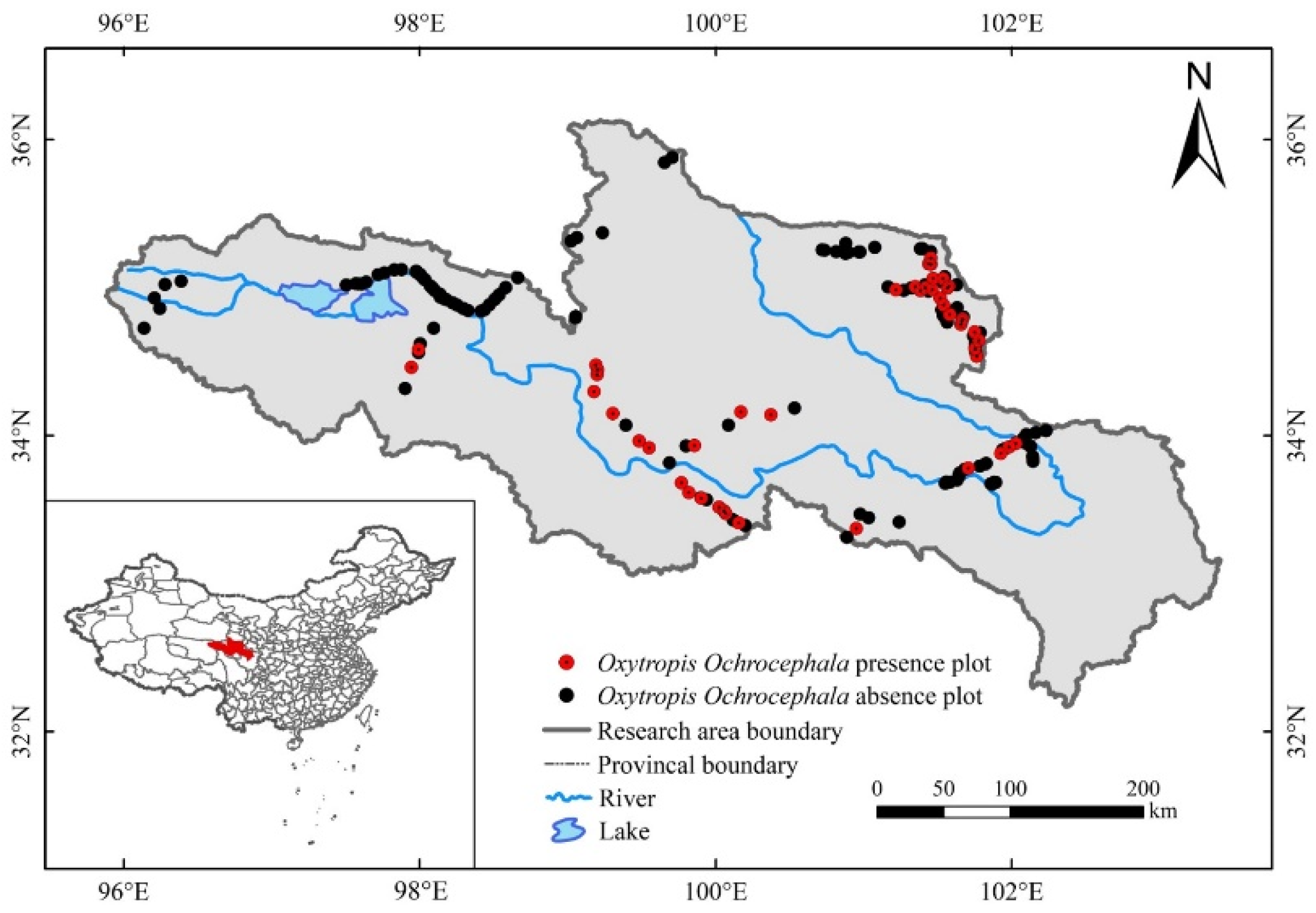
The SRYR (95°50′–103°30′E, 32°30′–36°10′N, mean altitude ~4000 m) lies in northeastern QTP (Figure 1); it is a critical ecological barrier on the QTP and one of the most important freshwater resources in China [29]. The SRYR covers an area of approximately 105,190 km2, characterized by low annual temperatures, large diurnal temperature differences, seasonal precipitation extremes, intense evaporation, and strong solar radiation [4]. It is a fragile eco-environment that is sensitive to climate change. The annual average precipitation decreases from the southeast to northwest, ranging from 200 to 700 mm, and annual temperature is between −4 °C and 2 °C [30]. The degraded grassland accounts for 36.5% of the available grassland in SRYR, of which 13.13% are poisonous weed-type degraded grassland [31]. Poisonous weeds account for 50–70% of poisonous weed type degraded grassland, which leads to a significant decline in grassland utilization [32]. The soils are mainly alpine steppe soils and alpine frozen soils [33]. The dominant plants are Sedge and Gramineae [34].
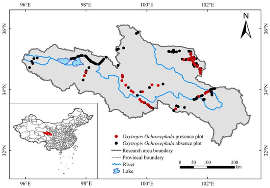
Figure 1.
Distribution of sampling sites (work points) and information about O. ochrocephala present–absence in the source region of Yellow River.
2.2. Field Aerial Photo Collection and Analysis
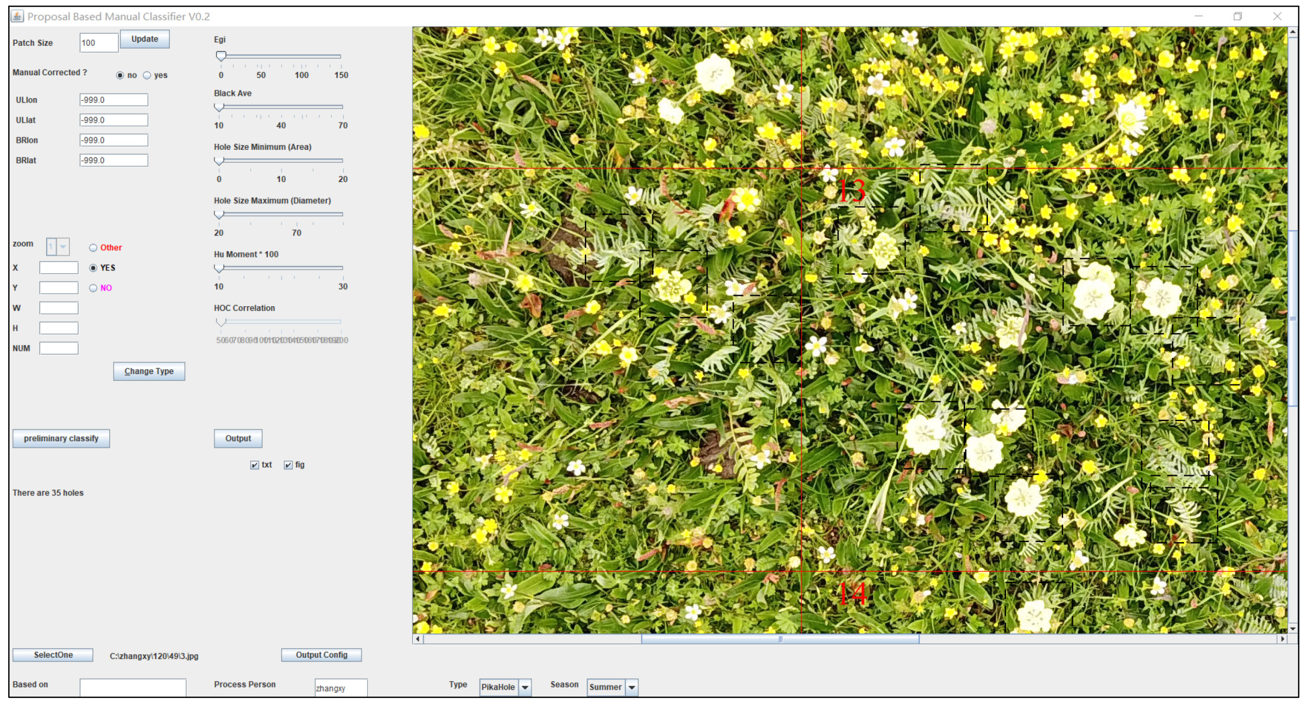
Field survey data of O. ochrocephala were collected by UAV during the peak growing season (July to September), from 2018 to 2020 (Figure 1). FragMAP system (installed and operated on Huawei M5, Shenzhen, China) was used to control the UAV, flying automatically along Belt routes (one inbuilt fly modes of FragMAP). Briefly, a commercial DJI MAVIC 2, equipped with a standard built-in 12-megapixel RGB camera (DJI Innovation Company, Shenzhen, China), was used to take aerial photographs vertically. At the sampling sites (the areas are representative and suitable for UAV flying), work points were used to mark the sampling positions on the map of FragMAP, which would be convenient for subsequent monitoring activities. Under each work point, we set one Belt route (the coverage area of each Belt route was 40 m × 40 m) with 16 fixed waypoints (monitoring points for the positions where the aerial photographs were taken) (Figure 2b). The height was set as 2 m from ground (2.6 m × 3.5 m on the ground) [35,36], and the ground sampling distance (GSD) was ~0.09 cm (Figure 2a). The pinnate compound leaves of O. ochrocephala are 5–19 cm in length; therefore, it is feasible to identify O. ochrocephala clearly on the aerial photographs (Figure 3). A total of 202 work points were set in SRYR, and 3232 aerial photographs were obtained. At each work point (202 in total), the presence–absence information was extracted visually by a software proposal classifier (Figure 3), which was independently developed by the Institute of Fragile Eco-Environment, Nantong University, based on Java [28]. Experimenters detect the objectives (O. ochrocephala in this study) visually and mark them by black rectangle on the interactive interface, on which any position could be located, based on the location of the aerial photograph and relative location (based on pixels) (Figure 3). In this study, once O. ochrocephala appeared in any photograph of the work point (the Belt route, contains 16 photographs), the work point would be recorded as a present sampling site; if no O. ochrocephala appeared in any aerial photograph, the work point would be recorded as an absence sampling site. The information could be exported by proposal classifier. A total of 48 presence records and 154 absence records in the SRYR were obtained for constructing the models (Figure 1).
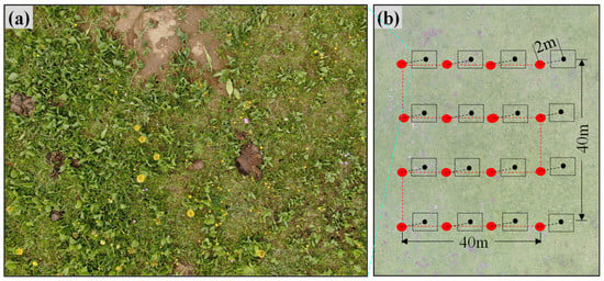
Figure 2.
Belt mode of FragMAP system. (a) UAV took aerial photographs at 2 m vertically, and (b) flying route of Belt mode.
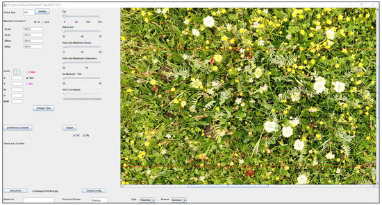
Figure 3.
Information extraction of O. ochrocephala, based on a proposal classifier software (developed by Yi [28]) on aerial photographs. The dash rectangles indicate the areas that O. ochrocephala present, the red lines and numbers are the marks generated automatically and used for making sure that all the areas had been checked.
2.3. Environmental Variables
In order to work out the geographic distribution of a suitable habitat of a target species, a set of characteristics about this species must be defined. In this study, 19 bioclimatic variables were used, which were obtained from the WorldClim database (www.worldclim.org/current (accessed on 13 December 2021)). The bioclimatic variables include annual mean temperature, mean diurnal range of temperature, isothermality, temperature seasonality, the max temperature of the warmest month, min temperature of the coldest month, temperature annual range, mean temperature of the wettest quarter, mean temperature of the driest quarter, mean temperature of the warmest quarter, mean temperature of the coldest quarter, annual precipitation, precipitation of the wettest month, precipitation of the driest month, precipitation seasonality, precipitation of the wettest quarter, precipitation of the driest quarter, precipitation of the warmest quarter, and precipitation of the coldest quarter. These variables were generated using averaged interpolated climate data, during the period from 1950 to 2010; the resolution was 30″ (1 km × 1 km) and marked the variables as climate 1 to 19 in turn (Table A1).
Besides, in order to improve the accuracy of the SDMs, 3 terrain variables and 8 soil variables were introduced. Terrain variables were introduced from the Shuttle Radar Topography Mission (SRTM) data (with a spatial resolution of 90 m × 90 m), derived from the US Geological Survey Administrative (www.usgs.gov (accessed on 13 December 2021)). QGIS Desktop was used to extract slope and aspect, according to the surface analysis of elevation data. A total of three terrain variables of elevation, aspect, and slope were resampled to the spatial resolution of 1 km × 1 km and marked as DEM 1 to 3 in turn (Table A1). Soil variables (spatial resolution of 1 km × 1 km) were obtained from SoilGrids (www.soilgrids.org (accessed on 13 December 2021)). Eight soil variables, i.e., soil thickness, soil organic carbon storage at 0.3–0.6 m depth, soil bulk density, soil clay content, soil coarse debris volume, soil silt content, soil sediment concentration, and soil pH at 0.3 m depth, were marked as soil 1 to 8 in turn (Table A1).
The same bioclimatic variables were projected into the future. Potential values for bioclimatic variables for future climate conditions in the 2050s and 2070s were derived from two representative concentration pathways (RCPs) of the medium greenhouse gas emission scenario (RCP4.5) and highest greenhouse gas emission scenario (RCP8.5), based on the BCC-CSM 1.1 (Beijing Climate Center Climate System Model Version 1.1) climate model [37,38].
2.4. Model Simulation
2.4.1. Environmental Variables Preprocessing
To reduce multicollinearity in the dataset for the environmental variables, the Pearson correlation coefficients between each pair of variables were calculated. When the correlation coefficients between two environmental variables are highly correlated (|r| > 0.8), one of them will be eliminated. The average importance values of environmental variables were calculated (n = 10, simulation times) and arranged in reverse order.
2.4.2. Model Construction and Evaluation
BIOMOD includes 10 SDMs: generalized linear model (GLM), generalized boosted regression model (GBM), generalized additive model (GAM), classification tree analysis (CTA), artificial neural networks (ANN), surface range envelope (SRE), flexible discriminant analysis (FDA), multivariate adaptive regression splines (MARS), random forest (RF), and maximum entropy model (MaxEnt) [39]. The applicability of different models can be evaluated by calculating the model accuracy with different indexes to screen out the best model.
To evaluate the quality of predictions, the input samples were randomly divided into two subsets, 70% of the total samples were used as training samples, whereas the other 30% were used for evaluation [40].
To validate the robustness of the evaluation for the SDMs, threshold-independent receiver operating characteristic (ROC) analysis was used. The area under the ROC curve (AUC) was examined for additional precision analysis, and the AUC could be obtained by calculating the area below the ROC curve. The value of AUC ranges between 0.5 and 1. A higher AUC indicates more accurate results [41].
2.4.3. Construction of Ensemble Model
The construction of the ensemble model, followed with the method of Guo et al. [22]. Briefly, the range of simulation results were firstly adjusted from [0, 1000] to [0, 1], and then the selected models (based on their accuracy scores) were integrated, through the weighted average method. The model weight is the ratio of the AUC value of a single model to the sum of the AUC values of the selected models. The calculation formula is as follows:
where Wj represents the weight of the jth model, rj represents the AUC value of the jth model, and h means the number of models in an ensemble model.
Finally, the normalized results of a single model were multiplied by the corresponding weights in turn and then summed to build an ensemble model and calculate the potentially suitable habitat distribution index of O. ochrocephala in the study area. The calculation formula is as follows:
where yi represents the comprehensive index [0, 1] of the potentially suitable habitat distribution of O. ochrocephala in the grid (i); wj represents the weight of the model (j) and xij is the value of the grid (i) in the model (j). A yi value closer to 1 means that the distribution probability is higher in the grid (i), i.e., it is more suitable for the growth of O. ochrocephala. In this study, habitat suitability was divided into four probability classes: 0–0.25, 0.26–0.50, 0.51–0.75, and 0.76–1.00, representing the unsuitable, low suitable, moderately suitable, and high suitable habitats, respectively. The distribution probability and area percentage of different suitable habitats of O. ochrocephala were calculated based on 10 simulation results.
2.4.4. Importance of Environmental Variables
To clarify the effects of environmental variables on the spatial distribution of O. ochrocephala, the importance of each environmental variable was calculated to the prediction results by using the factor importance calculation function of BIOMOD. Briefly, the dataset containing all environmental variables were defined as “reference dataset”, while the dataset from after eliminating one of the environmental variables randomly was defined as “test dataset”. The two datasets were used to predict and calculate the simple correlation of prediction results (Pearson correlation). The main affecting factors were ranked based on the average values of explaining variables in the suitable models.
2.4.5. Response of Habitat Suitability to Environmental Variables
The distribution of O. ochrocephala is affected by various environmental variables, so the relationship between its habitat suitability and a specific environmental variable is not always linear. Therefore, an appropriate parametric measure should be implemented when examining the response of habitat suitability of O. ochrocephala to environmental variables. The GAM could be applied to better describe the nonlinear relationships between explanatory variables and a response variable [42]. The package mgcv, in R language [43], was used to establish the GAM. The model can be expressed as:
where Y is the distribution probability of O. ochrocephala, fi(xi) represents the single single-variable function used to explain variable xi, and ε is the random variable.
3. Results
3.1. Model Accuracy Evaluation
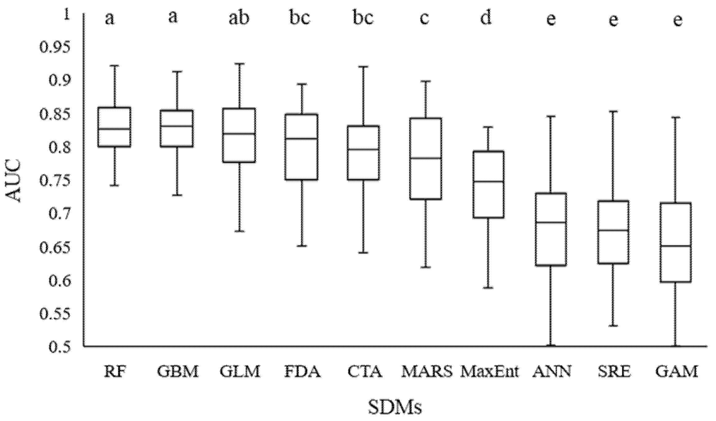
RF, GBM, and GLM performed best and were followed by FDA, CTA, MARS, MaxEnt, ANN, SRE, and GAM, respectively (p < 0.05) (Figure 4). Six models were selected, based on their accuracy scores: RF, GBM, GLM, FDA, CTA, and MARS (AUC value > 0.75, Figure 4). Based on the weighted average method, an ensemble model was built, according to the best results of the 6 SDMs, and the AUC maximum values were 0.921, 0.912, 0.924, 0.893, 0.919, and 0.897, respectively.

Figure 4.
Accuracy of the 10 species-distribution models of BIOMOD, based on AUC values (n = 10). The different letters on the bars indicate significant differences among the modes at the level of p < 0.05.
3.2. Screening and Importance of Environmental Factors
The annual mean temperature, mean diurnal range of temperature, isothermality, annual precipitation, precipitation of the driest period, elevation, aspect, slope, soil organic carbon storage, soil silt content, and soil pH were retained as environmental factors (Figure 5). Among the 12 environmental variables used to establish the model, the importance of annual precipitation (climate_12) and annual mean temperature (climate_1) exhibited the highest weight. Soil pH at 0.3 m depth (soil_8), elevation (DEM_1) had moderate importance, whereas the other variables, including soil organic carbon storage, isothermality, etc., showed low weight and, thus, indicated limited influence on the suitable habitat distribution of O. ochrocephala (Table 1).
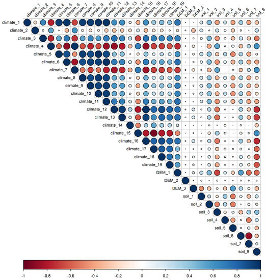
Figure 5.
The correlation among the environment variables. The size of the circles indicates the correlation between two environment variables.

Table 1.
Importance of the environment variables.
3.3. Relationship between Habitat Suitability and Environmental Variables
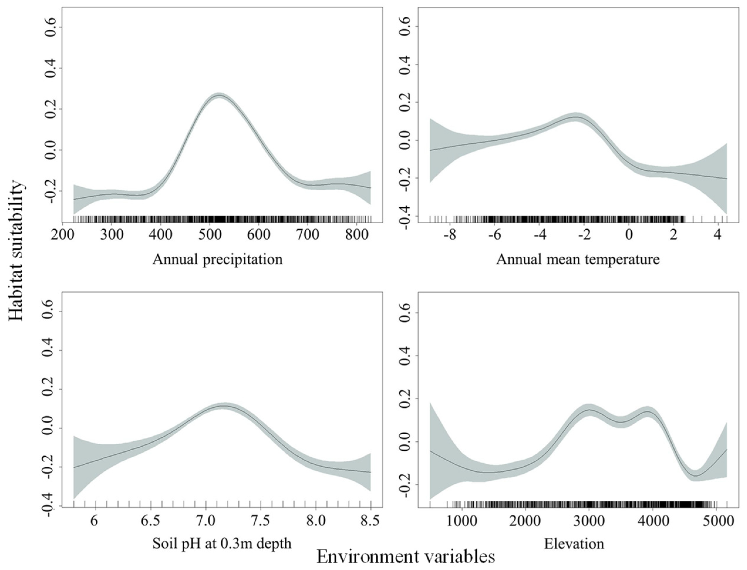
Based on the relationships between habitat suitability of O. ochrocephala and environmental variables (Figure 6), the highest suitability occurred when the annual precipitation (climate_12) ranged from about 440 mm to 615 mm, as well as an annual mean temperature (climate_1) from about −6 °C to −1 °C, soil pH at 0.3 m depth (soil_8) from about 6.8 to 7.5, and elevation (DEM_1) from about 2500 m to 4200 m.
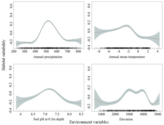
Figure 6.
Fitting curves of habitat suitability and main environmental variables, based on the generalized additive model (GAM).
3.4. The Potential Distribution of O. ochrocephala
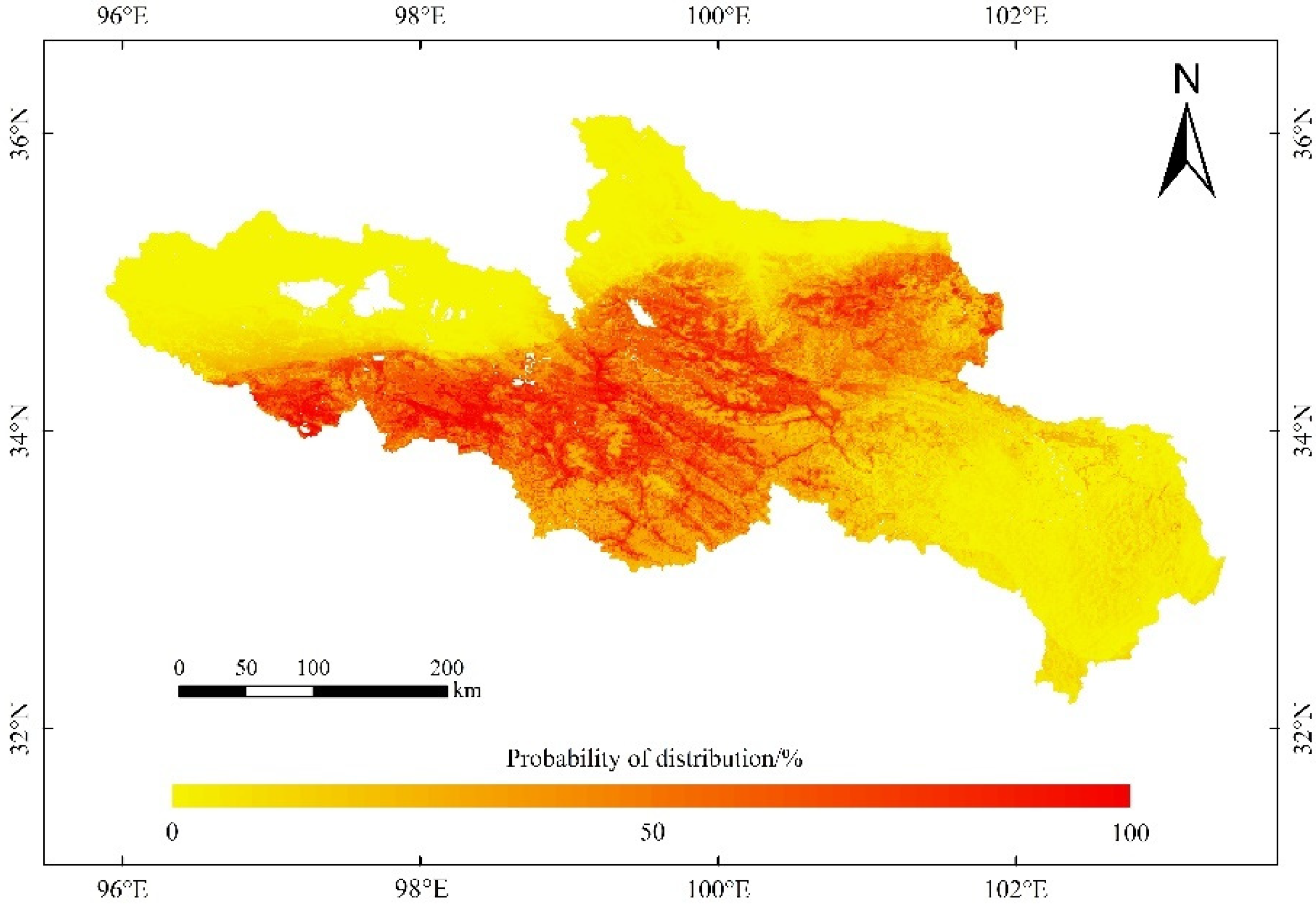
Overall, the potential distribution of the O. ochrocephala probability was 26.95% (Figure 7 and Figure 8). Furthermore, the distribution ranges, estimated by the six different SDMs, were similar. O. ochrocephala are mainly distributed in the southwest, middle, and northeast of the SRYR (Figure 7 and Figure 8).
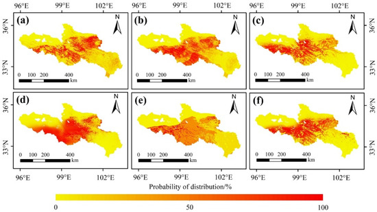
Figure 7.
Potential distribution of O. ochrocephala in the SRYR, based on single models: (a) RF, (b) GBM, (c) GLM, (d) FDA, (e) CTA, and (f) MARS.

Figure 8.
Potential distribution of O. ochrocephala in the source region of the Yellow River, under the current environmental scenario, based on the ensemble model, consisting of RF, GBM, GLM, FDA, CTA, and MARS.
Furthermore, according to the ensemble model, the suitable habitats of O. ochrocephala are mainly distributed in the southwest, middle, and northeast of the SRYR (Figure 8). In the SRYR, the high suitable habitat of O. ochrocephala only accounts for 2.65%, followed by moderately suitable habitat (16.98%), low suitable habitat (24.99%), and unsuitable habitat (55.38%) (Figure 8).
3.5. Prediction of O. ochrocephala Distribution under Climate Change Scenarios
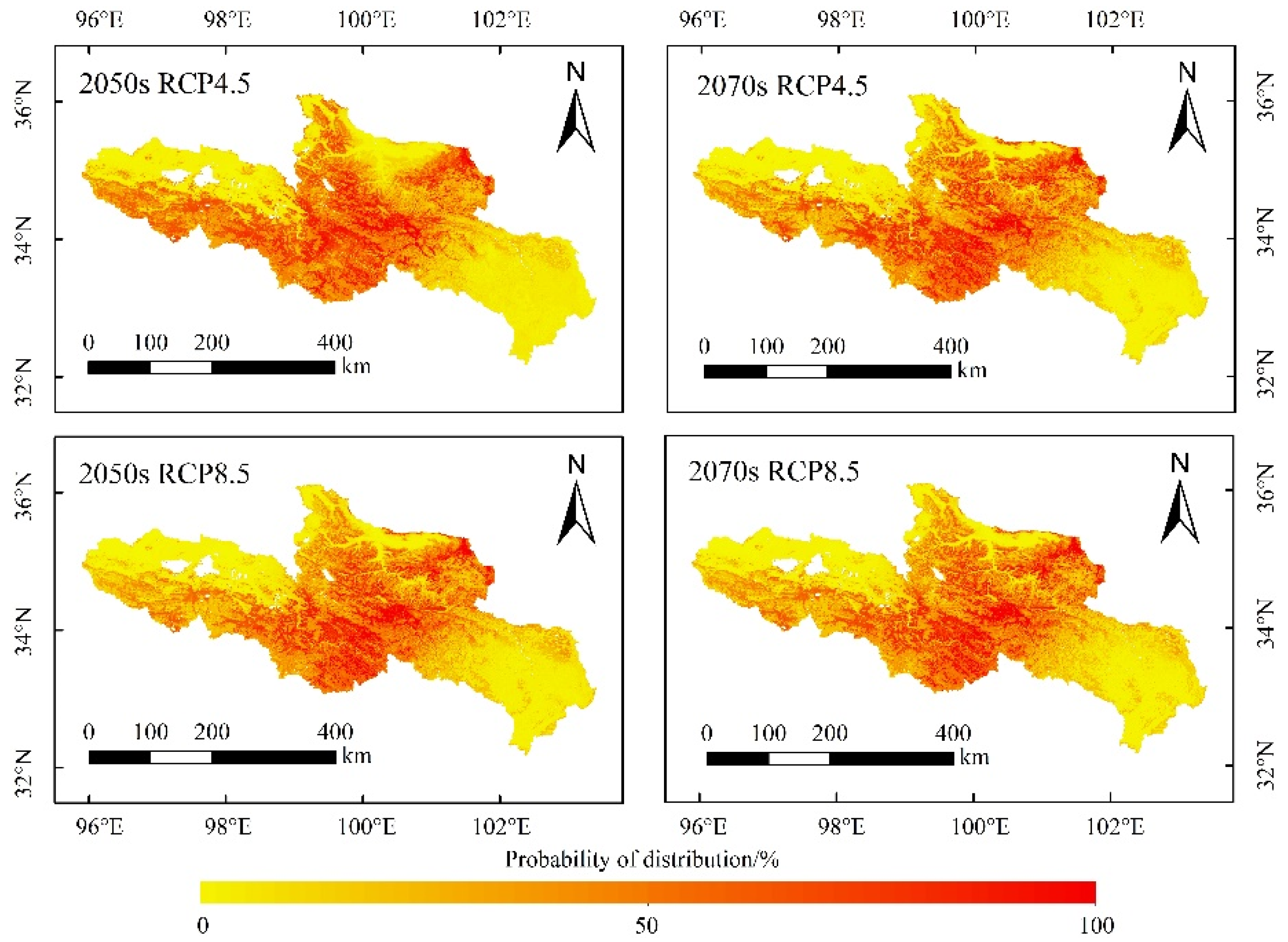
Annual precipitation and annual mean temperature were used to predict the future suitable distribution, for the reason that the two variables played a major role in the potential distribution of O. ochrocephala. Moreover, it is hard to simulate the future soil and DEM data. It was the same to the potential distribution prediction, six SDMs (RF, GBM, GLM, FDA, CTA, and MARS) were selected to establish the ensemble model and predicted the distribution of O. ochrocephala in the future (Figure 9).
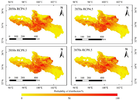
Figure 9.
Future distribution of O. ochrocephala in the source region of the Yellow River, under the future environmental scenario, based on the ensemble model, consisting of RF, GBM, GLM, FDA, CTA, and MARS.
The distribution probability of O. ochrocephala was not significantly different between the 2050s and 2070s, under the RCP4.5 or RCP8.5 scenario (Table 2). Meanwhile, it tended to increase under RCP8.5 scenario in the 2050s and 2070s (Table 2).

Table 2.
The distribution probability (±SE) of O. ochrocephala in the source region of the Yellow River, under the current period, 2050s and 2070s, based on RCP4.5 and RCP8.5 scenarios.
The area ratio of suitable habitats of O. ochrocephala did not significantly change, except, at the low suitable habitats (0.26–0.50), it could decrease in the future, both under the RCP4.5 and RCP8.5 scenarios (Table 3).

Table 3.
The area percentage (±SE) of different suitable habitats of O. ochrocephala in the source region of the Yellow River, under the current period, 2050s and 2070s, based on RCP4.5 and RCP8.5 scenarios.
4. Discussion
4.1. Potential Distribution of O. ochrocephala and Main Influence Variables
Recently, researchers and managers have paid more attention to the role that O. ochrocephala plays in the stability mechanism of the alpine grassland ecosystem and sustainable development of animal husbandry [44]. Previous studies illuminate that O. ochrocephala is widely distributed in the Qinghai Province, mainly distributed around Qinghai Lake, Huangnan, Guoluo, and Yushu Tibetan Autonomous Prefecture [45]. However, no research focuses on its spatiotemporal distribution pattern, based on scientific assessment at a reginal scale (e.g., in SRYR of this study). In this study, the areas that were clarified with high distribution probability were mainly in the southwest, middle, and northeast of SRYR (Figure 9), which is consistent with the previous research results.
Rainfall and temperature are of the most important factors shaping the function and structure of plants [46,47]. Similarly, in this study, annual precipitation (climate_12) and annual mean temperature (climate_1) were the two most important environmental variables in the establishment of the SDMs, and the accumulated effects exceeded 60% (Table 1). Based on the fitting curves of habitat suitability and environmental variables, the highest suitability of O. ochrocephala occurred when annual precipitation (climate_12) ranged from about 440 mm to 615 mm, annual mean temperature (climate_1) ranged from about −6 °C to −1 °C, soil pH ranged from about 6.8 to 7.5, and elevation ranged from about 2500 m to 4200 m. Our results agree with the conclusion of Huang [48], that is O. ochrocephala mainly grows in river beach grassland, arid desert grassland, and saline-alkali beach land at low altitude with low rainfall and strong light. This also agrees with the previous suggestion that O. ochrocephala is a plant adapted to the ecological environments with an altitude of about 2800 m, precipitation of 350 mm to 500 mm, and average annual temperature of −3 °C to −0 °C [49].
In this study, only environmental variables, such as climate, terrain, and soil, were focused. However, the intraspecific and interspecific relationships of the species and potential human disturbance were not determined. For instance, the migration ability of species, interaction between species, livestock grazing, and land-use change [50] may also influence the distribution of O. ochrocephala. It may be another potential reason for the low AUC values of SDMs. Future research could explore the appropriate datasets of microhabitat and human activities factors to improve the accuracy of prediction.
4.2. Changes in Distribution of O. ochrocephala in the Future
Several studies have tended to predict the species suitable habitat under climate change using the ensemble model [23,51,52]. Global warming promotes vegetation growth, and it has been revealed that temperature has a positive effect on alpine steppe, by accelerating the process of alpine phenology and prolonging the growing season on the QTP [53]. The RCP4.5 scenario indicates that the greenhouse gas emissions are moderately stable. It is assumed that the global annual greenhouse gas emissions (calculated as CO2) will peak around 2040 and then decrease. The RCP8.5 scenario indicates that the greenhouse gas emissions are large, and the ecological environment has little improvement. By 2100, the concentration of CO2 will be 3–4 times higher than that of before the industrial revolution, and some species with weak diffusion and migration capacity will face the risk of reducing (or even the extinction of) suitable habitats [54]. In this study, the distribution range of O. ochrocephala will not change significantly in the future, as they will still mainly distribute in the southwest, middle, and northeast of the SRYR, under the RCP4.5 and RCP8.5 scenarios (Figure 9). However, the distribution probability of O. ochrocephala in the SRYR will increase continuously, especially under RCP8.5 scenario (Table 2, p < 0.05 under RCP8.5 scenario). The results indicate that the continuous warming could result in the extension of O. ochrocephala. These results are different from that of the former studies, which focus on the spatiotemporal distribution of Stipa purpurea Griseb (fine forage) and reveals that a continuous rise in temperature could have a negative effect on vegetation [55,56]. Our results could play an important role in controlling and utilizing O. ochrocephala reasonably in the SRYR. For instance, removing O. ochrocephala effectively, based on the distribution pattern, could promote the production of livestock-liked silage [57]. Therefore, predicting the distribution of poisonous weed (e.g., O. ochrocephala) accurately, on a broad scale, is beneficial to both establishing reasonable management practices and animal husbandry in alpine grassland systems.
4.3. UAV Provides Basic Driving Data for a Niche Model
Complete and accurate data of species distribution is the premise of species distribution simulation [58]. However, traditional on-the-ground survey methods feature low efficiency, inconsistent standards, high labor cost, and a small observation range [59]. Moreover, due to the short growing season and fragile habitats of plants on QTP, it is difficult to complete large-scale investigation and sampling work in a limited time [17,52]. Virtual herbarium and literature search is another commonly used way to obtain basic drive data [60], while it is generally lacking timeliness and accurate geographic location information. Moreover, it is a kind of passively acquire data, and the datasets are often featured with insufficient and limited representativeness. An efficient, accurate, and suitable method for long-term and fixed-point monitoring is essential to accurately simulate and predict the spatiotemporal distribution of species. In this study, the UAV-based method is time and labor-saving, high-efficiency, low-cost, and non-destructive, overcoming the shortages of traditional methods. Therefore, it is suitable for large-scale investigations with few limitations. The data acquisition process, based on the FragMAP system, could be divided into two components, i.e., field sampling and indoor information extraction [38,61]. On the one hand, this method significantly improved the efficiency of field sampling (aerial photographs) and reduced the spatiotemporal constraints and operators’ activities. Meanwhile, it avoided unnecessary damage to the sampling area. On the other hand, FragMAP provides standardized, long-term, and fixed-point basic data for establishing SDMs. It not only ensures the accuracy and standard of basic drive data but also provides the foundation for model verification. Moreover, the species information collected indoors has several advantages, e.g., flexible time, standardization, and cooperation, which is beneficial to the efficiency and accuracy of species information.
In this study, visual species recognition was mainly used to extract the presence–absence information, and the efficiency is relatively low. Therefore, in a further study, a large number of obtained training samples (for example, O. ochrocephala selected manually can be automatically extracted and saved by proposal classifier, Figure 3) will play a key role in the subsequent automatic object identification [61,62]. Then, machine learning algorithms, such as convolution neural network and random forest, will identify target species automatically [63].
5. Conclusions
This study explored the feasibility of using UAV-based datasets for SDMs, identified the habitat distribution of O. ochrocephala and predicted its spatial distribution, under two scenarios of climate change. Meanwhile, the dominant variables that affect its spatiotemporal distribution of O. ochrocephala were explored. The results show that O. ochrocephala is mainly distributed in the southwest, middle, and northeast of the SRYR, and the distribution probability will increase under the scenario of RCP8.5. This study provides a reference for controlling and utilizing O. ochrocephala in the SRYR, which is beneficial for monitoring and predicting the spatiotemporal distribution of poisonous weeds on a large scale. It could also provide a necessary theoretical and practical basis for the sustainable development of the alpine grassland ecosystem and animal husbandry. Based on innovative UAV-based method, a large number of basic sampling data of O. ochrocephala could be used as the initial driving data. Nevertheless, the spatiotemporal distribution of the samples is usually heterogeneous. Hence, the distribution prediction of O. ochrocephala could potentially be affected to some extent. In future studies, it would be beneficial to improve the accuracy of plant spatiotemporal distribution prediction by improving the uniformity of field samples and making them evenly distributed in the study area.
Author Contributions
Conceptualization, S.Y. and Y.S.; methodology, X.Z. and Y.S.; software, Y.S., X.Z. and Y.Y.; validation, X.Z., Y.Y., Z.Z. and H.Y.; formal analysis, X.Z.; investigation, X.Z., Q.M., H.Y., M.L., Y.Y. and J.M.; resources, S.Y.; data curation, S.Y. and X.H.; writing—original draft preparation, X.Z. and Y.Y.; writing–review and editing, S.Y., X.H. and Y.S.; visualization, X.Z. and Z.Z.; supervision, S.Y.; project administration, Y.S.; funding acquisition, S.Y. All authors have read and agreed to the published version of the manuscript.
Funding
This research was funded by the National Natural Science Foundation (31901393, 42071056, 41801023), Natural Science Foundation of Jiangsu Province (BK20201439), National University’ Innovation and Entrepreneurship Training Program (202110304040Z), and Natural Science Foundation of Qinghai Province (2019-0301-ZJC-0265).
Institutional Review Board Statement
Not applicable.
Informed Consent Statement
Not applicable.
Data Availability Statement
19 bioclimatic variables were used, which were obtained from the WorldClim database (www.worldclim.org/current (accessed on 13 December 2021)); Terrain variables were introduced from the Shuttle Radar Topography Mission (SRTM) data (with a spatial resolution of 90 m × 90 m), derived from the US Geological Survey Administrative (www.usgs.gov (accessed on 13 December 2021)); Soil variables (spatial resolution of 1 km × 1 km) were obtained from SoilGrids (www.soilgrids.org (accessed on 13 December 2021)).
Acknowledgments
We are grateful to the Three-River-Source National Park Administration for helping us to collect the field data. We also thank four anonymous reviewers for their constructive comments, which have significantly improved the article.
Conflicts of Interest
The authors declare no conflict of interest.
Appendix A

Table A1.
Code of the environment variables.
Table A1.
Code of the environment variables.
| Code | Environmental Variables |
|---|---|
| climate_1 | Annual mean temperature |
| climate_2 | Mean diurnal range of temperature |
| climate_3 | Isothermality |
| climate_4 | Temperature seasonality |
| climate_5 | Max temperature of the warmest month |
| climate_6 | Min temperature of the coldest month |
| climate_7 | Temperature annual range |
| climate_8 | Mean temperature of the wettest quarter |
| climate_9 | Mean temperature of the driest quarter |
| climate_10 | Mean temperature of the warmest quarter |
| climate_11 | Mean temperature of the coldest quarter |
| climate_12 | Annual precipitation |
| climate_13 | Precipitation of the wettest month |
| climate_14 | Precipitation of the driest month |
| climate_15 | Precipitation seasonality |
| climate_16 | Precipitation of the wettest quarter |
| climate_17 | Precipitation of the driest quarter |
| climate_18 | Precipitation of the warmest quarter |
| climate_19 | Precipitation of the coldest quarter |
| DEM_1 | Elevation |
| DEM_2 | Aspect |
| DEM_3 | Slope |
| soil_1 | Soil thickness |
| soil_2 | Soil organic carbon storage at 0.3–0.6 m depth |
| soil_3 | Soil bulk density at 0.3 m depth |
| soil_4 | Soil clay content at 0.3 m depth |
| soil_5 | Soil coarse debris volume at 0.3 m depth |
| soil_6 | Soil silt content at 0.3 m depth |
| soil_7 | Soil sediment concentration at 0.3 m depth |
| soil_8 | Soil pH at 0.3 m depth |
References
- Hughes, L. Biological consequences of global warming: Is the signal already apparent? Trends Ecol. Evol. 2000, 15, 56–61. [Google Scholar] [CrossRef]
- Bertrand, R.; Lenoir, J.; Piedallu, C.; Riofrío-Dillon, G.; de Ruffray, P.; Vidal, C.; Pierrat, J.C.; Gégout, J.C. Changes in plant community composition lag behind climate warming in lowland forests. Nature 2011, 479, 517–520. [Google Scholar] [CrossRef]
- Ding, Y.J.; Yang, J.P.; Liu, S.Y.; Chen, R.S.; Wang, G.X.; Shen, Y.P.; Wang, J.; Xie, C.W.; Zhang, S.Q. Exploration of eco-environment range in the source regions of the Yangtze and Yellow Rivers. Acta Geogr. Sin. 2003, 58, 519–526. [Google Scholar]
- Ge, J.; Meng, B.; Liang, T.; Feng, Q.; Gao, J.; Yang, S.; Huang, X.; Xie, H. Modeling alpine grassland cover based on MODIS data and support vector machine regression in the headwater region of the Huanghe River, China. Remote Sens. Environ. 2018, 218, 162–173. [Google Scholar] [CrossRef]
- Ren, J.Z.; Lin, H.L. Assumed plan on grassland ecological reconstruction in the source region of Yangtse River, Yellow River and Lantsang River. Acta Pratac. Sin. 2005, 14, 1–8. [Google Scholar]
- Chen, Q.G. Grassland deterioration in the source region of the Yangtze-Yellow rivers and integrated control of the ecological environment. Acta Pratac. Sin. 2007, 16, 10–15. [Google Scholar]
- Wang, P.; Lassoie, J.P.; Morreale, S.J.; Dong, S.K. A critical review of socioeconomic and natural factors in ecological degradation on the Qinghai-Tibetan Plateau, China. Rangel. J. 2015, 37, 1–9. [Google Scholar] [CrossRef]
- Liu, S.B.; Zamanian, K.; Schleuss, P.M.; Zarebanadkouki, M.; Kuzyakov, Y. Degradation of Tibetan grasslands: Consequences for carbon and nutrient cycles. Agric. Ecosyst. Environ. 2018, 252, 93–104. [Google Scholar] [CrossRef]
- Sun, R.Q.; Cheng, D.L.; Jia, Z.J.; Zhu, Z.Q. Studies on the chemical components of Oxtropis ochrocephala Bunge II. The structures of two triterpenoid taponins. Acta Chim. Sin. 1987, 45, 145–149. [Google Scholar]
- Lu, H.; Wang, S.S.; Zhou, Q.W.; Zhao, Y.N.; Zhao, B.Y. Damage and control of major poisonous plants in the western grasslands of China—A review. Rangel. J. 2012, 34, 329–339. [Google Scholar] [CrossRef]
- He, W.; Guo, L.W.; Fan, P.H.; Guo, B.; Fu, Y.P.; Wei, Y.H. Allelopathy and the rhizospere bacterial community structure of Oxytropis ochrocephala. Acta Prataculturae Sin. 2015, 24, 21–29. [Google Scholar]
- Deng, J.M.; Yang, S.Y.; Shen, H.M. Allelopathy of twelve poisonous plants. Acta Bot. Boreali-Occident. Sin. 2009, 29, 989–995. [Google Scholar]
- Bryan, J.A.; Berlyn, G.P.; Gordon, J.C. Toward a new concept of the evolution of symbiotic nitrogen fixation in the Leguminosae. Plant Soil 1996, 186, 151–159. [Google Scholar] [CrossRef]
- Pearce, J.; Ferrier, S. An evaluation of alternative algorithms for fitting species distribution models using logistic regression. Ecol. Model. 2000, 128, 127–147. [Google Scholar] [CrossRef]
- Stockwell, D.R.B.; Peterson, A.T. Effects of sample size on accuracy of species distribution models. Ecol. Model. 2002, 148, 1–13. [Google Scholar] [CrossRef]
- Guisan, A.; Thuiller, W. Predicting species distribution: Offering more than simple habitat models. Ecol. Lett. 2005, 8, 993–1009. [Google Scholar] [CrossRef]
- Raes, N.; Aguirre-Gutiérrez, J. A modeling framework to estimate and project species distributions in space and time. In Mountains, Climate and Biodiversity; Hoorn, C., Perrigo, A., Antonelli, A., Eds.; John Wiley & Sons: Chichester, UK, 2018. [Google Scholar]
- Martínez-Minaya, J.; Cameletti, M.; Conesa, D.; Pennino, M.G. Species distribution modeling: A statistical review with focus in spatio-temporal issues. Stoch. Environ. Res. Risk Assess. 2018, 32, 3227–3244. [Google Scholar] [CrossRef]
- Tessarolo, G.; Lobo, J.M.; Rangel, T.F.; Hortal, J. High uncertainty in the effects of data characteristics on the performance of species distribution models. Ecol. Indic. 2021, 121, 107147. [Google Scholar] [CrossRef]
- Thuiller, W.; Richardson, D.M.; Rouget, M.; Procheş, Ş.; Wilson, J.R.U. Interactions between environment, species traits, and human uses describe patterns of plant invasions. Ecology 2006, 87, 1755–1769. [Google Scholar] [CrossRef]
- Tanaka, K.R.; Torre, M.P.; Saba, V.S.; Stock, C.A.; Chen, Y. An ensemble high resolution projection of changes in the future habitat of American lobster and sea scallop in the Northeast US continental shelf. Divers. Distrib. 2020, 26, 987–1001. [Google Scholar] [CrossRef]
- Guo, Y.L.; Li, X.; Zhao, Z.F.; Zain, N. Predicting the impacts of climate change, soils and vegetation types on the geographic distribution of Polyporus umbellatus in China. Sci. Total Environ. 2019, 648, 1–11. [Google Scholar] [CrossRef] [PubMed]
- Araújo, M.B.; Peterson, A.T. Uses and misuses of bioclimatic envelope modeling. Ecology 2012, 93, 1527–1539. [Google Scholar] [CrossRef] [Green Version]
- Rominger, K.; Meyer, S. Application of UAV-based methodology for census of an endangered plant species in a fragile habitat. Remote Sens. 2019, 11, 719. [Google Scholar] [CrossRef] [Green Version]
- Guisan, A.; Thuiller, W.; Zimmermann, N.E. Habitat Suitability and Distribution Models: With Applications in R; Cambridge University Press: Cambridge, UK, 2017. [Google Scholar]
- Xiang, H.T.; Tian, L. Development of a low-cost agricultural remote sensing system based on an autonomous unmanned aerial vehicle (UAV). Biosyst. Eng. 2011, 108, 174–190. [Google Scholar] [CrossRef]
- Feng, Q.L.; Liu, J.T.; Gong, J.H. UAV remote sensing for urban vegetation mapping using random forest and texture analysis. Remote Sens. 2015, 7, 1074–1094. [Google Scholar] [CrossRef] [Green Version]
- Yi, S.H. FragMAP: A tool for long-term and cooperative monitoring and analysis of small-scale habitat fragmentation using an unmanned aerial vehicle. Int. J. Remote Sens. 2017, 38, 2686–2697. [Google Scholar] [CrossRef]
- Chu, H.B.; Wei, J.H.; Li, T.J.; Jia, K. Application of support vector regression for mid- and long-term runoff forecasting in “Yellow River Headwater” region. Procedia Eng. 2016, 154, 1251–1257. [Google Scholar] [CrossRef] [Green Version]
- Li, Q.; Yang, M.X.; Wan, G.N.; Wang, X.J. Spatial and temporal precipitation variability in the source region of the Yellow River. Environ. Earth Sci. 2016, 75, 594. [Google Scholar] [CrossRef]
- Wu, Q.; Zhou, Y.L. Analysis of ecological environment change and water resources vulnerability in the source region of the Yellow River. Water Resour. Protec. 2002, 4, 21–24. [Google Scholar]
- Yang, M.; Li, X.W.; Ma, J.X. Functioning of poisonous and harmful grasses on grassland and dilemma in ecosystem restoration and economic development. Chin. J. Ecol. 2005, 24, 1177–1181. [Google Scholar]
- Duan, H.C.; Xue, X.; Wang, T.; Kang, W.P.; Liao, J.; Liu, S.L. Spatial and temporal differences in alpine meadow, alpine steppe and all vegetation of the Qinghai-Tibetan Plateau and their responses to climate change. Remote Sens. 2021, 13, 669. [Google Scholar] [CrossRef]
- Yu, G.A.; Brierley, G.; Huang, H.Q.; Wang, Z.; Blue, B.; Ma, Y. An environmental gradient of vegetative controls upon channel planform in the source region of the Yangtze and Yellow Rivers. Catena 2014, 119, 143–153. [Google Scholar] [CrossRef]
- Sun, Y.; Yi, S.H.; Hou, F.J. Unmanned aerial vehicle methods makes species composition monitoring easier in grasslands. Ecol. Indic. 2018, 95, 825–830. [Google Scholar] [CrossRef]
- Qin, Y.; Sun, Y.; Zhang, W.; Qin, Y.; Chen, J.; Wang, Z.; Zhou, Z. Species monitoring using unmanned aerial vehicle to reveal the ecological role of Plateau Pika in maintaining vegetation diversity on the northeastern Qinghai-Tibetan Plateau. Remote Sens. 2020, 12, 2480. [Google Scholar] [CrossRef]
- Wu, T.W.; Song, L.C.; Li, W.P.; Wang, Z.Z.; Zhang, H.; Xin, X.G.; Zhang, Y.W.; Zhang, L.; Li, J.L.; Wu, F.H.; et al. An overview of BCC climate system model development and application for climate change studies. J. Meteorol. Res.-PRC 2014, 28, 34–56. [Google Scholar] [CrossRef]
- Huang, B.; YI, S.H.; Zhang, X.Y.; Ma, Q.S.; Xiang, B.; Du, J.X.; Ma, J.H.; Sun, Y. Distribution of Ligularia virgaurea in the source region of the Yellow River based on BIOMOD. Pratac. Sci. 2020, 37, 2198–2210. [Google Scholar]
- Huiller, W.T. BIOMOD—Optimizing predictions of species distributions and projecting potential future shifts under global change. Glob. Chang. Biol. 2003, 9, 1353–1362. [Google Scholar] [CrossRef]
- Fielding, A.; Bell, J. A review of methods for the assessment of prediction errors in conservation presence/absence models. Environ. Conserv. 1997, 24, 38–49. [Google Scholar] [CrossRef]
- Fawcett, T. An introduction to ROC analysis. Pattern Recognit. Lett. 2006, 27, 861–874. [Google Scholar] [CrossRef]
- De Bock, K.W.; Coussement, K.; Van den Poel, D. Ensemble classification based on generalized additive models. Comput. Stat. Data Anal. 2010, 54, 1535–1546. [Google Scholar] [CrossRef]
- R Core Team. R: A language and Environment for Statistical Computing; R Foundation for Statistical Computing: Vienna, Austria, 2020. [Google Scholar]
- Wang, W.T.; Gao, S.Y.; Wang, S.F. Predictive studies of potential invasive areas for four poisonous weeds in Gansu Grassland. Acta Ecol. Sin. 2019, 39, 5301–5307. [Google Scholar]
- Ji, Y.J.; Wang, L.Y. Study on poisonous plants of Oxytropis in Qinghai grassland. Sichuan Grassl. 2004, 106, 10–12. [Google Scholar]
- Yang, Y.; Li, X.; Kong, X.; Ma, L.; Hu, X.; Yang, Y. Transcriptome analysis reveals diversified adaptation of Stipa purpurea along a drought gradient on the Tibetan Plateau. Funct. Integr. Genom. 2015, 15, 295–307. [Google Scholar] [CrossRef]
- Wang, T.; Dan, Y.U.; Jiang-Feng, L.I.; Ke-Ping, M.A. Advances in research on the relationship between climatic change and tree-ring width. Chin. J. Plant Ecol. 2003, 27, 23–33. [Google Scholar]
- Huang, L.M. Investigation and control of poisonous weeds in natural grassland in Huangnan Prefecture. Sichuan Grassl. 2006, 5, 24–26. [Google Scholar]
- Shao, S.H.; Zheng, B.S.; Zhao, C.Z.; Yin, C.Q.; Lang, Y.B.; Zhang, A.L. Toxic grasses of Succuir recorded in The Travels of Marco Polo and their eco-environmental background. Pratac. Sci. 2004, 6, 62–66. [Google Scholar]
- Liu, X.T.; Yuan, Q.; Ni, J. Research advances in modelling plant species distribution in China. Chin. J. Plant Ecol. 2019, 43, 273–283. [Google Scholar] [CrossRef]
- Tabor, J.A.; Koch, J.B. Ensemble models predict invasive bee habitat suitability will expand under future climate scenarios in Hawai’i. Insects 2021, 12, 443. [Google Scholar] [CrossRef]
- Fang, Y.Q.; Zhang, X.H.; Wei, H.Y.; Wang, D.J.; Chen, R.D.; Wang, L.K.; Gu, W. Predicting the invasive trend of exotic plants in China based on the ensemble model under climate change: A case for three invasive plants of Asteraceae. Sci. Total Environ. 2021, 756, 143841. [Google Scholar] [CrossRef] [PubMed]
- Xu, M.H.; Peng, F.; You, Q.G.; Guo, J.; Tian, X.F.; Xue, X.; Liu, M. Year-round warming and autumnal clipping lead to downward transport of root biomass, carbon and total nitrogen in soil of an alpine meadow. Environ. Exp. Bot. 2015, 109, 54–62. [Google Scholar] [CrossRef]
- Urban, M.C. Accelerating extinction risk from climate change. Science 2015, 348, 571–573. [Google Scholar] [CrossRef] [Green Version]
- Xu, M.H.; Xue, X. Analysis on the effects of climate warming on growth and phenology of alpine plants. J. Arid Resour. Environ. 2013, 27, 137–141. [Google Scholar]
- Xu, M.H.; Xue, X. A research on summer vegetation characteristics & short-time responses to experimental warming of alpine meadow in the Qinghai-Tibetan Plateau. Acta Ecol. Sin. 2013, 33, 2071–2083. [Google Scholar]
- Chen, J.; Huang, W.Y.; Zhao, B.Y.; Mo, C.H. Effect of fermentation time on the quality and swainsonine content of Oxytropis ochrocephala silage. Prog. Vet. Med. 2019, 40, 77–81. [Google Scholar]
- Guo, Y.L.; Li, X.; Zhao, Z.F.; Wei, H.Y. Modeling the distribution of Populus euphratica in the Heihe River Basin, an inland river basin in an arid region of China. Sci. China 2019, 49, 537–553. [Google Scholar] [CrossRef]
- Sun, Y.; Hou, F.J.; Angerer, J.P.; Yi, S.H. Effects of topography and land-use patterns on the spatial heterogeneity of terracette landscapes in the Loess Plateau, China. Ecol. Indic. 2020, 109, 105839. [Google Scholar] [CrossRef]
- Huang, X.; Ma, L.; Chen, C.; Zhou, H.; Yao, B.; Ma, Z. Predicting the suitable geographical distribution of Sinadoxa corydalifolia under different climate change scenarios in the Three-River Region using the MaxEnt model. Plants 2020, 9, 1015. [Google Scholar] [CrossRef] [PubMed]
- Gao, Y.Y.; Ma, Q.S.; Zhang, X.Y.; Ma, J.H.; Yi, S.H.; Li, B.C.; Zhang, J.G.; Lu, X.M.; Sun, Y. Preliminary exploration of monitoring Gynaephora alpherakii using unmanned aerial vehicles (UAV). Pratac. Sci. 2020, 37, 2106–2114. [Google Scholar]
- Yang, Y.H.S.; Xi, X.Q.; Zhong, X.T.; Eisenhauer, N.; Sun, S.C. N addition suppresses the performance of grassland caterpillars (Gynaephora alpherakjj) by decreasing ground temperature. Ecosphere 2017, 8, e01755. [Google Scholar] [CrossRef] [Green Version]
- Jakovljevic, G.; Govedarica, M.; Alvareztaboada, F. A deep learning model for automatic plastic mapping using unmanned aerial vehicle (UAV) data. Remote Sens. 2020, 12, 1515. [Google Scholar] [CrossRef]
Publisher’s Note: MDPI stays neutral with regard to jurisdictional claims in published maps and institutional affiliations. |
© 2021 by the authors. Licensee MDPI, Basel, Switzerland. This article is an open access article distributed under the terms and conditions of the Creative Commons Attribution (CC BY) license (https://creativecommons.org/licenses/by/4.0/).

