Article

Random Forest Classification of Inundation Following Hurricane Florence (2018) via L-Band Synthetic Aperture Radar and Ancillary Datasets

by
Alexander M. Melancon
1,*,
Andrew L. Molthan
2,
Robert E. Griffin
1,
John R. Mecikalski
1,
Lori A. Schultz
2 and
Jordan R. Bell
2
1
Department of Atmospheric and Earth Science, University of Alabama in Huntsville, 320 Sparkman Dr. NW, Huntsville, AL 35805, USA
2
NASA Marshall Space Flight Center, Earth Science Branch, Huntsville, AL 35808, USA
*
Author to whom correspondence should be addressed.
Remote Sens. 2021, 13(24), 5098; https://doi.org/10.3390/rs13245098
Submission received: 20 October 2021 / Revised: 30 November 2021 / Accepted: 9 December 2021 / Published: 15 December 2021

Abstract

:
In response to Hurricane Florence of 2018, NASA JPL collected quad-pol L-band SAR data with the Uninhabited Aerial Vehicle Synthetic Aperture Radar (UAVSAR) instrument, observing record-setting river stages across North and South Carolina. Fully-polarized SAR images allow for mapping of inundation extent at a high spatial resolution with a unique advantage over optical imaging, stemming from the sensor’s ability to penetrate cloud cover and dense vegetation. This study used random forest classification to generate maps of inundation from L-band UAVSAR imagery processed using the Freeman–Durden decomposition method. An average overall classification accuracy of 87% is achieved with this methodology, with areas of both under- and overprediction for the focus classes of open water and inundated forest. Fuzzy logic operations using hydrologic variables are used to reduce the number of small noise-like features and false detections in areas unlikely to retain water. Following postclassification refinement, estimated flood extents were combined to an event maximum for societal impact assessments. Results from the Hurricane Florence case study are discussed in addition to the limitations of available validation data for accuracy assessments.

Graphical Abstract

1. Introduction

Flooding is a common occurrence across the United States and the world. In coastal areas, tropical cyclones can cause or exacerbate existing flooding issues through storm surge or excessive rainfall. NOAA’s National Center for Environmental Information (NCEI) reports that tropical cyclones and inland flooding were the second and third most frequent out of 290 billion-dollar disasters in the United States from 1980 to 2020. Tropical cyclones have caused the most damage (USD 1034 billion), have the highest average event cost (USD 19.9 billion), and are responsible for the highest number of deaths out of all disaster types (6593) [1]. Creating flood maps is an essential part of understanding the magnitude of a particular event and estimating impacts of a future occurrence. A broad audience, including government agencies and contractors, insurance agents, land developers, and community planners, views flood maps an estimated 30 million times each year for land management as well as mitigation, risk assessment, and disaster response purposes [2]. The accuracy of flood maps is crucial for these applications, where mistakes can be costly to the government, private businesses, and individuals in affected areas. Maps of water extent can be produced using a combination of visible and near-infrared imagery. These passive types of remote sensing depend on the reflection of solar radiation from the Earth’s surface and are therefore limited to daytime availability. The low reflectance of water in these bands makes it possible to map the extent of open-water bodies, but not water under vegetation [3]. Additional issues arise from clouds and their shadows which block the view of the surface, and immediate response to hurricane impacts using visible and near-infrared data is made difficult due to the extensive amount of coincident cloud cover blocking the view of floodwaters on the ground. The active transmission of energy from SAR instruments allows for image detection through clouds and data collection during day and night [4,5]. L-band SAR has an advantage over other bands in inundation detection due to its relatively longer (15–30 cm) wavelength, capable of penetrating further into the forest canopy and providing a view of flooding beneath [6,7,8]. An analysis of multifrequency SAR data performed by Ramsey et al. (2013) found that mapped wetland inundation via L-band ALOS PALSAR data offered higher correspondence to local inundation patterns than C-band ENVISAT ASAR imagery [9]. Currently, there are no active satellite missions that provide regular, openly available L-band SAR observations. NASA’s Jet Propulsion Laboratory (JPL) gathers L-band SAR data via their Uninhabited Aerial Vehicle Synthetic Aperture Radar (UAVSAR) instrument during field campaigns and specific event responses. The Gulfstream-III jet-mounted UAVSAR serves as a platform for data collection similar to the upcoming NASA–Indian Space Research Organization (ISRO) SAR mission known as NISAR, which will provide open access to L- and S-band imagery. Knowledge gained from UAVSAR data helps to inform the use of comparable L-band data from NISAR and other future SAR satellites. Before SAR data can be used for decision support, a deterministic approach is needed to identify inundated pixels. Supervised image classification schemes such as support vector machine (SVM) and classification and regression trees (CARTs) are widely used in remote sensing because of their ability to learn the characteristics of target classes from training samples and apply them to unclassified data [10]. The random forest (RF) classifier relies on an ensemble of CARTs to predict and vote on the most likely class [11]. It is computationally efficient and offers faster processing times than other machine learning techniques [12,13]. A comparison of land cover classification results from SVM and RF on polarimetric images from RADARSAT-2 (C-band) and AIRSAR (L-band) by Uhlmann and Kiranyaz (2014) concluded that RF provided the most stable results and highest accuracy throughout all classified images [14].
Given the advantages of L-band SAR in inundation detection and the proven skill of RF in SAR-based inundation mapping, an RF-based classification of UAVSAR data could potentially be useful in emergency response efforts. This study uses UAVSAR data processed using the Freeman–Durden polarimetric decomposition method in combination with ancillary datasets to determine how accurately areas of inundation can be identified using RF classification. An accuracy assessment is performed, following good practice methods for land cover classification outlined in Olofsson et al. (2014) [15]. Following postclassification cleanup, all available water extent determinations are combined to represent an event maximum. This event extent is then combined with datasets describing the distribution of the human population (LandScan 2018; [16]), buildings inferred from Microsoft Building Footprints [17], and roads (USGS National Transportation Dataset; [18]) throughout the domain of study to evaluate impacts in flooded areas.

2. Study Area and Materials

2.1. Study Area and Event Background

This project is focused on southeastern North Carolina shortly after Hurricane Florence impacted the region in September of 2018. Florence was the sixth named storm and the first major hurricane of the 2018 hurricane season, reaching a peak strength of ∼67 m s 1 (150 mph) on 11 September, a strong Category 4, according to the Saffir–Simpson scale, as it crossed the Atlantic. The storm made landfall near Wrightsville Beach, North Carolina, on 14 September as a ∼40 m s 1 (90 mph) Category 1 hurricane [19]. Once over land, the forward motion of the storm slowed to 0.89–1.34 m s 1 (2–3 mph), allowing for the accumulation of up to 91.44 cm (36 in.) of rain over four days for areas in southeastern North Carolina. United States Geological Survey (USGS) streamflow data indicate that 45 gauges in North Carolina recorded peaks within their top five streamflows, while 18 gauges set new streamflow records [20]. This massive influx of water extensively inundated the region. Nearly 97 km (60 mi) of Interstate 95, a major north–south thoroughfare, was closed due to flooding by 19 September and remained impassable through 23 September, over a week after the landfall of Florence [21]. In response to the extreme rainfall and subsequent flooding, NASA flew UAVSAR along several major river basins in the Carolinas to collect imagery for L-band SAR-based impact estimation and analysis. This study focused on four flight tracks along the Lumber and Cape Fear River basins in southeastern North Carolina. Data within the incidence angle range of 30–50° is available for a total area of approximately 208,500 km 2 (80,500 mi 2 ), portions of eleven counties. This region of North Carolina’s inner coastal plain is predominantly flat and gently declines in elevation toward the Atlantic Ocean, ranging from over 150 m in the eastern Appalachian foothills to near or below mean sea level along the coast. Inspection of National Land Cover Database (NLCD) 2016 data (Figure 1) indicates that the three most common land cover types are woody wetlands, evergreen forests, and cultivated croplands, representing over 77% of the combined study area [22]. The prevalence of vegetative cover in the study area suggests that much of the flooding would be obscured in visible imagery, limiting its utility for flood mapping activities.

2.2. Datasets and Preprocessing

2.2.1. UAVSAR Data

UAVSAR is a quad-pol L-band radar that operates at a frequency of 1.26 GHz and has a look angle range of 25° to 60° [23]. The system is intended for use on an uninhabited aerial vehicle (UAV) for repeating acquisitions over defined paths of interest. The radar instrument is currently operated from a NASA Gulfstream-III jet equipped with an onboard flight system that uses real-time GPS navigation to keep the flight path within 10 m of the desired track [24]. UAVSAR data were collected, processed, and made available via NASA JPL. The Alaska Satellite Facility Distributed Active Archive Center (ASF DAAC) provides open access to data collected by UAVSAR in addition to several other SAR sensors.
Fully polarimetric data from twelve flight lines across North and South Carolina were gathered from 17 to 23 September 2018, with up to six revisits, to support response efforts to Hurricane Florence. This data is radiometrically calibrated by NASA JPL and is available for download from the UAVSAR data portal at [25]. Four flight lines centered over the Lumber and Cape Fear Rivers were chosen for analysis due to their proximity and frequency of observations. Geographically projected multilook cross products and incidence angle files were obtained for each day available for these flight lines, referred to as LT1, LT2, CF1, and CF2, for a total of fifteen data swaths. Multilook is an SAR data-processing method that reduces speckle noise, eliminating the need for image filtering before classification [26].

2.2.2. UAVSAR Preprocessing

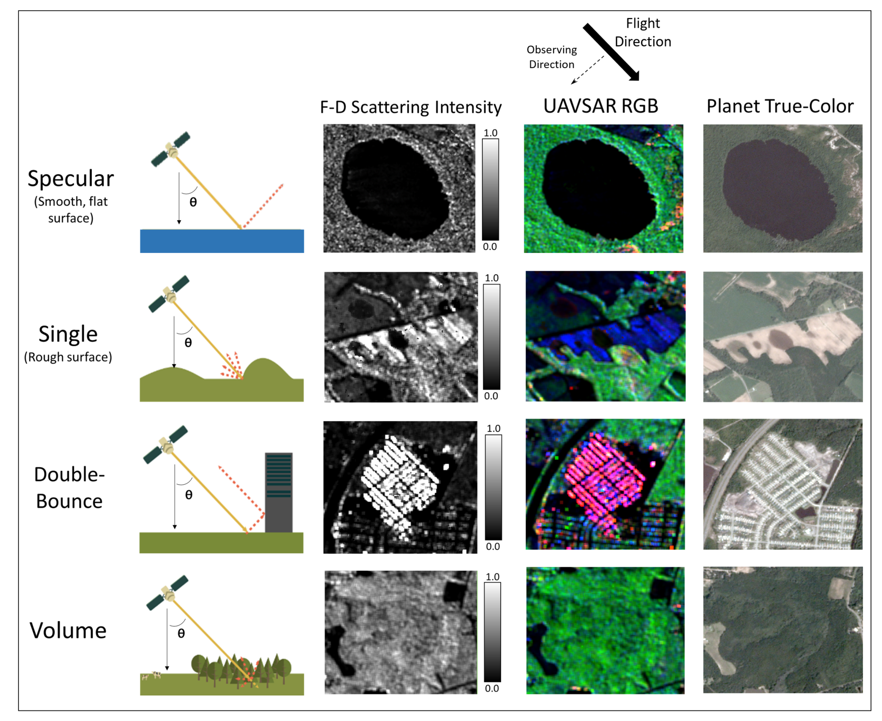
Fully polarimetric, or quad-pol, SAR sensors such as UAVSAR can transmit and receive signals from four horizontal and vertical orientations (HH, VV, HV, and VH), which enables the interpretation of different scattering mechanisms produced by the interaction of the SAR signal with objects on the surface [27,28]. The radar emits energy in one phase and detects backscatter from the same or opposite orientation, and these components are used to derive a complex scattering matrix [29]. Compared to single- and dual-pol configurations, the scattering mechanisms present in fully polarimetric SAR provide richer detail on surface structures [30]. Different types of ground cover cause the energy transmitted by the sensor to be returned in single, double, and volumetric scattering mechanisms, visualized in Figure 2. These scattering effects can reveal floodwaters beneath dense vegetation canopies through polarimetric decomposition approaches such as the Freeman–Durden method [31]. Following the method set forth in [32], PolSARPro v6.0 software [33] is used to perform the Freeman–Durden decomposition. This decomposition results in three arrays representing each scattering mechanism corresponding with the intensity of the respective backscattering patterns in the radar image. A clipping function is performed using numpy to replace values smaller than zero with zero, and those larger than one as one. This allows for a common range of backscatter intensities across each array, which are then bytescaled for visualization as a false-color RGB with double-bounce scattering in red, volume in green, and single in blue. This representation facilitates the gathering of training data for classification by providing an easily understood reference of the dominant scattering types for each pixel.
Single scattering dominates in relatively flat areas and is characterized by a single reflection of energy off the surface and back into the atmosphere. Smooth surfaces such as calm water, asphalt, and bare ground are all sources of single scattering. Incident radiation from the radar hits these surfaces and is specularly reflected away from the sensor, leading to a very dark appearance in the radar image [5,8]. Coarser ground surfaces generate Bragg resonance, enhancing the single scattering signature [31,34].
Double or double-bounce scattering, in which the radar energy specularly reflects off the ground or water surface and again off of vertical or semivertical structures, can direct a significant fraction of energy back toward the sensor. The presence of inundation beneath a vegetative canopy enhances the backscatter signature due to similar double-bounce interactions between the water surface and tree trunks or plant stems [5,8,35]. The orientation of vertical objects with respect to the sensor viewing angle can also have a strong influence on the double-bounce scattering intensity [5,36].
Volume scattering occurs when there is a high density of scatterers in a pixel, such as dense forests and urban areas, and dominates in dry forested areas [5,35]. Vegetation canopies increase the amount of volume scattering as more energy is diffused by leaves and stems as they grow [27,34].
The incidence angle of the radar beam also has an impact on observed backscatter. This angle, denoted as θ in Figure 2, is found between the imaginary line perpendicular to the surface of Earth and the radar signal [27,28]. Steeper, smaller angles have been shown to increase the single scattering component as the amount of energy returned directly from the ground is enhanced [31,37]. The opposite effect is observed in larger, shallower incidence angles, where the path length and beam attenuation are increased, reducing backscatter [38]. For these reasons, this study uses UAVSAR data from approximately 30° to 50°, or 0.52 to 0.87 radians. Data from this range was extracted from each swath using a mask in ESRI ArcGIS 10.6 software.

2.2.3. Visible Imagery

Visible true-color imagery covering portions of the study area was sourced from Planet Labs, provided as part of the NASA Commercial Data Buy Pilot for FY19. Planet is the first private sector data provider to directly support the International Charter on Space and Major Disasters, making PlanetScope imagery available to the public, volunteers, humanitarian organizations, and other coordinating bodies during select disaster events—including Hurricane Florence [39]. Additionally, aerial damage assessment imagery was collected by the National Geodetic Survey (NGS) in coordination with the National Oceanic and Atmospheric Administration (NOAA), the Federal Emergency Management Agency (FEMA), and other partners. True-color images capturing portions of the study area were obtained using digital cameras aboard NOAA’s King Air turboprop aircraft at altitudes ranging from 500 to 1500 m [40,41]. Visible imagery was used as a reference to identify the land cover type of UAVSAR pixels used for training and to assign classes to truth points randomly distributed in cloud-free areas of overlapping visible and UAVSAR data.

2.2.4. Ancillary Datasets

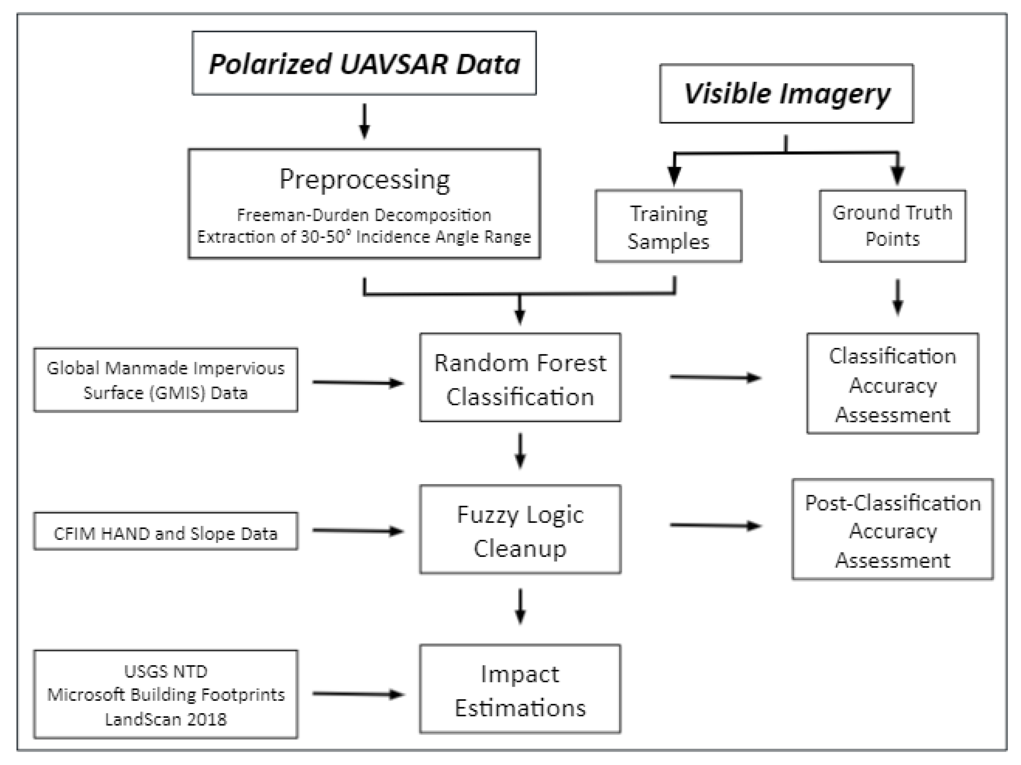
The ancillary datasets used in this study were chosen for their statistical information about the study area, from land cover type and elevation to urban development level and population distribution. These sources provide supplementary information that is challenging or impossible to derive from UAVSAR and/or visible data alone. Implemented at various stages of the workflow presented in Figure 3, ancillary datasets play a critical role in postclassification refinement and impact estimations.
The NLCD 2016 is a reliable, high-resolution land cover reference for the contiguous U.S. The dataset offers a 30 m resolution estimation of 16 land cover types derived from Landsat and ancillary data [22]. NLCD 2016 values were used to estimate the area-proportional number of training and ground truth points needed for classification.
The NASA Socioeconomic Data and Applications Center (SEDAC) hosts the Global Manmade Impervious Surface (GMIS) dataset, a similar Landsat visible reflectance-derived estimate of fractional impervious land cover with 30 m global coverage [42]. The Global Manmade and Impervious Surface (GMIS) dataset is incorporated as a classification feature to reduce potential sources of confusion between inundated and noninundated areas. Urban samples were taken from areas of high imperviousness, with percentage values near 100%. Water and inundated samples, all taken from the center of water bodies or wetlands, have impervious values near 0%. This variation aids in class determination when backscatter signatures for the different classes are similar.
Oak Ridge National Laboratory operates the Continental Flood Inundation Mapping (CFIM) data repository, containing hydraulic properties for 2.7 million river catchments across the contiguous U.S. [43]. The repository uses ORNL’s high-performance computational framework to derive Height Above Nearest Drainage (HAND) using 10 m USGS National Elevation and National Hydrography Dataset Plus (NHDPlus) hydrologic data. The HAND model was introduced by Nobre et al. (2011) as a method for normalizing topography relative to its drainage network to estimate local water table depth and drainage potential [44]. The topographic slope of each pixel is generated using methodology outlined by Tarboton (1997), which calculates the steepest outward slope on one of eight triangular facets centered at each grid cell. This method reports the drop in elevation over distance, or inverse tangent of the slope angle, and requires an arctan conversion to derive the slope angle used in analysis [45]. HAND and slope raster data for the Lumber and Cape Fear River basins were incorporated into a fuzzy logic model for postclassification refinement of detected open-water and inundated forest pixels.
The USGS National Transportation Dataset is based on TIGER/Line data provided by the U.S. Census Bureau supplemented with HERE Technologies road data to generate maps of roads, railroads, trails, airports, and other transportation features [18]. This dataset enables the estimation of flooding impacts on roadways, which is evaluated based on the location and extent of affected thoroughfares.
In 2018, Microsoft released a machine learning-based building footprint dataset that includes over 125 million buildings in all 50 US states in GeoJSON format. This dataset was produced using labeled images from Bing imagery and the Open-Source Microsoft Cognitive Toolkit (CNTK) [17]. Rasterized building footprints are used to estimate impacts following classification.
Oak Ridge National Laboratory’s LandScan is the finest-resolution global population distribution data publicly available and represents an area’s average population over 24 h. The LandScan algorithm provides a 1 km view of tabular Census data by incorporating imagery analysis technologies, spatial data, and a multivariable dasymetric modeling approach [16]. Population information is used to estimate the level of societal impact in localities affected by flooding.

3. Methods

3.1. Random Forest Classification

3.1.1. Class Determination and Training Sample Gathering

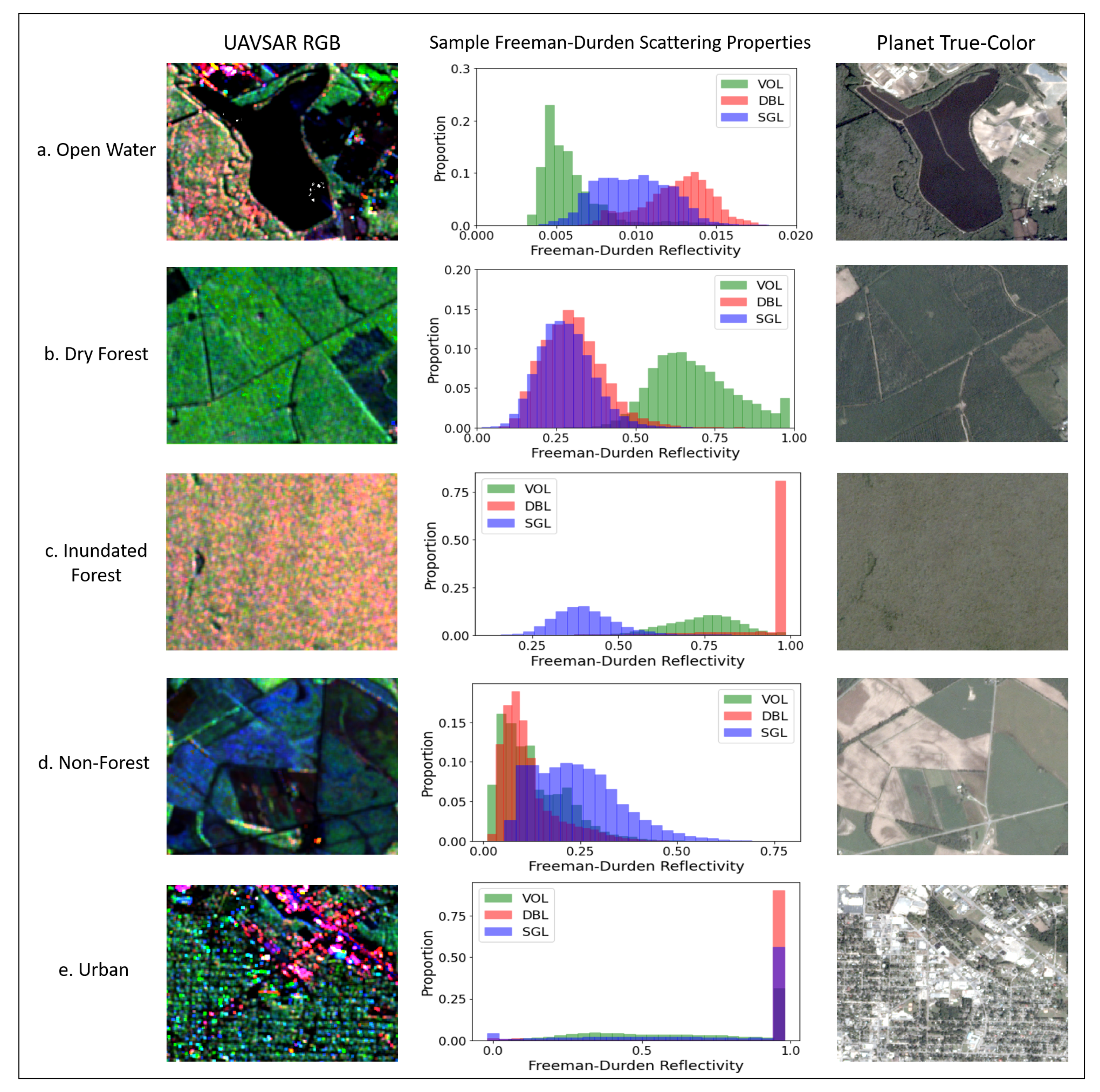
As noted in Section 2.1, forested and agricultural areas comprise a majority of the study area. The focus of this analysis on flooding motivated the designation of the open water and inundated forest classes. To account for the remaining types of land cover, classes for dry forest, nonforest, and urban areas were developed. These classes were chosen through an iterative process focused on maximizing classifier skill in the focus classes of open water and inundated forest. Each class has a distinct backscatter signature, as visualized in Figure 4. The sampled scattering mechanisms are expected to be ubiquitous to similar land cover types and scenarios; therefore, some amount of skill is anticipated when the model is applied to similar environments.
The distributions of single, double, and volume scattering intensities for the training samples of each class are also demonstrated in Figure 4. Open water is characterized by extremely low backscatter in all three scattering types, with single, double, and volume scattering contributions ranging from 0.003 to 0.18. In some instances of specular reflection, backscatter is very close to zero. These values are rounded down during the preprocessing steps and result in apparent data gaps over some of the larger water bodies in the region.
Volume scattering strongly dominates in dry forest areas due to canopy interactions with the radar beam. Single and double-bounce scattering occurs at each peak near 0.25 and 0.3, respectively (Figure 4). When inundation is present beneath the canopy, the dominant scattering mechanism changes to double-bounce, as noted in previous studies [3,5,8]. This shift in double-bounce scattering proportion is clearly identifiable in the histograms for the inundated and dry forest classes. The enhanced double-bounce signature exhibited by floodwaters present beneath the canopy gives inundated pixels a unique scattering signature. Pixels containing inundation typically have average values near 160 for red, 83 for green, and 46 for blue, which stand out as hues of orange and pink in the false-color RGB (Figure 4).
Nonforest samples were taken from areas of bare soil or short or sparse vegetative cover, which can exhibit similar scattering signatures to water. Though there is no observable surface water in these areas, brightening due to the enhanced soil moisture can be observed [36]. The sensitivity of UAVSAR to soil moisture allows it to capture a darkening trend as soils incrementally dry each day, visualized by the contraction of the plotted intensity distributions toward zero in Figure 5. Over the five-day period, the single and double-bounce backscatter are reduced to near-zero over nonforest pixels, overlapping with the range of observed values of water samples. This overlap indicates the potential for misclassification given the similar training values associated with two separate classes. In an attempt to mitigate some of this confusion, sample pixels were extracted from the same areas on two days, 19 and 23 September, to capture conditions near peak flood and at a relatively lower water extent.
The urban class represents another opportunity for misclassification, given the wide range of backscatter values it represents. This is due to the diversity of ‘urban’ features: roads, parking lots, commercial and residential buildings, and solar panel farms, all of which have different scattering properties. Urban inundation classification in the Lumberton, NC area following Hurricane Matthew (2016) using C-band Sentinel-1 was performed by Lin et al. (2019). Asphalt surfaces and shadow effects were major sources of flood underprediction in urban areas. Smooth paved surfaces exhibit backscatter signatures similar to water, making them indistinguishable from flooded areas in most cases [36]. Likewise, the potential exists for confusion between the urban and inundated forest classes due to their characteristic double-bounce scattering, especially when buildings are oriented perpendicular to the instrument’s flight path [5].
As the actual land cover of a pixel cannot be consistently and accurately determined from SAR data alone, Planet visible imagery is used as a reference. Thus, the collection of training samples is limited to areas with overlapping visible and UAVSAR coverage. Allocation of training pixels followed suggested practices outlined in Colditz (2015), which recommends area-proportional sample allocation and a total sample area equivalent to 0.25% of the total image area [46]. Samples are taken from a single swath (LT1) to train the RF classifier, which is then implemented on the remaining data swaths to minimize user input. The proportional area of each sample class was estimated using reclassified NLCD 2016 values as a proxy. An example of the allocation of training pixels per class is outlined in Table 1. This method assumes that all wetland areas are inundated, though there are likely inundated non-wetlands and dry wetland pixels present in the image. However, given the specificity of the UAVSAR observations to this flood event, NLCD 2016 is the closest truth proxy available.

3.1.2. Classification and Accuracy Assessment

The RF classification performed utilizes the scikit-learn Python module, which provides state-of-the-art machine learning algorithms for use in both supervised and unsupervised classifications [47]. Decision tree classifiers such as RF do not assume a particular data distribution, making them well suited for SAR applications [11,48]. RF uses a bootstrap aggregating approach, randomly sampling training data with replacement. Since each sample is replaced, it is possible to select the same data multiple times while other data is unused. This method makes the classifier more robust to random variations or noise and resistant to overfitting [11,13]. A train/test split of 0.7/0.3 was used to calibrate the RF classifier, meaning that 70% of sampled pixels were used to train the classifier while the remaining 30% were used to assess its performance. The parameters at which the classifier achieves maximum accuracy can be determined using scikit-learn’s built-in validation curve function, which indicates that the classifier quickly reaches optimal performance, stabilizing after about ten trees. This motivated the number of trees to be set at 20. Additionally, while the default option allows trees to grow fully, the trees in this classifier are pruned at a maximum depth of ten for computational efficiency. A similar validation curve for maximum depth demonstrates that increases in classifier performance were negligible after ten. Default values were used for the remaining hyperparameters.
A statistical assessment of the classifier’s accuracy is performed by comparing the predicted land cover class to the class value of manually identified ground truth points. The recommended accuracy assessment practices outlined in Olofsson et al. (2014) include a stratified random sampling method, which allocates truth points to classes based on their proportional area [15]. This allocation follows a method introduced by Cochran (1977) that incorporates the user-desired standard error of overall accuracy, S(O), the proportional area of class i ( W i ), and the standard deviation of stratum i, S i = U A i ( 1 U A i ) [15]. Since the calculated target number of truth points (n) is dependent on the user-chosen overall standard error and user accuracy ( U A i ) for each class, it is suggested that the calculations be performed several times with a variety of input values (Equation (1)) [15]. The focus on flooding for this study motivated the selection of 0.8 for open-water UA, 0.9 for inundated forest UA, and 0.75 for the UA of the remaining classes. Additionally, an overall standard error of 1.5% was selected.
n = W i S i S ( O ) 2
The calculations performed by Olofsson et al. (2014) are based on a pixel resolution of 30 m, approximately five times coarser than the UAVSAR resolution of ∼6 m. To account for this difference, the calculated target number of truth pixels for each class is divided by five. This adjustment results in about 4200 truth pixels for each of the fifteen data swaths. Similar to training samples, ground truth pixels are assessed in areas with overlapping UAVSAR and visible coverage, which vary on a daily basis depending on satellite overpasses, aerial flight tracks, and cloud cover. The extent of flooding also varied daily as waters drained and crests moved downriver. These factors required ground truth pixels to be updated daily to maintain their validity. This verification process relies on the availability of cloud-free optical data, and the manual identification of land cover classes is exceedingly time-intensive. To account for these limitations, randomly-distributed ground truth points were buffered by 10 m to collect groups of pixels rather than individual ones. The resulting target value near 420 points per swath was more feasible for the time constraints limiting this study. An example of the truth pixel allocation for a single flight track is displayed in Table 2.
The accuracy metrics reported for the RF-generated land cover maps include the overall accuracy, user’s accuracy (commission error), and producer’s accuracy (omission error) [15]. Overall accuracy (OA) is given by dividing the sum of correctly classified points for each class (up to q classes) by the total number of points (p) (Equation (2)).
O A = j = 1 q p j j
User’s accuracy is calculated for each class and demonstrates the percentage of points with output class i and reference class i (Equation (3)). High values of UA indicate a low amount of overprediction, or false-positives, while low values signal significant overprediction [36].
U A i = p i i p i
Conversely, the producer’s accuracy (PA) demonstrates the percentage of points with reference class j and output class j (Equation (4)). High values of PA indicate a low amount of underprediction, or false negatives, while low values signal significant underprediction [36].
P A j = p j j p j
The OA, UA, and PA for each iteration are reported by class in confusion matrices, cross-tabulations of the class labels assigned by the RF classifier against ground truth pixels. The matrix rows represent the RF classifier determinations, and the columns represent the ground truth point class labels [15]. Confusion matrices were generated for each RF classification iteration to assess accuracy before fuzzy logic cleanup operations. After postclassification steps, UA and PA metrics are reassessed for the individual and combined extent (“Floodmap”) of the open-water and inundated forest classes. Partners from FEMA have requested a product accuracy of at least 80% within 48 h of impacts [49]. Therefore, OA, UA, and PA values of 80% or higher are considered satisfactory.

3.1.3. Post-Classification

The resulting classified image contains small noise-like features and some obvious misclassifications. To reduce false detections and generate a more continuous and realistic output, fuzzy logic cleanup operations are performed using scikit-fuzzy, a robust fuzzy logic toolkit for SciPy [50]. Defined by Zadeh (1965), a fuzzy set is characterized by a membership function which assigns each object a 0–1 membership value [51]. Fuzzy logic combines information from various sources and accounts for uncertainty through membership rather than binary classes [52].
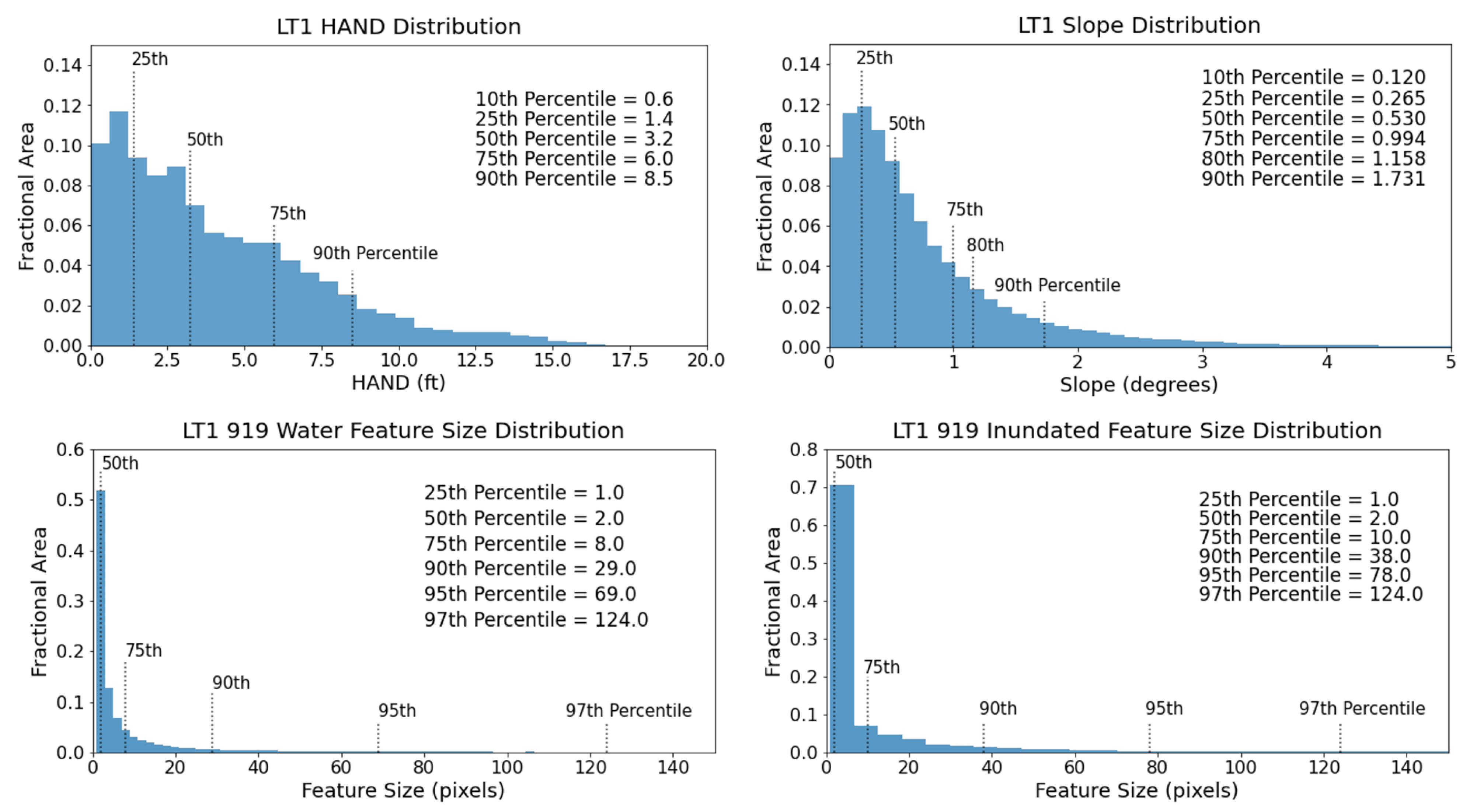
The fuzzy logic technique is used in Martinis et al. (2015) to refine SAR-derived inundation based on pixel elevation, slope, backscatter power, and contiguous feature area. Given the inclusion of SAR backscatter in the RF classification workflow, that element is omitted in the fuzzy logic scheme used here. ORNL-CFIM HAND and slope are incorporated to reduce false detections in elevated areas unlikely to be flooded. The contiguous areas of classified water and inundated pixels are also used to reduce the number of small lookalike features [52]. A standard Z function is used to determine membership degrees of features above and below user-defined thresholds [51]. This function uses a polynomial curve to assign 0–1 degrees of membership to input values which allows a transition between pixels deemed flooded/not flooded. Values of HAND, slope, and feature area below minimum thresholds are assigned membership values of zero, while those above the maximum threshold have membership values of one. These thresholds were set according to statistical margins decided after several trials aimed at maximizing the benefits and minimizing the costs of this fuzzy logic cleanup method on the final flood map accuracy. For HAND, the 50th to 75th percentiles are used as minimum and maximum thresholds. These thresholds are 50–80th percentile for slope and 95–97th percentile for area. Example distributions of each of the elements used in this fuzzy set are visualized in Figure 6.
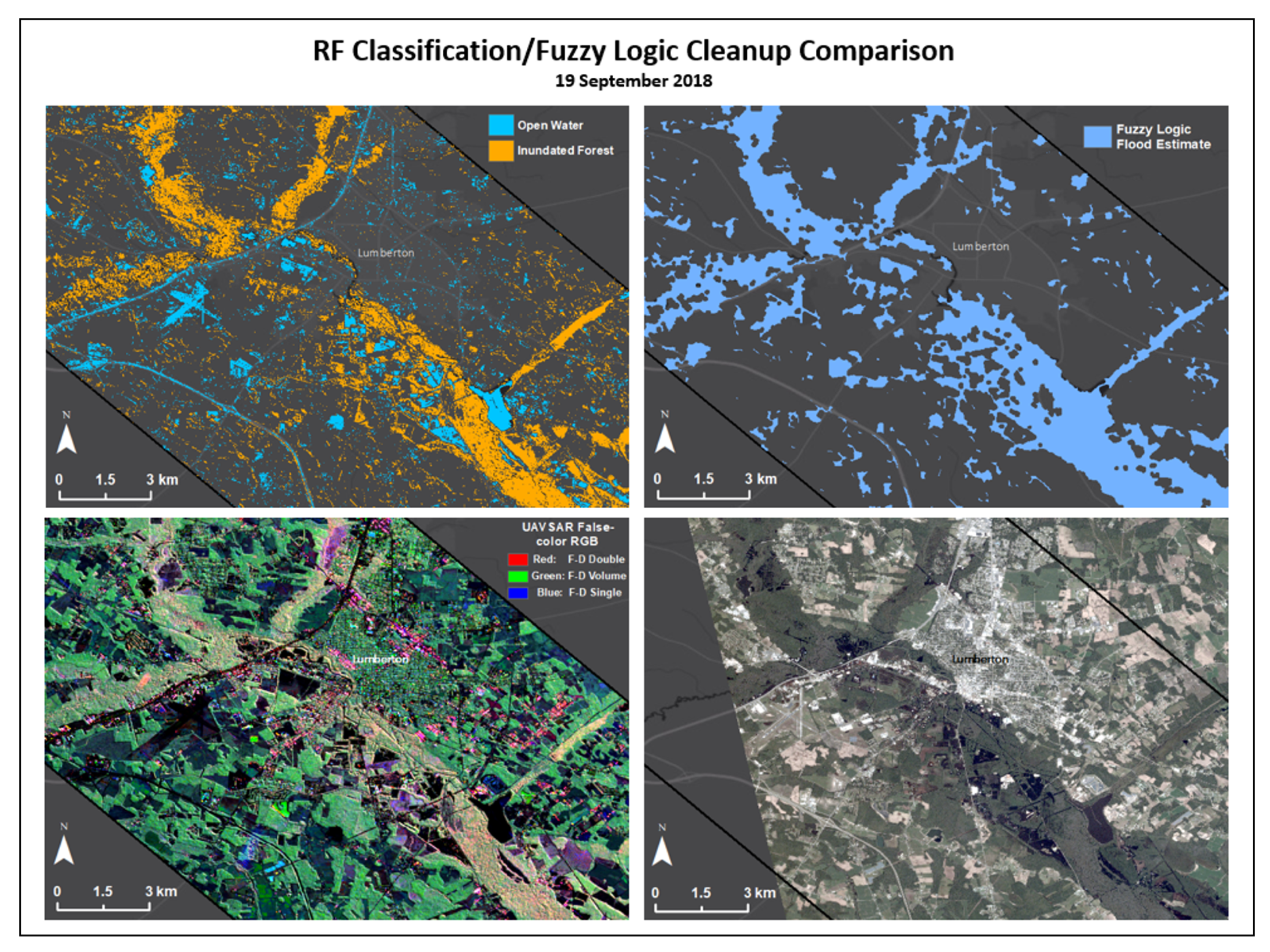
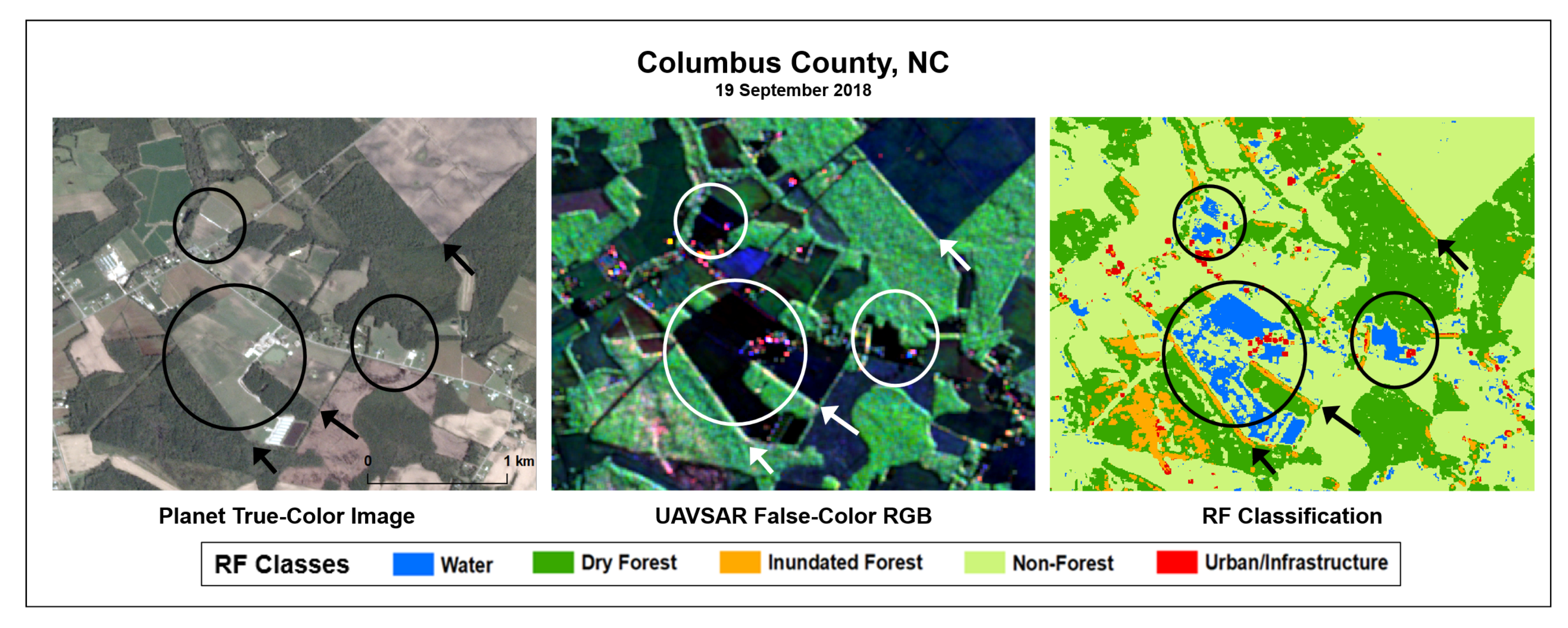
The fuzzy elements are combined into a composite set by averaging the membership degrees of each pixel. A further “defuzzification” step is performed by masking pixels with combined membership degrees of <0.85 [52]. This membership threshold was increased from 0.65 to account for the upward shift in membership degrees attributed to the large expanses of flat and low-lying areas in this region. The fuzzy logic scheme is implemented on the water and inundation classes separately before the two are merged into a single flood extent. Lastly, a morphological closing process is performed using scikit-image to fill small gaps between features classified as water and inundated, generating a more continuous flood map raster. Figure 7 demonstrates a comparison between the RF classification results and the flood map derived from them through fuzzy logic and morphological closing.

4. Results

4.1. RF Classification

The RF classification was implemented on a total of fifteen UAVSAR data swaths over four flight tracks sampled during the 18 to 23 September 2018 observation period. Confusion matrices were developed for each classification output to derive user, producer, and overall accuracies for each class. Results are reported in daily averages and a comprehensive event average across all fifteen classified images is shown in Table 3 for conciseness. The average overall RF classification accuracy was 87.67%, with a daily maximum of 89.37% on 20 September and a minimum of 86.36% on 18 September. These values indicate relatively low amounts of under- and overprediction, demonstrating the ability of the RF algorithm to capture the temporal evolution of the flood with a relatively steady level of skill.
Additionally, the average OA for each date and flight track exceeds the FEMA target of 80% [49]. The focus classes of open water and inundated forest also demonstrate average UA and PA values above 80%. These results are consistent with Huang et al. (2021), a machine learning-based inundation detection effort utilizing UAVSAR data collected over irrigated croplands. In this study, an overall RF classification accuracy of 87.62% was attained using the Freeman–Durden decomposition and ancillary vegetation data. Inundation in rice fields was detected with a UA and PA of 86.35% and 74.85%, respectively [30].
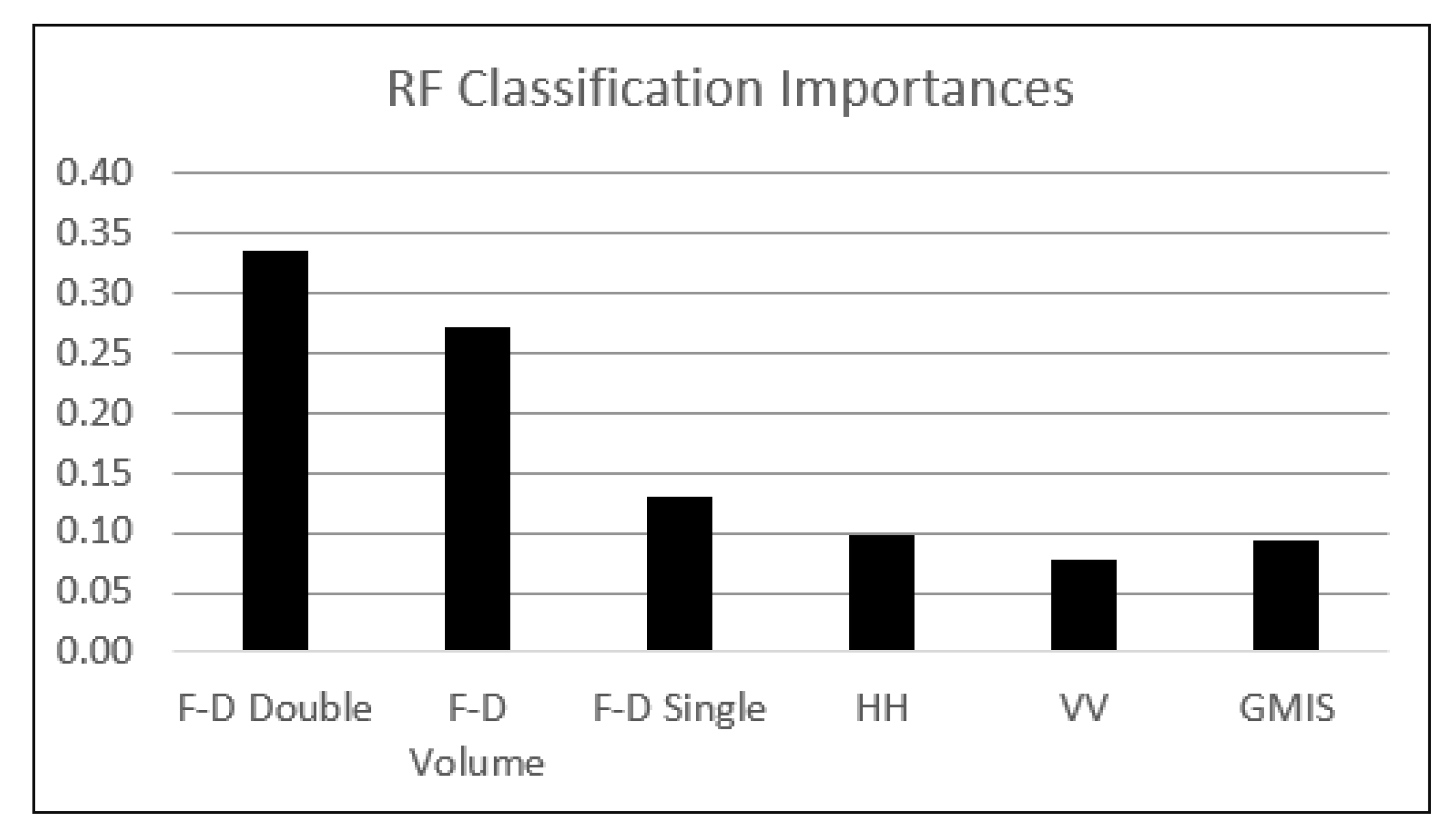
The scikit-learn RF algorithm uses a unitless Gini Index to estimate the importance of input features used in the decision-making process by measuring the decrease in accuracy observed from removing each element [47]. The Freeman–Durden scattering mechanisms are shown to have the most value in class determination. Double-bounce and volume scattering demonstrate a significant amount of added skill compared to the other features used in this analysis, given their importances greater than 0.25 (Figure 8). Single scattering is the third most important at 0.13, followed by HH, GIMS percentage, and VV at 0.10, 0.09, and 0.08, respectively.

4.2. Post-Classification

The feature size fuzzy element effectively reduces the number of small noise-like water and inundated pixels and helps the interpretability of the flood map. However, this element also removes accurate observations limited in size due to data artifacts or misclassifications, which decreases the water PA by an average of 11%, denoted in Table 4. The morphological image closing step adds some of these features back to the flood extent (Figure 7). Unfortunately, it also works to increase the size of falsely detected water features, compounding some areas of overprediction that remain after the fuzzy logic process. This is reflected in the significant decrease of 62% in average open-water UA after postclassification.
The inundated forest class showed an increase in PA (or reduction in underprediction) of 4%, attributed to the elimination of small discontinuities in the flood extent. Seven out of the fifteen classified maps obtained an inundated PA greater than 95%, and one reached 100%. Some larger gaps remain in areas with significant urban misclassification or other spaces too large to be filled in the image closing step. Areas of misclassification such as these prevent a higher PA in the remaining maps. An increase in overprediction is observed because more prominent edge artifacts are kept during the fuzzy logic process due to their size. This results in a postclassification decrease in inundated UA of 24%, a significant but smaller reduction than that of the open-water class UA.

4.3. Societal Impacts

The estimation of impacts on buildings, roads, and people was complicated by discontinuities and false detections in the estimated flood extent. Impacts were calculated by aggregating the daily flood extents for each flight track into an event maximum and intersecting the ancillary datasets. This approach offers a rough summary of impacts for the entire event comparable to the damage assessments currently performed operationally. In total, an estimated 11,618 buildings and 6118 roads and road segments were impacted by flooding across the study area during the 18 to 23 September observation period. Given the comparatively coarse resolution of the LandScan 2018 dataset, population impacts are expressed as an approximation of people within 1 km of detected flooding. The resulting estimate of 365,853 people, or about 79% of the area’s population, is assumed to be a significant overestimation due to the large resolution difference between LandScan and the other datasets used for analysis.
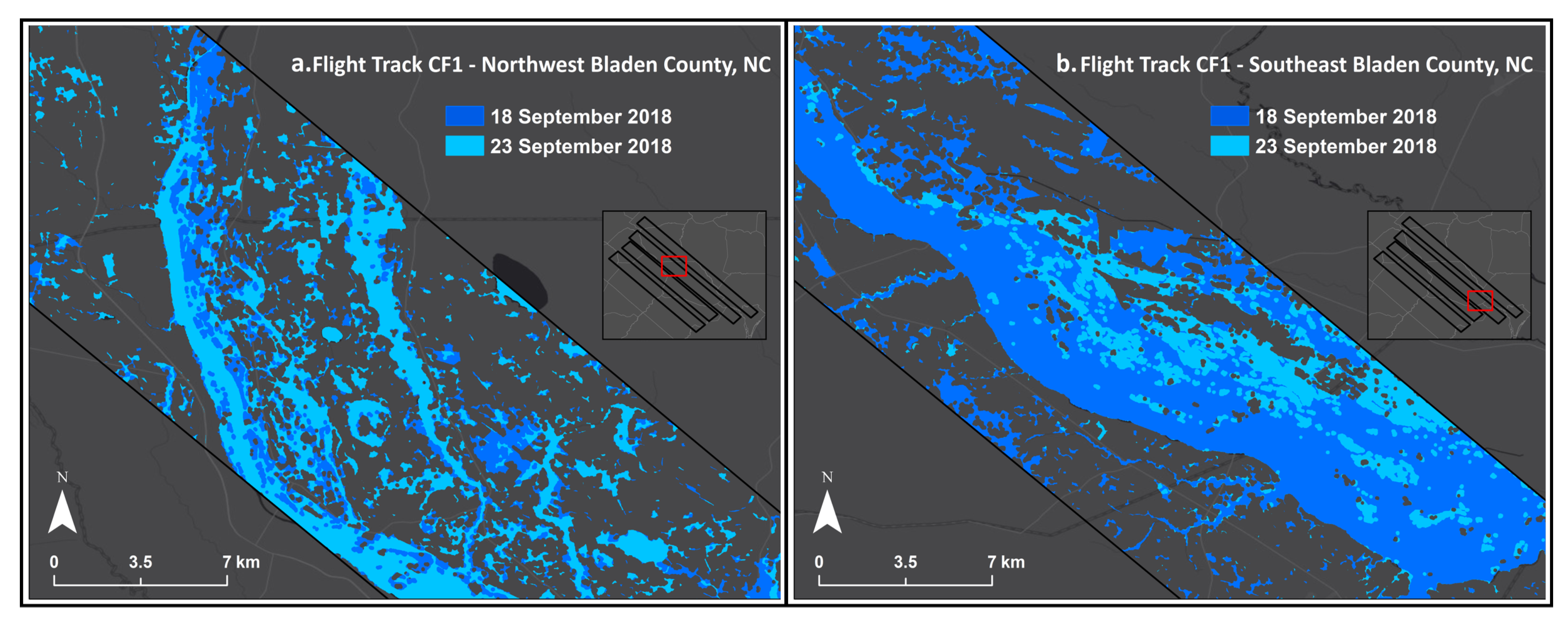
The repeated UAVSAR observations capture the temporal evolution of the flood extent. Some inaccessible areas on 18 September are no longer inundated after just a few days, while others remain flooded for the entire observation period. This is visualized in Figure 9, which depicts the downstream shift of flooding along the Cape Fear River in Bladen County, NC. Northwestern portions of the county experienced a decrease in inundation over the observation period (Figure 9a), while the opposite is true for areas in southeast Bladen County (Figure 9b). For water-damaged structures, remediation actions are extremely time-sensitive given the human health risks associated with mold. Daily observations may support these actions by providing indications of where floodwaters are receding and damaged routes and structures are becoming accessible to response personnel.

5. Discussion

5.1. Classifier Performance

5.1.1. Areas of Underprediction

The open-water class suffered from underprediction due to enhanced backscatter caused by several phenomena. Water surface roughening due to wind is a common source of error in SAR-based water detection [5,53]. Ripples and waves caused by the wind generate Bragg resonance, which increases backscatter as a function of wind speed and direction with respect to the radar viewing angle [54]. This type of wind-induced misclassification is evident across several large, permanent water bodies within the region. Classifier confusion generated by waves on water surfaces is a well-documented limitation of water-mapping activities using SAR [3,9]. These areas of confusion disproportionately impact the open-water UA because a majority of the ground truth points are taken from such permanent water bodies.
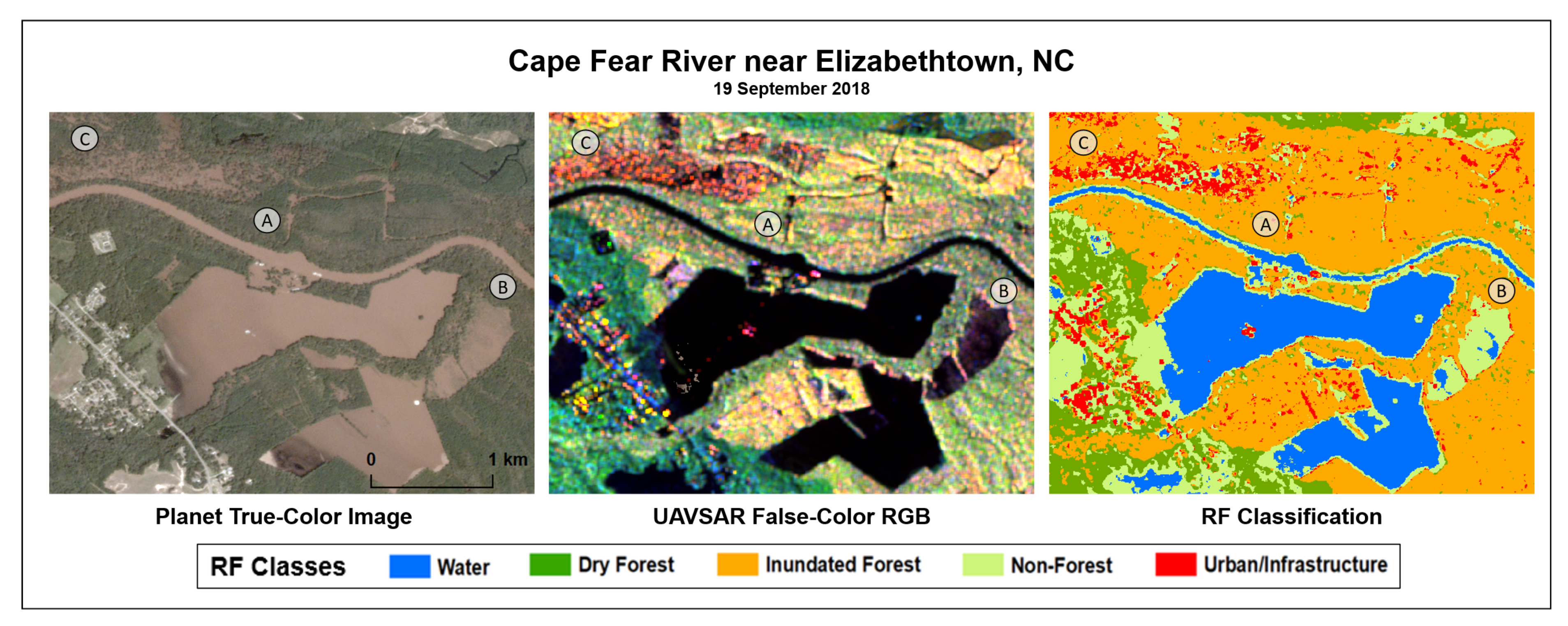
The edges of detected water features are another source of underprediction, attributed to inherent layover and shadow effects present in side-looking SAR systems such as UAVSAR [36]. Figure 10A shows that the detected water pixels of the Cape Fear River and overbank flooding are surrounded by “dry” nonforest pixels, underestimating the water extent. Conversely, vertical objects oriented parallel to the UAVSAR flight track reflect a significant amount of energy back to the sensor and can create bright artifacts larger than the number of pixels the structure occupies in reality. The scattering signature from a single building within the expansive flooded area south of A is an example of underprediction stemming from a bright feature. Urban flood detection with SAR continues to be a challenge because of the complex mosaic of backscatter intensities generated by a high density of features such as trees and buildings [5,36,53].
Figure 10B highlights another source of confusion between the open-water and nonforest classes. Variation in soil moisture levels or water depth can change the backscatter signature of features and impact the ability to discriminate between flooded and nonflooded areas [27]. The impact of vegetation on backscatter is a function of both plant height and inundation depth. Pulvirenti et al. (2011) observed that emergent plant stems can enhance backscatter until they become too submerged to produce significant double-bounce scattering [53]. Visible imagery suggests that the fields to the southwest of the marker are flooded, with vegetation partially or entirely submerged. Underprediction, such as in Figure 10B, is prominent in rural and agricultural areas which feature expanses of crops or grasses at varying stages of growth.
The inundated class encountered issues with underprediction due to brightness and shadow artifacts. Spaces between trees larger than one or two pixels allow double-bounce scattering to dominate, creating similar signatures to those produced by buildings and other vertical structures. This causes some inundated areas to be falsely classified as urban, as demonstrated by Figure 10C. While the difference between these areas of inundated forest and the developed portion to the south is evident in true-color imagery, their structural similarities generate very similar SAR backscatter signatures.

5.1.2. Areas of Overprediction

Overprediction of open water was significant in urban areas. Paved surfaces such as airport runways and interstate highways exhibit specular backscatter akin to water surfaces. The similar reflective properties of paved surfaces to water have been noted as a limitation to urban flood detection using SAR by several studies [5,36,53]. Specular reflection also caused numerous false water detections over expanses of bare soils and patchy or short vegetation, such as the circled areas in Figure 11. In many of these fields, there is no water visible on the surface. Bare soils and plants at an early growth stage have been shown to exhibit backscatter similar to water in flooded conditions [53].
False detections of inundation were numerous among tree stands with edges parallel to the UAVSAR flight track. These linear features are generated by the almost pure double-bounce scattering produced by the vertical extent of trees bordering the flat surfaces of fields or water, and are indicated with arrows in Figure 11. Misclassifications also occurred in forest clearings with saturated soils. The area of these false inundation detections remains relatively steady over the observation period, in contrast to the varying daily extent of accurately classified inundation.

5.2. Comparison to Current Operational Product

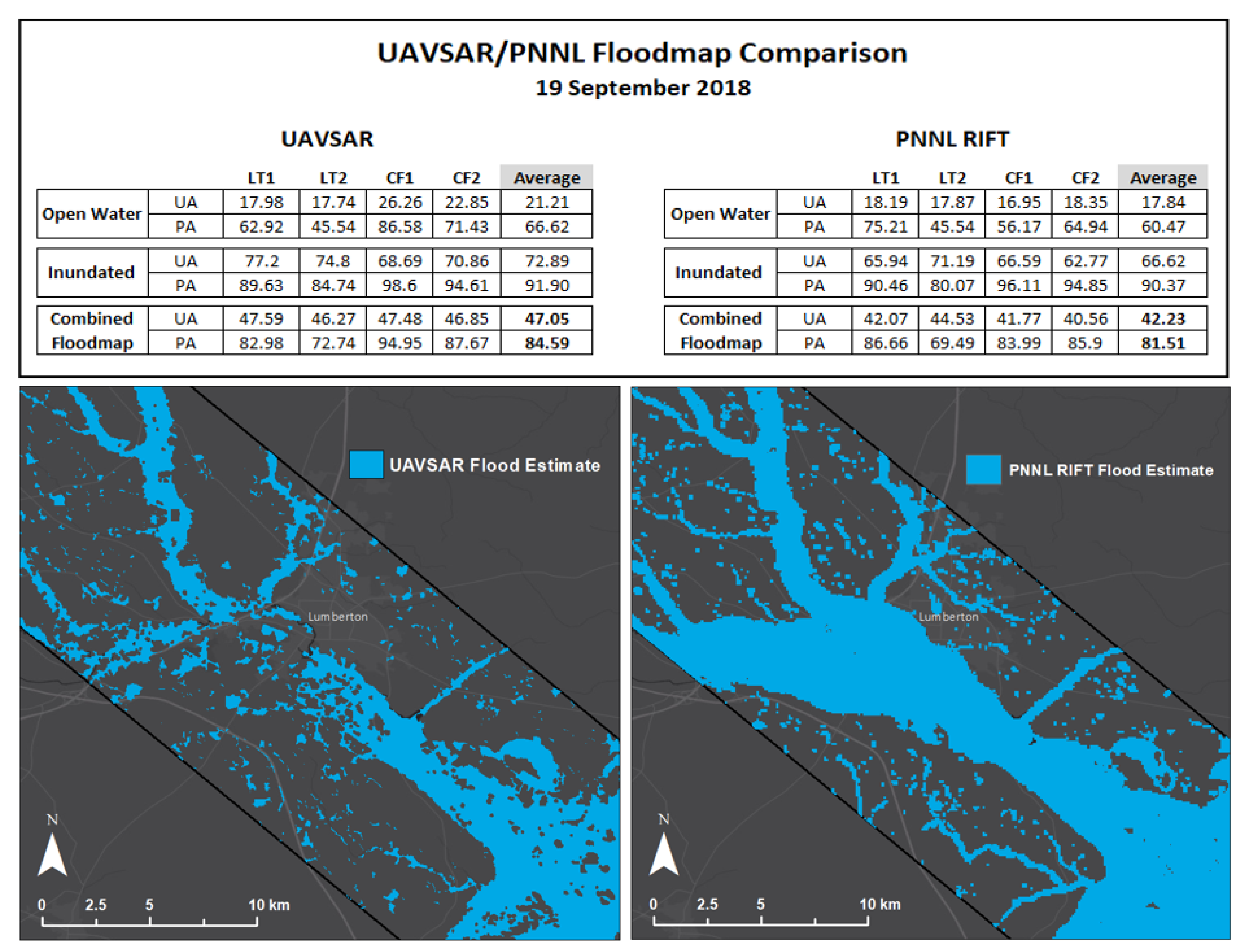
The NASA Earth Science Disasters program has recently partnered with emergency management personnel from the North Carolina Department of Public Safety (NC DPS). This partnership aims to assess the current flood estimation products used in emergency response situations, such as hurricane landfalls, and offers supplementary remote-sensing products. Currently, the NC DPS uses flood estimates generated by the Rapid Infrastructure Flood Tool (RIFT) developed by Pacific Northwest National Laboratory (PNNL). This hydrodynamic model generates 90 m resolution flood extents and depths based on simulated or observed rainfall and is distributed by the FEMA Mapping and Analysis Center (MAC) [55].
To compare the skill level of the UAVSAR-derived flood extent to the PNNL RIFT model output, estimations for 19 September 2018 from both sources are tested against the ground truth points (outlined in Section 3.1.2) for that date. Flood detections by PNNL RIFT outside of the UAVSAR processing areas are masked to isolate the analysis to areas of overlapping coverage and truth data. Figure 12 contains a visualization of the two flood estimates over a subset containing the city of Lumberton, NC. The accuracy statistics for each map is calculated over the entire flight track. The UAVSAR-derived flood map has a UA of 47.05% and PA of 84.59%. The PNNL RIFT map demonstrates slightly lower user and producer accuracy values of 42.23% and 81.51%, respectively. This limited analysis suggests that UAVSAR-derived flood extents have a comparable or slightly higher level of accuracy to the rapid response products currently being used by the NC DPS. It also shows that overprediction is a significant source of error for other methods of estimating flood extent, and suggests the results demonstrated from this methodology are comparable to currently operational products. It should be noted that the PNNL RIFT model displays the maximum possible extent of water based on observed precipitation and ground elevation, irrespective of manmade structures. Conversely, the UAVSAR map is produced using instantaneous observations of the ground, which includes all buildings and structures present. These features are classified as ‘urban’ and are omitted from the final flood map, resulting in the large difference in the estimated inundation extent around the city seen in Figure 12. Though it is hard to directly compare the varying estimates, both methods can provide crucial information for response activities.

6. Conclusions

This study demonstrated the unique capabilities of L-band SAR that make it a potentially reliable source of inundation detection in forested or vegetated areas. Using Hurricane Florence of September 2018 as a case study, an RF classification scheme was developed based on L-band UAVSAR and ancillary datasets. This methodology produced skillful class determinations with training data limited in spatial and temporal availability. A consistent average overall RF classification accuracy above 85% was achieved for the fifteen UAVSAR data swaths gathered over southeastern North Carolina. The results of the RF classification suggest a high level of skill in detecting inundated vegetation, while open-water estimation is somewhat limited by confusion with similar land surface types. The inundated forest class showed average user and producer accuracies of 94.91% and 89.78%, respectively. The open-water class exhibited an average user accuracy of 85.65% and producer accuracy of 82.14%.
Following the RF classification, pixels from these two classes were combined and refined into a more contiguous flood extent using fuzzy logic. This postclassification method maintains a high average producer accuracy (87.15%) while significantly reducing the average user accuracy to 46.96%, indicating considerable overprediction of flooding. Underprediction is notable in dense urban areas, limiting the estimation of societal impacts in more populated locales. Validating data for these estimations is also extremely limited. Despite relatively lower accuracies than the RF output, a postprocessed flood map is demonstrated to have comparable skill to the PNNL RIFT hydrological model for observations taken on 19 September 2018. The classification and postclassification processes shown in this study can be implemented daily as UAVSAR (and later, NISAR) data becomes available, making it useful in real-time response situations. The L-band SAR-derived flood estimate can be used to supplement hydrological model outputs and provide observations where visible and near-IR imagery is unavailable, increasing the amount of information available to emergency responders. Future efforts will explore other methods of polarimetric decomposition and machine learning techniques. Additionally, the applicability of this model to other regions and flood events will be assessed.

Author Contributions

This article is adapted from the M.S. thesis work of A.M.M., A.L.M., R.E.G. and J.R.M. served as committee members, while L.A.S. and J.R.B. provided invaluable expertise and instruction crucial to the completion of this study. Conceptualization, A.L.M. and J.R.M.; data curation, A.M.M. and A.L.M.; formal analysis, A.M.M.; funding acquisition, A.L.M.; investigation, A.M.M.; project management, A.L.M. and L.A.S.; methodology, A.M.M., A.L.M., L.A.S. and J.R.B.; resources, A.L.M., R.E.G. and J.R.M.; software, A.L.M., L.A.S. and J.R.B., supervision, A.L.M. and L.A.S.; validation, A.M.M., L.A.S. and J.R.B.; visualization, A.M.M.; writing—original draft preparation, A.M.M.; writing—review and editing, A.L.M., R.E.G., J.R.M., L.A.S. and J.R.B. All authors have read and agreed to the published version of the manuscript.

Funding

This research was funded by the NASA Earth Science Disasters Program through NASA Cooperative Agreement NNM11AA01A.

Conflicts of Interest

The authors declare no conflict of interest.

References

  1. NOAA National Centers for Environmental Information (NCEI) U.S. Billion-Dollar Weather and Climate Disasters. Available online: https://www.ncdc.noaa.gov/billions/summary-stats (accessed on 27 April 2021).
  2. National Research Council. Benefits and Costs of Accurate Flood Mapping. In Mapping the Zone: Improving Flood Map Accuracy; The National Academies Press: Washington, DC, USA, 2009; pp. 79–80. [Google Scholar]
  3. Martinez, J.; Le Toan, T. Mapping of Flood Dynamics and Spatial Distribution of Vegetation in the Amazon Floodplain using Multitemporal SAR Data. Remote Sens. Environ. 2007, 108, 209–223. [Google Scholar] [CrossRef]
  4. NASA Applied Remote Sensing Training (ARSET) Program: Introduction to Synthetic Aperture Radar. Available online: appliedsciences.nasa.gov/join-mission/training/english/arset-introduction-synthetic-aperture-radar (accessed on 7 June 2019).
  5. Chapman, B.; McDonald, K.; Shimada, M.; Rosenqvist, A.; Schroeder, R.; Hess, L. Mapping Regional Inundation with Spaceborne L-Band SAR. Remote Sens. 2015, 7, 5440–5470. [Google Scholar] [CrossRef] [Green Version]
  6. Meyer, F. Spaceborne Synthetic Aperture Radar—Principles, Data Access, and Basic Processing Techniques. In SAR Handbook: Comprehensive Methodologies for Forest Monitoring and Biomass Estimation; Flores, A., Herndon, K., Thapa, R., Cherrington, E., Eds.; SERVIR Global Science Coordination Office: Huntsville, AL, USA, 2019; pp. 26–30. [Google Scholar]
  7. Wang, Y.; Hess, L.; Filoso, S.; Melack, J.M. Understanding the Radar Back-Scattering from Flooded and Nonflooded Amazonian Forests: Results from Canopy Backscatter Modeling. Remote Sens. Environ. 1995, 54, 324–332. [Google Scholar] [CrossRef]
  8. Richards, J.A.; Woodgate, P.W.; Skidmore, A.K. An Explanation of Enhanced Radar Backscattering from Flooded Forests. Int. J. Remote Sens. 1987, 8, 1093–1100. [Google Scholar] [CrossRef]
  9. Ramsey, E.; Rangoonwala, A.; Bannister, T. Coastal Flood Inundation Monitoring with Satellite C-band and L-band Synthetic Aperture Radar Data. J. Am. Water Resour. Assoc. 2013, 49, 1239–1260. [Google Scholar] [CrossRef]
  10. Belgiu, M. and Dragu, L. Random Forest in Remote Sensing: A Review of Applications and Future Directions. ISPRS J. Photogramm. Remote Sens. 2016, 114, 24–31. [Google Scholar] [CrossRef]
  11. Brieman, L. Random Forests. Mach. Learn. 2001, 45, 5–32. [Google Scholar] [CrossRef] [Green Version]
  12. Du, P.; Samat, A.; Waske, B.; Liu, S.; Li, Z. Random Forest and Rotation Forest for Fully Polarized SAR Image Classification using Polarimetric and Spatial Features. ISPRS J. Photogramm. Remote Sens. 2015, 105, 38–53. [Google Scholar] [CrossRef]
  13. Rodriguez-Galiano, V.; Ghimire, B.; Rogan, J.; Chica-Olmo, M.; Rigol-Sanchez, J. An Assessment of the Effectiveness of a Random Forest Classifier for Land Cover Classification. ISPRS J. Photogramm. Remote Sens. 2012, 67, 93–104. [Google Scholar] [CrossRef]
  14. Uhlmann, S. and Kiranyaz, S. Integrating Color Features in Polarimetric SAR Image Classification. IEEE Trans. Geosci. Remote Sens. 2014, 52, 2197–2206. [Google Scholar] [CrossRef]
  15. Olofsson, P.; Foody, G.M.; Herold, M.; Stehman, S.V.; Woodcock, C.E.; Wulder, M.A. Good Practices for Estimating Area and Assessing Accuracy of Land Change. Remote Sens. Environ. 2014, 148, 42–57. [Google Scholar] [CrossRef]
  16. Rose, A.N.; McKee, J.J.; Urban, M.L.; Bright, E.A.; Sims, K.M. Oak Ridge National Laboratory LandScan 2018 Global Population Database. Available online: https://landscan.ornl.gov (accessed on 13 November 2019).
  17. Microsoft. U.S. Building Footprints. 13 June 2018. Available online: https://github.com/Microsoft/USBuildingFootprints (accessed on 13 November 2019).
  18. USGS National Transportation Dataset (NTD) Downloadable Data Collection. Available online: https://catalog.data.gov/dataset/usgs-national- transportation-dataset-ntd-downloadable-data-collection1 (accessed on 16 November 2019).
  19. Stewart, S.; Berg, R. National Hurricane Center Tropical Cyclone Report: Hurricane Florence. Available online: https://www.nhc.noaa.gov/data/tcr/AL062018_Florence.pdf (accessed on 28 July 2019).
  20. Feaster, T.D.; Weaver, J.C.; Gotvald, A.J.; Kolb, K.R. Preliminary Peak Stage and Streamflow Data for Selected U.S. Geological Survey Streamgaging Stations in North and South Carolina for Flooding Following Hurricane Florence; United States Geological Survey: Reston, VA, USA, 2018; 36p.
  21. Armstrong, T. Hurricane Florence: 14 September 2018. Available online: https://www.weather.gov/ilm/HurricaneFlorence (accessed on 29 July 2019).
  22. Yang, L.; Suming, J.; Danielson, P.; Homer, C.; Gass, L.; Bender, S.; Case, A.; Costello, C.; Dewitz, J.; Fry, J.; et al. A New Generation of the United States National Land Cover Database: Requirements, Research Priorities, Design, and Implementation Strategies. ISPRS J. Photogramm. Remote Sens. 2018, 146, 108–123. [Google Scholar] [CrossRef]
  23. Rosen, P.; Hensley, S.; Wheeler, K.; Sadowy, G.; Miller, T.; Shaffer, S.; Muellerschoen, R.; Jones, C.; Madsen, S.; Zebker, H. UAVSAR: New NASA Airborne SAR System for Research. IEEE Aerosp. Electron. Syst. Mag. 2007, 22, 21–28. [Google Scholar] [CrossRef]
  24. Lou, Y. Uninhabited Aerial Vehicle Synthetic Aperture Radar (UAVSAR). Available online: https://airbornescience.nasa.gov/instrument/UAVSAR (accessed on 1 August 2019).
  25. UAVSAR Data. Available online: https://uavsar.jpl.nasa.gov/cgi-bin/data.pl (accessed on 8 June 2019).
  26. Cantalloube, H.; Nahum, C. How to Compute a Multi-Look SAR Image? In Proceedings of the Working Group on Calibration and Validation, Toulouse, France, 26–29 October 1999. [Google Scholar]
  27. Tsyganskaya, V.; Martinis, S.; Marzahn, P.; Ludwig, R. SAR-based Detection of Flooded Vegetation - A Review of Characteristics and Approaches. International Journal of Remote Sensing 2018, 39, 2255–2293. [Google Scholar] [CrossRef]
  28. White, L.; Brisco, B.; Dabboor, M.; Schmitt, A.; Pratt, A. A Collection of SAR Methodologies for Monitoring Wetlands. Remote Sens. 2015, 7, 7615–7645. [Google Scholar] [CrossRef] [Green Version]
  29. Woodhouse, I.H. The Scattering Matrix. In Introduction to Microwave Remote Sensing; CRC Press: Boca Raton, FL, USA, 2006; p. 80. [Google Scholar]
  30. Huang, X.; Runkle, B.; Isbell, M.; Moreno-Garcia, B.; McNairn, H.; Reba, M.; Torbick, N. Rice Inundation Assessment Using Polarimetric UAVSAR Data. Earth Space Sci. 2021, 8, e2020EA001554. [Google Scholar] [CrossRef]
  31. Freeman, A.; Durden, S.L. A Three-Component Scattering Model for Polarimetric SAR Data. IEEE Trans. Geosci. Remote Sens. 1998, 36, 963–973. [Google Scholar] [CrossRef] [Green Version]
  32. Chapman, B. Classifying Inundation from UAVSAR Polarimetric Data. Available online: https://uavsar.jpl.nasa.gov/science/workshops/workshop2015.html (accessed on 10 June 2019).
  33. Pottier, E. PolSARpro v6.0 (Biomass Edition) Software. Available online: https://ietr-lab.univ-rennes1.fr/polsarpro-bio/ (accessed on 4 April 2019).
  34. Martinis, S.; Rieke, C. Backscatter Analysis using Multi-Temporal and Multi-Frequency SAR Data in the Context of Flood Mapping at River Saale, Germany. Remote Sens. 2015, 7, 7732–7752. [Google Scholar] [CrossRef] [Green Version]
  35. Wang, Y.; Imhoff, M.L. Simulated and Observed LHH Radar Backscatter from Tropical Mangrove Forests. Int. J. Remote Sens. 1993, 14, 2819–2828. [Google Scholar] [CrossRef]
  36. Lin, Y.; Yun, S.; Bhardwaj, A.; Hill, E. Urban Flood Detection with Sentinel-1 Multi-Temporal Synthetic Aperture Radar (SAR) Observations in a Bayesian Framework: A Case Study for Hurricane Matthew. Remote Sens. 2019, 11, 1778. [Google Scholar] [CrossRef]
  37. Arnesen, A.; Thiago, S.F.; Hess, L.L.; Novo, E.M.; Rudorff, C.M.; Chapman, B.D.; McDonald, K.C. Monitoring Flood Extent in the Lower Amazon Floodplain using ALOS/PALSAR ScanSAR Images. Remote Sens. Environ. 2013, 130, 51–61. [Google Scholar] [CrossRef]
  38. CRC Press. Remote Sensing of Wetlands: Applications and Advances; Tiner, R.W., Lang, M.W., Klemas, V.V., Eds.; Taylor & Francis Group: Boca Raton, FL, USA, 2015; p. 574. [Google Scholar]
  39. Planet Labs Inc. Disaster Data. Available online: https://planet.com/disasterdata/ (accessed on 16 July 2019).
  40. September 2018: Hurricane Florence. Available online: https://oceanservice.noaa.gov/news/sep18/florence-storm-imagery.html (accessed on 16 July 2019).
  41. Beechcraft King Air 350CER. Available online: http://www.omao.noaa.gov/learn/aircraft-operations/aircraft/hawker-beechcraft-king-air-350er (accessed on 16 July 2019).
  42. Brown de Colstoun, E.C.; Huang, C.; Wang, P.; Tilton, J.C.; Tan, B.; Phillips, J.; Niemczura, S.; Ling, P.Y.; Wolfe, R.E. Global Man-Made Impervious Surface (GMIS) Dataset from Landsat; NASA Socioeconomic Data and Applications Center (SEDAC): Palisades, NY, USA, 2017. Available online: https://sedac.ciesin.columbia.edu/data/set/ulandsat-gmis-v1 (accessed on 15 October 2019).
  43. Height Above Nearest Drainage (HAND) for CONUS. Available online: https://www.hydroshare.org/resource/69f7d237675c4c73938481904358c789/ (accessed on 6 May 2020).
  44. Nobre, A.D.; Cuartas, L.A.; Hodnett, M.; Renno, C.D.; Rodrigues, G.; Silviera, A.; Waterloo, M.; Saleska, S. Height Above Nearest Drainage - A Hydrologically Relevant New Terrain Model. J. Hydrol. 2011, 404, 13–29. [Google Scholar] [CrossRef] [Green Version]
  45. Tarboton, D.G. A New Method for the Determination of Flow Directions and Upslope Areas in Grid Digital Elevation Models. AGU Water Sources Res. 1997, 33, 309–319. [Google Scholar] [CrossRef] [Green Version]
  46. Colditz, R. An Evaluation of Different Training Sample Allocation Schemes for Discrete and Continuous Land Cover Classification Using Decision Tree-Based Algorithms. Remote Sens. 2015, 7, 9655–9681. [Google Scholar] [CrossRef] [Green Version]
  47. Pedregosa, F.; Varoquaux, G.; Gramfort, A.; Michel, V.; Thirion, B.; Grisel, O.; Blondel, M.; Prettenhofer, P.; Weiss, R.; Dubourg, V.; et al. Scikit-learn: Machine Learning in Python. J. Mach. Learn. Res. 2011, 12, 2825–2830. [Google Scholar]
  48. Hess, L.L.; Melack, J.M.; Filoso, S.; Wang, Y. Delineation of Inundated Area and Vegetation Along the Amazon Floodplain with the SIR-C Synthetic Aperture Radar. IEEE Trans. Geosci. Remote Sens. 1995, 7, 9655–9681. [Google Scholar] [CrossRef] [Green Version]
  49. Vaughan, C.; (Federal Emergency Management Agency, Department of Homeland Security, Washington, DC, USA); Molthan, A.; (NASA Marshall Space Flight Center, Washington, DC, USA). Personal Communication, 2021.
  50. Warner, J.D. Scikit-Fuzzy Version 0.4.2. Available online: https://zenodo.org/record/3541386/export/hx (accessed on 9 December 2020).
  51. Zadeh, L.A. Fuzzy Sets. Inform. Control 1965, 8, 338–353. [Google Scholar] [CrossRef] [Green Version]
  52. Martinis, S.; Kersten, J.; Twele, A. A Fully Automated TerraSAR-X Based Flood Service. ISPRS J. Photogramm. Remote Sens. 2015, 104, 203–212. [Google Scholar] [CrossRef]
  53. Pulvirenti, L.; Pierdicca, N.; Chini, M.; Guerriero, L. An Algorithm for Operational Flood Mapping from Synthetic Aperture Radar (SAR) Data using Fuzzy Logic. Natl. Hazards Earth Syst. Sci. 2011, 11, 529–540. [Google Scholar] [CrossRef] [Green Version]
  54. European Space Agency. Radar Course 2: Bragg Scattering. Available online: https://earth.esa.int/web/guest/missions/esa-operational-eo-missions/ers/instruments/sar/applications/radar-courses/content-2/-/asset_publisher/qIBc6NYRXfnG/content/radar-course-2-bragg-scattering (accessed on 21 January 2021).
  55. FEMA Mapping and Analysis Center. Pacific Northwest National Laboratory Rapid Infrastructure Flood Tool for Hurricane Florence. Available online: https://www.arcgis.com/home/item.html?id=a3163b34af324c099a5e9f4b97a9523a (accessed on 18 January 2021).
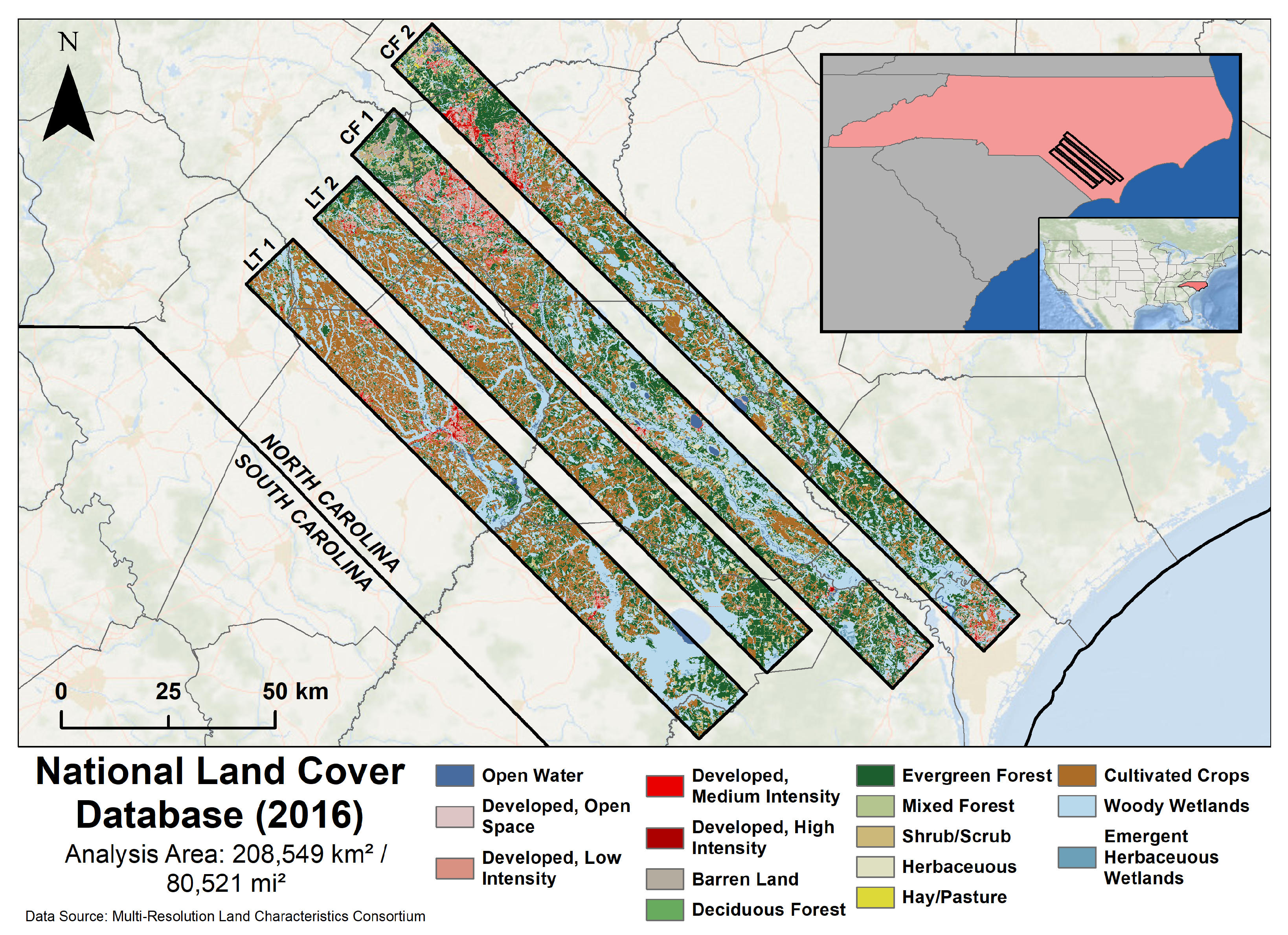
Figure 1. NLCD 2016 land cover types for analysis areas [22]. UAVSAR data swaths are labeled as LT 1, LT 2, CF 1, and CF 2, denoting the Lumber and Cape Fear River basins, respectively.
Remotesensing 13 05098 g001
Figure 2. Visualizations of each distinct scattering mechanism derived from polarized UAVSAR using the Freeman–Durden decomposition (Freeman and Durden 1998).
Remotesensing 13 05098 g002
Figure 3. An overview of the methodology and datasets used to generate flood extent and impact information.
Remotesensing 13 05098 g003
Figure 4. Examples of each land cover type and their respective signatures in the UAVSAR false-color RGB and Planet true color imagery. Histogram distributions of each Freeman–Durden scattering mechanism for the training samples of each class are displayed in the center column.
Remotesensing 13 05098 g004
Figure 5. Histogram distributions of the single, double, and volume scattering intensities of nonforest training pixels for the five days observed between 18 and 23 September 2018.
Remotesensing 13 05098 g005
Figure 6. Histogram distributions of HAND, slope, and water and inundation feature sizes within the LT1 portion of the study area.
Remotesensing 13 05098 g006
Figure 7. A comparison of the RF classifier output and resulting flood estimate following fuzzy logic cleanup and morphological closing. False-color UAVSAR RGB and Planet true-color images are provided for reference.
Remotesensing 13 05098 g007
Figure 8. Calculated importance of each classification feature used for analysis.
Remotesensing 13 05098 g008
Figure 9. Visualizations of the change in estimated flood extent along the Cape Fear River from 18 to 23 September 2018. (a) River flooding in the northwestern portion of Bladen County, NC decreases in extent over the time period. (b) Approximately 60 km to the southeast, portions of the river basin experience an increase in flood extent over the observation period as waters move downstream.
Remotesensing 13 05098 g009
Figure 10. Instances of flood underprediction along the Cape Fear River near Elizabethtown, NC. (A) Misclassifications are evident along the edges of several detected water features. (B) Vegetated areas with emergent plant stems can be misclassified as nonflooded due to enhanced backscatter. (C) Confusion with the urban class is noted in inundated swampy areas with greater spacing between trees.
Remotesensing 13 05098 g010
Figure 11. Visualizations of common sources of flood overprediction. Circled areas denote false detections of open water in visibly dry areas. Arrows indicate false detections of inundated forest along the edges of tree stands. These appear as linear features oriented roughly parallel to the instrument flight path, or from northwest to southeast.
Remotesensing 13 05098 g011
Figure 12. A numerical and visual comparison of flood extent estimations generated from UAVSAR observations and the PNNL RIFT hydrological model for 19 September 2018.
Remotesensing 13 05098 g012
Table 1. Training sample allocation by class proportional area. Total sampling area equal to 0.25% of the total area as recommended by Colditz (2015).
ClassPercent AreaNumber of PixelsTarget Training PixelsActual Training Pixels
Water0.0152,095,82464176421
Dry Forest0.17610,554,31726,40826,400
Inun. Forest0.37715,554,31738,25438,253
Non-Forest0.34813,879,88934,67634,710
Urban0.0837,506,61517,64617,720
Total1.00049,360,182123,401123,504
Table 2. An example of the ground truth point allocation scheme for the LT1 swath on 18 September 2018 following the practices of Olofsson et al. (2014).
ClassWaterDry ForestInundated ForestNon-ForestUrbanTotal
W i (Pixels)761,9578,704,98418,636,79417,186,4114,088,18149,378,327
U i 0.8000.7500.9000.7500.750-
S i 0.7750.7070.8940.7070.707-
Olofsson Method Truth Pixels2771346671854948277521,144
UAVSAR Resolution Adjustment55469314379905554229
Buffered Truth Points55691449956423
Actual Truth Pixels62368814329915654299
Table 3. User and producer accuracies for each RF classification averaged daily and over all fifteen data swaths. Values are percentages.
18 September19 September20 September22 September23 SeptemberEvent Average
Overall Accuracy (OA)86.3687.5789.3786.7188.9087.67
Open Water UA87.8787.5185.0079.2984.8185.65
Open Water PA68.7780.2390.2091.3491.4082.14
Dry Forest UA88.6988.5290.3188.7486.9688.74
Dry Forest PA93.2092.7793.5993.4593.2693.21
Inun. Forest UA93.9094.8295.1496.0695.6094.91
Inun. Forest PA90.6387.8791.7988.7689.6789.78
Non-Forest UA74.4678.9285.2179.1784.3279.74
Non-Forest PA90.1191.8287.9682.2989.4589.01
Urban UA86.5186.1385.6084.6089.0486.31
Urban PA77.6678.7679.0473.9577.4277.70
Table 4. Post-classification user and producer accuracies for open water, inundated forest, and their combined flood extent averaged daily and over the entire observation period. Values are percentages.
18 September19 September20 September22 September23 SeptemberEvent Average
Open Water UA21.2421.2123.5323.1724.8122.42
Open Water PA62.9666.6281.3272.5583.3471.52
Inun. Forest UA73.8872.8969.8370.4967.6271.52
Inun. Forest PA95.1091.9097.1592.8294.8394.31
Floodmap UA47.5647.0546.6846.8346.2146.97
Floodmap PA85.3384.5992.6386.8491.4887.61
Publisher’s Note: MDPI stays neutral with regard to jurisdictional claims in published maps and institutional affiliations.