Upscaling Remote Sensing Inversion Model of Wheat Field Cultivated Land Quality in the Huang-Huai-Hai Agricultural Region, China

Abstract

It is an objective demand for sustainable agricultural development to realize fast and accurate cultivated land quality assessment. In this paper, Tengzhou city (county-scale hilly area: scale A), Shanghe county (county-scale plain area: scale B), and Huang-Huai-Hai region (including large-scale hilly and plain area: scale C and D) were taken as research areas. Through the conversion of evaluation systems, the inversion models at the county-scale were constructed. Then, the image scale conversion was carried out based on the numerical regression method, and the upscaling inversion was realized. The results showed that: (1) the conversion models of evaluation systems (CMES) are Y = 1.021x − 4.989 (CMES_A−B), Y = 0.801x + 16.925 (CMES_A−C), and Y = 0.959x + 3.458 (CMES_C−D); (2) the booting stage is the best inversion phase; (3) the back propagation neural network model based on the combination index group (CI-BPNN) is the best inversion model, with the R² are 0.723 (modeling set) and 0.722 (verification set). CI-BPNN and CI-BPNN-CMES_A−B models are suitable for the hilly and plain areas at the county-scale, and the level area ratio difference is less than 4.87%. Furthermore, (4) the reflectance conversion model of short-wave infrared 2 is cubic, and the rest are quadratic. CI-BPNN-CMES_A−C and CI-BPNN-CMES_A−C-CMES_C−D models realized upscaling inversion in the hilly and plain areas, with the maximum level area ratio difference being 1.60%. Additionally, (5) the wheat field quality has improved steadily since 2001 in the Huang-Huai-Hai region. This study proposes an upscaling inversion method of wheat field quality, which provides a scientific basis for cultivated land management and agricultural production in large areas.

1. Introduction

Cultivated land is the essence of land and the material basis for human survival and development. Cultivated land quality (CLQ) reflects the productive capacity of cultivated land, which is essential for food security, the maintenance of agricultural ecosystem functions, and biodiversity [1,2]. For China, being a large population country in the world, the protection and utilization of cultivated land resources are essential, and the maintenance and improvement of CLQ are facing more significant challenges [3]. Huang-Huai-Hai agricultural region is the main wheat production base in China. Due to natural and human factors, there are many problems in cultivated land quantity and quality [4,5]. Therefore, scientific assessment and rapid monitoring of wheat field CLQ have become an urgent need for agricultural production and sustainable development in the Huang-Huai-Hai region.

Although CLQ is comprehensive, complex, and difficult to quantify, it is a mainstream method to construct an evaluation system based on observable indicators using geographic information systems (GIS) technology [6,7,8]. However, it is difficult to achieve rapid evaluation and dynamic update of CLQ for large regions due to the heavy workload and protracted cycle of field investigation and laboratory detection [9]. With its advantages of comprehensive coverage, low cost, strong spatial and temporal continuity, accuracy, and reliability, satellite remote sensing (RS) has become an indispensable tool in acquiring and monitoring cultivated land information [10,11]. Therefore, how to select remote sensing indicators for evaluation, estimate CLQ quickly and efficiently, and analyze its spatio-temporal variation has become a focus of current research.

In recent years, scholars have explored the comprehensive utilization of land evaluation and remote sensing technology. Multi-source satellite data was widely used in CLQ evaluation. High resolution satellite data was used in CLQ analysis at small and medium scales. For example, Wu et al. [12], Fathizad et al. [13], and Binte Mostafiz et al. [14] adopted different methods to realize CLQ evaluation based on Landsat series data (30 m) at a small scale. Moreover, Fang et al. [15], Xia et al. [16], and Zolekar et al. [17] realized land evaluation analysis based on SPOT (10 m), GF-1 (8 m), and IRS (5.8 m) data at a small scale. However, the CLQ inversion in a large region is difficult due to its low temporal resolution and limited coverage. Therefore, low resolution satellite data has been widely used in CLQ analysis at a large scale. Xu et al. [18], Sciortino et al. [19], and Yu et al. [20] used low-resolution MODIS series data products (250 m/500 m/1 km) to realize CLQ evaluation at a local and national scale, respectively, but the spectral confusion is serious, and the model accuracy is limited. Generally speaking, the current research mainly focused on a single scale, and there were few remote sensing studies on CLQ at different scales. At the same time, the CLQ varies significantly at different scales due to the heterogeneity of CLQ, the non-linearity of remote sensing indicators and response functions, and the difference in image resolution [21]. The inversion model at a small scale is difficult to directly apply to other scales due to the scale variation of CLQ and remote sensing images [22,23]. Therefore, how to better screen remote sensing indicators of CLQ, make full use of the complementarity of different resolution images, carry out scale conversion of inversion model, and realize high-precision joint inversion of large-scale CLQ remains to be further explored.

Therefore, this paper took the Huang-Huai-Hai agricultural region as the research area, and constructed the CLQ model based on OLI (operational land imager) data in typical counties (Tengzhou city and Shanghe county). Additionally, MODIS (moderate-resolution imaging spectroradiometer) images were then used to carry out the upscaling conversion to realize the inversion and dynamic variation analysis of wheat field quality. This paper explores the remote sensing model of wheat field quality and provides technical support for cultivated land management and agricultural production in large areas.

2. Materials and Methods

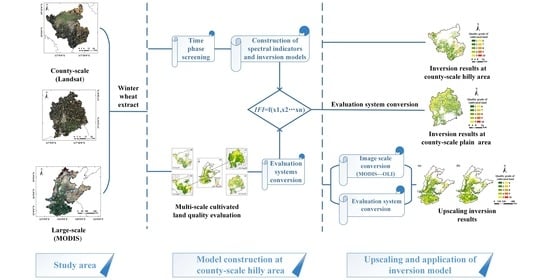
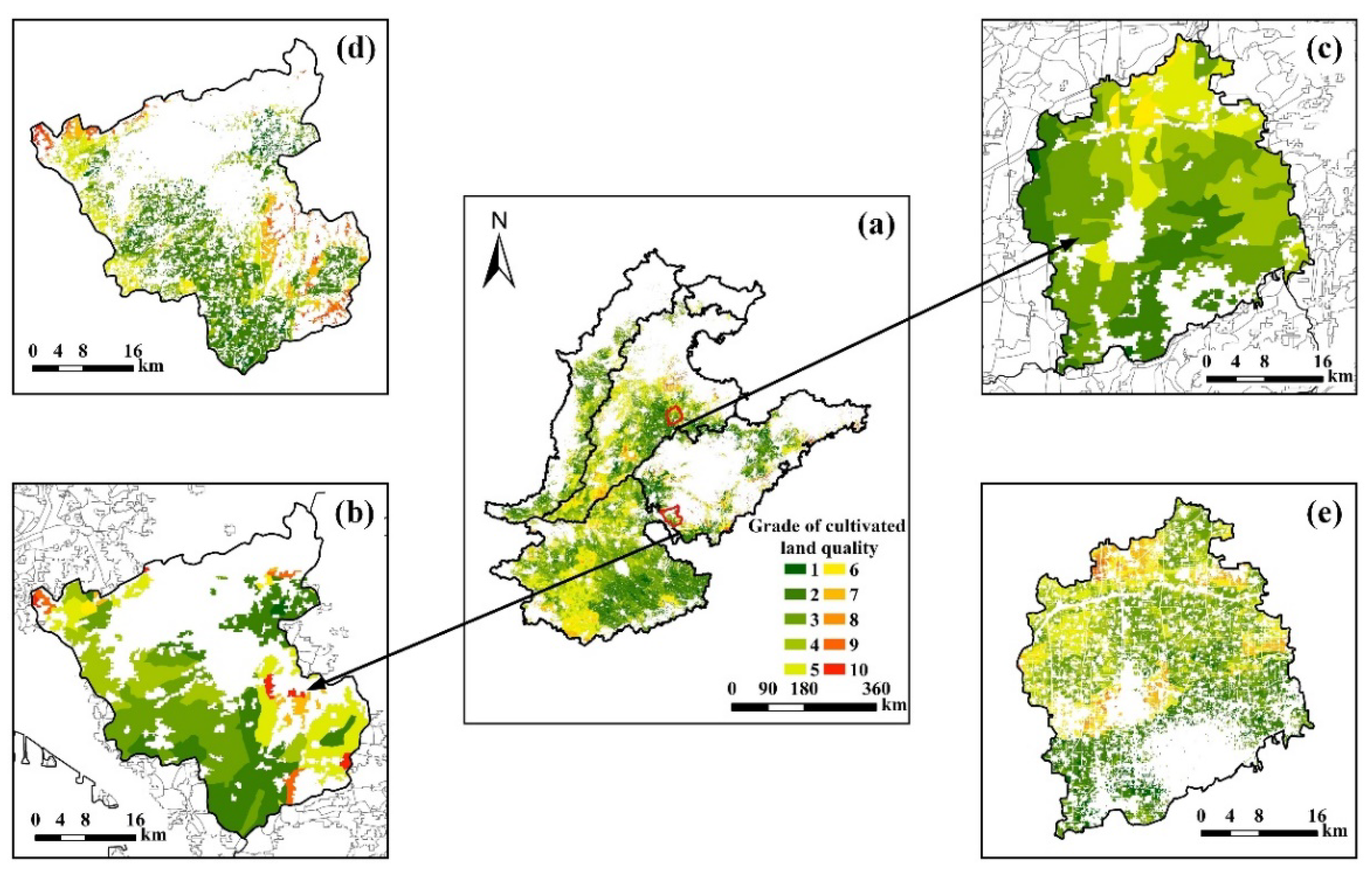
2.1. Study Area

In this study, the Huang-Huai-Hai region was taken as a large-scale research area, Tengzhou city (county-scale hilly area) was taken as the core area for model construction, and Shanghe county (county-scale plain area) was taken as the area for model verification.

The Huang-Huai-Hai agricultural region is located in the east of mainland China (32°23′~41°03′ N, 112°01′~122°42′ E), and includes two plain-type secondary zones (large-scale hilly area) and two hilly-type secondary zones (large-scale plain area), covering 441 counties (cities and districts) [4]. The Huang-Huai-Hai Plain belongs to the warm continental monsoon climate, which is rich in heat resources. The area is low and flat, with plains, low mountains, hills, and other geomorphic types. The cultivated land use types are mainly irrigated land, upland land, paddy field, etc., and there are 19 soil types, including brown soil, cinnamon soil, ginger black soil, etc. This region is an important grain production base, mainly planting winter wheat, whose sowing area accounts for about 53% of the country, and the yield can reach 61% (2018).

Tengzhou city is located in the Shandong hilly agricultural and forestry zone, which belongs to the warm continental monsoon climate. The soil is mainly brown soil and moisture soil. The cultivated land use is primarily irrigated land, dry land, and irrigated paddy fields. At the same time, winter wheat is widely distributed, and the growth difference is noticeable, which is an ideal area for CLQ inversion. This area is similar to the Huang-Huai-Hai region in climate, topography, soil, and cultivated land utilization, and has typical representativeness. Shanghe county is located in the low-lying plain agricultural zone in Hebei, Shandong, and Henan, with low terrain, a high agricultural development level, and extensive winter wheat planting. Therefore, it has a good representation of the plain area and is an ideal model area for regional linkage verification (Figure 1).

2.2. Data Source and Preprocessing

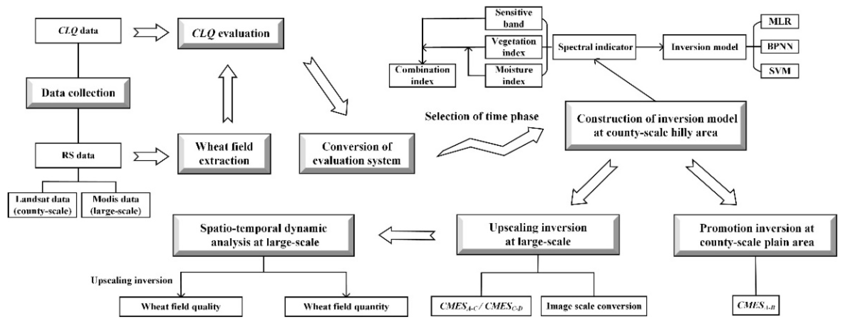
The CLQ evaluation data were mainly derived from the cultivated land quality grade evaluation project of the Huang-Huai-Hai region in 2018, and the cultivated land fertility evaluation, soil testing, and formula fertilization project of Tengzhou city and Shanghe county in 2018. The data content includes sampling sites, thematic maps (such as topographic maps, soil maps, and administrative zoning maps), and relevant statistical data. The wheat field area was obtained through the statistical yearbook and the national economy and social development bulletin.

The required remote sensing images include Landsat OLI and MODIS data. Four Landsat-OLI images at the greening stage (16 March 2018) and the booting stage (17 April 2018) were obtained for wheat field extraction and inversion at the county-scale from the United States Geological Survey (http://glovis.usgs.gov (accessed on 15 August 2021)). As for the Huang-Huai-Hai region, the MODIS series data were derived from LAADS DAAC (https://ladsweb.modaps.eosdis.nasa.gov (accessed on 15 August 2021)). Among them, MOD13Q1 was selected for wheat field extraction from 29 September 2017 to 26 June 2018; and MOD09A1 was selected for upscaling inversion at the booting stage (15 April 2018) of winter wheat. In addition, the MOD13Q1 (29 September 2000 to 26 June 2001, 30 September 2009 to 26 June 2010) and MOD09A1 (15 April 2001, 15 April 2010) data were selected for multi-temporal wheat field extraction and quality inversion.

The IDW method was used to interpolate nutrients, and the statistical data was summarized and sorted by Excel. For Landsat data, ENVI software was used for radiometric calibration, atmospheric correction, geometric precision correction, and image cropping. For MODIS data, the MRT tool was used for image mosaic, band screening, and projection conversion. ArcGIS was used for cropping, ENVI was used for band synthesis, and the Hants method was used for smoothing processing to obtain long time-series MODIS data.

2.3. Methods

Based on realizing the CLQ evaluation and system conversion, this study built an inversion model at county-scale, and realized CLQ inversion and dynamic monitoring in the Huang-Huai-Hai region through upscaling conversion of images and evaluation systems. The technology roadmap is shown in Figure 2, which is mainly divided into the following steps:

Firstly, the primary research data were collected and preprocessed.

Secondly, CLQ evaluation and system conversion. Taking the wheat field extracted from RS as the data source, this chapter evaluated the CLQ and realized the linkage between multiple systems through the linear model.

Thirdly, model construction at county-scale. After determining the best inversion phase, the estimation model was obtained by constructing spectral indicators and inversion models at the hilly area. The inversion was realized by the conversion of evaluation systems at the plain area, and then the accuracy was verified.

Fourthly, upscaling inversion at large-scale. In this chapter, the “numerical regression method” was used for upscaling conversion of images. On this basis, the upscaling inversion was realized through the scale conversion of evaluation systems, and the inversion accuracy was analyzed.

Fifthly, CLQ dynamic analysis. The temporal and spatial dynamics of cultivated land quantity and quality were analyzed from 2001 to 2018.

2.3.1. CLQ Evaluation Based on GIS and Evaluation Systems Conversion

(1)

Wheat Field Information Extraction

Firstly, we set up sample points (training points: verification points = 2:1) according to the characteristics of the study area, spectral, and soil and land use distribution. Secondly, the wheat field information was extracted by the supervised classification method based on OLI images in the greening period at the county-scale and by the random forest classification method (through ENMAP Box software [24]) based on MODIS-NDVI data of the whole growing period at large-scale [25]. Thirdly, the area classification accuracy (ACC_area) was used to reflect the area difference between remote sensing extraction and the statistical yearbook, and the verification point classification accuracy (ACC_point) was calculated by the proportion of verification points that were correctly classified.

(2)

CLQ Evaluation Based on GIS

In this study, the CLQ was evaluated at county-scale (plain area and hilly area) and large-scale (plain area and hilly area) according to the cultivated land quality grade (GB/T 33469-2016) [26]. First of all, the administrative zoning map, soil map, land use status map, and wheat field map were superimposed to realize the division of evaluation units. Secondly, the Delphi method and system clustering method were used to select evaluation factors. Thirdly, the Analytic hierarchy process (AHP) method was used to determine the indicator weight ($C_i$), and the Delphi method and fuzzy statistics method were used to determine the membership degree ($F_i$). Finally, the integrated fertility index (IFI) was calculated, and CLQ grade was divided by the equal space method. The specific formula is as follows:

$$IFI={\displaystyle \sum }_{i=1}^n\left(C_i\times F_i\right);$$

(1)

where $C_i$ represents the combined weight of the $i$th indicator, and $F_i$ represents the membership degree of the $i$th indicator.

(3)

Conversion of CLQ Evaluation Systems

This study realized the linkage between different evaluation systems through the conversion model. The idea of model construction was that different evaluation systems were applied to the same data to obtain the IFI in different areas and scales; then, the IFI of corresponding systems was used to construct a linear regression model. The conversion models constructed in this study were as follows:

$$CME{S}_{A-B}:IF{I}_B=F\left(IF{I}_A\right);$$

(2)

$$CME{S}_{A-C}:IF{I}_C=F\left(IF{I}_A\right);$$

(3)

$$CME{S}_{C-D}:IF{I}_D=F\left(IF{I}_C\right);$$

(4)

where CMES_A-B, CMES_A-C, and CMES_C-D represent the conversion models of evaluation systems from the county-scale hilly area to the county-scale plain area, from the county-scale hilly area to the large-scale hilly area, and from the large-scale hilly area to the large-scale plain area. IFI_A, IFI_B, IFI_C, and IFI_D represent the evaluation results at the county-scale hilly area, county-scale plain area, large-scale hilly area, and large-scale plain area, respectively.

2.3.2. Construction of CLQ Inversion Models at County-Scale

(1)

Selection of Optimal Time Phase for CLQ Inversion

The average values of IFI and NDVI were calculated in wheat’s critical growth periods by taking each county as a unit in the Huang-Huai-Hai region; the Pearson correlation coefficient (R) [27] was used to measure the explanatory power of remote sensing data to CLQ in hilly and plain areas, and the optimal time phase was selected.

(2)

Construction of CLQ Inversion Model at County-scale Hilly Area

①

Construction and Screening of Characteristic Spectral Parameters

We constructed a sensitive band group (consisting of OLI bands), vegetation index group (consisting of vegetation index [28]), and moisture index group (consisting of moisture index [29,30,31]). At the same time, the combined index containing multiple spectral bands was obtained by using multiple combination methods for the above spectral index.

Then, the evaluation units corresponding to the training points and the correct classification verification points in Tengzhou city were taken as a modeling set and verification set, respectively. The mean values of spectral indicators and IFI in the evaluation units were taken as independent and dependent variables, respectively. Additionally, the spectral indicators were screened by the correlation coefficient (R) and the variance inflation factor (VIF) [27].

• ②

  Construction and Screening of Inversion Models

Multiple linear regression (MLR), back propagation neural network (BPNN), and support vector machine (SVM) algorithms [32] were used to build the inversion model with the support of SPSS and MATLAB software. Additionally, the inversion model was screened by the determination coefficient (R²) and the root mean square error (RMSE) [33].

(3)

Promotion of CLQ Inversion Model at County-scale Plain Area

Through the CMES_A-B, the inversion model was converted into the plain area (Shanghe county).

(4)

Verification of Inversion Model Accuracy

The inversion accuracy was verified by comparing the spatial distribution and the area differences between evaluation and inversion results.

2.3.3. Upscaling Conversion of CLQ Inversion Model at Large-Scale

(1)

Upscaling Conversion of Remote Sensing Images

The reflectance values of OLI and MODIS images were extracted by the modeling set and validation set, respectively. Then, we took the band reflectance extracted from OLI images ($B_i$) as the dependent variable and the band reflectance extracted from MODIS images ($b_i$) as the independent variable to construct the reflectance conversion model.

(2)

Upscaling Conversion of Evaluation Systems

For the hilly secondary zones, the CMES_A–C was used to realize the upscaling conversion. For the plain secondary zones, the inversion model was first converted to the large-scale hilly region by CMES_A–C and then converted to the large-scale plain region by CMES_C–D. Additionally, the inversion results were obtained by summarizing each secondary zone.

(3)

Verification of Upscaling Inversion Accuracy

The difference of spectral indicators between OLI data (in Tengzhou city) and MODIS data (before and after correction in the Huang-Huai-Hai region) was compared by mathematical statistics analysis (mean, median, standard deviation). Furthermore, the spatial distribution and the area differences were compared and analyzed between evaluation and inversion results.

2.3.4. Spatio-Temporal Dynamic Analysis of Wheat Field Quantity and Quality

On the one hand, the change of wheat field area was analyzed based on the statistical yearbook data and the dynamic attitude model [34]. On the other hand, the CLQ was inverted by using the optimal upscaling model in the three-time phases (2001, 2010, and 2018), and the spatio-temporal variation was analyzed for the past 20 years.

3. Results and Analysis

3.1. The Results of CLQ Evaluation and Conversion Models of Evaluation Systems

3.1.1. The Results of Wheat Field Extracted

After the layout of sample points, 2512, 700, and 725 training points and 1256, 350, and 363 verification points were obtained in the Huang-Huai-Hai region, Tengzhou city, and Shanghe county, respectively. After remote sensing extraction, the supervised classification accuracy is as follows: ACC_area > 93.04%, ACC_point > 91.46%; and the random forest algorithm classification accuracy is as follows: ACC_area > 91.92%, ACC_point > 88.48%, indicating that the extraction results are ideal, which can meet the needs of further research.

3.1.2. The Results of CLQ Evaluation Based on GIS

Figure 3 shows the GIS-based evaluation results at two scales. It can be seen that the wheat field is widely distributed in Tengzhou city, with noticeable grade differences, which is conducive to the model construction. By comparing the evaluation results at different scales in the same area, the CLQ has the same spatial distribution characteristics. However, the CLQ is more fragmented at the county-scale and is covered up by the large-scale. Therefore, regional linkage and upscaling conversion are necessary to achieve large-scale inversion.

3.1.3. Conversion Models of CLQ Evaluation Systems

The conversion models of evaluation systems are Y = 1.021x − 4.989 (CMES_A–B: from county-scale hilly area to county-scale plain area), Y = 0.801x + 16.925 (CMES_A–C: from county-scale hilly area to large-scale hilly area), and Y = 0.959x + 3.458 (CMES_C–D: from large-scale hilly area to large-scale plain area), respectively. The R² > 0.942, and RMSE < 3.559, indicating a significant linear relationship between different evaluation systems. Such models can realize linkage and unification of CLQ in different regions.

3.2. CLQ Inversion Models at County-Scale

3.2.1. The Results of Time Phase Screening

After correlation analysis, it is found that from the regreening stage (late February) to the booting stage (middle and early April), winter wheat begins to proliferate, and its biomass reaches the maximum at the booting stage. Meanwhile, the NDVI index reaches a peak, and its correlation with CLQ also increases; however, from the booting stage to the milking stage (late May), the growth rate gradually slows down, the NDVI index decreases continuously, and the correlation with CLQ also decreases slowly. Therefore, the booting stage is the best time phase for CLQ inversion in plain and hilly areas.

3.2.2. CLQ Inversion Model at the County-Scale Hilly Area

(1)

Characteristic Spectral Parameters

The correlation between various spectral indicators and IFI are shown in

Table 1. Correlation between integrated fertility index (IFI) and spectral indicators.

Spectral Group	Spectral Indicator	R	Spectral Group	Spectral Indicator	R
Sensitive band group	Coastal	−0.316 **	Moisture index group	SWCI	0.613 **
	Blue	−0.424 **		NDMI	0.743 **
	Green	−0.524 **		NDI	0.736 **
	Red	−0.646 **		MSI1	−0.755 **
	NIR	0.706 **		MSI2	−0.738 **
	SWIR1	−0.511 **		GVMI	0.745 **
	SWIR2	−0.615 **		SWIRR	0.608 **
				SIWSI	0.750 **
				WI	0.743 **
Vegetation index group	NDVI	0.729 **	Combination index group	① Green/(NIR-SWIR1)	−0.757 **
	RVI	0.686 **		② Red/(NIR*SWIR1)	−0.738 **
	DVI	0.743 **		③ Red+NIR-SWIR2	−0.761 **
	SAVI	0.761 **		④ DVI+NDMI	0.805 **
	TVI	0.745 **		⑤ NDVI+SWCI	0.736 **
	EVI	0.754 **		⑥ NDVI*MSI2	−0.745 **
	ARVI	0.740 **		⑦ MSI2/GRVI	−0.761 **
	GNDVI	0.718 **		⑧ (NDVI-NDMI)/ (NDVI+NDMI)	−0.750 **
	GRVI	0.683 **

Note: ** represents a significant correlation at the probability level of 0.01, and bold represents the spectral indicators used for model construction after screening.

. In the sensitive band group, NIR is the highest, with R = 0.706. The correlation in the vegetation and moisture index groups is better. Furthermore, the correlation through combined operation is enhanced compared with previous spectral parameters. The final results obtained through R and VIF screening are shown in bold in Table 1.

(2)

CLQ Inversion Models

Table 2. CLQ inversion models based on different variable sets.

Variable Group	Modeling Method	Modeling Set (700)		Validation Set (320)
		R2	RMSE	R2	RMSE
Sensitive band group	MLR	0.579	5.982	0.569	6.297
	BPNN	0.637	5.570	0.618	5.922
	SVM	0.618	5.796	0.616	5.797
Vegetation index group	MLR	0.601	5.825	0.592	6.117
	BPNN	0.658	5.399	0.630	5.852
	SVM	0.654	5.512	0.620	5.571
Moisture index group	MLR	0.601	5.824	0.631	5.829
	BPNN	0.667	5.343	0.624	5.911
	SVM	0.639	5.623	0.632	5.750
Combination index group	MLR	0.673	4.994	0.640	5.041
	BPNN	0.723	4.645	0.722	4.661
	SVM	0.715	4.780	0.717	4.595

shows the inversion models based on different variable sets. From different modeling methods, the prediction accuracy of BPNN and SVM models is significantly better than the MLR model, and BPNN is the best modeling method. From different spectral indicator groups, the combination index model has the best inversion effect. In summary, the modeling set: R² = 0.723, RMSE = 4.645, and the verification set: R² = 0.722, RMSE = 4.661 in the BPNN model based on combination index group (CI-BPNN), with good prediction ability, low error, and strong stability, which is the best inversion model.

3.2.3. CLQ Inversion Model at the County-Scale Plain Area

The CMES_A–B (Y = 1.021x − 4.989) was used to convert the optimal inversion model (CI-BPNN) to obtain the model (CI-BPNN-CMES_A–B) at the county-scale plain area.

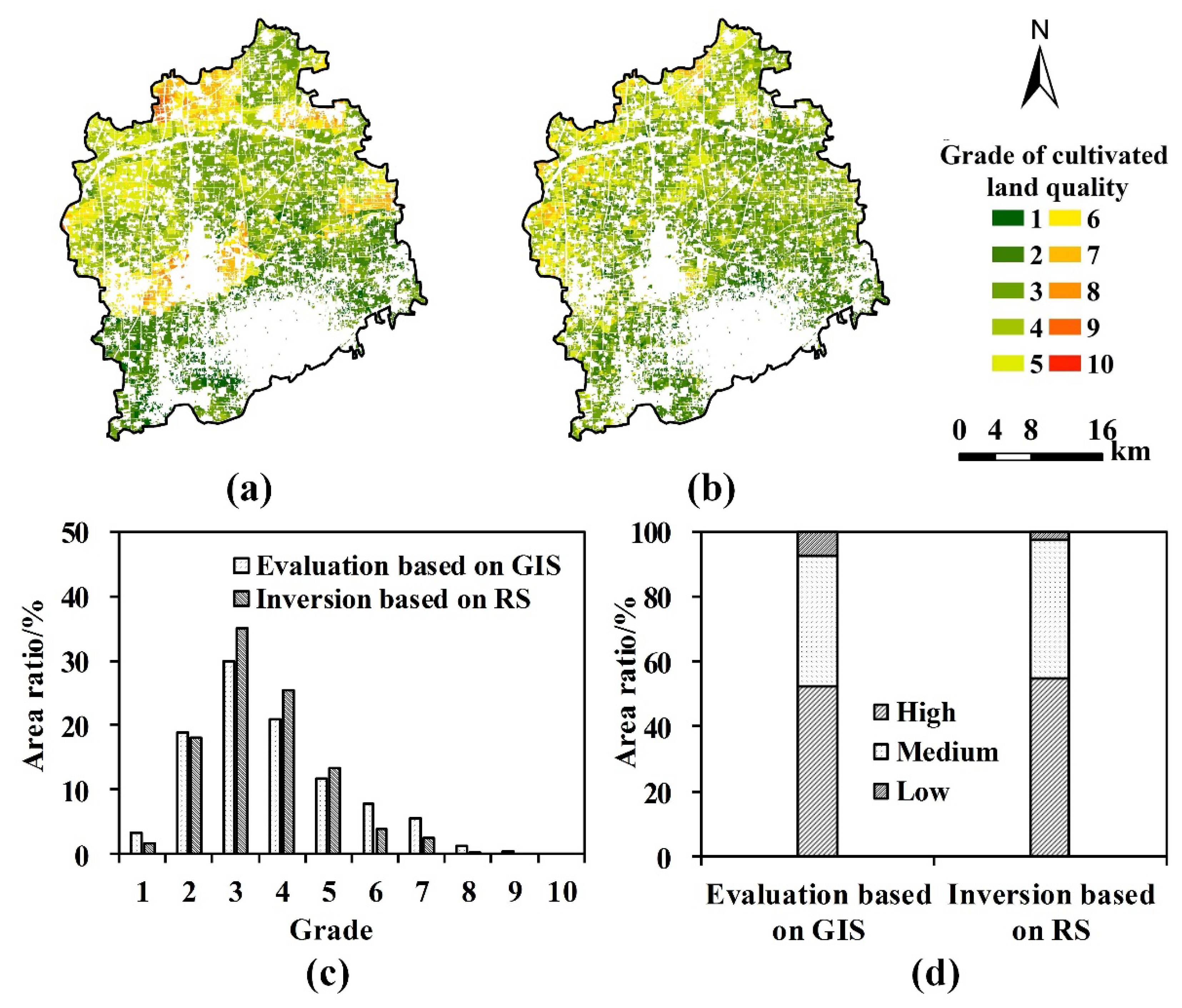
3.2.4. Verification Results of Inversion Accuracy

Figure 4 shows the comparison results of wheat field quality in Tengzhou city (county-scale hilly area) based on GIS evaluation and RS (remote sensing) inversion. The results of Figure 4a,b show that the southwest and northeast are high, and the northwest and southeast are low, with a consistent grade distribution. Furthermore, the area ratio of each grade is similar by comparing Figure 4c,d. When divided into ten grades, the maximum grade area ratio difference is 3.45%; when divided into three levels, the maximum level area ratio difference is 2.91%.

Figure 5 shows the comparison results of wheat field quality in Shanghe county (county-scale plain area) based on GIS evaluation and RS inversion. The results of Figure 5a,b show that the southern is high, and the central and northwest are low, with a consistent grade distribution. Furthermore, the area ratio of each grade is similar by comparing Figure 5c,d. When divided into ten grades, the maximum grade area ratio difference is 5.17%; when divided into three levels, the maximum level area ratio difference is 4.87%.

3.3. The Results of Upscaling Conversion and Model Inversion

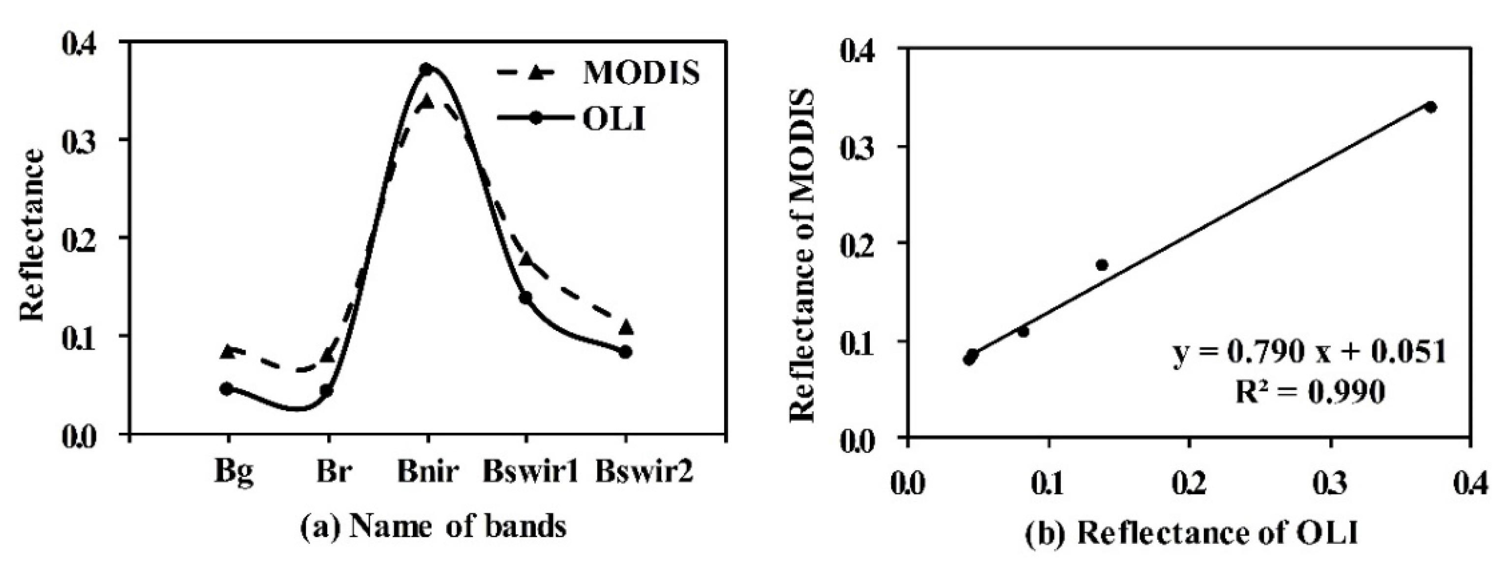
3.3.1. The Results of Images Upscaling Conversion

(1)

Reflectance Comparison between OLI and MODIS Bands

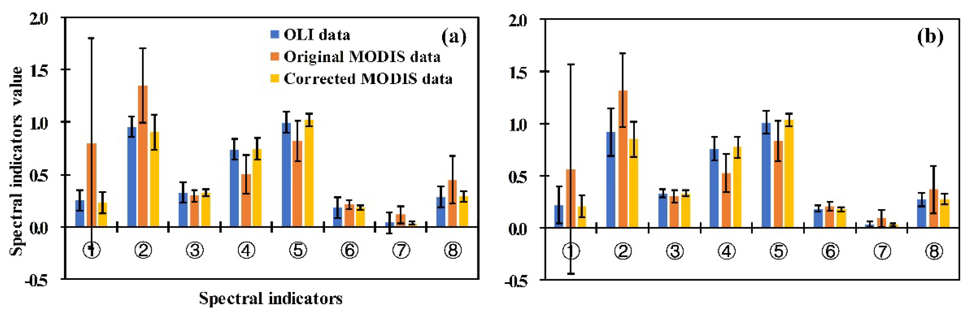
The mean reflectance values of OLI and MODIS images corresponding to the modeling set and validation set were compared (Figure 6a). It was found that OLI’s reflectance is higher than MODIS’s in the near red, while it is the opposite in other bands. Through the correlation analysis from the mean reflectance of each band (Figure 6b), it can be seen that there is a strong correlation, so it is feasible to carry out the upscaling conversion.

(2)

Image Upscaling Conversion Models

The reflectance conversion models are shown in

Table 3. Reflectance conversion models of each band.

Name of Bands	Reflectance Conversion Model	R2	P
Bg	$\mathrm{Y}=0.039-0.105\mathrm{x}+2.163{\mathrm{x}}^2$	0.625	0.000
Br	$\mathrm{Y}=0.047-0.342\mathrm{x}+3.609{\mathrm{x}}^2$	0.636	0.000
Bnir	$\mathrm{Y}=-0.217+2.924\mathrm{x}-3.480{\mathrm{x}}^2$	0.651	0.000
Bswir1	$\mathrm{Y}=0.145-0.343\mathrm{x}+1.658{\mathrm{x}}^2$	0.588	0.000
Bswir2	$\mathrm{Y}=0.071-0.096\mathrm{x}+2.465{\mathrm{x}}^2-6.024{\mathrm{x}}^3$	0.538	0.000

Note: Bg, Br, Bnir, Bswir1, and Bswir2 are bands of green light, red light, near-infrared, short-wave infrared 1, and short-wave infrared 2, respectively.

. Among them, the best model of Bswir2 is cubic, and the rest are quadratic, with R² > 0.5 and p < 0.01.

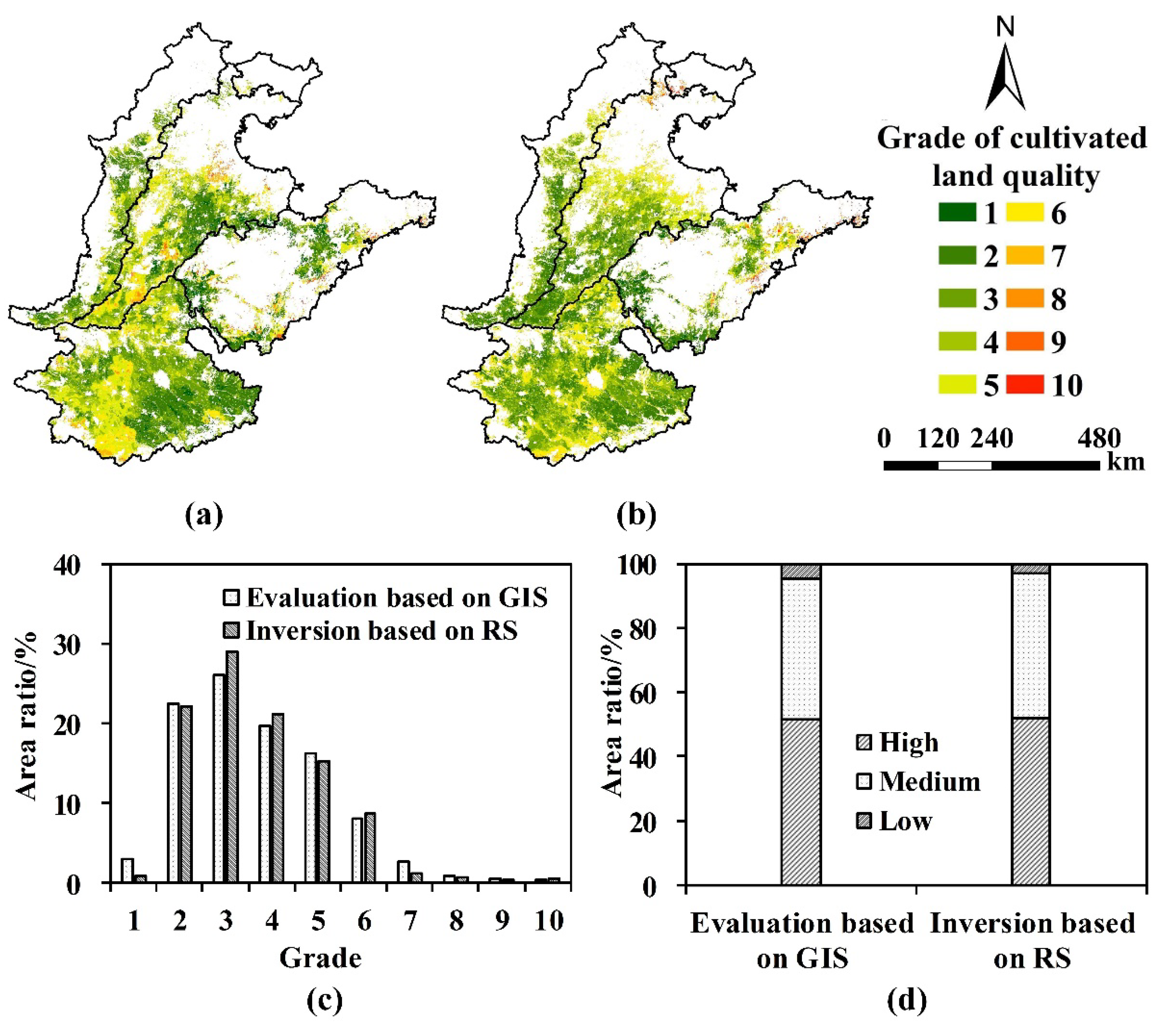
3.3.2. Upscaling Inversion Model at Large-Scale

After realizing the images scale conversion, the CMES were used to convert the upscaling model, and the upscaling scale inversion model in the hilly secondary zones (CI-BPNN-CMES_A–C) and the plain secondary zones (CI-BPNN-CMES_A–C-CMES_C–D) were obtained.

3.3.3. Verification Results of Upscaling Inversion Accuracy

Figure 7 reflects the differences of spectral indicators among image data based on different processing. Compared with OLI data, the difference of mean and median are significant, and the standard deviation difference is noticeable in the original MODIS data. However, after upscaling conversion, the average and median are closer, the standard deviation difference is reduced significantly, and the spectral consistency is better. Therefore, the numerical regression method can enhance the consistency of spectral indicators and realize upscaling inversion.

According to the spatial distribution of upscaling inversion (Figure 8b), high and medium level lands are widely distributed in the Huang-Huai-Hai region. The low-level lands are mainly concentrated in the east of the Shandong hilly agricultural and forestry zone, the south of the Huang-Huai plain agricultural zone, and the north of the low-lying plain agricultural zone in Hebei, Shandong, and Henan, and the Piedmont Plain agricultural zone of Taihang and Yanshan Mountains, consistent with the evaluation results (Figure 8a).

According to the area comparison results (Figure 8c,d), when divided into ten grades, the maximum grade area ratio difference is 2.88%; when divided into three levels, the maximum level area ratio difference is 1.60%. It can be seen that the upscaling inversion model can reflect wheat field quality at a large-scale and has good spatial universality and stability.

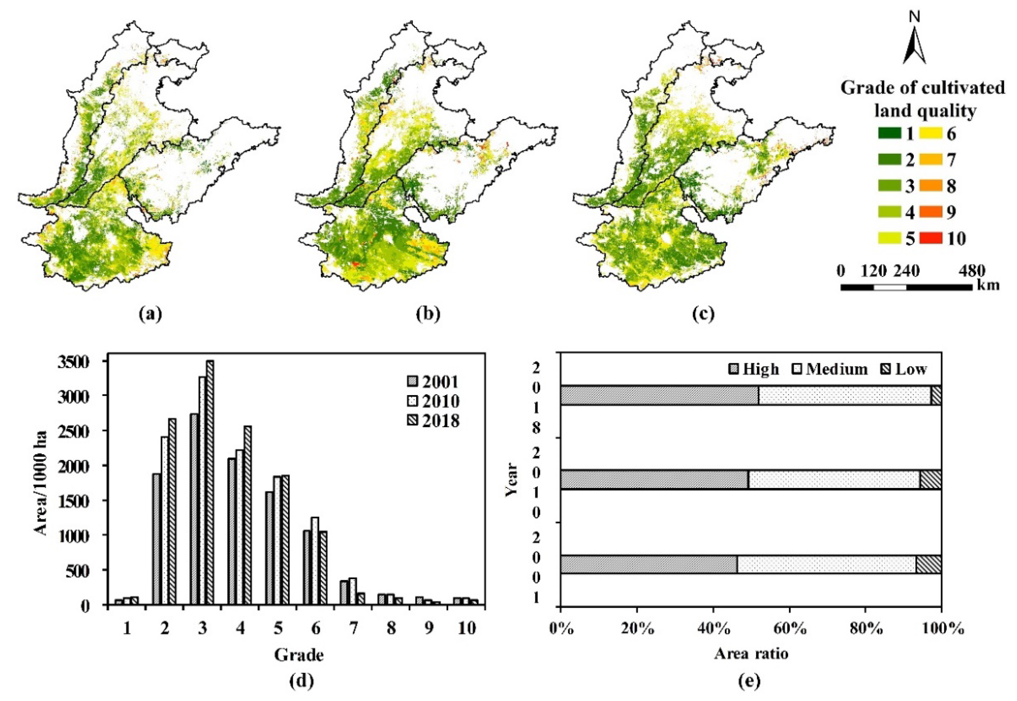
3.4. The Dynamic Analysis Results of Wheat Field Quantity and Quality

3.4.1. Wheat Field Quantity Change

According to the area statistics results in the recent 20 years, the current wheat field area is stable at about 12,000 hectares in the Huang-Huai-Hai region, and the dynamic change rate is steady at –5~5%. The wheat field area had experienced a decrease (2001–2004), an increase (2004–2011), and then finally became stable (2011–now).

3.4.2. Wheat Field Quality Change

Figure 9 reflected the spatio-temporal change of wheat field quality in the Huang-Huai-Hai region. By comparing the inversion results in different phases, it can be seen that the wheat field quality is constantly improving, and the distribution of high-level lands is becoming more and more extensive. According to Figure 9d,e, the high-level lands increased from 46.20% to 51.96%, the middle-level lands were stable, and the low-level lands decreased from 5.65% to 2.87% in the past 20 years.

4. Discussion

Cultivated land is a complex system, and the CLQ shows complex scale variability at different scales [35,36]. In this study, CLQ at different scales in the same region has similar spatial distribution characteristics. The large-scale is more general, highlighting the overall trend, but covers up the variability at the local county-scale. At the same time, the diversity and multiplicity of CLQ were emphasized at the county-scale. CLQ evaluation at different scales should select the appropriate system [37], but different evaluation systems lack comparability. Previous studies had explored the connection between plains and hills [38], but the research on the linkage and conversion between multi-scales was still lacking. This paper has carried out the CLQ link in different regions and scales, with R² > 0.942 and RMSE < 3.559, which provides a reference for relevant research.

Time phase selection is the premise for remote sensing inversion of CLQ. In this paper, the correlation analysis of series MODIS-NDVI data shows that the correlation between NDVI and IFI is the highest at the booting stage, indicating that spectral information has a significant effect on the identification of CLQ. This is similar to the findings of several scholars [39,40]; the leaf area index (LAI), coverage, and biomass of winter wheat in this period reached it’s highest, and NDVI also reached it’s peak, which is a sensitive period for monitoring crop growth and yield, and also becomes the best time phase for CLQ inversion.

The spectral information of wheat growth and soil moisture indirectly represents CLQ [10,41]. Through the analysis of surface spectral characteristics, it is found that the near-infrared band, vegetation index, and moisture index can all reflect the CLQ. Still, the collinearity among indicators is strong, and the model accuracy is difficult to improve. The constructed combination index combines the spectral information of different spectral bands, including visible light, near-infrared and mid-infrared, which overcomes the collinearity problem to some extent and has a stronger correlation with IFI and higher model accuracy. In addition, the land surface temperature is also an important representation of the CLQ. Spectral indicators such as TVDI constructed by vegetation index and land surface temperature information can highlight the surface drought degree. Liu et al. [42] and Airiken et al. [43] have achieved land quality assessment with such indicators, and our study needs to be further strengthened in this respect. From the perspective of modeling methods, machine learning is superior to linear models, the R² of each variable group is improved and the RMSE is reduced, with strong nonlinear fitting and data mining capabilities [44,45]. However, how to further optimize the model and improve the inversion accuracy remains to be studied.

There is a typical linear relationship between the mean reflectance of each band in OLI and MODIS data. Among them, the correlation between near-infrared is the highest, with R² = 0.651. However, the correlation between shortwave infrared 2 is relatively low, with R² = 0.538, which is considered to be due to the significant difference in central wavelength, resulting in the difference in the spectral response of crops [46]. Previous studies have shown that MODIS data’s resolution is low, and the inversion model constructed directly has low accuracy [47,48]. In this study, based on the numerical regression method, the error caused by image scale was “eliminated”, the upscaling application of the inversion model was realized, and the inversion effect was ideal. The image scale conversion based on numerical regression has a simple principle and is easy to implement, but it lacks sufficient extrapolation ability and portability. Gao et al. applied the Bayesian method [49], Pereira et al. applied the geostatistical method [50], and Qi et al. applied the TsHARP method [51] to achieve image scale conversion, respectively. Different methods have their advantages and disadvantages, and how to use other multi-platform remote sensing data to realize the collaborative inversion of CLQ is still worthy of further study.

This paper extracted the wheat field area by the random forest method and inversed the wheat field quality by the upscaling model. The results presented here emphasize the adequate selection of remote sensing indicators for the CLQ evaluation; compared with previous studies [6,7,8,9], it overcomes the disadvantages of time-consuming and tedious traditional survey and evaluation methods, and realizes long-term dynamic monitoring of wheat field information at different scales in the Huang-Huai-Hai region. It will be an effective alternative for the land evaluation of other agricultural territories explored (such as Latin America [52,53], Africa [52] and Asia [54,55]), whose impact would be beneficial when applying techniques such as those developed in our study quickly and efficiently, and when analyzing the spatio-temporal variation of the evaluations. However, the CLQ covered by other crops and its changes need to be further studied.

The techniques developed in our study can allow us to distinguish potentially suitable areas to obtain high levels of productivity and lead to long-term sustainability in these types of important areas. Studies of the CLQ developed in tropical areas [56,57], establish that commercial banana plantations in agricultural areas of the Venezuelan plains were characterized by a considerable reduction in the production and productivity due to a change and deterioration of the land. It was mainly caused by the physical, chemical and biological properties of the soil, these variables being the most determinant of the quality of banana soil in plains. Studies in the subtropical plains have found that soil fertility in a large grain-production area of China has declined [58]. The changes of cropping systems, the differences of fertilization, and the acid rain were the three most important reasons for the changes in recent years. According to the influencing factors of CLQ in different regions, using remote sensing technology to quickly extract sensitive indicators and monitor the dynamic changes of soil fertility will be an important means to prevent soil degradation.

5. Conclusions

This paper constructed the remote sensing inversion model of wheat field quality at the county-scale, and the upscaling inversion was realized at the large-scale by the numerical regression method and regional linkage models. The main conclusions are as follows:

(1)

Conversion models of evaluation systems are Y = 1.021x − 4.989 (CMES_A–B: from county-scale hilly area to county-scale plain area), Y = 0.801x + 16.925 (CMES_A–C: from county-scale hilly area to large-scale hilly area), and Y = 0.959x + 3.458 (CMES_C–D: from large-scale hilly area to large-scale plain area), with R² > 0.942 and RMSE < 3.559, which can realize the CLQ connection in different regions and scales.

(2)

The booting stage is the best time for CLQ inversion. The BPNN model based on the combination index group (CI-BPNN) is the best inversion model, with R² = 0.722 and RMSE = 4.661 (validation precision). The CI-BPNN and CI-BPNN-CMES_A–B models have strong spatial universality and stability at county-scale hilly and plain areas. The maximum level area ratio difference between model inversion and conventional evaluation are 2.91% and 4.87%, respectively.

(3)

For image upscaling conversion, the reflectance conversion model of short-wave infrared 2 is cubic, and the others are quadratic. By converting images and evaluation systems, the upscaling inversion models are CI-BPNN-CMES_A–C (hilly secondary zones) and CI-BPNN-CMES_A–C-CMES_C–D (plain secondary zones), with the maximum level area ratio difference being 1.60%, which has high prediction accuracy and spatial universality.

(4)

Since 2001, the wheat field area has been relatively stable, and the dynamic degree is between −5% and 5%. The wheat field quality has been steadily improved in the Huang-Huai-Hai region, with high-level lands increasing, low-level lands decreasing, and medium-level lands staying relatively stable.

This paper proposes an effective method for upscaling inversion of wheat field quality in the Huang-Huai-Hai region, which provides a scientific basis for obtaining wheat field quality quickly, accurately, and efficiently at different spatio-temporal scales, and guiding agricultural production.

References

1. Mekonnen, M.; Abeje, T.; Addisu, S. Integrated watershed management on soil quality, crop productivity and climate change adaptation, dry highland of Northeast Ethiopia. Agric. Syst. 2021, 186, 102964. [Google Scholar] [CrossRef]
2. Orhan, O. Land suitability determination for citrus cultivation using a GIS-based multi-criteria analysis in Mersin, Turkey. Comput. Electron. Agric. 2021, 190, 106433. [Google Scholar] [CrossRef]
3. Khan, S.; Hanjra, M.A.; Mu, J.X. Water management and crop production for food security in China: A review. Agric. Water Manag. 2009, 96, 349–360. [Google Scholar] [CrossRef]
4. Huang, K.; Liu, Z.; Yang, L.F. Evaluation of winter wheat productivity in Huang-Huai-Hai region by multi-year graded MODIS-NDVI. Trans. Chin. Soc. Agric. Eng. 2014, 30, 153–161. [Google Scholar] [CrossRef]
5. Li, J.D.; Lei, H.M. Tracking the spatio-temporal change of planting area of winter wheat-summer maize cropping system in the North China Plain during 2001–2018. Comput Electron. Agric. 2021, 187, 106222. [Google Scholar] [CrossRef]
6. Yang, Z.F.; Yu, T.; Hou, Q.Y.; Xia, X.Q.; Feng, H.Y.; Huang, C.L.; Wang, L.S.; Lv, Y.Y.; Zhang, M. Geochemical evaluation of land quality in China and its applications. J. Geochem Explor. 2014, 139, 122–135. [Google Scholar] [CrossRef]
7. Raiesi, F.; Kabiri, V. Identification of soil quality indicators for assessing the effect of different tillage practices through a soil quality index in a semi-arid environment. Ecol. Indic. 2016, 71, 198–207. [Google Scholar] [CrossRef]
8. Tashayo, B.; Honarbakhsh, A.; Azma, A.; Akbari, M. Combined fuzzy AHP–GIS for agricultural land suitability modeling for a watershed in southern Iran. Environ. Manag. 2020, 66, 364–376. [Google Scholar] [CrossRef]
9. Zhang, B.; Zhang, Y.; Chen, D.; White, R.E.; Li, Y. A quantitative evaluation system of soil productivity for intensive agriculture in China. Geoderma 2004, 123, 319–331. [Google Scholar] [CrossRef]
10. Weiss, M.; Jacob, F.; Duveiller, G. Remote sensing for agricultural applications: A meta-review. Remote Sens. Environ. 2020, 236, 111402. [Google Scholar] [CrossRef]
11. Eilola, S.; Käyhkö, N.; Fagerholm, N. Lessons learned from participatory land use planning with high-resolution remote sensing images in Tanzania: Practitioners’ and participants’ perspectives. Land Use Policy 2021, 109, 105649. [Google Scholar] [CrossRef]
12. Wu, J.; Li, Z.B.; Li, Y.H.; Zhao, G.X.; Li, C.G. Arable land fertility inversion based on vegetation index from TM image. J. Nat. Resour. 2015, 30, 1035–1046. [Google Scholar] [CrossRef]
13. Fathizad, H.; Ardakani, M.A.H.; Heung, B.; Sodaiezadeh, H.; Rahmani, A.; Fathabadi, A.; Scholten, T.; Taghizadeh-Mehrjardi, R. Spatio-temporal dynamic of soil quality in the central Iranian desert modeled with machine learning and digital soil assessment techniques. Ecol. Indic. 2020, 18, 106736. [Google Scholar] [CrossRef]
14. Binte Mostafiz, R.; Noguchi, R.; Ahamed, T. Agricultural Land Suitability Assessment Using Satellite Remote Sensing-Derived Soil-Vegetation Indices. Landing 2021, 10, 223. [Google Scholar] [CrossRef]
15. Fang, L.N.; Song, J.P. Cultivated land quality assessment based on SPOT multispectral remote sensing image: A case study in Jimo City of Shandong Province. Prog. Geogr. 2008, 27, 71–78. [Google Scholar] [CrossRef]
16. Xia, Z.Q.; Peng, Y.P.; Liu, S.S.; Liu, Z.H.; Wang, G.X.; Zhu, A.X.; Hu, Y.M. The Optimal Image Date Selection for Evaluating Cultivated Land Quality Based on Gaofen-1 Images. Sensors 2019, 19, 4937. [Google Scholar] [CrossRef] [Green Version]
17. Zolekar, R.B.; Bhagat, V.S. Multi-criteria land suitability analysis for agriculture in hilly zone: Remote sensing and GIS approach. Comput. Electron. Agric. 2015, 118, 300–321. [Google Scholar] [CrossRef]
18. Xu, W.Y.; Jin, J.X.; Jin, X.B.; Xiao, Y.Y.; Ren, J.; Liu, J.; Sun, R.; Zhou, Y.K. Analysis of changes and potential characteristics of cultivated land productivity based on MODIS EVI: A case study of Jiangsu Province, China. Remote Sens. 2019, 11, 2041. [Google Scholar] [CrossRef] [Green Version]
19. Sciortino, M.; De Felice, M.; De Cecco, L.; Borfecchia, F. Remote sensing for monitoring and mapping Land Productivity in Italy: A rapid assessment methodology. Catena 2020, 188, 104375. [Google Scholar] [CrossRef]
20. Yu, S.N.; Zhang, X.K.; Zhang, X.L.; Liu, H.J.; Qi, J.G.; Sun, Y.K. Detecting and Assessing Nondominant Farmland Area with Long-Term MODIS Time Series Images. Remote Sens. 2020, 12, 2441. [Google Scholar] [CrossRef]
21. Verburg, P.H.; Chen, Y.Q. Multiscale characterization of land-use patterns in China. Ecosystems 2000, 3, 369–385. [Google Scholar] [CrossRef]
22. Li, X.W.; Wang, Y.T. Prospects on future developments of quantitative remote sensing. Acta Geogr. Sin. 2013, 68, 1163–1169. [Google Scholar]
23. Wu, H.; Tang, B.H.; Li, Z.L. Impact of nonlinearity and discontinuity on the spatial scaling effects of the leaf area index retrieved from remotely sensed data. Int. J. Remote Sens. 2013, 34, 3503–3519. [Google Scholar] [CrossRef]
24. Van der Linden, S.; Rabe, A.; Held, M.; Jakimow, B.; Leitão, P.J.; Okujeni, A.; Schwieder, M.; Suess, S.; Hostert, P. The EnMAP-Box—A toolbox and application programming interface for EnMAP data processing. Remote Sens. 2015, 7, 11249. [Google Scholar] [CrossRef] [Green Version]
25. Skakun, S.; Franch, B.; Vermote, E.; Roger, J.C.; Becker-Reshef, I.; Justice, C.; Kussul, N. Early season large-area winter crop mapping using MODIS NDVI data, growing degree days information and a Gaussian mixture model. Remote Sens. Environ. 2017, 195, 244–258. [Google Scholar] [CrossRef]
26. General Administration of Quality Supervision, Inspection, Quarantine of the (AQSIQ), P.R.C., Standardization Administration of China (SAC). Cultivated Land Quality Grade (GB/T 33469-2016). 2016. Available online: https://www.chinesestandard.net/PDF/BOOK.aspx/GBT33469-2016 (accessed on 1 August 2021).
27. Wang, Z.; Wang, G.; Zhang, G.; Wang, H.; Ren, T. Effects of land use types and environmental factors on spatial distribution of soil total nitrogen in a coalfield on the Loess Plateau, China. Soil Tillage Res. 2021, 211, 105027. [Google Scholar] [CrossRef]
28. Xue, J.R.; Su, B.F. Significant remote sensing vegetation indices: A review of developments and applications. J. Sens. 2017, 2017, 1353691. [Google Scholar] [CrossRef] [Green Version]
29. Zhang, N.; Hong, Y.; Qin, Q.M.; Zhu, L. Evaluation of the visible and shortwave infrared drought index in China. Int. J. Disaster Risk Sci. 2013, 4, 68–76. [Google Scholar] [CrossRef] [Green Version]
30. Zheng, X.M.; Ding, Y.L.; Zhao, K.; Jiang, T.; Li, X.F.; Zhang, S.Y.; Li, Y.Y.; Wu, L.L.; Sun, J.; Ren, J.H.; et al. Estimation of Vegetation Water Content from Landsat 8 OLI Data. Spectrosc. Spectr. Anal. 2014, 34, 3385–3390. [Google Scholar]
31. Wójtowicz, M.; Wójtowicz, A.; Piekarczyk, J. Application of remote sensing methods in agriculture. Commun. Biom. Crop. Sci. 2016, 11, 31–50. [Google Scholar]
32. Chlingaryan, A.; Sukkarieh, S.; Whelan, B. Machine learning approaches for crop yield prediction and nitrogen status estimation in precision agriculture: A review. Comput. Electron. Agric. 2018, 151, 61–69. [Google Scholar] [CrossRef]
33. Sanikhani, H.; Deo, R.C.; Samui, P.; Kisi, O.; Mert, C.; Mirabbasi, R.; Gavili, S.; Yaseen, Z.M. Survey of different data-intelligent modeling strategies for forecasting air temperature using geographic information as model predictors. Comput. Electron. Agric. 2018, 152, 242–260. [Google Scholar] [CrossRef]
34. Xiao, Y.; Zhao, G.X.; Li, T.; Zhou, X.; Li, J.M. Soil salinization of cultivated land in Shandong Province, China—Dynamics during the past 40 years. Land Degrad. Dev. 2019, 30, 426–436. [Google Scholar] [CrossRef]
35. Chen, R.S.; Cai, Y.L. Progress in the study of scale issues in land change science. Geogr. Res. 2010, 29, 1244–1256. [Google Scholar]
36. Verdoodt, A.; Van Ranst, E. Environmental assessment tools for multi-scale land resources information systems: A case study of Rwanda. Agric. Ecosyst Environ. 2006, 114, 170–184. [Google Scholar] [CrossRef]
37. Zhao, Y.F.; Cheng, D.Q.; Chen, J.; Sun, Z.Y.; Zhang, H.N. Problems and analytical logic in building cultivated land productivity evaluation index system. Acta Pedol. Sin. 2015, 52, 1197–1208. [Google Scholar] [CrossRef]
38. Yuan, X.J.; Zhao, G.X.; Zhu, X.X. Linkage of evaluation index system for cultivated land fertility evaluation in plain and hill regions. Trans. Chin. Soc. Agric. Eng. 2008, 24, 65–71. [Google Scholar] [CrossRef]
39. Wardlow, B.D.; Egbert, S.L. Large-area crop mapping using time-series MODIS 250 m NDVI data: An assessment for the US Central Great Plains. Remote Sens Environ. 2008, 112, 1096–1116. [Google Scholar] [CrossRef]
40. Tian, H.R.; Wang, P.X.; Tansey, K.; Zhang, S.Y.; Zhang, J.Q.; Li, H.M. An IPSO-BP neural network for estimating wheat yield using two remotely sensed variables in the Guanzhong Plain, PR China. Comput. Electron. Agric. 2020, 169, 105180. [Google Scholar] [CrossRef]
41. Zhao, C.; Zhou, Y.; Jiang, J.H.; Xiao, P.N.; Wu, H. Spatial characteristics of cultivated land quality accounting for ecological environmental condition: A case study in hilly area of northern Hubei province, China. Sci. Total. Environ. 2021, 774, 145765. [Google Scholar] [CrossRef]
42. Liu, S.S.; Peng, Y.P.; Xia, Z.Q.; Hu, Y.M.; Wang, G.X.; Zhu, A.X.; Liu, Z.H. The GA-BPNN-Based Evaluation of Cultivated Land Quality in the PSR Framework Using Gaofen-1 Satellite Data. Sensors 2019, 19, 5127. [Google Scholar] [CrossRef] [PubMed] [Green Version]
43. Airiken, M.; Zhang, F.; Chan, N.W.; Kung, H.T. Assessment of spatial and temporal ecological environment quality under land use change of urban agglomeration in the North Slope of Tianshan, China. Environ. Sci. Pollut. Res. Int. 2021, 25, 1–18. [Google Scholar] [CrossRef] [PubMed]
44. Babaeian, E.; Paheding, S.; Siddique, N.; Devabhaktuni, V.K.; Tuller, M. Estimation of root zone soil moisture from ground and remotely sensed soil information with multisensor data fusion and automated machine learning. Remote Sens. Environ. 2021, 260, 112434. [Google Scholar] [CrossRef]
45. Danner, M.; Berger, K.; Wocher, M.; Mauser, W.; Hank, T. Efficient RTM-based training of machine learning regression algorithms to quantify biophysical & biochemical traits of agricultural crops. ISPRS Int. J. Geoinf. 2021, 173, 278–296. [Google Scholar] [CrossRef]
46. Zhang, S.M.; Zhao, G.X. A harmonious satellite-unmanned aerial vehicle-ground measurement inversion method for monitoring salinity in coastal saline soil. Remote Sens. 2019, 11, 1700. [Google Scholar] [CrossRef] [Green Version]
47. Jarihani, A.A.; McVicar, T.R.; Van Niel, T.G.; Emelyanova, I.V.; Callow, J.N.; Johansen, K. Blending Landsat and MODIS data to generate multispectral indices: A comparison of “Index-then-Blend” and “Blend-then-Index” approaches. Remote Sens. 2014, 6, 9213. [Google Scholar] [CrossRef] [Green Version]
48. Mondal, P.; McDermid, S.S.; Qadir, A. A reporting framework for Sustainable Development Goal 15: Multi-scale monitoring of forest degradation using MODIS, Landsat and Sentinel data. Remote Sens Environ. 2020, 237, 111592. [Google Scholar] [CrossRef]
49. Gao, S.G.; Zhu, Z.L.; Liu, S.M.; Jin, R.; Yang, G.C.; Tan, L. Estimating the spatial distribution of soil moisture based on Bayesian maximum entropy method with auxiliary data from remote sensing. Int. J. Appl. Earth Obs. Geoinf. 2014, 32, 54–66. [Google Scholar] [CrossRef]
50. Pereira, O.J.R.; Melfi, A.J.; Montes, C.R.; Lucas, Y. Downscaling of ASTER thermal images based on geographically weighted regression kriging. Remote Sens. 2018, 10, 633. [Google Scholar] [CrossRef] [Green Version]
51. Qi, G.H.; Chang, C.Y.; Yang, W.; Gao, P.; Zhao, G.X. Soil salinity inversion in coastal corn planting areas by the satellite-UAV-ground integration approach. Remote Sens. 2021, 13, 3100. [Google Scholar] [CrossRef]
52. Farage, P.K.; Ardö, J.; Olsson, L.; Rienzi, E.A.; Ball, A.S.; Pretty, J.N. The potential for soil carbon sequestration in three tropical dryland farming systems of Africa and Latin America: A modelling approach. Soil Tillage Res. 2007, 94, 457–472. [Google Scholar] [CrossRef]
53. Paredes-Trejo, F.J.; Barbosa, H.A.; Kumar, T.L. Validating CHIRPS-based satellite precipitation estimates in Northeast Brazil. J. Arid. Environ. 2017, 139, 26–40. [Google Scholar] [CrossRef]
54. Shi, Y.Y.; Duan, W.K.; Fleskens, L.; Li, M.; Hao, J.M. Study on evaluation of regional cultivated land quality based on resource-asset-capital attributes and its spatial mechanism. Appl. Geogr. 2020, 125, 102284. [Google Scholar] [CrossRef]
55. Liu, L.M.; Zhou, D.; Chang, X.; Lin, Z.L. A new grading system for evaluating China’s cultivated land quality. Land Degrad. Dev. 2020, 31, 1482–1501. [Google Scholar] [CrossRef]
56. Rondon, T.; Hernandez, R.M.; Guzman, M. Soil organic carbon, physical fractions of the macro-organic matter, and soil stability relationship in lacustrine soils under banana crop. PLoS ONE 2021, 16, e0254121. [Google Scholar] [CrossRef] [PubMed]
57. Olivares, B.O.; Calero, J.; Rey, J.C.; Lobo, D.; Landa, B.B.; Gómez, J.A. Correlation of banana productivity levels and soil morphological properties using regularized optimal scaling regression. Catena 2022, 208, 105718. [Google Scholar] [CrossRef]
58. Chen, S.; Lin, B.W.; Li, Y.Q.; Zhou, S.N. Spatial and temporal changes of soil properties and soil fertility evaluation in a large grain-production area of subtropical plain, China. Geoderma 2020, 357, 113937. [Google Scholar] [CrossRef]
Figure 1. Distribution map of the study area. (a) Huang-Huai-Hai agricultural region; (b) Tengzhou city; (c) Shanghe county. ① and ② represent the plain-type secondary zones (Huang-Huai plain agricultural zone, and low-lying plain agricultural zone in Hebei, Shandong, and Henan), ③ and ④ represent the hilly-type secondary zones (Shandong hilly agricultural and forestry zone, and Piedmont Plain agricultural zone of Taihang and Yanshan Mountains).
Remotesensing 13 05095 g001
Figure 2. Technology roadmap. CLQ: cultivated land quality, RS: remote sensing, RF: random forests, CMESA-B, CMESA-C, and CMESC-D: conversion models of evaluation systems (from county-scale hilly area to county-scale plain area, from county-scale hilly area to large-scale hilly area, and from large-scale hilly area to large-scale plain area).
Remotesensing 13 05095 g002
Figure 3. CLQ evaluation results based on geographic information systems (GIS). (a) Huang-Huai-Hai region; (b) Tengzhou city at large-scale; (c) Shanghe county at large-scale; (d) Tengzhou city at county-scale; (e) Shanghe county at county-scale.
Remotesensing 13 05095 g003
Figure 4. Accuracy analysis of the inversion model at the county-scale hilly area. (a) Spatial distribution map based on GIS evaluation; (b) spatial distribution map based on Remote Sensing (RS) inversion; (c) area ratio comparison between evaluation and inversion at ten grades; (d) area ratio comparison between evaluation and inversion at three levels.
Remotesensing 13 05095 g004
Figure 5. Accuracy analysis of inversion model at the county-scale plain area. (a) Spatial distribution map based on GIS evaluation; (b) spatial distribution map based on RS inversion; (c) area ratio comparison between evaluation and inversion at ten grades; (d) area ratio comparison between evaluation and inversion at three levels.
Remotesensing 13 05095 g005
Figure 6. Comparison of operational land imager (OLI) and operational land imager (MODIS) waveband reflectance. (a) Comparison of the mean reflectance between OLI and MODIS; (b) correlation of the mean reflectance between OLI and MODIS. Bg, Br, Bnir, Bswir1, and Bswir2 are bands of green light, red light, near-infrared, short-wave infrared 1, and short-wave infrared 2, respectively.
Remotesensing 13 05095 g006
Figure 7. Statistics on the mathematical characteristics of spectral indicators from different images: (a) mean; (b) median. ①, ②, ③, ④, ⑤, ⑥, ⑦ and ⑧ are spectral indicators in the combination index group.
Remotesensing 13 05095 g007
Figure 8. Accuracy analysis of inversion model at large scale. (a) Spatial distribution map based on GIS evaluation; (b) spatial distribution map based on RS inversion; (c) area ratio comparison between evaluation and inversion at ten grades; (d) area ratio comparison between evaluation and inversion at three levels.
Remotesensing 13 05095 g008
Figure 9. Dynamic variation analysis of wheat field quality in the Huang-Huai-Hai region. (a) Spatial distribution map in 2001; (b) spatial distribution map in 2010; (c) spatial distribution map in 2018; (d) area ratio change at ten grades; (e) area ratio change at three levels.
Remotesensing 13 05095 g009