Abstract
The availability of remote-sensing multisource data from optical-based satellite sensors has created new opportunities and challenges for forest monitoring in the Amazon Biome. In particular, change-detection analysis has emerged in recent decades to monitor forest-change dynamics, supporting some Brazilian governmental initiatives such as PRODES and DETER projects for biodiversity preservation in threatened areas. In recent years fully convolutional network architectures have witnessed numerous proposals adapted for the change-detection task. This paper comprehensively explores state-of-the-art fully convolutional networks such as U-Net, ResU-Net, SegNet, FC-DenseNet, and two DeepLabv3+ variants on monitoring deforestation in the Brazilian Amazon. The networks’ performance is evaluated experimentally in terms of Precision, Recall, -score, and computational load using satellite images with different spatial and spectral resolution: Landsat-8 and Sentinel-2. We also include the results of an unprecedented auditing process performed by senior specialists to visually evaluate each deforestation polygon derived from the network with the highest accuracy results for both satellites. This assessment allowed estimation of the accuracy of these networks simulating a process “in nature” and faithful to the PRODES methodology. We conclude that the high resolution of Sentinel-2 images improves the segmentation of deforestation polygons both quantitatively (in terms of -score) and qualitatively. Moreover, the study also points to the potential of the operational use of Deep Learning (DL) mapping as products to be consumed in PRODES.
1. Introduction
Deforestation is one of the most serious environmental problems today. The devastation of forests and natural resources compromises the ecological balance and seriously affects the economy and quality of life across the planet.
As the largest tropical forest in the world, the Amazon Rainforest has particular importance. It plays an essential role in carbon balance and climate regulation, provides numerous ecosystem services, and is among the most biodiverse biomes on earth [1]. With about 5 million km, the Brazilian Amazon occupies the largest area of the Amazon Forest, covering about 65% of the total area.
Until 1970, deforestation in the Brazilian Amazon comprised about 98,000 km, while in the last 40 years, the deforested area covered 730,000 km, which corresponds to twice the German territory and comprises nearly 18% of the area formerly covered by vegetation [2,3]. Moreover, the destruction of the Brazilian Amazon rainforest continues at an accelerated rate. Satellite monitoring data published by the Brazilian National Institute for Space Research (INPE) show that the deforestation rate in the Amazon increased by 34% in 2019 compared to the previous year, and the 2020 annual increment of deforestation reached the highest value in the last ten years [4].
The National Institute for Space Research (INPE) has monitored the deforestation rate in the Amazon region since the 1980s through the PRODES (Brazilian Amazon Rainforest Monitoring Program by Satellite (http://www.obt.inpe.br/OBT/assuntos/programas/amazonia/prodes,cyan accessed on 18 July 2021) and the DETER (Real-time Deforestation Detection System (http://www.obt.inpe.br/OBT/assuntos/programas/amazonia/deter, accessed on 18 July 2021) projects [5]). The DETER project is a rapid monitoring system based on medium resolution satellite images, which aims at the early detection of deforestation activities in almost real-time to enable the intervention of security agents before the damage reaches large proportions [6]. The PRODES project, on the other hand, is in charge of accurately mapping deforestation and computing annual deforestation rates. It is based on Landsat-8 images to map the new forest loss that occurred over a year in the Brazilian Amazon biome.
Both the PRODES and DETER protocols involve a great deal of visual interpretation, being consequently a time-consuming process subjected to a significant degree of subjectivity. Although such automatic approaches allow for faster and less subjective analysis, the PRODES and DETER programs still involve considerable human intervention because no entirely automated procedure was able thus far to meet the accuracy requirements.
The literature is plenty of studies aimed at monitoring changes in forest areas based on satellite images [7,8,9]. Many change-detection techniques have been proposed (e.g., [10,11]). Some of the early strategies include techniques based on image algebra [10,12]. Nelson et al. [13] studied image differencing, image rationing, and vegetation index differencing (VZD) for detecting forest canopy alteration. Other change-detection methods proposed thus far rely on machine learning classifiers such as artificial neural networks [14], decision trees [15], fuzzy theory [16], and support vector machines [17].
These change-detection methods present good results for identifying changes in medium- to coarse-resolution imagery but fail when dealing with high-resolution images, tending to produce the salt-and-pepper pattern on the resulting maps [15]. This effect occurs due to high-frequency components and high contrast of the high-resolution images. The image acquisition variation often results in too many changes being detected [15]. Indeed, the method’s main limitation is the difficulty of modeling contextual information as the classes of neighboring pixels are often ignored [18].
In recent years, DL has emerged as the dominant trend in image analysis, performing even better than humans in some complex tasks. Indeed, DL methods have shown great potential in change-detection applications, outperforming traditional machine learning methods (e.g., [19,20,21]). Some approaches in this category involve patch-based classification, including Early Fusion and Siamese CNNs [22,23]. An essential disadvantage of patch classification with CNNs is the redundant operations that imply a high computational cost. The fully convolutional neural networks (FCNs), first proposed in [24], are computationally more efficient by doing pixel-wise instead of patch-based classification. Daudt et al. [25] presented one of the first works using FCNs for change detection. This work adapted patch-based Early Fusion and Siamese Networks into an FCN architecture, having achieved better accuracy and faster computation. Few studies published so far used FCNs for deforestation mapping. De Bem et al. [26] evaluated different machine learning techniques for deforestation mapping in Brazilian biomes based on Landsat-8 images. The comparative study showed a clear advantage of the FCNs over the classic Machine Learning and CNN’s algorithms, both quantitatively and qualitatively.
Most works published thus far pick the class with the highest posterior probability. In deforestation mapping, this means assigning to the class whenever the corresponding posterior probability exceeds 50%, which implies weighting equally false-negatives and false-positives. However, depending on the purpose, false-positives are more detrimental than false-negatives. Consider, for example, a decision whether or not to send a team for inspection and possible infraction notice to a spot suspected of ongoing deforestation activities. The decision to unleash such an action requires confidence in the prediction, for instance, a deforestation probability higher than 50%. In other operational scenarios, the opposite may occur, i.e., false negatives being more harmful than false positives. Therefore, it is worth investigating how the various accuracy metrics behave for different probability thresholds.
This study raises in this scenario and investigates alternative FCN architectures in the Early Fusion configuration for deforestation mapping in the Brazilian Amazon. We further investigate how the different spatial and spectral resolutions of Landsat-8 and Sentinel-2 images, the two currently freely available optical data, may impact the performance of said network designs.
Considering the legend maps are derived from coarse spatial resolution Landsat satellite sensors, we intend to test whether the high resolution of Sentinel-2 images helps to better preserve the spatial structure of the deforestation polygon in comparison with Landsat images.
Specifically, the contributions of this work are three-fold:
- A comparison of six state-of-the-art FCNs, namely U-Net, ResU-Net, SegNet, Fully Convolutional DenseNet, and Xception and MobileNetV2 variants of Deeplabv3+ for mapping deforestation in Amazon rainforest.
- An evaluation of false-positive vs. false-negative behavior for varying confidence levels of deforestation warnings.
- A assessment of said network architectures for detecting deforestation upon Landsat-8 and Sentinel-2 data.
- An unprecedented visual assessment by the PRODES team analysts simulating an audit process of the prediction maps generated by DL networks with the highest performance in both satellites.
The rest of the text is structured as follows: Section 2 presents the FCN architectures investigated in this work. Section 3 describes the study area, the datasets used in our experimental analysis, the experimental setup, the networks’ implementation, and the adopted performance metrics. Next, Section 4 shows the results recorded and, finally, Section 6 summarizes the conclusions derived from the experiments carried out and provides guidance for the continuation of this research.
2. Methods
Fully convolutional networks are the most successful approaches for the semantic segmentation task [24]. Typically, these networks consist of an encoder stage, which reduces the spatial resolution by convolution and pooling operations through consecutive layers, followed by a decoder stage that retrieves the original spatial resolution.
The change-detection algorithm adopted in this work follows the “early fusion” that has been adopted in several related works [23,25,27]. In short, an FC network seeks to identify the pixels where deforestation occurred in the time interval comprised by the acquisition dates of two co-registered images. The input for FC network is the tensor formed by the concatenation of the two images along the spectral dimension.
In this section, we present a short description of the main characteristics of the FCN architectures on which this study is based.
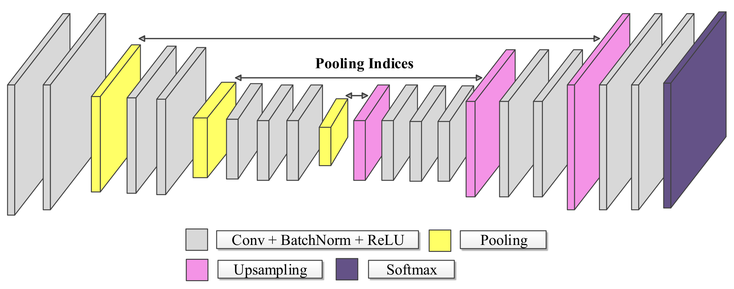
2.1. SegNet
A distinctive feature of this network architecture is the decoding technique, as shown in Figure 1. The encoder stage’s max-pooling operations reduce spatial resolution and computational complexity, causing a loss of spatial information, negatively impacting the outcome, especially at the object borders. SegNet seeks to overcome this downside by storing the maximum pooling indexes in the encoder and using them to recover the fine details’ location in the upsampling operation at the corresponding decoder stage. Compared to U-Net’s skip connections (see next subsection), this strategy allows for a faster training process, as the network does not need to learn weights in the upsampling [28] stage.
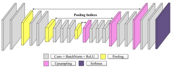
Figure 1.
Basic SegNet Architecture.
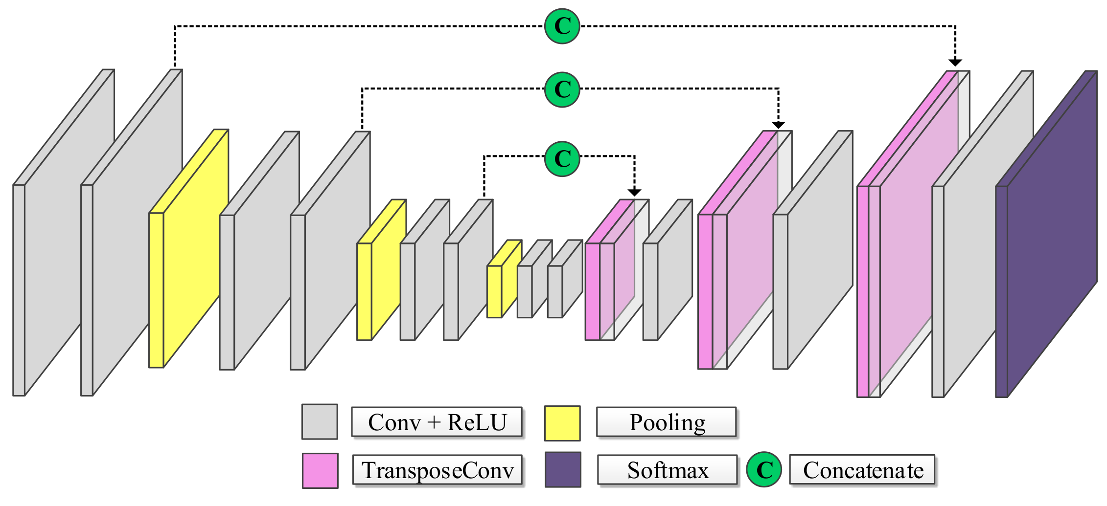
2.2. U-Net
The U-Net is probably the most widely used network architecture for semantic segmentation, see Figure 2. Similar to SegNet, it consists of two sequential stages. First, the so-called encoder successively reduces the spatial resolution as it extracts increasingly coarse features. Then, the decoder continues extracting features at increasingly higher resolutions until it reaches the original resolution and, finally, associates one class to each input pixel position. Characteristic of the U-Net [29] architecture is the skip connections that concatenate features captured in the downsampling path to the features computed by corresponding layers of the upsampling path. In this way, it recovers small details lost through the pooling operations and allows a faster convergence of the model [29].
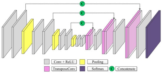
Figure 2.
Basic U-Net Architecture.
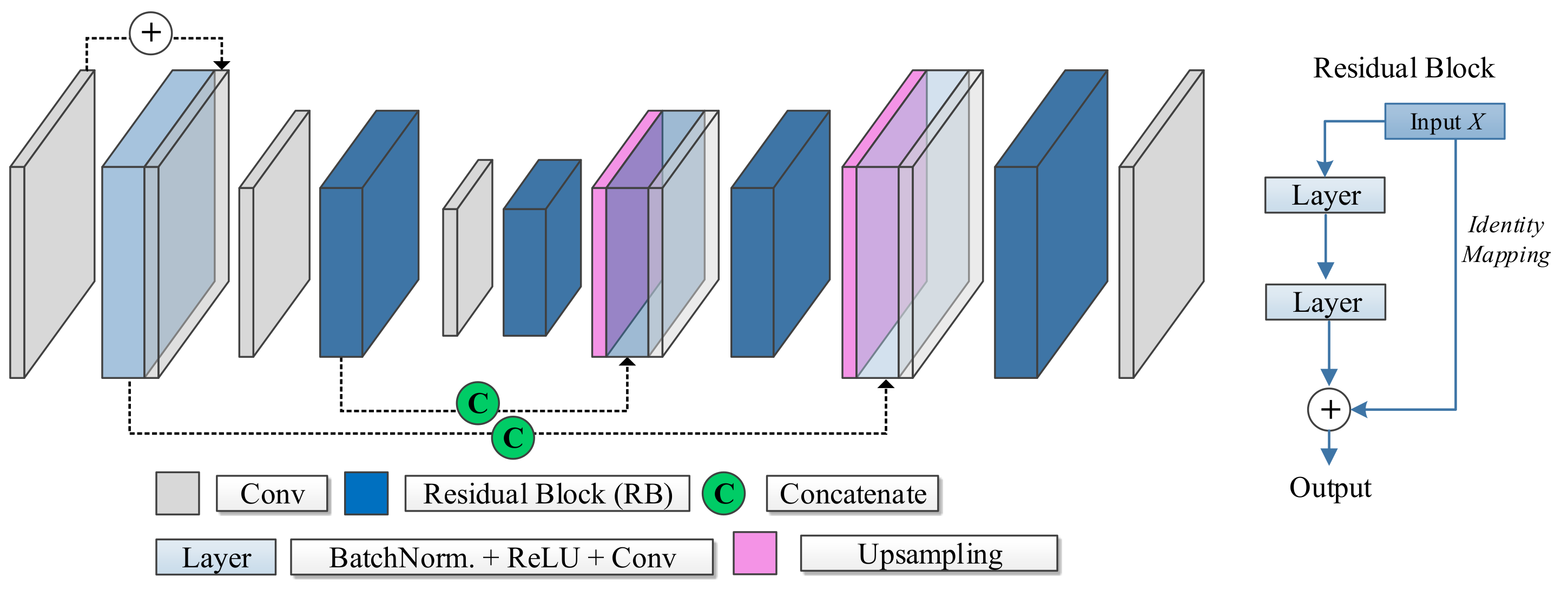
2.3. ResU-Net
ResU-Net [30] is a fully convolutional neural network that takes advantage of both the U-Net architecture and the so-called residual block introduced by the ResNet architecture first conceived for image classification [31]. Residual blocks prevent the vanishing or exploding gradient problem and help this way to create deeper networks. In sum, instead of the input-to-output mapping, a residual block learns the residual to be added to the input to produce the output (see Figure 3 on the right).
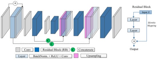
Figure 3.
Basic ResU-Net Architecture, with the residual blocks (RB).
The ResU-Net consists of stacked layers of residual blocks in an encoder-decoder structure. In the encoder stage, a convolution with a stride of 2 downsamples the output of each residual block. The layers within residual blocks are shown in detail in Figure 3. In the decoder stage, the upsampling layers increase the spatial resolution until reaching the original image size. The ResU-Net inherits from the U-Net architecture the skip connections to preserve fine details lost in the encoder stage.
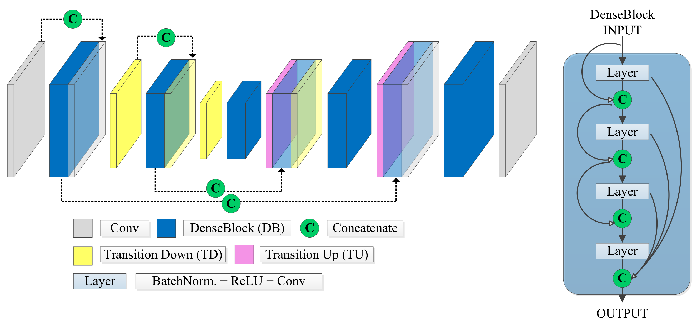
2.4. FC-DenseNet
Jégou et al. [32] extended the Densely Connected Convolutional Network (DenseNet) used for image classification [33] by adding an upsampling path obtaining this way a fully convolutional network for semantic segmentation. The main characteristic of this architecture is its ability to reuse at each layer the preceding layers’ information. The FC-DenseNet concatenates the feature maps computed at each layer with features generated in prior layers forming so-called dense blocks (DB in Figure 4). Therefore, the number of feature maps increases at each new layer. Each block consists of several layers, whereby each layer is composed of batch normalization, a ReLU activation, a 3 × 3 convolution, and dropout.

Figure 4.
Basic FC-DenseNet Architecture from Lobo Torres et al. [34], with the Dense Blocks (DB).
FC-DenseNet uses dense blocks and transition up modules in the upsampling path, which applies transposed convolution to upscale the feature maps up to the original image resolution. The skip connections introduced in the U-Net are also present in FC-DenseNet to recover small details that may go lost along the downsampling path.
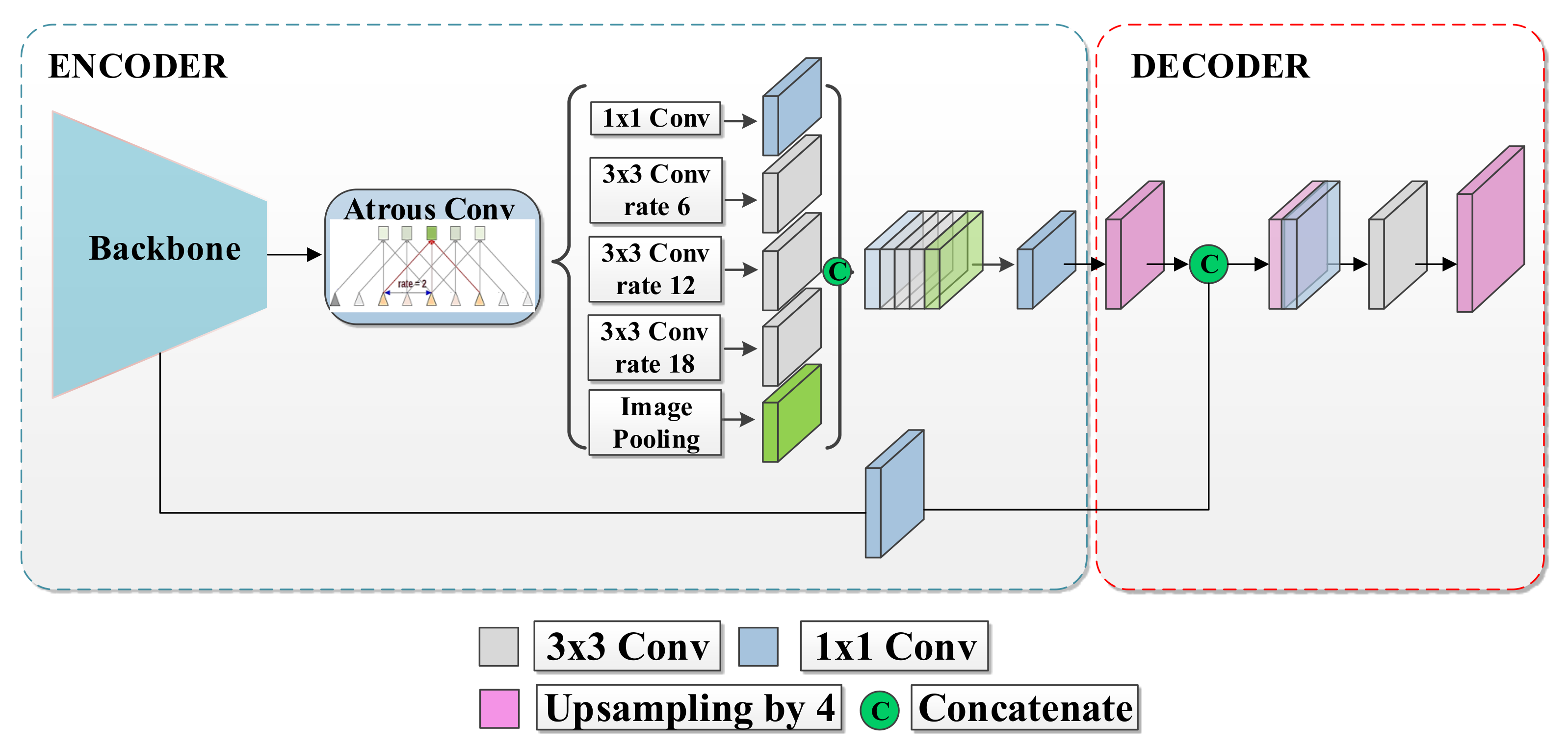
2.5. DeepLabv3+
The DeepLabv3+ model (see Figure 5) has an encoder stage that extracts a compact image representation and a decoder stage that recovers the original image resolution and delivers pixel-wise posterior class probabilities. Compared with previous DeepLab variants, the decoder stage in DeepLabv3+ allows for improved segmentation outcomes along object boundaries [35]. DeepLabv3+ uses the Xception-65 [36] module as a backbone, a deep module based entirely on depthwise separable convolutions [35,36] with different strides. Conceptually, the spatial separable convolution breaks down the convolution into two separate operations: a depthwise and a pointwise convolution [36].
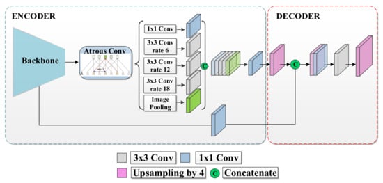
Figure 5.
DeepLabv3+ Architecture.
To increase the field of view without increasing the number of parameters, DeepLab uses the Atrous Spatial Pyramid Pooling in the bottleneck by applying atrous convolution with multiple rates. Atrous convolution, also known as dilated convolution, operates on an input feature map () as follows:
where i is the location in the output feature map , is a convolution filter, and r is the dilation rate that determines the stride in which the input signal is sampled [35].
The basic idea consists of expanding a filter by including zeros between the kernel elements. In this way, we increase the receptive field of the output layers without increasing the number of learnable kernel elements and the computational effort.
Atrous Spatial Pyramid Pooling (ASPP) involves employing atrous convolution with different rates in parallel at the same input as a strategy to extract features at multiple scales. This technique alleviates the loss of the spatial information intrinsic of pooling or convolutions with striding operations [37]. This trick allows for a larger receptive field by increasing the rate value while maintaining the number of parameters.
The decoder is a simple structure that uses the bilinear upsampling to recover the original spatial resolution [35].
2.6. Mobilenetv2
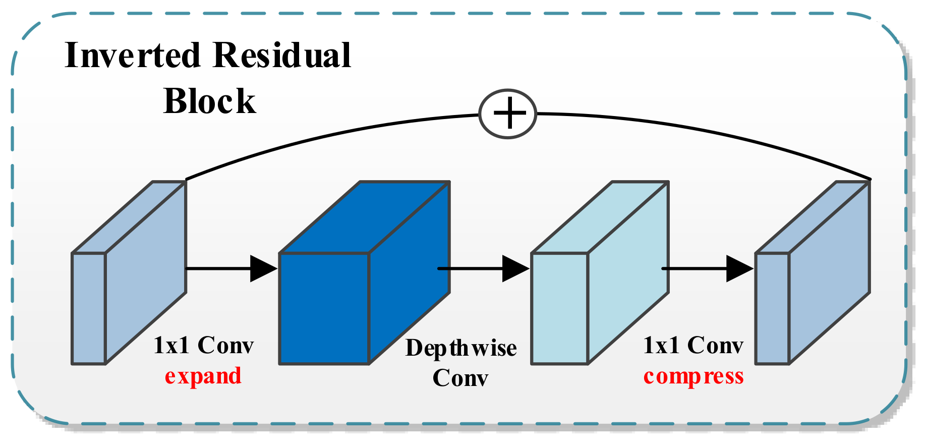
Most of the best-performing FCN architectures require computational resources not available in many mobile devices. This fact moved some researchers to design neural network architectures tailored to mobile and resource-constrained hardware platforms with low accuracy loss. One example is a DeepLabv3+ variant called Mobilenetv2. The architecture’s building blocks are the so-called inverted residual structure [38] (see Figure 6). This module first expands a low-dimensional input to a higher dimension and then applies a lightweight depthwise linear convolution to project back to a low-dimensional representation. Finally, inspired by traditional residual connections, shortcuts speed training and improve accuracy.
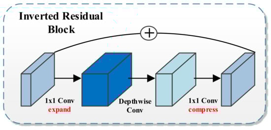
Figure 6.
The inverted Residual Block, the building block of Mobilenetv2.
3. Experimental Analysis
3.1. Study Area
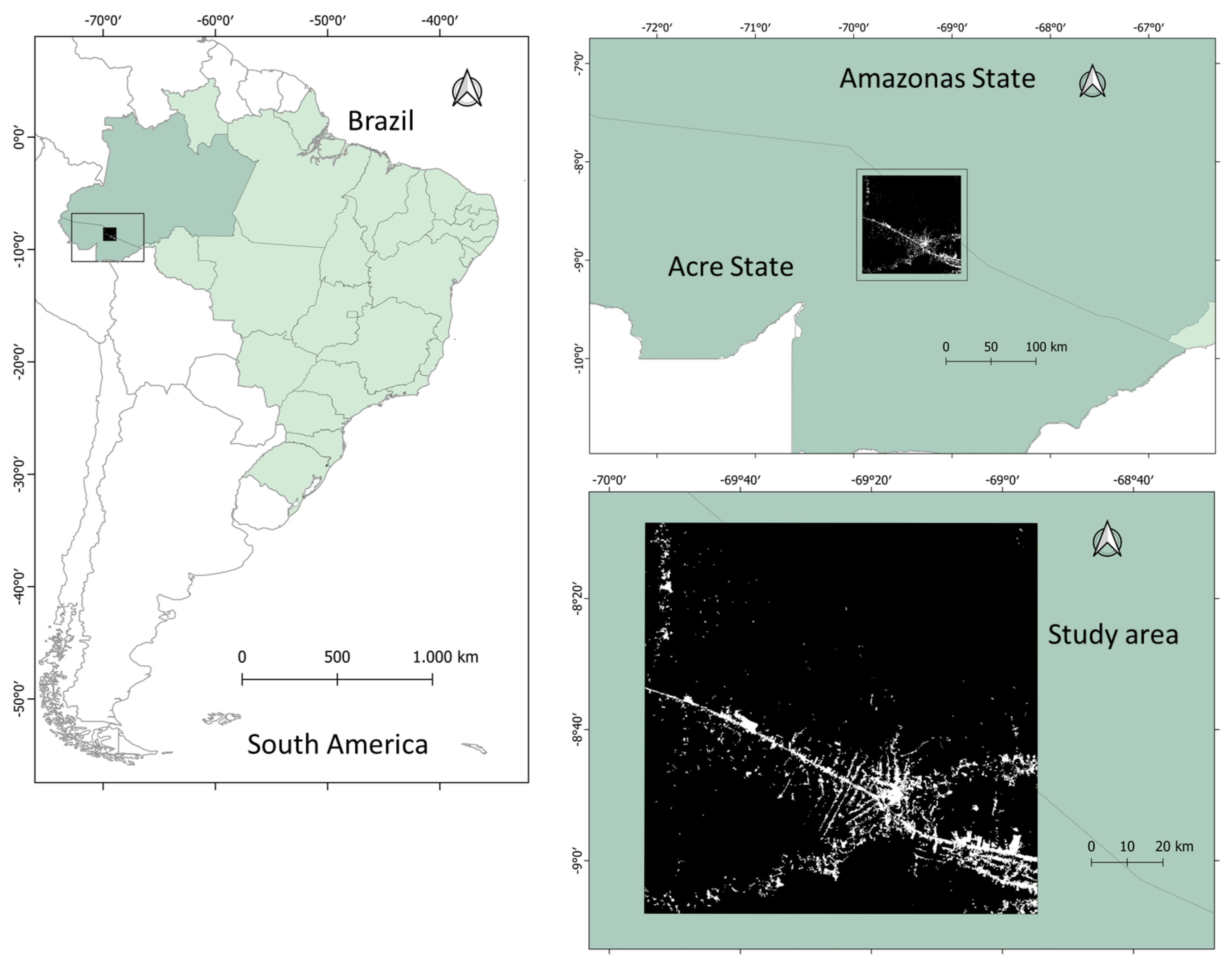
We selected a portion of the Amazon forest in Acre and Amazonas states, Brazil, as a study site (see Figure 7). This area extends over approximately 12,065 km, covering around 0.3% of the total Brazilian Amazon forest. This area intersects with the 003066 Landsat pathrow scene, and its coordinates are 0808 28S–090807S latitude, and 685440W–695429W longitude. The area is characterized by typical Southwest Amazon moist forests and with a lesser presence of flooded forests. Most of the study area has no specific protection status, with less than 5% of the extractivist reserve and indigenous lands on its Southern part. Two aspects strengthen the choice of this area to conduct our experiment: (i) the deforestation patterns diversity, based on landscape metrics and polygon area [39], are represented by multidirectional, geometric regular, linear, and diffused occupation forms and (ii) the deforestation dynamics in the region, characterized by intense occupation along the BR-364 federal road, but also deep inside the forest, and induced by the expansion of agricultural frontier from the Rondonia State to western territories. More than 7% of the study area has already been deforested until 2020.

Figure 7.
Study area at Acre state, Brazil. Image sample correspond to a Sentinel-2 image extension.
3.2. Datasets
We downloaded all datasets used in our experiment from PRODES and DETER websites, which are accessible from TerraBrasilis portal, http://terrabrasilis.dpi.inpe.br/en/home-page/ (accessed on 18 July 2021), where all deforestation reports produced by both programs since they came into operation are available for free.
The input to deep learning models were Landsat-8 Collection 1 Tier 1 (https://developers.google.com/earth-engine/datasets/catalog/LANDSAT_LC08_C01_T1, accessed on 18 July 2021) and Sentinel-2 L1C (https://developers.google.com/earth-engine/datasets/catalog/COPERNICUS_S2, accessed on 18 July 2021) data. These products include radiometric and geometric corrections to generate highly accurate geolocated images without involving secondary preprocessing such as atmospheric corrections. Before feeding the network, we normalized the input data channel-wise to zero mean and unit variance.
The two Landsat-8 images with size 2145 × 3670, and two Sentinel-2 L1C images of size 6435 × 11,010 were acquired between 1 July of 2017 and 21 August of 2018 (see Figure 8a,b). It is not easy to obtain cloudless optical orbital images from the Amazon rainforest for most of the year. That is why PRODES reports refer to deforestation from the dry season of one year to the dry season of the following year. The public PRODES database from which we extracted the data used in this study relies on images acquired around July/August of each year.
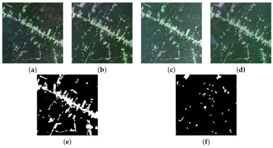
Figure 8.
R-G-B composition of 1 tile of the images at dates 2017 and 2018 (a,b), Landsat-8 images, respectively, (c,d), Sentinel-2 images, respectively (e,f) stand for the Reference 1 (past reference) and Reference 2 (current reference) for both datasets.
We used all Landsat-8 seven bands with 30 m spatial resolution. As for the Sentinel-2 dataset, we used four bands (Blue, Green, Red, and NIR) with 10 m spatial resolution (see Figure 8c,d).
Experienced professionals annotated all images by visual photo-interpretation. They identify change patterns based on three main observable image features: tone, texture, and context. Additionally, they only annotated deforestation polygons with an area greater than 6.25 hectares.
PRODES adopts an incremental mapping methodology for building the deforestation maps. It involves an exclusion mask (see Figure 8e), which covers the areas deforested up to the current date and the residuals (deforestation detected in a given year but referring to the image of the previous year), and a second mask (see Figure 8f), which corresponds to areas deforested in the reference year. The exclusion mask helps the photo-interpreters to delineate polygons of recent deforestation exclusively [2]. Following the PRODES and DETER methodology to calculate accuracy, we disregarded the classification results within a two pixels wide buffer around the prediction and reference polygons, where both are not reliable. To be consistent, we did not consider pixels in these regions either for training or testing.
3.3. Experimental Setup
To model the deforestation dynamics in the study area between two consecutive years, we took pairs of co-registered images acquired in 2017 and 2018, as specified in Section 3.2. We concatenated the co-registered images of each bi-temporal pair along the spectral dimension following the Early Fusion method [23], both for Landsat-8 and Sentinel-2.
We split the images into 15 non-overlapping tiles of 715 × 734 and 2145 × 2202 for Landsat and Sentinel 2 dataset, respectively, and separated the tiles into three groups: 20% for training, 5% for validation, and 75% for testing.
Each tile was further split into equal-sized patches of 128 × 128 pixels yielding a total of 5824 and 17,473 patches from Landsat and Sentinel-2 datasets, respectively.
Both datasets are highly unbalanced. The deforestation class corresponds to less than 1% for both datasets. To alleviate the class imbalance, we applied data augmentation using 90 rotations, horizontal and vertical flip transformations to the patches containing deforestation spots.
To compensate for the class imbalance, we adopted the Weighted Cross-Entropy Loss. The objective was to force FCNs to focus on those weakly represented instances by assigning them a larger weight. Equation (2) represents the Weighted Cross-Entropy Loss for binary classifications,
where N and M stand for the total number of training pixels in rows and columns, respectively, while stand for the weights of the deforestation class. The weights for deforestation class in relation to forested class were empirically set to 5. Moreover, and represent the target and predicted label at pixel .
3.4. Networks’ Implementation
We conducted an exploratory analysis to select the hyperparameter values for each tested network, including several layers, operations per layer, and kernels’ size.The source codes are available at https://github.com/DLoboT/Change_Detection_FCNs (accessed on 18 July 2021). Table 1 presents the network configurations used in our experiments. Table 2 shows the parameters’ setup in each case.

Table 1.
Details of the SegNet, U-Net, and FC-DenseNet architectures used in the experimental analysis of Amazon Deforestation.
Table 2.
Number of parameters of each network for the Deforestation application.
We implemented the networks using the Keras deep learning framework [40] on a hardware platform with the following configuration: Intel(R) Core(TM) i7 processor, 64 GB of RAM, and NVIDIA GeForce RTX 2080Ti GPU. We trained the models from scratch for up to 100 epochs using the Adam optimizer with a learning rate of . Training stopped when the performance measured on the validation set degraded over ten consecutive epochs. In the end, the model that exhibited the best performance on the validation set across all executed epochs kept for the test phase. The batch-size was selected experimentally to 16 for all tested networks.
3.5. Performance Metrics
The accuracy metrics adopted in our analysis were Overall Accuracy, Precision, Recall, and -score, as defined in Equations (3), (4) and (5) respectively.
The overall accuracy is defined as:
where stand for the number of true positives, true negatives, false-positives, and false-negatives samples, respectively. The terms positive and negative refer to deforestation and no-deforestation classes, respectively.
The -score is defined as:
where P and R stand for precision and recall, respectively, and are given by the ratios [41]:
Another metric to report accuracy in our experiments is the Alarm Area (AA) [23]. It gives the proportion of the test area whose deforestation probability delivered by the network exceeds a given threshold, formally:
AA occurs in our analysis in combination with Recall. By varying the deforestation probability threshold, we obtain corresponding pairs of AA and R values that can be plotted in a AA vs. R curve for each tested architecture. AA is related to the amount of human or material resources needed to more closely inspect the areas with deforestation probability above a certain threshold. R, on the other hand, gives the proportion of all deforested areas whose deforestation probability estimated by the automatic method exceeds that threshold. Therefore, the AA vs. R curve provides different tradeoffs between these metrics and subsidizes a decision on which spots to direct the inspection resources in different operational scenarios.
We also report networks’ accuracy in terms of the Average Precision (mAP) defined as the area under the P vs. R curve.
4. Results
4.1. Segmentation Accuracy for Deforestation Detection
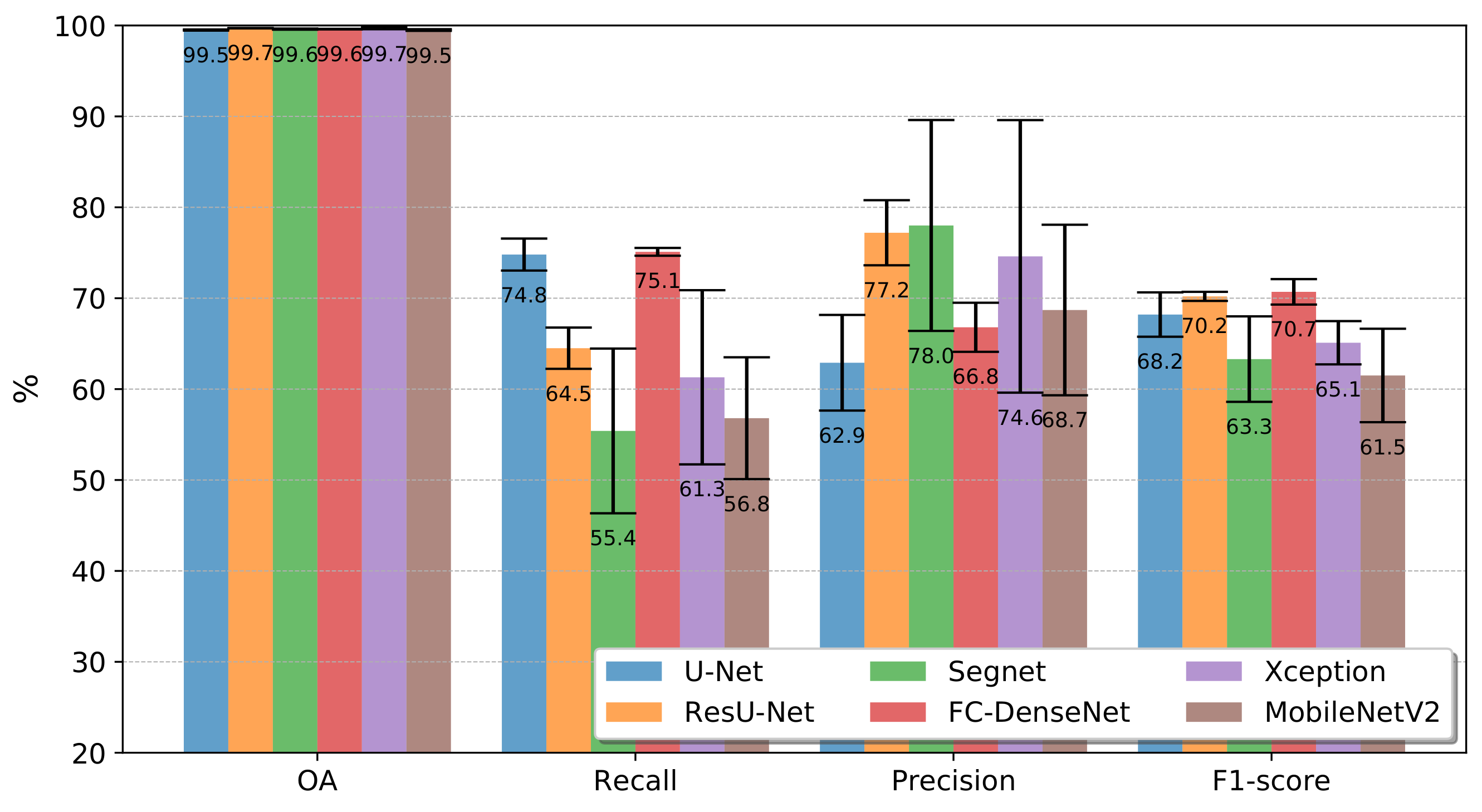
Figure 9 and Figure 10 present the accuracy results obtained by the FCNs in terms of Overall Accuracy, Recall, Precision, and -score for experiments conducted on Landsat-8 and Sentinel-2 data, respectively. The figures summarize the mean values and standard deviations computed after ten runs, each run with the same configuration of training and test samples as described in Section 3.3.
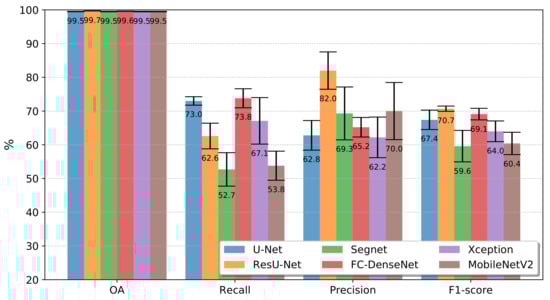
Figure 9.
Mean Overall Accuracy (OA), Recall, Precision, and , over 10 run for the all FCN architectures in the Landsat-8 dataset.
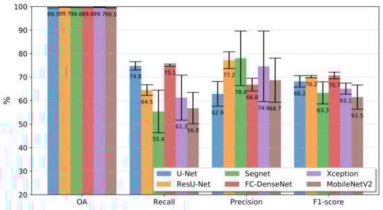
Figure 10.
Mean Overall Accuracy (OA), Recall, Precision, and , over 10 run for the all FCN architectures in the Sentinel-2 dataset.
The first bar group reports the overall accuracies. All networks achieved similar scores, which is little revealing regarding the tested network architectures’ relative performance. Those values correspond approximately to the occurrence of class deforestation in each pair of images. It may raise the question of whether the classifiers merely associated all pixels with the class no-deforestation.
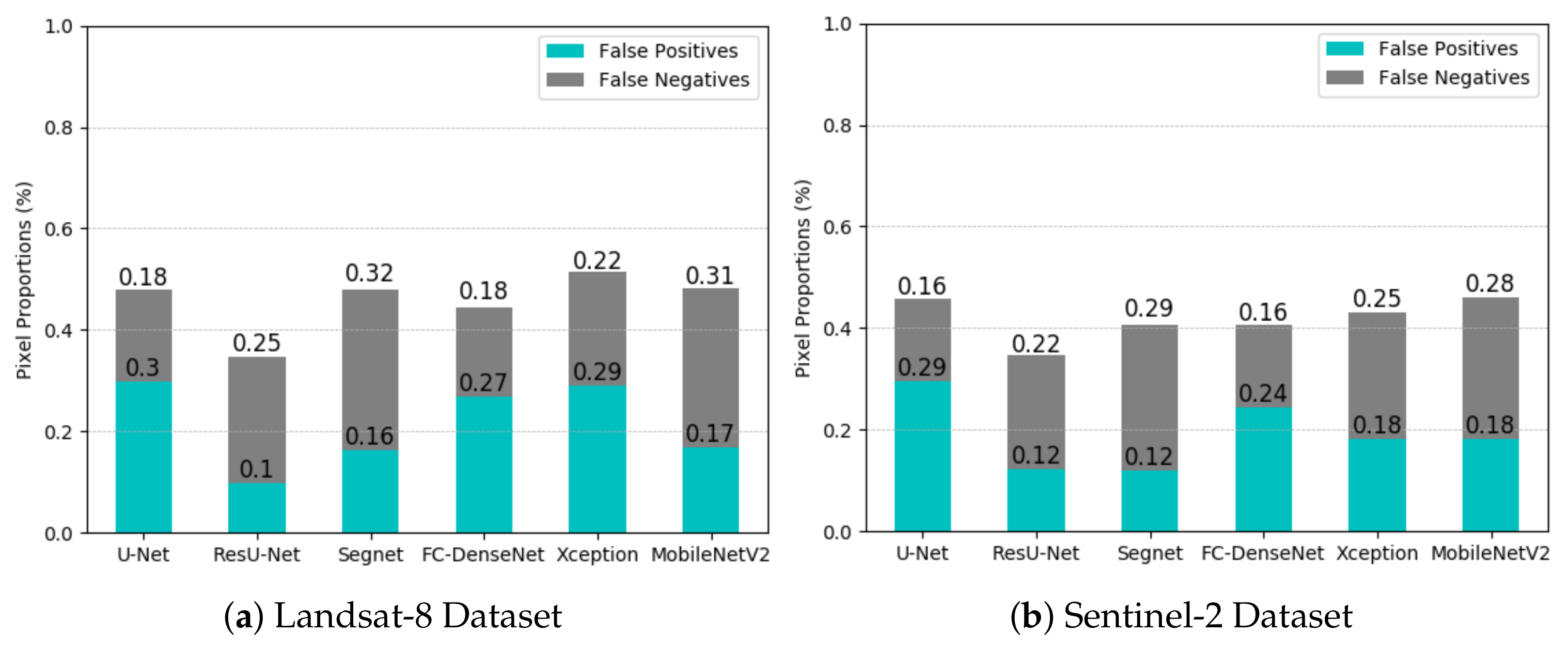
Figure 11a,b clarifies this issue. They show the proportion of false-positives and false-negatives considering the total number of pixels in the test set by each network in the Landsat-8 and the Sentinel-2 datasets, respectively. The analysis of these plots places the ResU-Net as the best-performing network in terms of the total number of classification errors, followed by FC-DenseNet. This ranking remains practically unchanged in the experiments with Landsat-8 and Sentinel-2 data. It is noteworthy a slight reduction of classification errors for all the networks in the Sentinel-2 in comparison with the Landsat-8 dataset.
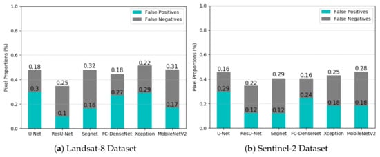
Figure 11.
Proportions of false-positives and false-negatives of each network design.
The second and the third bar groups of Figure 9 and Figure 10 refer to Recall and Precision. According to the Recall metric, FC-DenseNet and U-Net were always the best-performing networks following from Xception in Figure 9, and surpassed for ResU-Net in Figure 10. MobileNetV2 and Segnet always performed among the five and six networks in terms of Recall for both datasets. Unlike Xception, it is also remarkable that the networks achieved the best Recall results for Sentinel-2 data, being MobileNetV2 and Segnet as the most profited networks with a difference considering Landsat-8 of 3% and 2.7%, respectively.
FC-DenseNet and U-net performed among the three lowest Precision results for both datasets, indicating a tendency towards misclassifying deforested areas. In comparison, ResU-Net was always among the top two best-performing networks at a short distance from Segnet in the Sentinel-2 dataset. Please note that Segnet and MobileNetV2 were consistently among the two networks whose results varied the most over the ten runs. Among the datasets, more than the other networks Xception and Segnet showed a clear advantage in the Sentinel-2, with gains of 12.4% and 8.7%, respectively.
The -score in the fourth bar groups of Figure 9 and Figure 10 summarizes in a single value the Recall and Precision for each network and dataset. From the -score perspective, the results obtained for both datasets lead to the same conclusion: ResU-Net and FC Densenet achieving the highest score followed by U-Net and Xception, and Segnet and MobileNetV2 as the worst-performing networks. Additionally, in terms of variation over the ten runs, Segnet and MobileNetV2 presented the worst behavior.
The inferior performance of the Segnet could lie in the manner in which recovered the spatial resolution in the decoder stage. Specifically, the upsample maps in Segnet employ interpolation, while ResU-net, FC-DenseNet, and U-net used transposed convolution. Furthermore, the essential spatial information is better preserved by the skip connections of the ResU-net, FC-DenseNet, and U-net than the pooling indices in the Segnet.
On the other hand, the DeepLabv3+ variants can encode greater contextual information; nevertheless, along with Segnet it ranked in the last tree positions in the experiments with both datasets. It would seem that the use of more contextual information did not impact these results given the low-scale variability of the deforestation polygons in our application.
As stated before, the Xception variant overcame the MobileNetv2 in all cases. Since MobileNetv2 is a lightweight version of Xception, we argue that the latter produced better results due to its greater complexity. This is attested by all the quantitative results shown in Figure 9 and Figure 10.
Concerning the difference of both datasets, except ResU-net, all the networks performed better in Sentinel-2 in terms of -score. Again, we also noticed that MobileNetv2 and Segnet benefited more than all other architectures.
For the results reported in Figure 9, Figure 10 and Figure 11, we assigned to the class deforestation all pixels which probability delivered by the corresponding network exceeded a threshold equal to 50%.
We applied McNemar’s test to each pair of network models evaluated in this work, taking as the null hypothesis that the tested models presented similar performance. Each model was represented by an ensemble composed of the networks resulting from the ten training sessions. Then, we applied “majority voting” to the results produced by the ten trained networks and thus obtained the consensus result that represented the model in the tests. Next, we applied McNemar’s test to each pair of ensembles and datasets. The lowest among all computed p-value was 0.82 for Segnet and MobileNetV2 on Sentinel dataset. Thus, notwithstanding the similar OA values, the high p-values allow rejecting the null hypothesis in favor of the hypothesis that all models tested in this study performed differently.
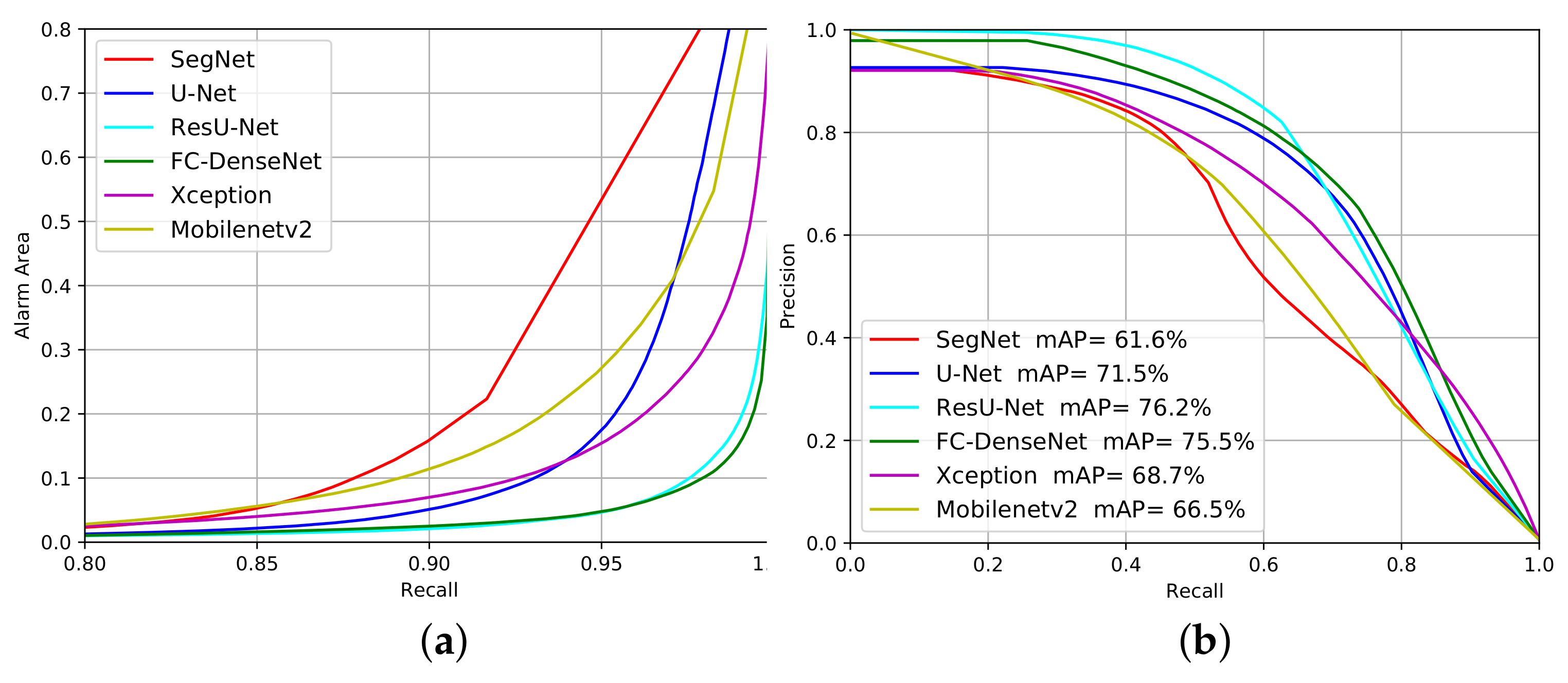
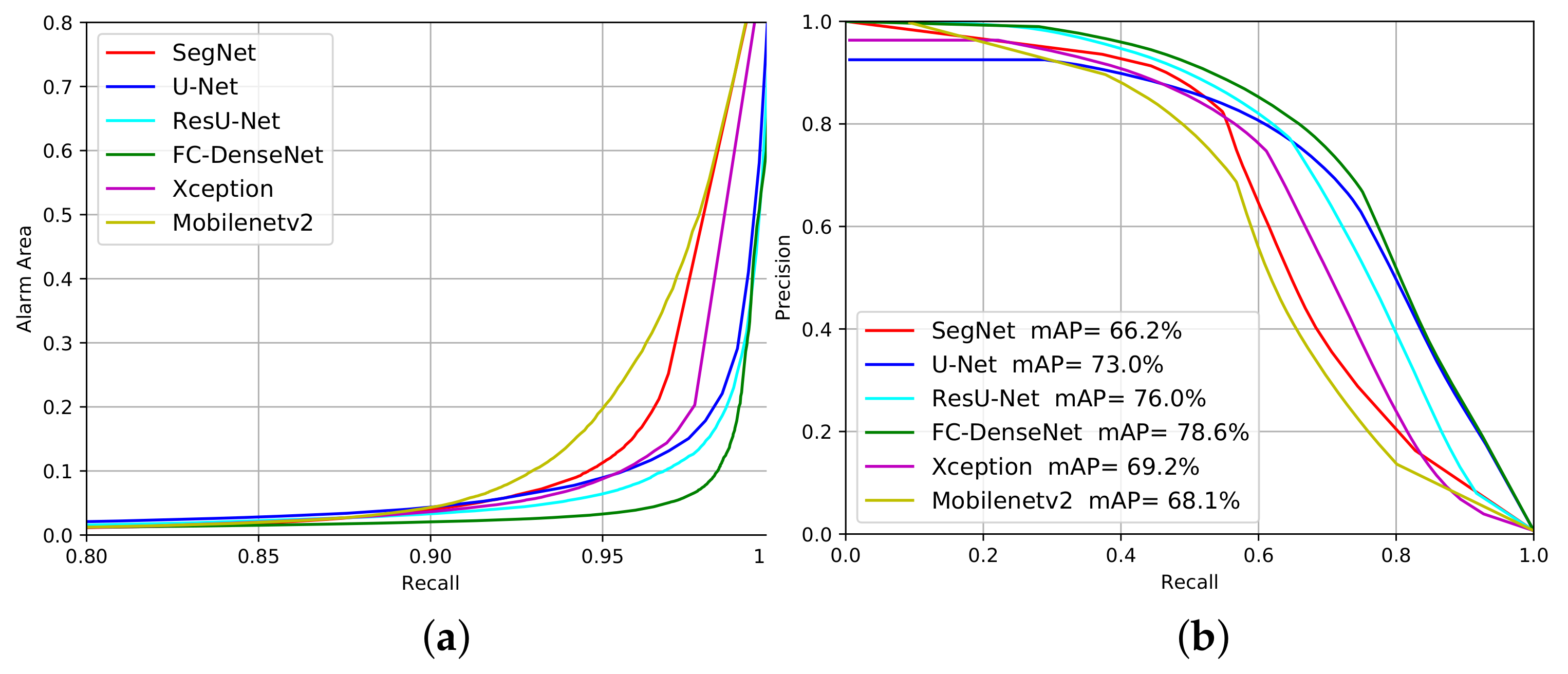
We can evaluate the networks’ performance for different confidence levels of deforestation alarms by changing the probability threshold. Therefore, we built the Alarm Area versus Recall curves (Figure 12a and Figure 13a) and Precision versus Recall curves (Figure 12b and Figure 13b) for the experiments on the Landsat-8 and Sentinel-2 datasets, respectively. The closer each curve is to the coordinates (1,0) and (1,1), respectively, the better the performance will be.
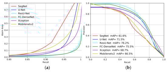
Figure 12.
Evaluation performance of the deforestation approach considering Alarm Area (a) and Precision versus Recall (b) on the Landsat-8 dataset.
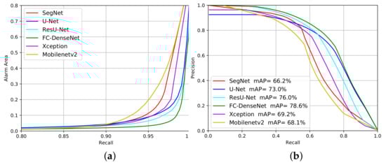
Figure 13.
Evaluation performance of the deforestation approach considering Alarm Area (a) and Precision versus Recall (b) on the Sentinel-2 dataset.
As shown in Figure 12a, all methods, except SegNet and Mobilenetv2, signaled less than 10% of the total imaged area as suspicious of deforestation for a Recall value around 90%. This means that all approaches but SegNet and Mobilenetv2 managed to identify regions that correspond to less than 10% of the imaged area and contain 90% or more of the total deforestation spots. Hence, based on these results, a photo-interpreter could reduce his/her work on less than 10% of the input image that would concentrate more than 90% of all deforestation occurrences.
Fc-DenseNet and ResUnet achieved the best results among all tested network architectures with a Recall higher than 95% for 10% Alarm Area. By this criterion, the U-Net and Xception were between the worst and the best-performing architectures.
Figure 12b also reveal that the Segnet and MobileNetv2 achieved the poorest performance among the evaluated architectures. ResU-Net and FC-DenseNet stood out as the best performers, followed closely by U-Net, while Xception stood behind the first three architectures in the ranking. In comparison with Figure 12a), the inferior Xception performance can be explained by the high number of false positives produced.
The mAP values placed the networks in a similar ranking. ResU-Net, FC-DenseNet and U-Net reached mAP values above 70%, with Xception 1.3% further behind, followed by Mobilenetv2 and SegNet.
The profile in Figure 13a is similar to that of Figure 12a. Again, U-Net, FC-DenseNet, ResU-Net and Xception managed to correctly identify more than 90% of the samples when looking at 10% of the image. It would seem that Segnet and MobileNetv2 also guarantee a lower AA (less than 10%) when Recall values reach 90% for the Sentinel-2 dataset. This result indicates that for all the FCN the omission errors were low and remained almost unchanged with an increase in the threshold.
4.2. Computational Complexity
Table 3 and Table 4 present the average training and inference times measured on the hardware infrastructure described in Section 3.4 for the Landsat-8 and Sentinel-2 datasets, respectively. The training time stands for the median value of over ten runs. The inference time stands for each model’s median prediction time for the whole image.
Table 3.
Average processing time for each FCN for the Landsat Dataset.
Table 4.
Average processing time for each FCN for the Sentinel-2 Dataset.
We trained the networks with the same values of learning rate, batch-size, optimizer, and patch-size, for both datasets and for the architectures described in Table 2. We adopted the same basic design for each architecture, as presented in Section 3.3. The only differences related to the number of spectral bands in each dataset. The training and inference times for Sentinel-2 were longer because the input image was about nine times larger than the Landsat-8 data. We worked with patches () with 50% overlap, which contributed to the high inference time in both datasets. The results shown in Table 3 and Table 4 place the networks in the following increasing order of their respective processing times: (a) MobileNetV2, (b) U-Net, (c) ResU-Net, (d) FC-DenseNet, followed by (e) and (f) Xception and SegNet with the longest processing times.
It is not surprising that MobileNetV2 was the fastest network for training and inference in both databases since this architecture was designed for lightweight devices. What draws attention is that U-Net has shown training times close to those of MobileNetV2, specifically around 10% higher. We also observed that ResUnet achieved a faster training convergence despite its high computational complexity. This was related to the fact that the residual connections present in its architecture facilitate information propagation and convergence speed. The other networks required at least one database more than twice the training time of MobileNetV2. FC-DenseNet followed in the ranking, with SegNet and Xception alternating as the worst architecture in terms of training time.
As for the inference time, MobileNetV2 stood out even more to its counterparts. Even maintaining the same ranking observed for training times, the differences in inference times among the other networks were not that large. However, SegNet and Xception took about twice as long as MobileNetV2 to inference.
5. Discussion
The DL-based techniques investigated in the present paper have promising use in Earth Observation projects such as PRODES that provides the official Brazilian deforestation annual maps in Amazon since 1988. Although diverging from PRODES in several methodological aspects, these techniques can provide deforestation classification products to be consumed in a traditional PRODES auditing process, thus fitting the DL maps to the methodological requirements of the monitoring project.
The PRODES methodology is not based on a pixel-by-pixel classification, but uses (i) visual interpretation and manual vector editing for historical reasons and to provide high accuracy products, (ii) a minimum mapping area to maintain the historical series consistent, and (iii) a mapping scale of 1/75,000, because of the large extension of the Brazilian Amazon, the time-consuming visual interpretation and also because a finer scale would not significantly improve the detection of deforestation polygons higher than the minimal mapping area.
As a result, PRODES may classify small patches of remnant vegetation amid deforested areas as deforestation, and small deforested areas may remain in original forest class. This observation extends to the edges of polygons, which are manually delineated by interpreter vector editing at a fixed mapping scale of 1/75,000.
Although the assessment of the accuracy of DL models by the original PRODES map is relevant, the methodological differences between the two mapping techniques may lead to underestimations in accuracy metrics, as it assumes that the reference map represents the absolute truth at the pixel level.
Another consequence of methodological divergences is an artificial increase of false negatives when using the PRODES minimal mapping unit value as a threshold to filter Deep Learning polygons. Actually, the pixel-by-pixel approach tends to increase polygon fragmentation compared to the PRODES reference. A PRODES polygon larger than the minimum area might be modeled in the form of several fragments smaller than the minimum area, which would improperly exclude part of the set of polygons that were correctly detected.
To neutralize the impact of these divergences on accuracy metrics, the PRODES team of senior analysts conducted an unprecedented experiment of complete auditing of the DL maps that used ResU-Net network on data of both satellites. All PRODES protocol requirements were respected. This auditing allowed (i) to estimate accuracy for DL maps using the final audited PRODES map that would be derived as the reference, (ii) to compare these estimations to the accuracy metrics reported in Section 4.1, based on classical pixel-by-pixel comparison. In addition, this assessment contributed to evaluate the potential of operational use of DL mapping as products to be consumed in PRODES.
The analysts segmented the ResU-Net classified pixels with deforestation probability higher or equal to 0.5 and selected polygons higher than 1 hectare. Visual evaluation, edition and reclassification were performed by one PRODES senior analyst and systematically checked by other analyst, in the entire observed area and for all mapped polygons. During this auditing process, the analysts used the images of the mapping year and of the two precedent years to evaluate the cover change based on tone, color, form, texture and context. This allowed them to keep, add or delete deforestation polygons in a free edition process. The analysts followed the rigorous PRODES protocol to reach the same mapping requirements. After auditing, only polygons higher than 6.25 ha were maintained in the analysis to meet the PRODES standards. The overall accuracy, -score, Recall and Precision were estimated for the DL maps, considering the audited maps as the new PRODES reference.
The estimated accuracy metrics for each satellite are presented in Table 5. As expected, the values increased or remained stable. Despite an unchanged Recall of 62.2%, the Landsat-based map presented a precision higher than 99% according to PRODES auditing. As PRODES considers false positive the most expansive error in deforestation monitoring, this result sounds positive. The accuracy estimates from Sentinel-based map showed a substantial increase in both precision and recall, reaching 82.3% and 74.2% respectively, which positively impacted the -score. The omission area mapped during the auditing process reached 12.5 km and 6.2 km for Landsat and Sentinel maps, respectively. These results mean that the edition effort of original DL maps was mainly related to omission mapping in Landsat-based product, while it was substantial in removing false-positives in Sentinel. This might be explained by the fact that the samples used in model training have been collected in the official deforestation PRODES map based on Landsat images. Such samples would thus present some class divergences when used in finer spatial resolution images.
Table 5.
Accuracy metrics for ResU-Net Landsat and Sentinel maps of deforestation increment using the audited maps as reference (in %). In bold, the values that substantially increased in relation to metrics estimated without auditing. The auditing process was performed at National Institute for Space Research (INPE) by senior PRODES analysts.
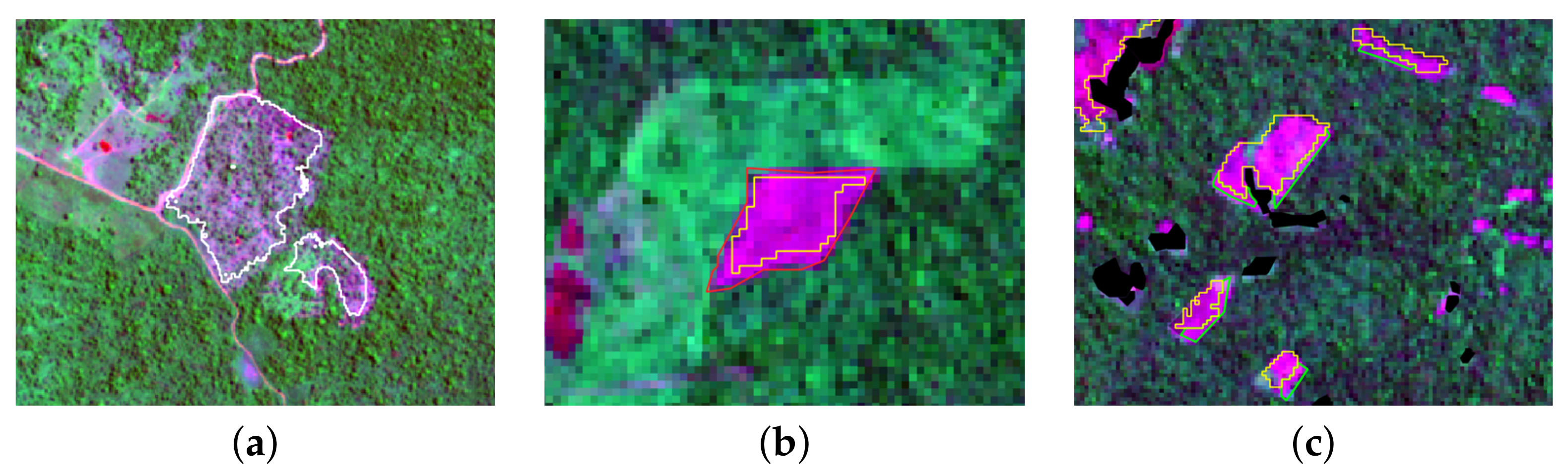
The divergences between DL and audited maps, after filtering by the minimal mapping unit (>6.25 ha), can be represented in two main categories. The first one is detection errors, which are model-dependent and encompass false-positives and false-negatives. The false-positives were almost only observed in Sentinel audited map, and mainly concerned forest polygons that suffered degradation (88.8%), which process generally precedes deforestation (Figure 14a). The higher area of false-positives in Sentinel might be the result of finer spatial resolution, which could have enhanced vegetation changes in the model but not in visual inspection at a 1/75,000 scale. After checking, we noticed that more than 90% of these Sentinel false positives have been classified as deforestation on Landsat DL map, confirming that the higher resolution could have led to this divergence. The false negatives were mainly related to internal proximity to polygon border, as the estimated probability could not reach the 0.5 threshold value, at the contrary of the core area of the polygon (Figure 14b). This might be explained by the model conservatism in detecting deforestation and by delineation divergences of the analyst at the 1/75,000 scale for visual detection and manual mapping. Additionally, we noticed that the smaller was the deforested polygon area, the higher was the omission rate in the model. Recall was significantly reduced to low values 21.9% and 42.1%, respectively for Landsat and Sentinel maps, when only considering lower than 6.25 ha polygons. The second category of errors is derived from shifts between images and PRODES deforestation mask data. It often concerns a maximum of two pixels along part of the polygon border (Figure 14c).

Figure 14.
Main error types in Deep Learning audited maps. (a) False positive: degradation polygon (white line) detected as deforestation; (b) False negative related to model conservatism on polygon borders (detected deforestation in yellow line and false negative complement in red line); and (c) Shifts between images (detected deforestation in yellow line and false negative complement in green line).
To estimate the effective impact of satellite data source on the final PRODES maps, when derived from DL techniques, we compared the total deforestation area detected between the two maps, after auditing. The area reached 32.9 km and 23.7 km, respectively for Landsat and Sentinel. This difference is probably related to the higher spatial resolution in Sentinel that would tend to increase polygon fragmentation and improperly exclude part of the set of polygons that were correctly detected when applying the minimal mapping unit filter, compared to Landsat map. A spatial union of the two audited maps showed that 50.2% of the total area of Landsat and Sentinel final deforestation polygons matched. A total of 62.8% of Landsat derived polygons matched with Sentinel ones and 71.5% of the Sentinel polygons matched with Landsat ones. These results showed that Landsat-based DL detection presented a higher potential to be used as a draft in PRODES mapping, in relation to Sentinel product, when using Landsat-based sampling and the PRODES minimal mapping unit.
This unprecedented experiment showed a substantial improvement of accuracy metrics for both Landsat and Sentinel ResU-Net maps in relation to classic estimation in Section 4.1, when considering PRODES auditing. These results indicate that fully convolutional networks, in particular ResU-Net are promising tools to provide a first draft for the PRODES project, but auditing efforts might focus on omissions that presented a significantly higher rate than false positives principally in Landsat-based maps.
6. Conclusions
In this work, we compared six fully convolutional architectures (U-Net, ResU-Net, SegNet, FC-DenseNet and the Xception and MobileNetV2 variants of DeepLabv3+) for detecting deforestation in the Brazilian Amazon rain forest from Landsat-8 and Sentinel-2 image pairs.
We evaluated the networks’ performance based on different accuracy metrics, computational complexity, and visual assessment. The analysis also considered different confidence levels of deforestation alarms and their implications in terms of false negatives. We did it by varying the probability threshold above which we regarded a pixel as belonging to the class deforestation and recording the corresponding false-positive vs. false-negative values.
The study revealed the potential of the tested networks as an automatic alternative to deforestation mapping programs for the Amazon region that still involve a lot of visual interpretation.
ResU-Net consistently presented the best accuracy among all tested networks, being closely followed by FC-DenseNet. The assessment of how the relation of false-positives vs. false-negatives behaved for different probability thresholds also indicated similar performances of these two networks, but again with ResU-Net’s slight superiority.
As for the associated computational complexity, U-Net was only surpassed by the MobileNetV2, which on the other hand, together with Segnet, achieved the worst accuracy values throughout our experiments.
The experiments on Landsat-8 and Sentinel-2 data led to similar conclusions regarding the networks’ relative performance.
In sum, throughout our experiments, ResU-Net consistently presented the best tradeoff between accuracy and training/inference times. On the other hand, MobileNetV2 and especially Segnet presented the worst results among the evaluated networks.
The Brazilian Amazon biome covers 4.2 million km, has around 2500 tree species and other 30,000 plant species, and is far from being a homogeneous forest. The study presented here constitutes a step towards making the monitoring of the Amazon rainforest more agile, less subjective, and more accurate. Definitive and generally valid conclusions regarding the pros and cons of automatic mapping methods require further studies using data that represents all this diversity. We will be moving towards this goal in the continuation of this research.
Author Contributions
D.L.T. and R.Q.F. conceptualized and designed the search of references and structured literature collections into the original draft; D.L.T., P.J.S.V. and D.E.S. data curation; D.L.T. and J.N.T. software; and D.L.T., R.Q.F., D.E.S., J.M.J., C.A. writing—review and editing. All authors have read and agreed to the published version of the manuscript.
Funding
The authors thank the support from CNPq process 444418/2018-0 as support of INPE, CAPES, FINEP, and FAPERJ.
Informed Consent Statement
Not applicable.
Data Availability Statement
The data presented in this study are openly available in the USGS archives and Copernicus Open Access Hub at https://earthexplorer.usgs.gov/ (accessed on 18 July 2021) and https://scihub.copernicus.eu/dhus/#/home (accessed on 18 July 2021), respectively.
Acknowledgments
The authors thank the support from CNPq, CAPES, FINEP and FAPERJ.
Conflicts of Interest
The authors declare no conflict of interest.
References
- Davidson, E.A.; de Araújo, A.C.; Artaxo, P.; Balch, J.K.; Brown, I.F.; Bustamante, M.M.; Coe, M.T.; DeFries, R.S.; Keller, M.; Longo, M.; et al. The Amazon basin in transition. Nature 2012, 481, 321–328. [Google Scholar] [CrossRef] [PubMed]
- De Almeida, C.A. Estimativa da Area e do Tempo de Permanência da Vegetação Secundaria na Amazônia Legal por Meio de Imagens Landsat/TM. 2009. Available online: http://mtc-m16c.sid.inpe.br/col/sid.inpe.br/mtc-m18@80/2008/11.04.18.45/doc/publicacao.pdf (accessed on 18 July 2021).
- Fearnside, P.M.; Righi, C.A.; de Alencastro Graça, P.M.L.; Keizer, E.W.; Cerri, C.C.; Nogueira, E.M.; Barbosa, R.I. Biomass and greenhouse-gas emissions from land-use change in Brazil’s Amazonian “arc of deforestation”: The states of Mato Grosso and Rondônia. For. Ecol. Manag. 2009, 258, 1968–1978. [Google Scholar] [CrossRef]
- Junior, C.H.S.; Pessôa, A.C.; Carvalho, N.S.; Reis, J.B.; Anderson, L.O.; Aragão, L.E. The Brazilian Amazon deforestation rate in 2020 is the greatest of the decade. Nat. Ecol. Evol. 2021, 5, 144–145. [Google Scholar] [CrossRef] [PubMed]
- Almeida, C.A.; Maurano, L.E.P. Methodology for Forest Monitoring used in PRODES and DETER Projects; INPE: São José dos Campos, Brazil, 2021. [Google Scholar]
- Diniz, C.G.; de Almeida Souza, A.A.; Santos, D.C.; Dias, M.C.; da Luz, N.C.; de Moraes, D.R.V.; Maia, J.S.; Gomes, A.R.; da Silva Narvaes, I.; Valeriano, D.M.; et al. DETER-B: The new Amazon near real-time deforestation detection system. IEEE J. Sel. Top. Appl. Earth Obs. Remote Sens. 2015, 8, 3619–3628. [Google Scholar] [CrossRef]
- Rogan, J.; Miller, J.; Wulder, M.; Franklin, S. Integrating GIS and remotely sensed data for mapping forest disturbance and change. Underst. For. Disturb. Spat. Pattern Remote Sens. GIS Approaches 2006, 133–172. [Google Scholar] [CrossRef]
- Mancino, G.; Nolè, A.; Ripullone, F.; Ferrara, A. Landsat TM imagery and NDVI differencing to detect vegetation change: Assessing natural forest expansion in Basilicata, southern Italy. Ifor.-Biogeosci. For. 2014, 7, 75. [Google Scholar] [CrossRef] [Green Version]
- Hansen, M.C.; Loveland, T.R. A review of large area monitoring of land cover change using Landsat data. Remote Sens. Environ. 2012, 122, 66–74. [Google Scholar] [CrossRef]
- Prakash, A.; Gupta, R. Land-use mapping and change detection in a coal mining area-a case study in the Jharia coalfield, India. Int. J. Remote Sens. 1998, 19, 391–410. [Google Scholar] [CrossRef]
- Asner, G.P.; Keller, M.; Pereira, R., Jr.; Zweede, J.C. Remote sensing of selective logging in Amazonia: Assessing limitations based on detailed field observations, Landsat ETM+, and textural analysis. Remote Sens. Environ. 2002, 80, 483–496. [Google Scholar] [CrossRef]
- Lu, D.; Mausel, P.; Brondizio, E.; Moran, E. Change detection techniques. Int. J. Remote Sens. 2004, 25, 2365–2401. [Google Scholar] [CrossRef]
- Nelson, R.F. Detecting forest canopy change due to insect activity using Landsat MSS. Photogramm. Eng. Remote Sens. 1983, 49, 1303–1314. [Google Scholar]
- Zhu, Z.; Woodcock, C.E. Continuous change detection and classification of land cover using all available Landsat data. Remote Sens. Environ. 2014, 144, 152–171. [Google Scholar] [CrossRef] [Green Version]
- Im, J.; Jensen, J.R. A change detection model based on neighborhood correlation image analysis and decision tree classification. Remote Sens. Environ. 2005, 99, 326–340. [Google Scholar] [CrossRef]
- Schneider, A. Monitoring land cover change in urban and peri-urban areas using dense time stacks of Landsat satellite data and a data mining approach. Remote Sens. Environ. 2012, 124, 689–704. [Google Scholar] [CrossRef]
- Huang, C.; Song, K.; Kim, S.; Townshend, J.R.; Davis, P.; Masek, J.G.; Goward, S.N. Use of a dark object concept and support vector machines to automate forest cover change analysis. Remote Sens. Environ. 2008, 112, 970–985. [Google Scholar] [CrossRef]
- Townshend, J.; Huang, C.; Kalluri, S.; Defries, R.; Liang, S.; Yang, K. Beware of per-pixel characterization of land cover. Int. J. Remote Sens. 2000, 21, 839–843. [Google Scholar] [CrossRef] [Green Version]
- Khan, S.H.; He, X.; Porikli, F.; Bennamoun, M. Forest change detection in incomplete satellite images with deep neural networks. IEEE Trans. Geosci. Remote Sens. 2017, 55, 5407–5423. [Google Scholar] [CrossRef]
- Mou, L.; Bruzzone, L.; Zhu, X.X. Learning Spectral-Spatial-Temporal Features via a Recurrent Convolutional Neural Network for Change Detection in Multispectral Imagery. IEEE Trans. Geosci. Remote Sens. 2019, 57, 924–935. [Google Scholar] [CrossRef] [Green Version]
- Liu, Y.; Chen, X.; Wang, Z.; Wang, Z.J.; Ward, R.K.; Wang, X. Deep learning for pixel-level image fusion: Recent advances and future prospects. Inf. Fusion 2018, 42, 158–173. [Google Scholar] [CrossRef]
- Daudt, R.C.; Le Saux, B.; Boulch, A.; Gousseau, Y. Urban change detection for multispectral earth observation using convolutional neural networks. In Proceedings of the IGARSS 2018—2018 IEEE International Geoscience and Remote Sensing Symposium, Valencia, Spain, 22–27 July 2018; IEEE: New York, NY, USA, 2018; pp. 2115–2118. [Google Scholar]
- Ortega Adarme, M.; Queiroz Feitosa, R.; Nigri Happ, P.; Aparecido De Almeida, C.; Rodrigues Gomes, A. Evaluation of deep learning techniques for deforestation detection in the Brazilian Amazon and cerrado biomes from remote sensing imagery. Remote Sens. 2020, 12, 910. [Google Scholar] [CrossRef] [Green Version]
- Long, J.; Shelhamer, E.; Darrell, T. Fully Convolutional Networks for Semantic Segmentation. CoRR 2014 . Available online: https://arxiv.org/pdf/1411.4038.pdf (accessed on 18 July 2021).
- Caye Daudt, R.; Le Saux, B.; Boulch, A. Fully Convolutional Siamese Networks for Change Detection. In Proceedings of the 2018 25th IEEE International Conference on Image Processing (ICIP), Athens, Greece, 7–10 October 2018; pp. 4063–4067. [Google Scholar]
- De Bem, P.P.; de Carvalho Junior, O.A.; Fontes Guimarães, R.; Trancoso Gomes, R.A. Change Detection of Deforestation in the Brazilian Amazon Using Landsat Data and Convolutional Neural Networks. Remote Sens. 2020, 12, 901. [Google Scholar] [CrossRef] [Green Version]
- Zhang, C.; Yue, P.; Tapete, D.; Jiang, L.; Shangguan, B.; Huang, L.; Liu, G. A deeply supervised image fusion network for change detection in high resolution bi-temporal remote sensing images. ISPRS J. Photogramm. Remote Sens. 2020, 166, 183–200. [Google Scholar] [CrossRef]
- Badrinarayanan, V.; Handa, A.; Cipolla, R. SegNet: A Deep Convolutional Encoder-Decoder Architecture for Robust Semantic Pixel-Wise Labelling. CoRR 2015. Available online: https://arxiv.org/pdf/1511.00561.pdf (accessed on 18 July 2021).
- Ronneberger, O.; Fischer, P.; Brox, T. U-Net: Convolutional Networks for Biomedical Image Segmentation. CoRR 2015. Available online: https://arxiv.org/pdf/1505.04597.pdf (accessed on 18 July 2021).
- Zhang, Z.; Liu, Q.; Wang, Y. Road extraction by deep residual u-net. IEEE Geosci. Remote Sens. Lett. 2018, 15, 749–753. [Google Scholar] [CrossRef] [Green Version]
- He, K.; Zhang, X.; Ren, S.; Sun, J. Deep residual learning for image recognition. In Proceedings of the IEEE Conference on Computer Vision and Pattern Recognition, Las Vegas, NV, USA, 26 June–1 July 2016; pp. 770–778. [Google Scholar]
- Jégou, S.; Drozdzal, M.; Vázquez, D.; Romero, A.; Bengio, Y. The One Hundred Layers Tiramisu: Fully Convolutional DenseNets for Semantic Segmentation. In Proceedings of the 2017 IEEE Conference on Computer Vision and Pattern Recognition Workshops (CVPRW), Honolulu, HI, USA, 21–26 June 2017; pp. 1175–1183. [Google Scholar]
- Huang, G.; Liu, Z.; Van Der Maaten, L.; Weinberger, K.Q. Densely Connected Convolutional Networks. In Proceedings of the IEEE Conference on Computer Vision and Pattern Recognition (CVPR), Honolulu, HI, USA, 21–27 June 2017; pp. 2261–2269. [Google Scholar]
- Lobo Torres, D.; Queiroz Feitosa, R.; Nigri Happ, P.; Elena Cué La Rosa, L.; Marcato Junior, J.; Martins, J.; Olã Bressan, P.; Gonçalves, W.N.; Liesenberg, V. Applying fully convolutional architectures for semantic segmentation of a single tree species in urban environment on high resolution UAV optical imagery. Sensors 2020, 20, 563. [Google Scholar] [CrossRef] [Green Version]
- Chen, L.; Zhu, Y.; Papandreou, G.; Schroff, F.; Adam, H. Encoder-Decoder with Atrous Separable Convolution for Semantic Image Segmentation. CoRR 2018. Available online: https://arxiv.org/pdf/1802.02611.pdf (accessed on 18 July 2021).
- Chollet, F. Xception: Deep Learning with Depthwise Separable Convolutions. CoRR 2016. Available online: https://openaccess.thecvf.com/content_cvpr_2017/papers/Chollet_Xception_Deep_Learning_CVPR_2017_paper.pdf (accessed on 18 July 2021).
- Chen, L.; Papandreou, G.; Schroff, F.; Adam, H. Rethinking Atrous Convolution for Semantic Image Segmentation. CoRR 2017. Available online: https://arxiv.org/pdf/1706.05587.pdf (accessed on 18 July 2021).
- Sandler, M.; Howard, A.G.; Zhu, M.; Zhmoginov, A.; Chen, L. Inverted Residuals and Linear Bottlenecks: Mobile Networks for Classification, Detection and Segmentation. CoRR 2018. Available online: https://arxiv.org/pdf/1801.04381.pdf (accessed on 18 July 2021).
- Maurano, L.; Escada, M.; Renno, C.D. Spatial deforestation patterns and the accuracy of deforestation mapping for the Brazilian Legal Amazon. Ciência Florest. 2019, 29, 1763–1775. [Google Scholar] [CrossRef]
- Keras. Available online: https://keras.io/getting_started/ (accessed on 18 July 2021).
- Sokolova, M.; Japkowicz, N.; Szpakowicz, S. Beyond Accuracy, F-Score and ROC: A Family of Discriminant Measures for Performance Evaluation. In Proceedings of the Australasian Joint Conference on Artificial Intelligence, Hobart, Australia, 4–8 December 2006; Springer: Berlin/Heidelberg, Germany, 2006; pp. 1015–1021. [Google Scholar]


Publisher’s Note: MDPI stays neutral with regard to jurisdictional claims in published maps and institutional affiliations. |
© 2021 by the authors. Licensee MDPI, Basel, Switzerland. This article is an open access article distributed under the terms and conditions of the Creative Commons Attribution (CC BY) license (https://creativecommons.org/licenses/by/4.0/).