
Towards Routine Mapping of Crop Emergence within the Season Using the Harmonized Landsat and Sentinel-2 Dataset

 , ,
, ,  ,
,
Abstract
:
1. Introduction
2. Study Area and Data
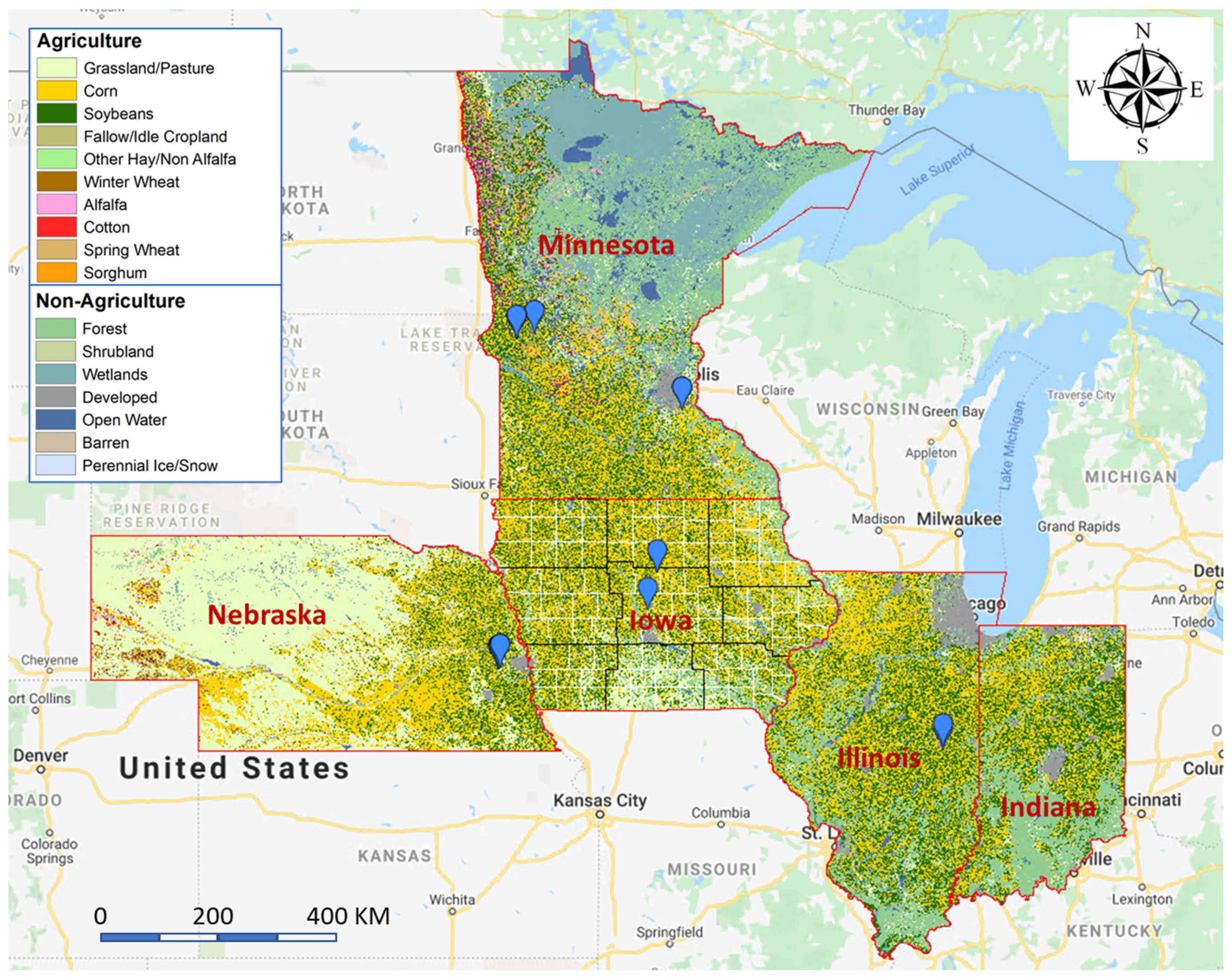
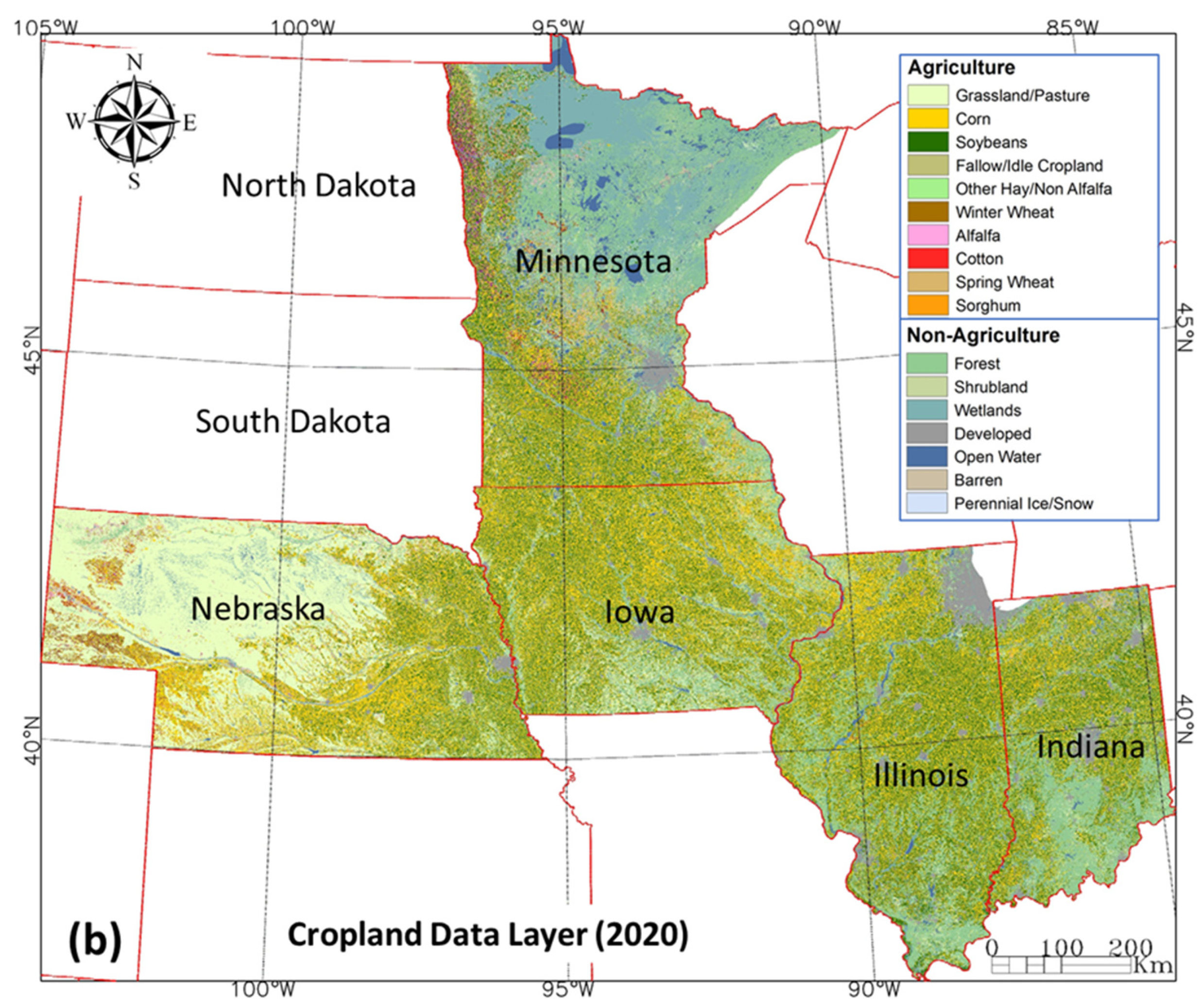
2.1. Study Area
2.2. Data Compilation
2.2.1. Phenocam Observation
2.2.2. HLS Data
2.2.3. NASS Data
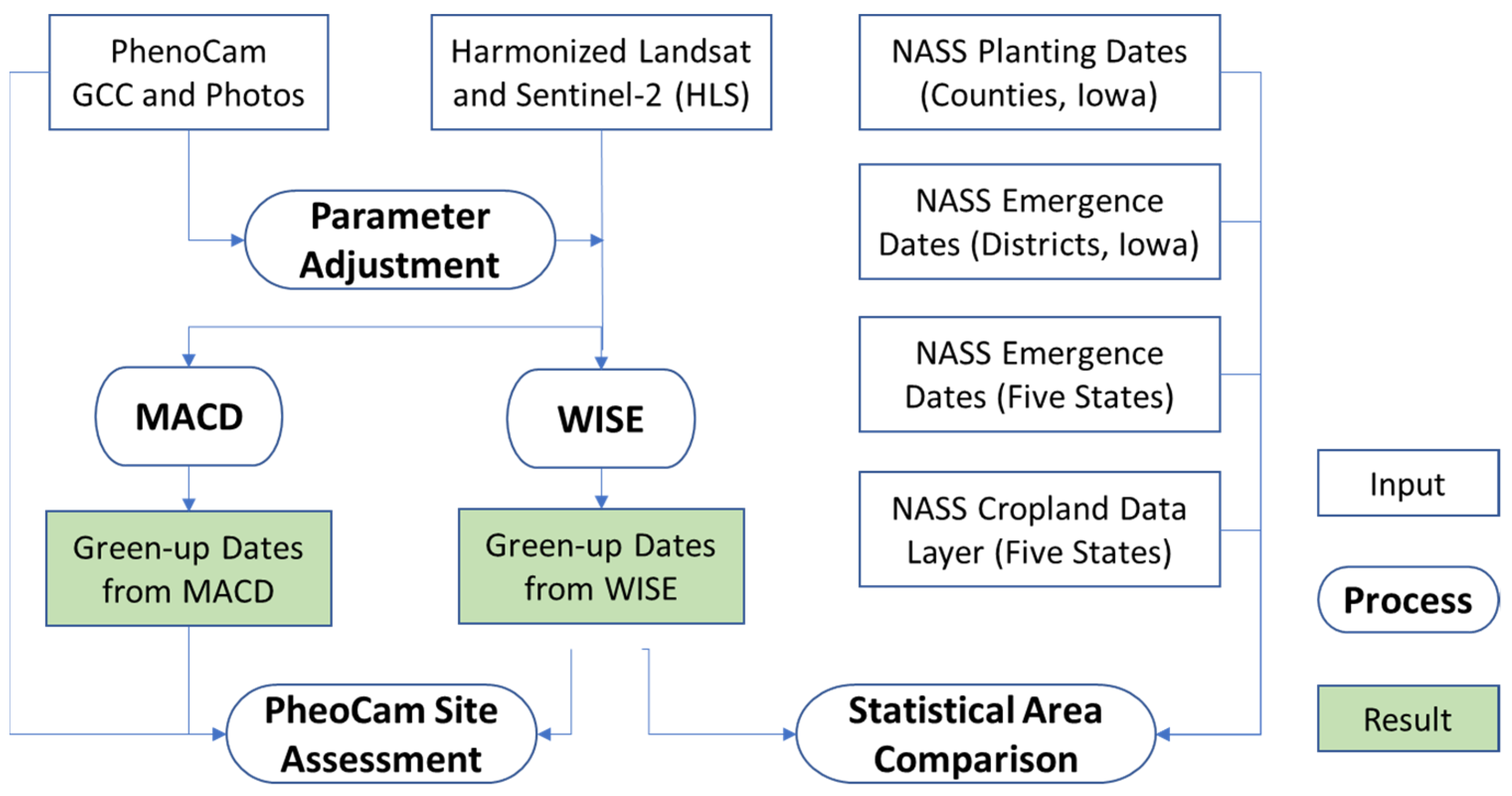
3. Analytical Methods
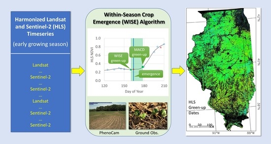
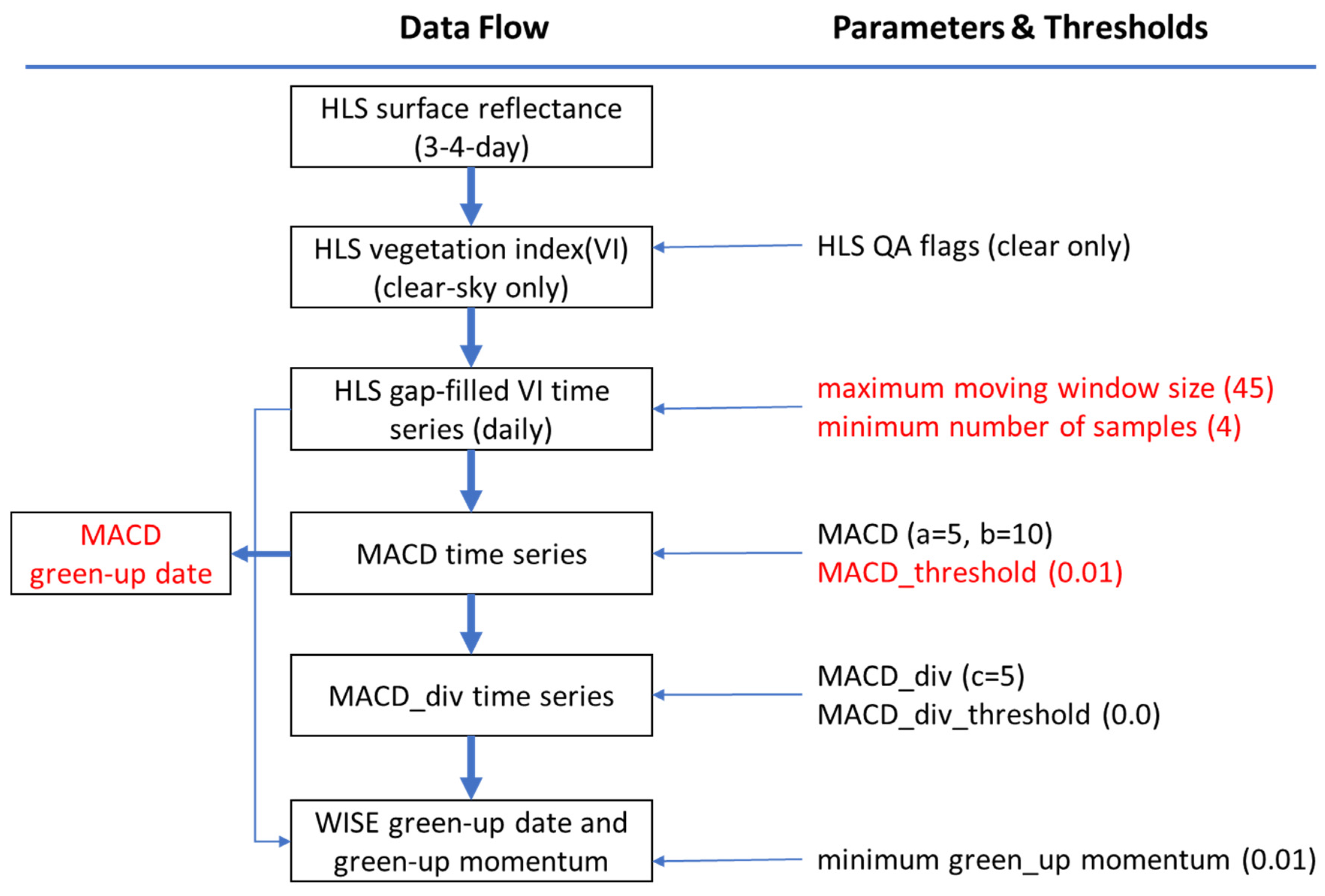
3.1. WISE Algorithm
3.2. Parameter Adjustment for Corn Belt
3.3. Assessment
4. Results
4.1. WISE Parameter Adjustment
4.2. Green-Up Dates at PhenoCam Sites
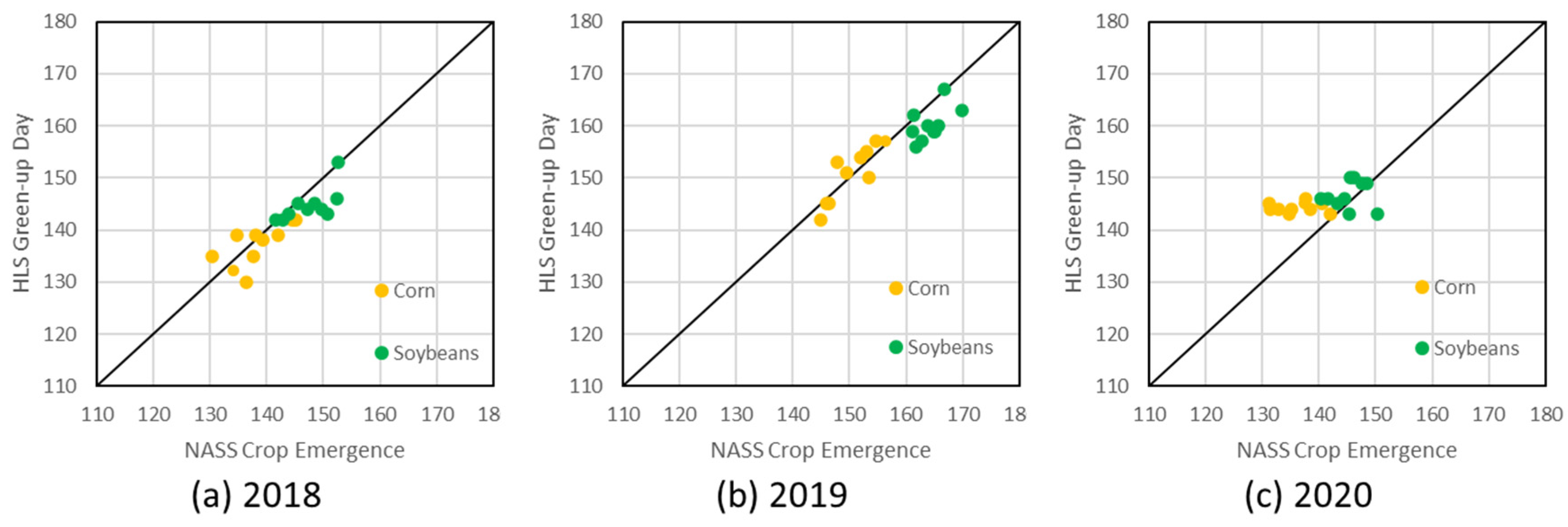
4.3. Assessment at County and District Level in Iowa
4.4. Assessment at State Level
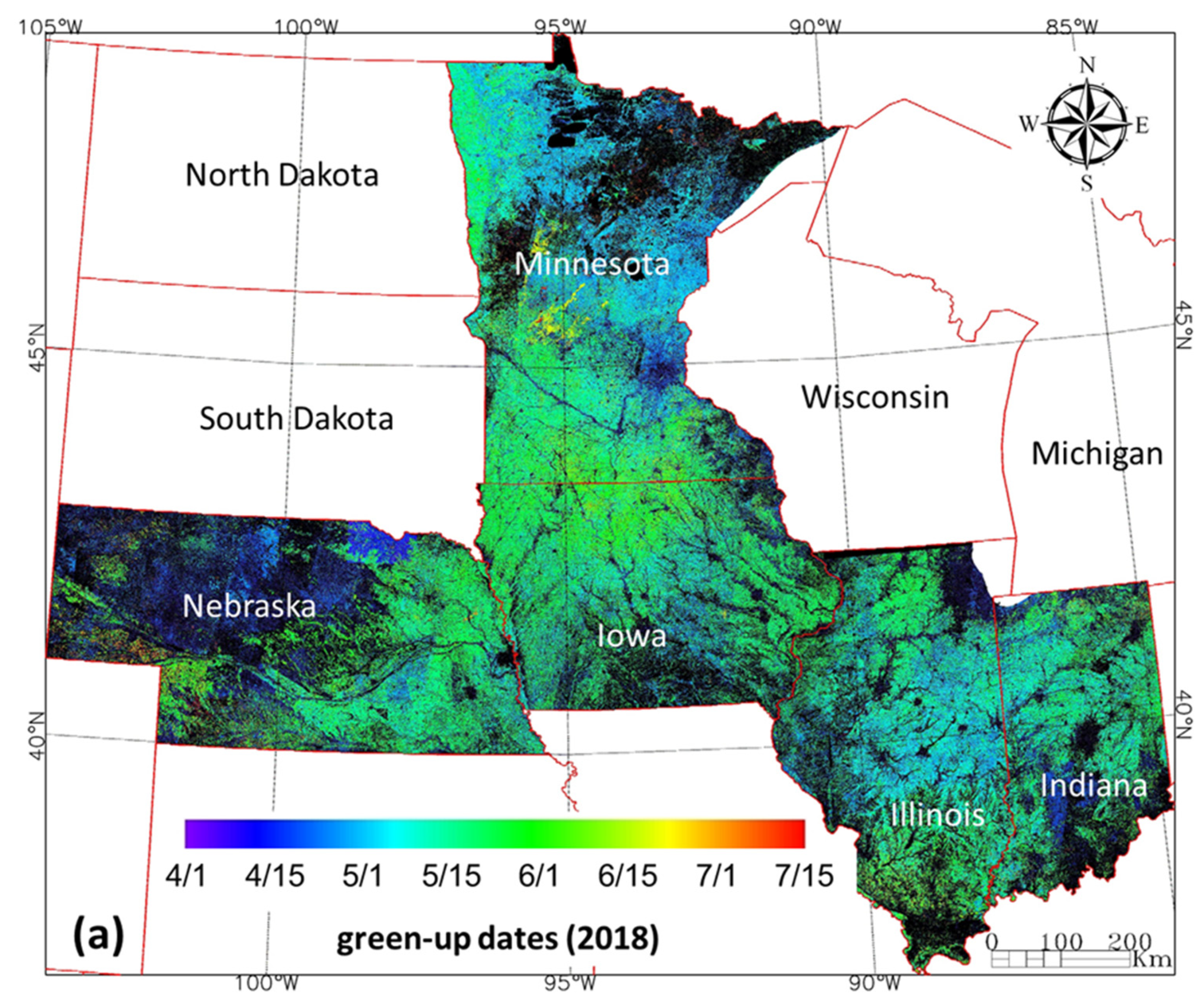
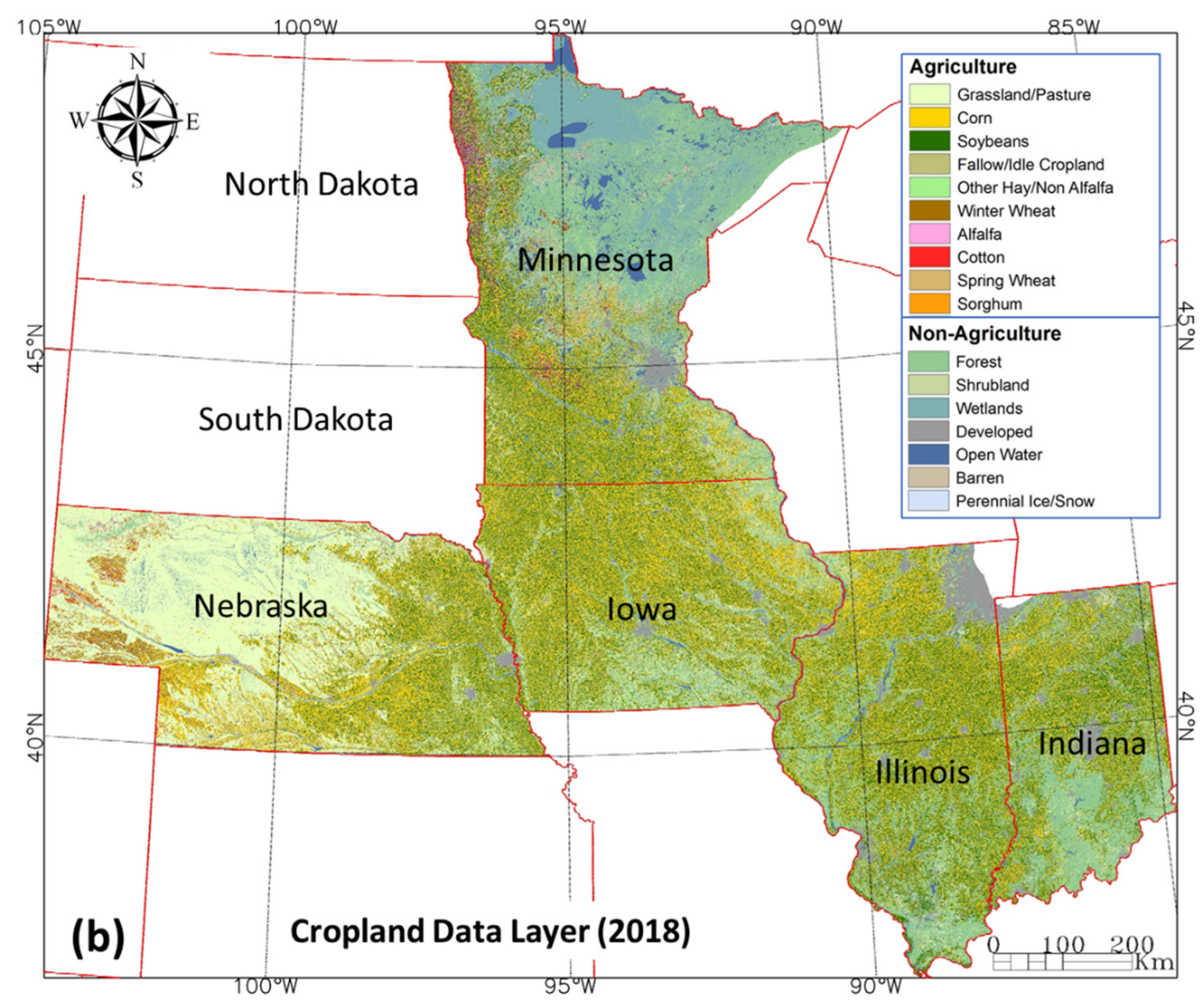
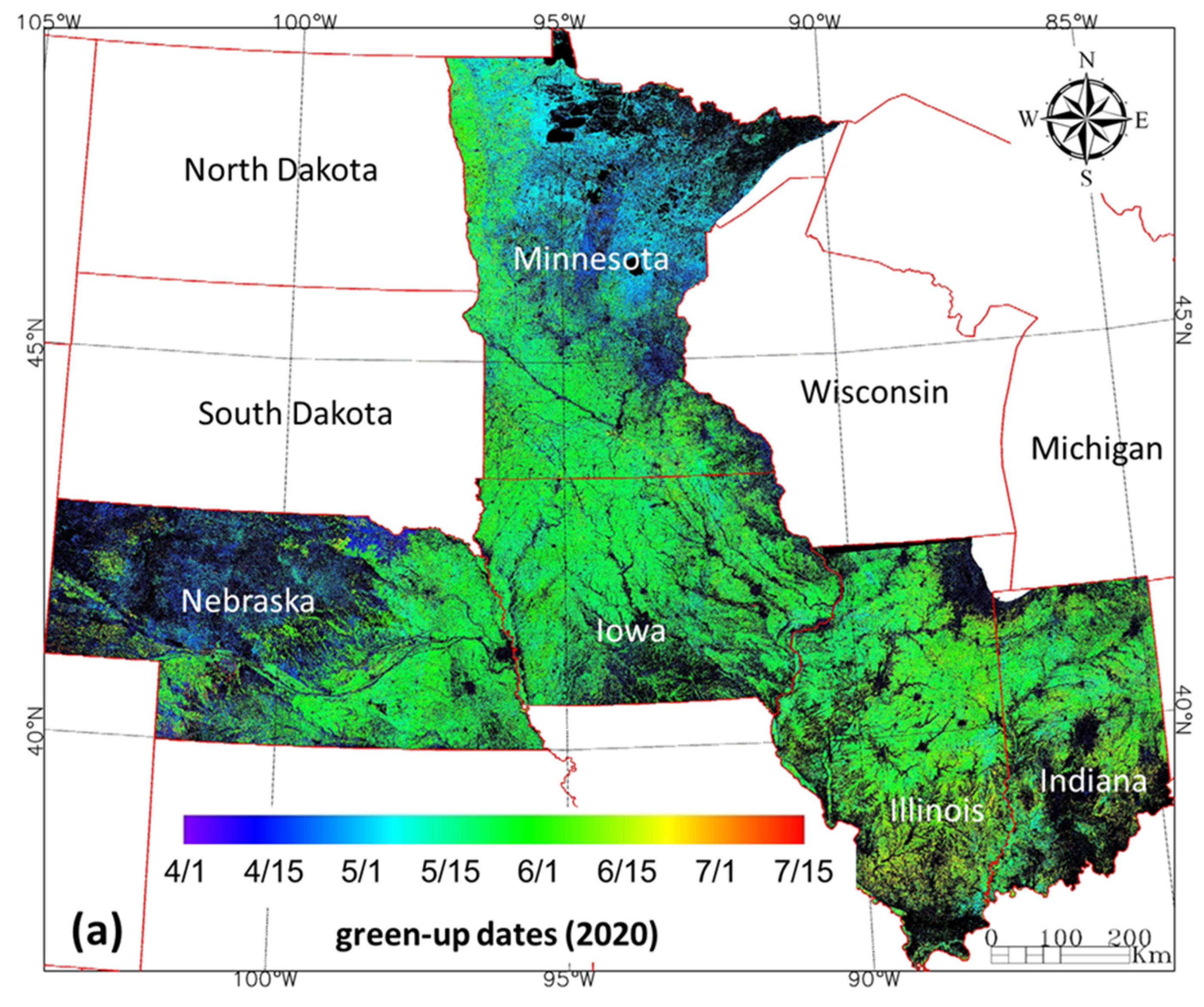
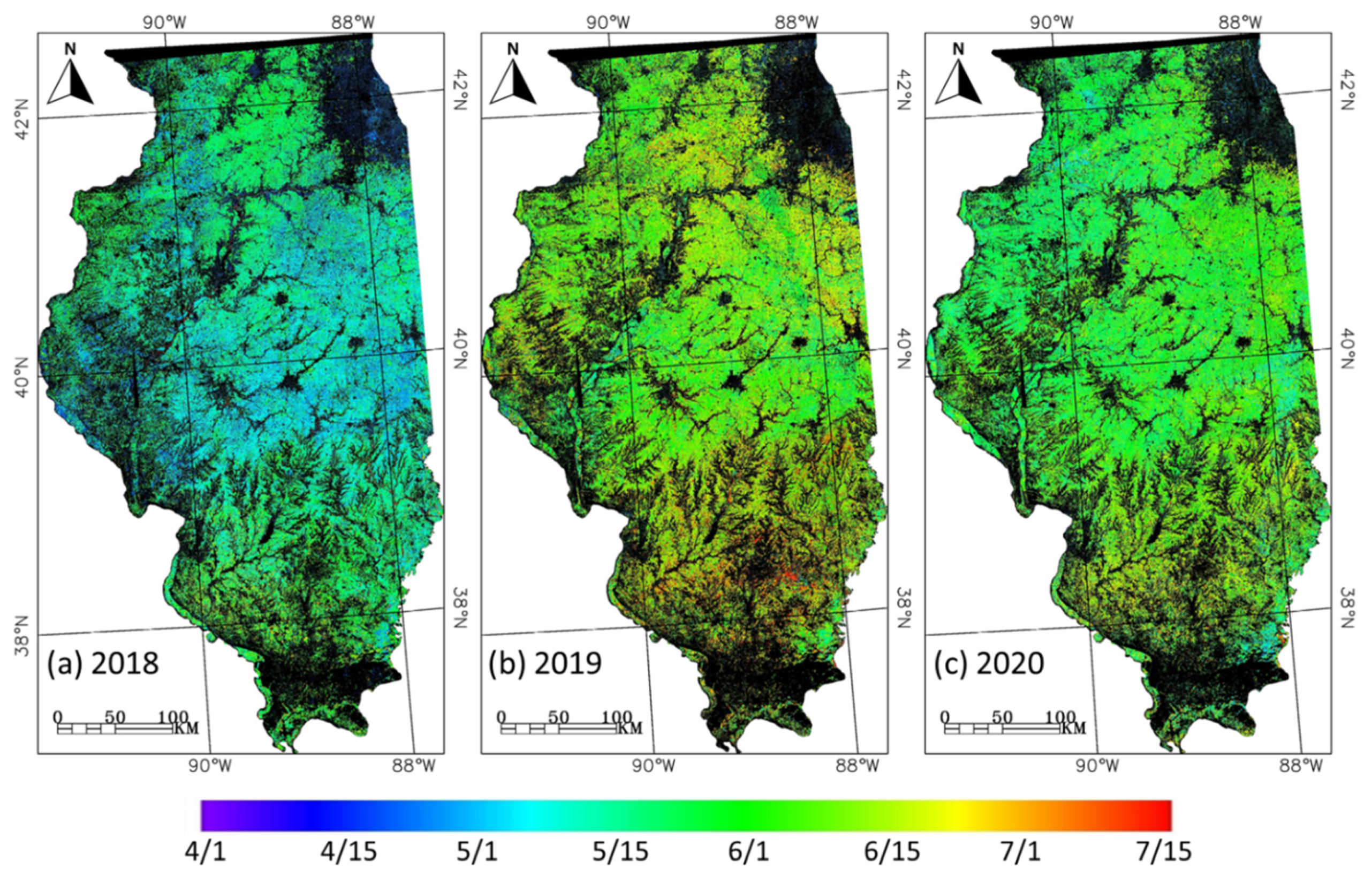
4.5. Green-Up Mapping
5. Discussion
5.1. Algorithm Parameters
5.2. Validation and Comparison
5.3. Challenges on Near-Real-Time Mapping and Future Improvements
6. Conclusions
Author Contributions
Funding
Data Availability Statement
Acknowledgments
Conflicts of Interest
Appendix A

References
- Kucharik, C.J. A Multidecadal Trend of Earlier Corn Planting in the Central USA. Agron. J. 2006, 98, 1544–1550. [Google Scholar] [CrossRef] [Green Version]
- Walthall, C.L.; Hatfield, J.; Backlund, P.; Lengnick, L.; Marshall, E.; Walsh, M.; Adkins, S.; Aillery, M.; Ainsworth, E.A.; Ammann, C.; et al. Climate Change and Agriculture in the United States: Effects and Adaptation; USDA Technical Bulletin 1935; USDA: Washington, DC, USA, 2012; 186p.
- Neild, R.E.; Newman, J.E. Growing Season Characteristics and Requirements in the Corn Belt. NCH-40. Cooperative Extension Service, Purdue University. Available online: https://www.extension.purdue.edu/extmedia/nch/nch-40.html (accessed on 8 November 2021).
- Rosenzweig, C.; Jones, J.W.; Hatfield, J.L.; Ruane, A.C.; Boote, K.; Thorburn, P.; Antle, J.M.; Nelson, G.C.; Porter, C.; Janssen, S.; et al. The Agricultural Model Intercomparison and Improvement Project (AgMIP): Protocols and pilot studies. Agric. For. Meteorol. 2013, 170, 166–182. [Google Scholar] [CrossRef] [Green Version]
- Yang, Y.; Anderson, M.C.; Gao, F.; Wardlow, B.; Hain, C.R.; Otkin, J.A.; Alfieri, J.; Yang, Y.; Sun, L.; Dulaney, W. Field-scale mapping of evaporative stress indicators of crop yield: An application over Mead, NE, USA. Remote Sens. Environ. 2018, 210, 387–402. [Google Scholar] [CrossRef]
- Müller, C.; Elliott, J.; Kelly, D.; Arneth, A.; Balkovic, J.; Ciais, P.; Deryng, D.; Folberth, C.; Hoek, S.; Izaurralde, R.; et al. The Global Gridded Crop Model Intercomparison phase 1 simulation dataset. Sci. Data 2019, 6, 50. [Google Scholar] [CrossRef]
- USDA National Agricultural Statistics Service. Crop Progress Report. Available online: http://www.nass.usda.gov/Publications/National_Crop_Progress/ (accessed on 8 November 2021).
- Zhang, X.; Friedl, M.A.; Schaaf, C.B.; Strahler, A.H.; Hodges, J.C.F.; Gao, F.; Reed, B.C.; Huete, A. Monitoring vegetation phenology using MODIS. Remote Sens. Environ. 2003, 84, 471–475. [Google Scholar] [CrossRef]
- Zhang, X.; Liu, L.; Liu, Y.; Jayavelu, S.; Wang, J.; Moon, M.; Henebry, G.M.; Friedl, M.A.; Schaaf, C.B. Generation and evaluation of the VIIRS land surface phenology product. Remote Sens. Environ. 2018, 216, 212–229. [Google Scholar] [CrossRef]
- Zeng, L.; Wardlow, B.D.; Wang, R.; Shan, J.; Tadesse, T.; Hayes, M.J.; Li, D. A hybrid approach for detecting corn and soybean phenology with time-series MODIS data. Remote Sens. Environ. 2016, 181, 237–250. [Google Scholar] [CrossRef]
- Bolton, D.K.; Gray, J.M.; Melaas, E.K.; Moon, M.; Eklundh, L.; Friedl, M.A. Continental-scale land surface phenology from harmonized Landsat 8 and Sentinel-2 imagery. Remote Sens. Environ. 2020, 240, 111685. [Google Scholar] [CrossRef]
- Taylor, S.D.; Browning, D.M.; Baca, R.A.; Gao, F. Constraints and Opportunities for Detecting Land Surface Phenology in Drylands. J. Remote Sens. 2021, 2021, 9859103. [Google Scholar] [CrossRef]
- Gao, F.; Anderson, M.C.; Zhang, X.; Yang, Z.; Alfieri, J.G.; Kustas, W.P.; Mueller, R.; Johnson, D.M.; Prueger, J.H. Toward mapping crop progress at field scales through fusion of Landsat and MODIS imagery. Remote Sens. Environ. 2017, 188, 9–25. [Google Scholar] [CrossRef] [Green Version]
- Diao, C. Remote sensing phenological monitoring framework to characterize corn and soybean physiological growing stages. Remote Sens. Environ. 2020, 248, 111960. [Google Scholar] [CrossRef]
- Gao, F.; Zhang, X. Mapping Crop Phenology in Near Real-Time Using Satellite Remote Sensing: Challenges and Opportunities. J. Remote Sens. 2021, 2021, 8379391. [Google Scholar] [CrossRef]
- Gao, F.; Anderson, M.; Daughtry, C.; Karnieli, A.; Hively, D.; Kustas, W. A within-season approach for detecting early growth stages in corn and soybean using high temporal and spatial resolution imagery. Remote Sens. Environ. 2020, 242, 111752. [Google Scholar] [CrossRef]
- Liu, L.; Zhang, X.; Yu, Y.; Gao, F.; Yang, Z. Real-Time Monitoring of Crop Phenology in the Midwestern United States Using VIIRS Observations. Remote Sens. 2018, 10, 1540. [Google Scholar] [CrossRef] [Green Version]
- Yan, L.; Roy, D.P. Conterminous United States crop field size quantification from multi-temporal Landsat data. Remote Sens. Environ. 2016, 172, 67–86. [Google Scholar] [CrossRef] [Green Version]
- Gao, F.; Masek, J.; Schwaller, M.; Hall, F. On the blending of the Landsat and MODIS surface reflectance: Predicting daily Landsat surface reflectance. IEEE Trans. Geosci. Remote Sens. 2006, 44, 2207–2218. [Google Scholar] [CrossRef]
- Gao, F.; Masek, J.G.; Wolfe, R.; Huang, C. Building a consistent medium resolution satellite data set using moderate resolution imaging spectroradiometer products as reference. J. Appl. Remote Sens. 2010, 4, 043526. [Google Scholar] [CrossRef]
- Zhu, X.; Cai, F.; Tian, J.; Williams, T.K.-A. Spatiotemporal Fusion of Multisource Remote Sensing Data: Literature Survey, Taxonomy, Principles, Applications, and Future Directions. Remote Sens. 2018, 10, 527. [Google Scholar] [CrossRef] [Green Version]
- Walker, J.J.; De Beurs, K.M.; Wynne, R.H.; Gao, F. Evaluation of Landsat and MODIS data fusion products for analysis of dryland forest phenology. Remote Sens. Environ. 2012, 117, 381–393. [Google Scholar] [CrossRef]
- Zhang, X.; Wang, J.; Henebry, G.M.; Gao, F. Development and evaluation of a new algorithm for detecting 30 m land surface phenology from VIIRS and HLS time series. ISPRS J. Photogramm. Remote Sens. 2020, 161, 37–51. [Google Scholar] [CrossRef]
- Claverie, M.; Ju, J.; Masek, J.G.; Dungan, J.L.; Vermote, E.F.; Roger, J.-C.; Skakun, S.V.; Justice, C. The Harmonized Landsat and Sentinel-2 surface reflectance data set. Remote Sens. Environ. 2018, 219, 145–161. [Google Scholar] [CrossRef]
- Gray, J.; Sulla-Menashe, D.; Friedl, M. User Guide to Collection 6 MODIS Land Cover Dynamics (MCD12Q2) Product. Available online: https://lpdaac.usgs.gov/documents/218/mcd12q2_v6_user_guide.pdf (accessed on 8 November 2021).
- Gao, F.; Anderson, M.C.; Hively, W.D. Detecting Cover Crop End-Of-Season Using VENµS and Sentinel-2 Satellite Imagery. Remote Sens. 2020, 12, 3524. [Google Scholar] [CrossRef]
- Dedieu, G.; Hagolle, O.; Karnieli, A.; Ferrier, P.; Crébassol, P.; Gamet, P.; Desjardins, C.; Yakov, M.; Cohen, M.; Hayun, E. VENµS: Performances and first results after 11 months in orbit. In Proceedings of the 2018 IEEE International Geoscience and Remote Sensing Symposium (IGARSS 2018), Valencia, Spain, 22–27 July 2018. [Google Scholar] [CrossRef]
- USDA National Agricultural Statistics Service. Quick Stats. Available online: https://quickstats.nass.usda.gov/ (accessed on 8 November 2021).
- PhenoCam Network. Available online: https://phenocam.sr.unh.edu/webcam/ (accessed on 8 November 2021).
- The Long-Term Agroecosystem Research (LTAR) Network. Available online: https://ltar.ars.usda.gov (accessed on 8 November 2021).
- Browning, D.M.; Russell, E.S.; Ponce-Campos, G.E.; Kaplan, N.; Richardson, A.D.; Seyednasrollah, B.; Spiegal, S.; Saliendra, N.; Alfieri, J.G.; Baker, J.; et al. Monitoring agroecosystem productivity and phenology at a national scale: A metric assessment framework. Ecol. Indic. 2021, 131, 108147. [Google Scholar] [CrossRef]
- Suyker, A.E.; Verma, S.B. Gross primary production and ecosystem respiration of irrigated and rainfed maize–soybean cropping systems over 8 years. Agric. For. Meteorol. 2012, 165, 12–24. [Google Scholar] [CrossRef] [Green Version]
- Richardson, A.D.; Braswell, B.H.; Hollinger, D.Y.; Jenkins, J.P.; Ollinger, S.V. Near-surface remote sensing of spatial and temporal variation in canopy phenology. Ecol. Appl. 2009, 19, 1417–1428. [Google Scholar] [CrossRef] [PubMed]
- Richardson, A.D.; Hufkens, K.; Milliman, T.; Aubrecht, D.M.; Chen, M.; Gray, J.; Johnston, M.R.; Keenan, T.; Klosterman, S.T.; Kosmala, M.; et al. Tracking vegetation phenology across diverse North American biomes using PhenoCam imagery. Sci. Data 2018, 5, 180028. [Google Scholar] [CrossRef] [PubMed]
- European Space Agency (ESA). Sentinel-2 User Handbook. Available online: https://sentinels.copernicus.eu/documents/247904/685211/Sentinel-2_User_Handbook (accessed on 8 November 2021).
- Roy, D.P.; Wulder, M.A.; Loveland, T.R.; Woodcock, C.E.; Allen, R.G.; Anderson, M.C.; Helder, D.; Irons, J.R.; Johnson, D.M.; Kennedy, R.; et al. Landsat-8: Science and product vision for terrestrial global change research. Remote Sens. Environ. 2014, 145, 154–172. [Google Scholar] [CrossRef] [Green Version]
- The Harmonized Landsat-8 and Sentinel-2 (HLS) Data Product. Available online: https://hls.gsfc.nasa.gov/data/ (accessed on 8 November 2021).
- USDA Farm Service Agency Handbook. Acreage and Compliance Determinations. Available online: https://www.fsa.usda.gov/Internet/FSA_File/2cp16-a1.pdf (accessed on 8 November 2021).
- USDA National Agricultural Statistics Service. Iowa Crop Progress Reports. Available online: https://www.nass.usda.gov/Statistics_by_State/Iowa/Publications/Crop_Progress_&_Condition/ (accessed on 8 November 2021).
- Boryan, C.; Yang, Z.; Mueller, R.; Craig, M. Monitoring US agriculture: The US Department of Agriculture, National Agricultural Statistics Service, Cropland Data Layer Program. Geocarto Int. 2011, 26, 341–358. [Google Scholar] [CrossRef]
- USDA National Agricultural Statistics Service. Cropland Data Layer. Available online: http://www.nass.usda.gov/Research_and_Science/Cropland/SARS1a.php (accessed on 8 November 2021).
- Appel, G. Technical Analysis Power Tools for Active Investors; Financial Times Prentice Hall: Upper Saddle River, NJ, USA, 2005; p. 166. [Google Scholar]
- USDA National Agricultural Statistics Service. Usual Planting and Harvesting Dates for U.S. Field Crops. Available online: https://downloads.usda.library.cornell.edu/usda-esmis/files/vm40xr56k/dv13zw65p/w9505297d/planting-10-29-2010.pdf (accessed on 8 November 2021).
- Iowa Environmental Mesonet. Available online: https://mesonet.agron.iastate.edu/ (accessed on 8 November 2021).
- USDA Farm Service Agency. Crop Acreage Data. Available online: https://www.fsa.usda.gov/Assets/USDA-FSA-Public/usdafiles/NewsRoom/eFOIA/crop-acre-data/zips/2019-crop-acre-data/2019_fsa_acres_jan2020_stlno1.zip (accessed on 8 November 2021).
- Houborg, R.; McCabe, M.F. A Cubesat enabled Spatio-Temporal Enhancement Method (CESTEM) Utilizing Planet, Landsat and MODIS Data. Remote Sens. Environ. 2018, 209, 211–226. [Google Scholar] [CrossRef]
- Planet Lab Inc. Planet Fusion Monitoring Technical Specification. Available online: https://assets.planet.com/docs/Planet_fusion_specification_March_2021.pdf (accessed on 8 November 2021).
- Cheng, Y.; Vrieling, A.; Fava, F.; Meroni, M.; Marshall, M.; Gachoki, S. Phenology of short vegetation cycles in a Kenyan rangeland from PlanetScope and Sentinel-2. Remote Sens. Environ. 2020, 248, 112004. [Google Scholar] [CrossRef]


| State | Corn Production (BU) | Portion in US (%) | Ranking in US | Soybean Production (BU) | Portion in US (%) | Ranking in US |
|---|---|---|---|---|---|---|
| Illinois | 2,131,200,000 | 15.03 | 2 | 604,750,000 | 14.62 | 1 |
| Indiana | 981,750,000 | 6.92 | 5 | 329,440,000 | 7.97 | 4 |
| Iowa | 2,296,200,000 | 16.19 | 1 | 493,960,000 | 11.94 | 2 |
| Minnesota | 1,441,920,000 | 10.17 | 4 | 359,170,000 | 8.69 | 3 |
| Nebraska | 1,790,090,000 | 12.62 | 3 | 294,120,000 | 7.11 | 5 |
| State | Name | Latitude | Longitude | Year | VE (Day) | Crop |
|---|---|---|---|---|---|---|
| arsmnswanlake1 | 45.6845 | −95.7997 | 2018 | 148 | corn | |
| arsmnswanlake1 | 45.6845 | −95.7997 | 2019 | 162 | soybean | |
| arsmnswanlake1 | 45.6845 | −95.7997 | 2020 | 149 | corn | |
| arsmorris1 | 45.6167 | −96.1269 | 2018 | 147 | corn | |
| arsmorris1 | 45.6167 | −96.1269 | 2019 | 170 | soybean | |
| arsmorris1 | 45.6167 | −96.1269 | 2020 | 152 | corn | |
| MN | arsmorris2 | 45.6270 | −96.1270 | 2018 | 139 | wheat |
| arsmorris2 | 45.6270 | −96.1270 | 2019 | 198 | fallow/grass | |
| arsmorris2 | 45.6270 | −96.1270 | 2020 | 148 | corn | |
| rosemountconv | 44.6910 | −93.0576 | 2017 | 159 | soybean | |
| rosemountconv | 44.6910 | −93.0576 | 2018 | 147 | corn | |
| rosemountconv | 44.6910 | −93.0576 | 2019 | 164 | soybean | |
| rosemountconv | 44.6910 | −93.0576 | 2020 | 152 | corn | |
| arscolessouth | 42.4816 | −93.5235 | 2019 | 177 | soybean | |
| arscolessouth | 42.4816 | −93.5235 | 2020 | 136 | corn | |
| IA | arscolesnorth | 42.4884 | −93.5225 | 2019 | 164 | corn |
| arsbrooks10 | 41.9749 | −93.6905 | 2020 | 143 | soybean | |
| arsbrooks11 | 41.9744 | −93.6937 | 2020 | 126 | corn | |
| mead1 | 41.1651 | −96.4766 | 2017 | 128 | corn | |
| mead1 | 41.1651 | −96.4766 | 2018 | 137 | corn | |
| mead1 | 41.1651 | −96.4766 | 2019 | 125 | corn | |
| mead1 | 41.1651 | −96.4766 | 2020 | 122 | corn | |
| mead2 | 41.1649 | −96.4701 | 2017 | 134 | corn | |
| mead2 | 41.1649 | −96.4701 | 2018 | 141 | soybean | |
| NE | mead2 | 41.1649 | −96.4701 | 2019 | 131 | corn |
| mead2 | 41.1649 | −96.4701 | 2020 | 141 | soybean | |
| mead3 | 41.1797 | −96.4397 | 2017 | 135 | corn | |
| mead3 | 41.1797 | −96.4397 | 2018 | 141 | soybean | |
| mead3 | 41.1797 | −96.4397 | 2019 | 133 | corn | |
| mead3 | 41.1797 | −96.4397 | 2020 | 142 | soybean | |
| uiefsorghum | 40.0065 | −88.2032 | 2019 | 144 | soybean | |
| uiefsorghum | 40.0065 | −88.2032 | 2020 | 145 | sorghum | |
| IL | uiefmaize2 | 40.0628 | −88.1961 | 2019 | 152 | soybean |
| uiefmaize2 | 40.0628 | −88.1961 | 2020 | 148 | corn |
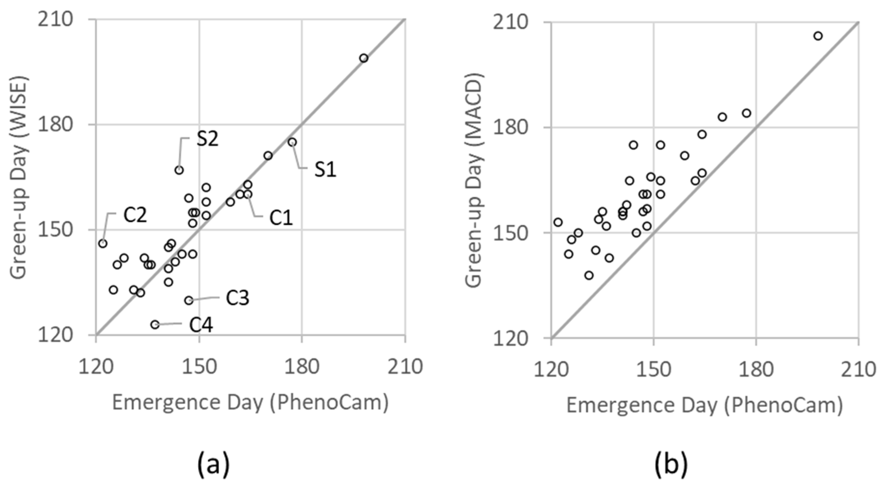
| Statistical Metrics | WISE | MACD |
|---|---|---|
| Mean Difference (MD, days) | 3.0 | 14.1 |
| Mean Absolute Difference (MAD, days) | 6.6 | 14.1 |
| Root Mean Square Error (RMSE, days) | 9.0 | 15.8 |
| Coefficient of determination (R2) | 0.72 | 0.79 |
| Year | State | Corn | Soybeans |
|---|---|---|---|
| 2018 | Iowa | −1 | −5 |
| Illinois | −1 | −1 | |
| Indiana | −3 | −5 | |
| Minnesota | −7 | −5 | |
| Nebraska | 1 | −4 | |
| 2019 | Iowa | 1 | −5 |
| Illinois | −4 | −2 | |
| Indiana | −3 | −2 | |
| Minnesota | 0 | −1 | |
| Nebraska | 6 | −1 | |
| 2020 | Iowa | 9 | 1 |
| Illinois | 6 | 4 | |
| Indiana | 3 | 5 | |
| Minnesota | 8 | 4 | |
| Nebraska | 8 | 3 | |
| Mean Difference (MD, days) | 1.5 | −0.9 | |
| Mean Absolute Difference (MAD, days) | 3.9 | 3.1 | |
| Root Mean Square Error (RMSE, days) | 5.0 | 3.6 | |
| Coefficient of determination (R2) | 0.73 | 0.87 | |
Publisher’s Note: MDPI stays neutral with regard to jurisdictional claims in published maps and institutional affiliations. |
© 2021 by the authors. Licensee MDPI, Basel, Switzerland. This article is an open access article distributed under the terms and conditions of the Creative Commons Attribution (CC BY) license (https://creativecommons.org/licenses/by/4.0/).
Share and Cite
Gao, F.; Anderson, M.C.; Johnson, D.M.; Seffrin, R.; Wardlow, B.; Suyker, A.; Diao, C.; Browning, D.M. Towards Routine Mapping of Crop Emergence within the Season Using the Harmonized Landsat and Sentinel-2 Dataset. Remote Sens. 2021, 13, 5074. https://doi.org/10.3390/rs13245074
Gao F, Anderson MC, Johnson DM, Seffrin R, Wardlow B, Suyker A, Diao C, Browning DM. Towards Routine Mapping of Crop Emergence within the Season Using the Harmonized Landsat and Sentinel-2 Dataset. Remote Sensing. 2021; 13(24):5074. https://doi.org/10.3390/rs13245074
Chicago/Turabian StyleGao, Feng, Martha C. Anderson, David M. Johnson, Robert Seffrin, Brian Wardlow, Andy Suyker, Chunyuan Diao, and Dawn M. Browning. 2021. "Towards Routine Mapping of Crop Emergence within the Season Using the Harmonized Landsat and Sentinel-2 Dataset" Remote Sensing 13, no. 24: 5074. https://doi.org/10.3390/rs13245074
APA StyleGao, F., Anderson, M. C., Johnson, D. M., Seffrin, R., Wardlow, B., Suyker, A., Diao, C., & Browning, D. M. (2021). Towards Routine Mapping of Crop Emergence within the Season Using the Harmonized Landsat and Sentinel-2 Dataset. Remote Sensing, 13(24), 5074. https://doi.org/10.3390/rs13245074