Article

Land Surface Temperature Retrieval from Fengyun-3D Medium Resolution Spectral Imager II (FY-3D MERSI-II) Data with the Improved Two-Factor Split-Window Algorithm

1
MOA Key Laboratory of Agricultural Remote Sensing, Institute of Agro-Resources and Regional Planning, Chinese Academy of Agricultural Sciences, Beijing 100081, China
2
National Satellite Meteorological Center, Beijing 100081, China
3
School of Geography and Planning, Nanning Normal University, Nanning 530001, China
4
Center of Fishery Resources and Ecology Environment Research, Chinese Academy Fishery Sciences, Beijing 100141, China
*
Author to whom correspondence should be addressed.
Remote Sens. 2021, 13(24), 5072; https://doi.org/10.3390/rs13245072
Submission received: 23 October 2021 / Revised: 24 November 2021 / Accepted: 9 December 2021 / Published: 14 December 2021
(This article belongs to the Section Remote Sensing Image Processing)

Abstract

:
Land surface temperature (LST) is an essential parameter widely used in environmental studies. The Medium Resolution Spectral Imager II (MERSI-II) boarded on the second generation Chinese polar-orbiting meteorological satellite, Fengyun-3D (FY-3D), provides a new opportunity for LST retrieval at a spatial resolution of 250 m that is higher than that of the already widely used Moderate Resolution Imaging Spectrometer (MODIS) LST data of 1000 m. However, there is no operational LST product from FY-3D MERSI-II data available for free access. Therefore, in this study, we developed an improved two-factor split-window algorithm (TFSWA) of LST retrieval from this data source as it has two thermal-infrared (TIR) bands. The essential coefficients of the TFSWA algorithm have been carefully and precisely estimated for the FY-3D MERSI-II TIR thermal bands. A new approach for estimating land surface emissivity has been developed using the ASTER Global Emissivity Database (ASTER GED) and the International Geosphere-Biosphere Program (IGBP) data. A model to estimate the atmospheric water vapor content (AWVC) from the three atmospheric water vapor absorption bands (bands 16, 17, and 18) has been developed as AWVC has been recognized as the most important factor determining the variation of AT. Using MODTRAN 5.2, the equations for the AT estimate from the retrieved AWVC were established. In addition, the AT of the pixels at the far edge of FY-3D MERSI-II data may be strongly affected by the increase of the optical path. Viewing zenith angle (VZA) correction equations were proposed in the study to correct this effect on AT estimation. Field data from four stations were applied to validate the improved TFSWA in the study. Cross-validation with MODIS LST (MYD11) was also conducted to evaluate the improved TFSWA. The cross-validation result indicates that the FY-3D MERSI-II LST from the improved TFSWA are comparable with MODIS LST while the correlation coefficients between FY-3D MERSI-II LST and MODIS LST over the Mid-East China region are in the range of 0.84~0.98 for different seasons and land cover types. Validation with 318 field LST samples indicates that the average MAE and R2 of the scenes at the four stations are about 1.97 K and 0.98, respectively. Thus, it could be concluded that the improved TFSWA developed in the study can be a good algorithm for LST retrieval from FY-3D MERSI-II data with acceptable accuracy.

Graphical Abstract

1. Introduction

Land surface temperature (LST) is an important variable determining the process of land-atmosphere interactions over the Earth’s surface [1,2]. Accurate LST retrieved from thermal infrared (TIR) remote sensing data is widely required for many studies such as climate change, weather forecast, meteorological modeling, water resource management, agricultural monitoring, environmental assessment, and so on [3,4,5,6,7,8,9]. For the convenience and accessibility of measurements, satellite observation using TIR bands is a consistent and dependable way of LST estimation that is universally used at large spatial and temporal scales, e.g., MODIS, GLASS, and FY3C/VIRR LST products [10,11,12].
In recent decades, many algorithms have been developed for LST retrieval from TIR remote sensing data [13,14,15]. Accurate and reliable LST retrieval is not easy because it needs to consider many variables in the process of TIR remote sensing. Such variables as land surface emissivity (LSE) of the TIR bands, the downward atmospheric thermal radiance, the atmospheric upward thermal radiance, and the atmospheric transmittance are all critical for the retrieval of LST. LST is strongly affected by both the atmosphere and the ground. As to the atmosphere, variability in the vertical profiles of atmospheric water vapor and temperature have significant effects on LST [12,13,14]. To address the effects of both land surface and atmospheric variability on TIR remote sensing, researchers have developed various algorithms for LST retrieval. In general, four major LST retrieval algorithms are recognized widely. The single-channel algorithms [11,16,17,18] were generally developed for the thermal data with only one TIR band, while the split-window algorithms (SWA) [19,20,21,22] were proposed for the data with, at least, two neighboring TIR bands. Multi-band algorithms and multi-angle algorithms are for the data with multiple TIR bands and observation angles, respectively. All these algorithms require the estimated parameters of the ground and the atmosphere for LST retrieval. Such estimation is difficult, but it is encouraging as a good solution was proposed, for example, temperature and emissivity separation (TES) algorithms [23,24,25].
The two-factor split-window algorithm (TFSWA) proposed by Qin et al. [22] was developed originally for NOAA Advanced Very High Resolution Radiometer (AVHRR) data which have two neighboring TIR bands (channels 4 and 5) in 10–14 μm, but with the availability of new TIR data from other remote sensing platforms such as MODIS and the Advanced Spaceborne Thermal Emission Reflection Radiometer (ASTER), it has also been modified to adapt TIR band features of these new data sources. Fengyun-3D (FY-3D) was launched on 15 November 2017, and it is the 2nd generation Chinese polar-orbiting meteorological satellite platform. The Medium Resolution Spectral Imager (MERSI-II) mounted on FY-3D is a new combination of the original two sensors, VIRR and MERSI, onboard three previous polar-orbiting satellites. FY-3D MERSI-II has 25 bands in 250 m or 1000 m spatial resolution. Among them, the central wavelengths of bands 24 and 25 of 250 m under nadir are located at 10.8 µm and 12.0 µm, respectively. FY-3D MERSI-II can provide earth observation (EO) data covering the entire earth twice daily. This capability makes FY-3D MERSI-II a new encouraging EO data source.
As the development of the Chinese meteorological satellite program, the algorithm for the LST retrieval from geostationary Fengyun satellite data [26,27,28] and polar-orbit Fengyun satellite data [12,29,30,31,32,33,34,35,36,37,38] have been proposed over the last few years. However, there is little literature about the LST retrieval from FY-3D MERSI-II. In the previous study, Wang et al. [37] proposed that it is possible to generate a MODIS LST quality-like product from FY-3D MERSI-II.In this study, it is expected to develop an alternative algorithm with improved parameters, for LST retrieval from FY-3D MERSI-II data. Among most SWAs, the two-factor split-window algorithm (TFSWA) developed by Qin [22] was selected in consideration of its theoretical foundation and simplicity.
Land surface emissivity (LSE) is an essential parameter for LST retrieval. The fractional vegetation cover (FVC) method [39,40,41] is an approach commonly used for LSE estimation. Generally, it assumes a constant emissivity for the soil component that may lead to miscalculation, such as over the sand land [42]. Some efforts have been devoted to improving LSE estimation [30,43,44,45,46,47] with vegetation or soil component emissivity to reflect the spatial variations in the real world. The ASTER Global Emissivity Database (ASTER GED) [43] is a global climatological emissivity product generated from all cloud-free Advanced Spaceborne Thermal Emission and Reflection Radiometer (ASTER) data from 2000 to 2008. Use of the multi-year average bare soil emissivity map from ASTER GED to replace the bare soil emissivity might be a good way to improve the LSE estimation for LST retrieval [43]. In these years, many studies have been reported to improve LSE estimation for various satellite data, such as MODIS [43], FY-3B/VIRR [30], Landsat8 OLI [44,45], VIIRS [46], and Sentinel-3A SLSTR [47]. To minimize the effect of four percent invalid pixels in the ASTER GED dataset, Meng [44,45] developed a gap-filling approach to use the database to estimate LSE for the Landsat8 OLI data in 30 m resolution using GLC Land cover data. This encouraged us to develop a similar approach to improve LSE estimation for the FY-3D MERSI-II data at 1000 m resolution.
Atmospheric transmittance (AT) is another necessary input parameter for LST estimation. In the TIR wavelength, water vapor is the main effective factor for AT variation. In the previous research [13,37], AT was generally estimated with water vapor content with the assumption that VZA = 0 for all the pixels. However, this method mostly neglects that because of the vast swath of polar-orbiting images, the optical path of the pixels at the far edge increases significantly, compared with those close to the nadir. Moreover, this will lead to the overestimation of AT for the pixels with relatively large SZAs, especially for the complex atmospheric situation, e.g., a tropical atmosphere. For FY-3D MERSI-II data, the vast swath (2400 km) could also significantly enlarge the optical path of the pixels at the far edge. A viewing zenith angle (VZA) correction model was necessary to remove the effects of the optical path on the atmospheric transmittance estimation.
In this study the aim was to develop a practical algorithm with input parameters improved, in support of generating LST products from FY-3D MERSI-II data, which has two TIR bands. Due to the perfect mathematical derivation from the thermal radiance transfer equation, the two-factor split-window algorithm (TFSWA) developed by Qin et al. [22] was selected as the LST retrieval algorithm in the study. Using the ASTER Global Emissivity Database (ASTER GED) and the International Geosphere-Biosphere Programme (IGBP) data, we developed a new approach to estimate the required key parameter, i.e., land surface emissivity (LSE), for the FY-3D MERSI-II data. In order to determine the atmospheric transmittance for LST retrieval from the data, we developed a model to estimate atmospheric water vapor content (WVC) from the three atmospheric water bands (bands 16, 17, and 18) of the FY-3D MERSI-II data. Using the Thermo-Dynamical Initial Guess Retrieval (TIGR) profile database [48,49], we developed the atmospheric transmittance estimation. The vast swath (2400 km) of FY-3D MERSI-II data may significantly increase the optical path to the pixels at the far edge compared to those close to the nadir. A viewing zenith angle (VZA) correction model was developed to remove the effects of the optical path on the atmospheric transmittance estimation. Cross-validation with the MODIS LST product (MYD11A1) and validation with field measurements was made in the study in order to demonstrate the applicability of the improved TFSWA for LST retrieval from FY-3D MERSI-II data.
The remaining parts of this paper are presented as follows. Materials used and the study area for validation of the proposed LST retrieval algorithm are firstly presented in Section 2, which is then followed by Section 3 to outline the methodology for LST retrieval, including the ASTER GED-based LSE scheme, AWVC, atmospheric transmittance estimation, and the LST determination. The results and discussion are presented in Section 4 and Section 5, respectively. Finally, the conclusion is drawn in Section 6.

2. Materials and Study Area

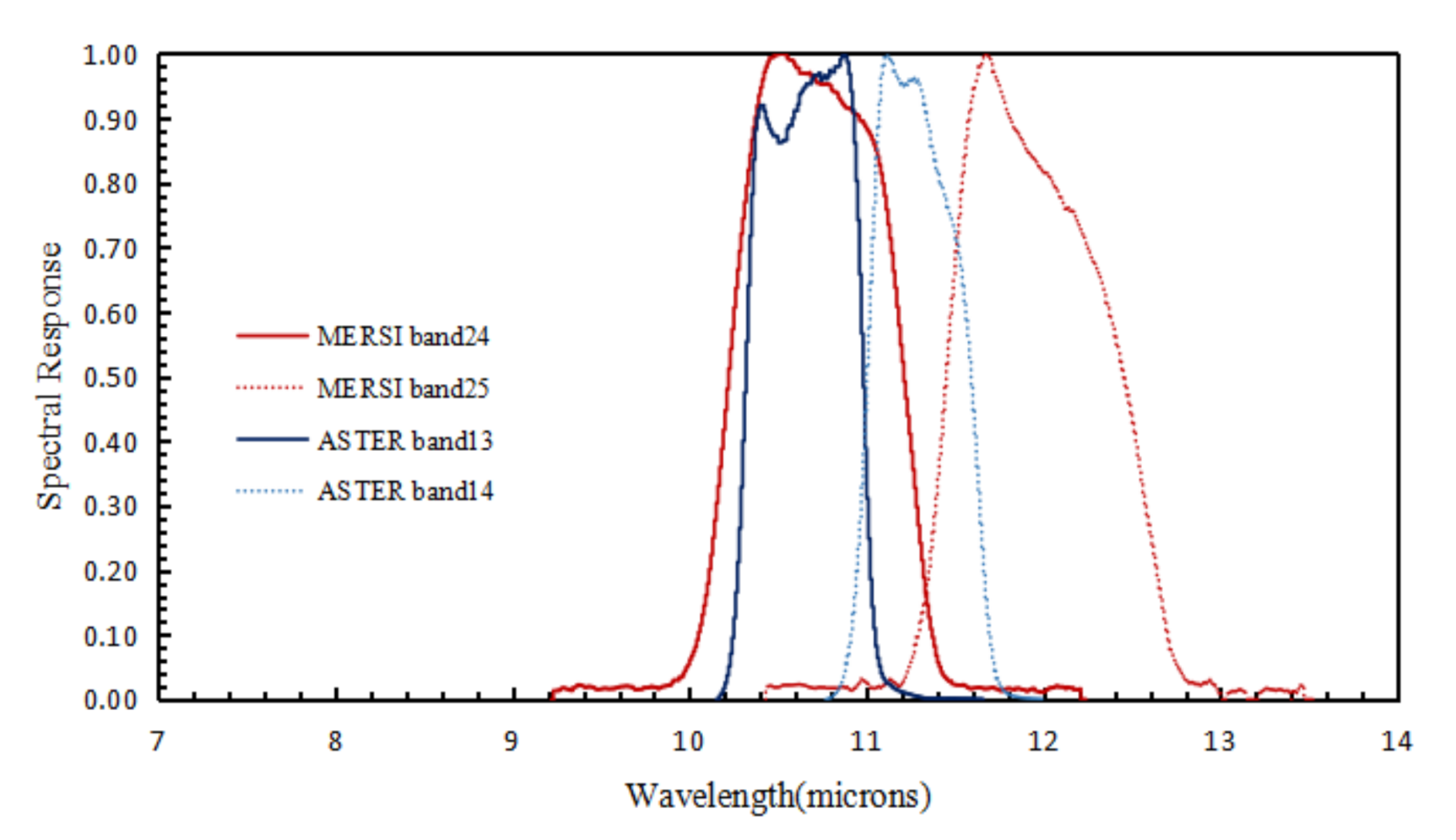
2.1. The FY-3D MERSI-II Data

The FY-3D MERSI-II data have a total of 25 bands, but in the study, only 9 bands (Table 1) for the required parameter estimation towards the LST retrieval were used. The TIR bands 24 (centered at 10.8 µm) and 25 (centered at 12.0 µm) were the key bands for LST retrieval. LST retrieval with TFSWA from the two TIR bands required the knowledge of both AT and LSE. Therefore, other bands were also necessary, so that the estimation of both AT and LSE could be conducted. Specifically, bands 3 and 4 were used for LSE estimation and bands 15, 16, 17, 18, and 19 were used for AT estimation. These bands are in different pixel sizes and all of them were resampled to 1000 m spatial resolution with the nearest neighbor resampling. Figure 1 gives the spectral response functions of FY-3D MERSI-II and ASTER TIR bands.

2.2. The TIGR Profile Database

The TIGR database [48,49] was a widely-used atmospheric profile database established by the French Weather Dynamics Laboratory for various atmospheric applications [50]. The TIGR database contains 2311 atmospheric profiles selected from global atmospheric samples from 1968 to 1989. Generally, the atmospheric profiles with a relative humidity greater than 90% or relative humidity between two successive layers greater than 85% can be regarded as cloudy profiles [49,50]. Thus, those profiles that meet the above-mentioned clear-sky conditions from the database were selected as the proposed clear-sky LST algorithm. Finally, 946 cloud-free profiles from the database were used, of which 236 ones belonged to the tropical atmosphere, 258 ones to the mid-latitude atmosphere, and 452 ones belonged to the polar atmosphere. The water vapor content of the cloud-free atmosphere profile varied from 0.06 to 6.27 g/cm2 and the atmospheric temperature at the ground layer ranged from 231 K to 314 K. They represent various atmospheric conditions at different seasons around the world.

2.3. The ASTER GED Dataset

The ASTER Global Emissivity Database (ASTER GED) [43], created by the National Aeronautics and Space Administration’s (NASA) Jet Propulsion Laboratory (JPL), California Institute of Technology, was used in the study for the LSE estimation. Eight parameters are available in the database, including the mean and standard deviation of global emissivity, land surface temperature, NDVI, and ancillary products containing land/water masks, latitude, longitude, and ASTER GDEM. Referring to ASTER data, the parameters for five ASTER TIR bands centering at 8.3 μm, 8.6 μm, 9.1 μm, 10.6 μm, and 11.3 μm are available. The dataset is distributed as 1° × 1° tiles at ~100 m and ~1 km spatial resolution in HDF5 and binary formats [24,43]. The data were generated using all cloud-free ASTER data from 2000 to 2008 with the TES algorithm [23] in conjunction with a water vapor scaling atmospheric correction method [51,52]. Validation over a set of global sites indicated an average band error of ~1% [52]. About 4% of pixels were found invalid probably due to incompletely expelling cloud contamination in high latitude regions [24,43].

2.4. The SURFRAD Measurements

Field measurements from four SURFRAD stations were applied in the study to evaluate the accuracy of the retrieved LST from FY-3D MERSI-II data. Established by the NOAA Office of Global Programs in 1993 to support satellite retrieval validation, modeling, climate, hydrology, and weather research for the United States [53], the SURFRAD network provides accurate, continuous, and long-term field measurements on the surface radiation budget every 1 min [54]. Seven stations are included and they are in a diverse climatological region ranging from the moist subtropical environment, the cool and dry northern plains to the hot and arid desert southwest, representing seven typical land cover types [54]. In this study, four SURFRAD stations, namely Bondvile (BND), Goodwin Creek (GWM), Penn State (PSU), and Sioux Fall (SXF), were selected for validation. Among them, the land cover type of the PSU station is crop, and the others are grass. Field LSTs were calculated from up-welling and down-welling long-wave radiation measurements of the SURFRAD stations through the Stefan-Boltzmann law as follows [55,56].
LST = F 1 ε b · F ε b · σ 1 / 4
where F and F are up-welling and down-welling thermal infrared (3–50 μm) irradiance in W·m−2 measured simultaneously at satellite overpass time, σ represents the Stefan-Boltzmann constant (5.670367 × 10⁻⁸ W·m−2·K−4), and εb refers to broadband long-wave surface emissivity estimated using the following equation [57].
εb = 0.197 + 0.025ε10 + 0.057ε11 + 0.237ε12 + 0.333ε13 + 0.146ε14
where ε10, ε11, ε12, ε13 and ε14 are the mean emissivity of ASTER GEDv3 bands 11, 12, 13, and 14, respectively.
It was found that the measured surface radiation of SURFRAD stations was generally greater than the actual one and the difference was 2–3 W·m−2 for crop and grass surface [58]. This difference might result in an error of −0.3–0.3 °C in LST estimation. Specifically, the LST estimation error during daytime was in −0.3–0 °C [58].

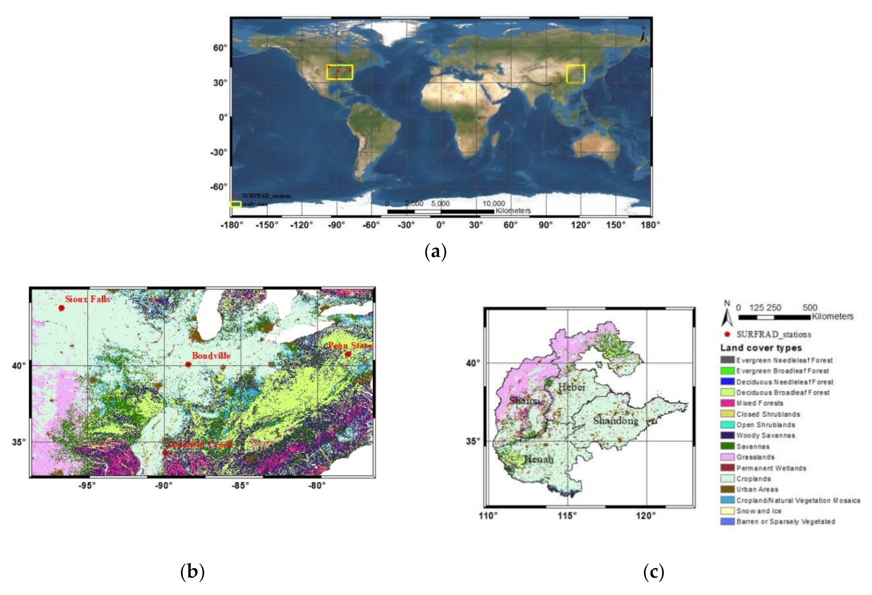
2.5. The Study Areas for Validation

Validation was necessary in this study. Two study areas are used to correspond two approaches of validation. The first validation was to use ground truth data from field measurements. Due to availability, we used the field measurements from 4 available SURFRAD stations in the USA to validate the improved TFSWA. Thus, for the validation, we needed to obtain FY-3D MERSI-II data covering the selected 4 SURFRAD stations in the USA and then compute the LST from the FY-3D MERSI-II data using the improved TFSWA. Comparison of the LST from field measurements with that from the retrieval would help us to understand the accuracy of the improved TFSWA for LST retrieval. The second approach of validation was cross-validation, i.e., to compare the retrieved LST from FY-3D MERSI-II data with the available satellite LST product. For this, we selected the MODIS LST product as a reference for the cross-validation. This is because the MODIS LST product has been widely applied to many studies and appreciated as one of the best satellite LST products in the world. Since FY-3D is a Chinese satellite for Earth observation, we selected Mid-East China as the region for the cross-validation with the MODIS LST product. The Mid-East China region has a latitude of 30°00′N to 45°00′N and longitude of 108°00′E to 123°00′E, including Henan, Shanxi, Hebei, and Shandong Province. Figure 2a shows the geographical location of the two study areas. Figure 2b gives the IGBP land cover types of the region in the USA and the four SURFRAD stations. Figure 2c shows the IGBP land cover types of the study area in China.

3. Methodology

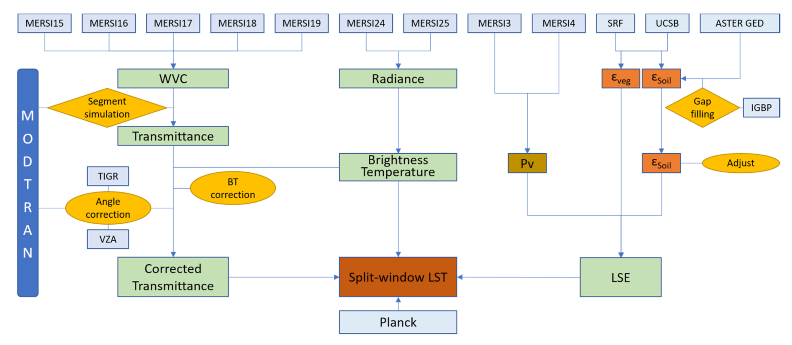
3.1. The Scheme for LST Retrieval

The scheme for LST retrieval is shown in Figure 3. Among three components, the left part is to estimate AT required in the LST retrieval, the right part is to estimate the LSE, and the central part is finally to retrieve LST. As shown in Figure 3, five FY-3D MERSI-II bands (15, 16, 17, 18, and 19) were used for the AT estimation, including the MODTRAN simulation, AWVC estimation, AT estimation, and the angle correction. Two FY-3D MERSI-II bands (3 and 4) were used in associated with the ASTER GED data to conduct the LSE estimation. In addition to these two essential parameters, the brightness temperatures of two TIR bands were also the required inputs for LST retrieval.

3.2. TFSWA for LST Retrieval

Qin et al. [22] developed a TFSWA for LST retrieval from NOAA-AVHRR bands 4 and 5, completely based on the mathematical derivation from the thermal radiance transfer equation. The TFSWA for FY-3D MERSI-II has the functions as follows:
Ts = A0 + A1T24 − A2T25
A0 = a24[D25(1 − C24 − D24)/(C24D25 − C25D24)] − a25[D24(1 − C25 − D25)/(C24D25 − C25D24)]
A1 = 1 + D24/(C24D25 − C25D24) + b24[D25(1 − C24 − D24)/(C24D25 − C25D24)]
A2 = D24/(C24D25 − C25D24) + b25[D24(1 − C25 − D25)/(C24D25 − C25D24)]
C24 = ε24τ24n
D24 = [1 − τ24n] [1 + (1 − ε24) τ24n]
C25 = ε25τ25n
D25 = [1 − τ25n] [1 + (1 − ε25) τ25n]
where Ts is the retrieved FY-3D MERSI-II LST (K); A0, A1 and A2 are the internal parameters; Ti is the brightness temperature (BT) of FY-3D MERSI-II TIR band i (i = 24 or 25) (K); τi is the AT for band i; εi is LSE for the band i; ai, and bi are the constants for the band i.
The constants for the two FY-3D MERSI-II TIR bands are determined as follows:
Li = Bi(T)/[∂Bi(T)/∂T] ≈ Bi(T)/{[Bi(T + ∆T) − Bi(T)]/∆T}
where Li is the derivative of the Planck function Bi(T) with temperature T for the FY-3D MERSI-II TIR band i, which could be approximated as [Bi(T + ∆T) − Bi(T))]/∆T for determination of the constants as follows.
Li = ai + biTi
where ai and bi are the constants for the band i. It assumes Li with T from −50 °C to 50 °C for the two FY-3D MERSI-II TIR bands and then the constants were determined finally as follows: a24 = −53.477, b24 = 0.3951, 24; a25 = −57.087, and b25 = 0.4292. With these constants, it is able to retrieve LST from the two FY-3D MERSI-II TIR bands under the conditions that the two required parameters AT and LSE are estimated. This algorithm is just for the cloud-free pixels’ LST estimation. Thus, the cloud detection product was used as the cloud mask layer to filter clear-sky pixels.

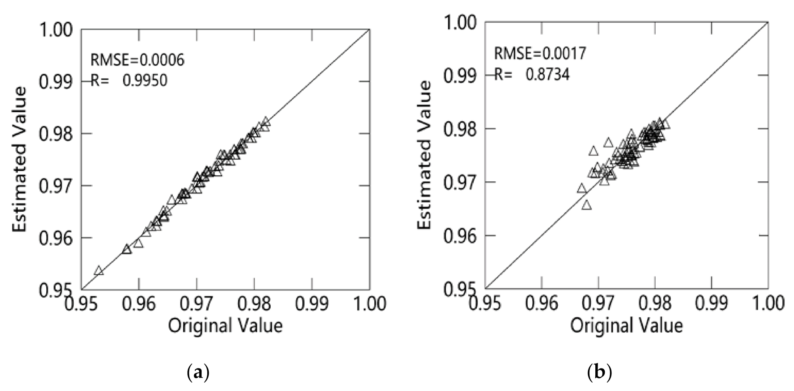
3.3. Estimation of AWVC

As seen in the previous section, AT is an essential parameter for LST retrieval with the improved TFSWA. AWVC is the most important factor affecting the variation of AT. Thus, the estimation of AT was generally converted from AWVC [4,13]. Three bands (bands 16, 17, and 18) of FY-3D MERSI-II were within the spectral range of atmospheric water vapor absorption (AWVA) so that it was able to estimate the WVC from these AWVA bands. It was found that the surface reflectance differed almost linearly with the wavelength for various ground surface types around the spectral range of AWVA [59,60]. Using this relationship, Kaufman et al. [60] proposed a ratio approach for the AWVC estimation for MODIS data. Following this approach, a similar method in the study was used to estimate AWVC.
Together with the other two non-absorption (TNA) bands (bands 15 and 19, close to the AWVA bands in spectral), the computation of the band ratio Ri for AWVC estimation is as follows:
R i = ρ i / ( ω i 1 ρ 15 + ω i 2 ρ 19 )
ω i 1 = λ 19 λ i λ 19 λ 15
ω i 2 = λ i λ 15 λ 19 λ 15
where Ri is the ratio of the AWVC band i to the TNA bands; ρ i is top-of-atmosphere (TOA) reflectance for the AWVC band i; ρ 15 and ρ 19 are TOA reflectance of the TNA bands 15 and 19, respectively; λi represents the central wavelength of the AWVA band i, which can be obtained in Table 1; ωi1 and ωi2 are the weight of the AWVC band i for TNA bands 19 and 15, respectively.
To establish this relationship, the atmospheric simulation program MODTRAN 5.2 was used in the study to simulate the TOA reflectance for the 3 AWVA bands with various atmospheric profiles having different AWVCs (0 g/cm2 to 7.5 g/cm2). To represent the actual situations in the real world, the atmospheric simulations for various conditions were performed, including different ground surface types (snow cover, forest, farm, desert, ocean, burnt grass, maple leaf, decayed grass, cloud deck, and old grass), rural aerosol model, 23 km visibility, and six standard atmospheres (US-1976, mid-latitude winter/summer, sub arctic winter/summer, and tropical atmosphere). Then, using the results from the simulation, a look-up table (LUT) showing the corresponding relationship between the ratio Ri and the AWVC was developed. This LUT or the regression functions (16)–(18) from this LUT were then used to estimate the AWVC (Wi) for each of the 3 AWVA bands.
W 16 = 0.0686   ln R 16 0.3126 2
W 17 = 0.0533   ln R 17 0.8779 2
W 18 = 0.0282   ln R 18 0.5968 2
Since the estimated AWVC for each of the 3 AWVA bands might be slightly different as a result of its spectral limitation in accurately reflecting the actual AWVC, a weighted average approach was developed in the study to determine the AWVC for the pixel as follows [59,60].
W* = f16W16 + f17W17 + f18W18
where W* is the estimated AWVC of the pixel; W16, W17, and W18 are the estimated AWVC of the pixel from the AWVA bands 16, 17, and 18, respectively, which were given by the LUT or the regression functions (16)–(18) after Ri of the AWVA band i was computed; f16, f17, and f18 are the weight coefficients of the 3 AWVA bands. The following functions (20)–(23) are used to calculate the coefficient fi:
fi = ηi/(η16 + η17 + η18)
η16 = |−0.0024*(W16)2 + 0.0260*W16 − 0.0976|
η17 = |−0.0081*(W17)2 + 0.0802*W17 − 0.2305|
η18 = |−0.0060*(W18)2 + 0.0606*W18 − 0.1862|
where ηi are computed numerically from simulated curves of transmittance versus AWVC as the sensitivity of the tranmittance (τi) to the AWVC (Wi) in each band i (16, 17, 18), which can be calculated from |∆τi/∆Wi|.
The estimated W* from Equation (19) is a combined two-way water vapor amount with effects of the optical path from viewing and sun-shining. For AT estimation, the vertical AWVC is needed. Based on the solar zenith angle (SZA) and the viewing zenith angle (VZA), the derived two-way water vapor amount W* is converted to the vertical column water vapor amount W using the following equation [59,60].
W = W*/[1/cos (VZA) + 1/cos (SZA)]
where W is the estimated AWVC of the pixel over the vertical column for AT estimation; VZA and SZA are the viewing zenith angle and solar zenith angle of the pixel, respectively.

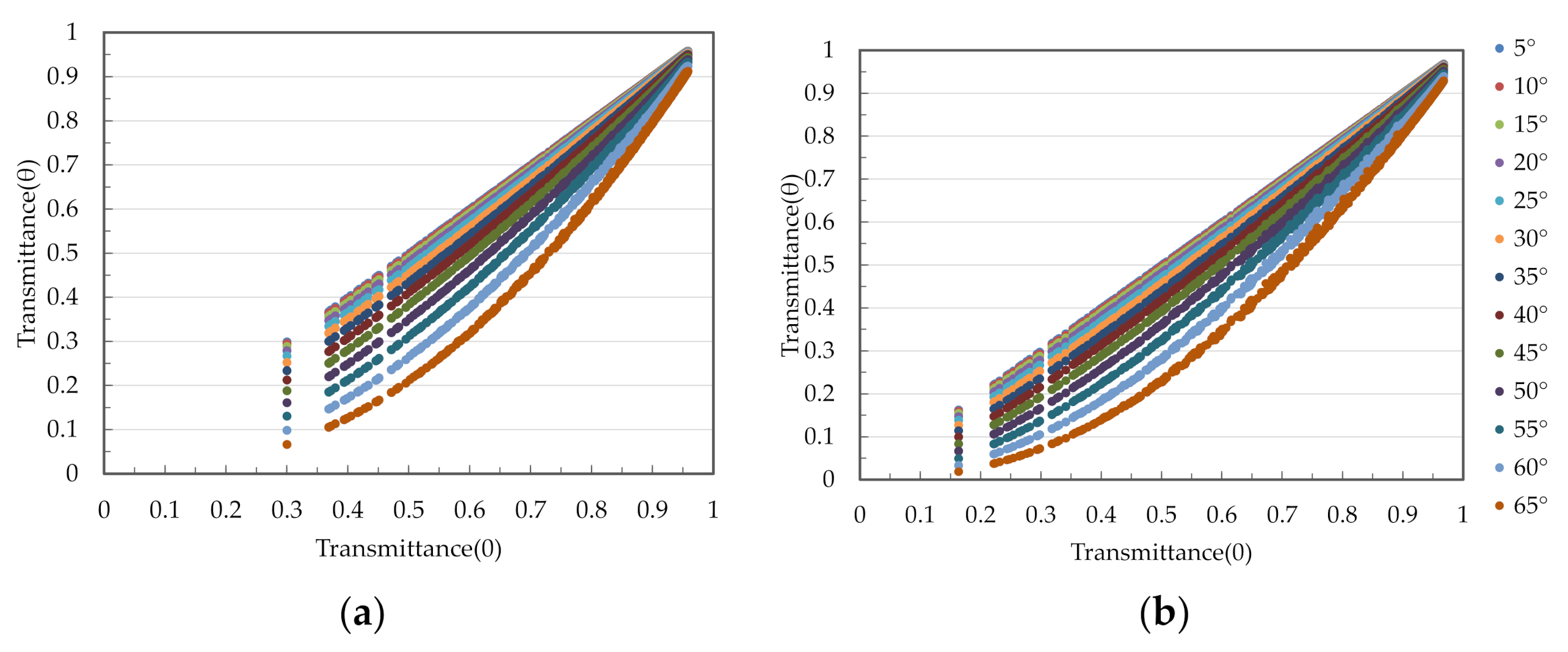
3.4. Estimation of AT

An AT estimation from AWVC is required to know the relationship between AT and AWVC [22,35,37]. To establish this relationship, MODTRAN 5.2 again was used to simulate the change of AT with AWVC for the two FY-3D MERSI-II TIR bands under various conditions including the atmospheric profiles, viewing angles, and surface types. Generally, AT decreases with AWVC under various atmospheric conditions. The simulation was performed for each of the six available standard atmospheres with AWVC changing from 0.1 g/cm2 to 7.0 g/cm2 for various viewing angles. Results of the simulation were used to construct an LUT for AT estimation from AWVC at the pixel level.
Due to the obvious VZA difference among the pixels, a two-step approach was established in the study for AT estimation. Firstly, τi(0), the AT at the nadir viewing with the AWVC (W) over the vertical column of the atmosphere for the two FY-3D MERSI-II bands 24 and 25, was estimated. This was done with the established LUT for AT estimation. The second step was to consider the effect of the pixel’s viewing zenith angle on AT. As is well-known, the pixels apart from the nadir had a VZA greater than 0 compared with the pixels at the nadir. This would increase the viewing path through the atmosphere. Consequently, the AT of the pixel would decrease [35]. The effect of VZA on AT had to be considered for the pixels apart from nadir. Assuming the AT with the VZA = 0 was demonstrated as τi(0) and the AT with VZA = θ was demonstrated as τi(θ) for the two FY-3D MERSI-II TIR bands, to minimize this angular effect, the atmospheric simulation using MODTRAN 5.2 to establish the relationship between τi(0) and τi(θ) was performed. Since the FY-3D data had a scanning swath of 2400 km, and the pixels at the far edge part might have had a VZA of ~55°, the simulation was conducted with the VZA varying from 0 to 65°. A total of 946 clear-sky atmospheric profiles from the TIGR database were used for the simulation. Figure 4 shows the results of the simulation for FY-3D MERSI-II TIR bands 24 and 25. The obvious difference as seen in Figure 4 was that the AT decreased remarkably with VZA. This was especially true when AWVC was very high or AT was quite low.
An angular correction model was established in the study to involve the effect of VZA on AT estimation as follows [35]:
τ i θ = a 1 i S 2 + a 2 i S + a 3 i τ i 2 0 + b 1 i S 2 + b 2 i S + b 3 i τ i 0 + c 1 i S 2 + c 2 i S + c 3 i
S =   sec θ 1
where a1i, a2i, a3i, b1i, b2i, b3i, c1i, c2i, and c3i are the coefficients of the angular correction models for band i, as shown in Table 2. Determination of the coefficients was done over the results from 26,656 simulations in MODTRAN 5.2 with 946 TIGR atmospheric profiles, six standard atmospheres, and 14 VZAs (the range is from 0° to 65°, the step is 5°). Table 2 clearly shows that correlation coefficients’ square R2 value were high up to 0.9999 and 1, implying that the fitting models are feasible for angular effect correction.

3.5. Estimation of LSE

Variation of LSE at the pixel scale is related to the surface types and their structures [39,61]. Under the condition that the LSE variations caused by internal reflection and distribution of natural surface [10,43,45] were not considered, LSE estimation could be done with a linear combination of the pixel’s components, mainly including soil and vegetation [39,41].
εi = εviPv + εsi(1 − Pv)
where εi is the emissivity for band i, εvi and εsi are the vegetation and bare soil components for band i, and Pv is the vegetation cover fraction calculated from NDVI [40]. Usually, such as spectral databases as the ASTER spectral dataset [62] and University of California at Santa Barbara (UCSB) emissivity library [63] were used to compute the εvi and εsi in Equation (27) for LSE estimation [39]. Moreover, the computed εvi and εsi from the databases were set as the same for all images. However, soil emissivity among different soil types may have great differences in magnitude. Consequently, this relatively wide range of emissivity variation among different soil types may cause significant effects on the accuracy of LST retrieval. To avoid these possible effects, an approach of estimating the soil emissivity from the ASTER GED product was proposed. The approach was composed of four steps: soil emissivity separation from ASTER GED product, IGBP based gap-filling for soil component emissivity, emissivity adjustment to FY-3D MERSI-II data, and the computation of LSE for the pixels of FY-3D MERSI-II data. Details are given as follows.

3.5.1. Estimation of Soil Emissivity from ASTER GED Product

ASTER GED product provides LSE for the entire land surface of the Earth. Viewing the grid of ASTER GED products as a mixture of vegetation and soil, it was able to separate the soil emissivity from the product. The separation can be done as follows [43]:
εsia = (εia − εvia Pva)/(1 − Pva)
Pva = [(NDVIa − NDVImin)/(NDVImax − NDVImin)]
where Pva is the vegetation cover fraction computed from ASTER GED mean NDVI data [64]; NDVImax and NDVImin are the maximum and minimum NDVI values in the ASTER GED product, which was obtained from 95% and 5% histogram intervals; εvia, εsia, and εia are the emissivity of vegetation component, bare soil component, and mean emissivity of the mixed grid for ASTER TIR band i, respectively. In the study, the emissivity of the vegetation component was computed as an average emissivity by convolving with the ASTER spectral response function (SRF) with vegetation emissivity spectrum from the ASTER spectral database [62] and UCSB spectral database [63]. The vegetation emissivity of 0.8981 for the ASTER TIR band 13 and 0.983 for band 14 were adopted in this study.

3.5.2. Gap Filling of ASTER Soil Emissivity

As mentioned previously in Section 2.3, the ASTER GED product includes some pixels (~4%) that involve invalid data, probably due to the effects of long-prone cloud cover [43,64]. These pixels with invalid data should be filled with proper data for LSE estimation. The MODIS land cover product (MCD12Q1) was used in the study to fill the gaps of LSE for the pixels with invalid data. Among the five schemes of the MODIS MCD12Q1 product, the International Geosphere Biosphere Program (IGBP) global vegetation classification was selected to determine the soil component emissivity of mixed pixels. The gap was filled according to the soil LSE look-up table (LUT) of the IGBP classes shown in Table 3 where soil types correspond to specific IGBP land surface types [45]. Furthermore, soil emissivity of ASTER TIR bands 13 and 14 were obtained from the spectral response functions (SRFs), the ASTER spectral database [62] and the UCSB emissivity [63]. Mean and standard deviation values were calculated for soil LSEs of ASTER TIR bands 13 and 14. It was found that the soil LSE ranges from 0.954 to 0.973 for different soil types. This relatively broad dynamic range of vegetation LSEs indicates that it is not reasonable to use the same soil emissivity for LSE for each pixel of FY-3D MERSI-II.

3.5.3. Adjustment of ASTER Soil Emissivity to FY-3D MERSI-II TIR Bands

Firstly, the emissivity for the target spectral bands of MRESI-II and ASTER were estimated with the UCSB and ASTER spectral databases. Then, the least-square fitting method was used to establish the conversion functions (Equations (30) and (31)) of bare soil emissivity, from the bare soil LSEs of ASTER channel 13 εs13a and channel 14 εs14a to those of MERSI-II bands 24 εs24m and 25 εs25m.
Figure 5 compares the estimated emissivity with the actual one computed from UCSB and ASTER spectral databases. The linear Pearson correlation coefficient R values for FY-3D MERSI-II TIR bands 24 and 25 were 0.9950 and 0.8734, respectively, and the RMSEs were 0.0006 and 0.0017, respectively. This excellent fitting performance indicates that the improved TFSWA could be used to estimate the bare soil emissivity for LST retrieval from the FY-3D MERSI-II data.
εs24m = 1.038 εs13a + 0.032 εs14a − 0.069
εs25m = −0.360 εs13a + 0.978 εs14a + 0.375

3.5.4. Calculation of the LSE for FY-3D MERSI-II

After the emissivity of bare soil εsim for FY-3D MERSI-II TIR bands 24 and 25 was calculated from the bare soil emissivity of ASTER TIR bands 13 εs13a and 14 εs14a, the land surface emissivity εim of each FY-3D MERSI-II pixel could be further estimated with the mixed pixel emissivity model, i.e., Equation (32), provided that FY-3D MERSI-II vegetation emissivity εvim and the corresponding vegetation cover fraction Pvm had been calculated from FY-3D MERSI-II NDVI data. The emissivity for FY-3D MERSI-II data can be calculated as follows:
εim = εvim Pvm + εsim (1 − Pvm)
where εim is the LSE of FY-3D MERSI-II data; εvim is the vegetation emissivity used to estimate the LSE for FY-3D MERSI-II TIR bands 24 and 25, which has the value as εv24m = 0.982 and εv25m = 0.984, respectively; εsim is the bare soil emissivity for LSE estimation. The FY-3D MERSI-II multi-year average bare soil emissivity (εsim) image could be obtained from the ASTER GED database’s mean emissivity to replace the bare soil emissivity constant usually used in the VCM method, which can reflect the variation of bare soil emissivity in space, thus improving the emissivity inversion accuracy.

3.6. Validation of the Improved TFSWA

Validation is necessary to evaluate the developed algorithm and to understand the possible errors caused by the major factors involved. Three methods were used in the study for the validation, including atmospheric radiation transfer (RTE) simulation by MODTRAN, T-based validation using SURFRAD field measurements, and cross-validation with the MODIS MYD11A1 product.

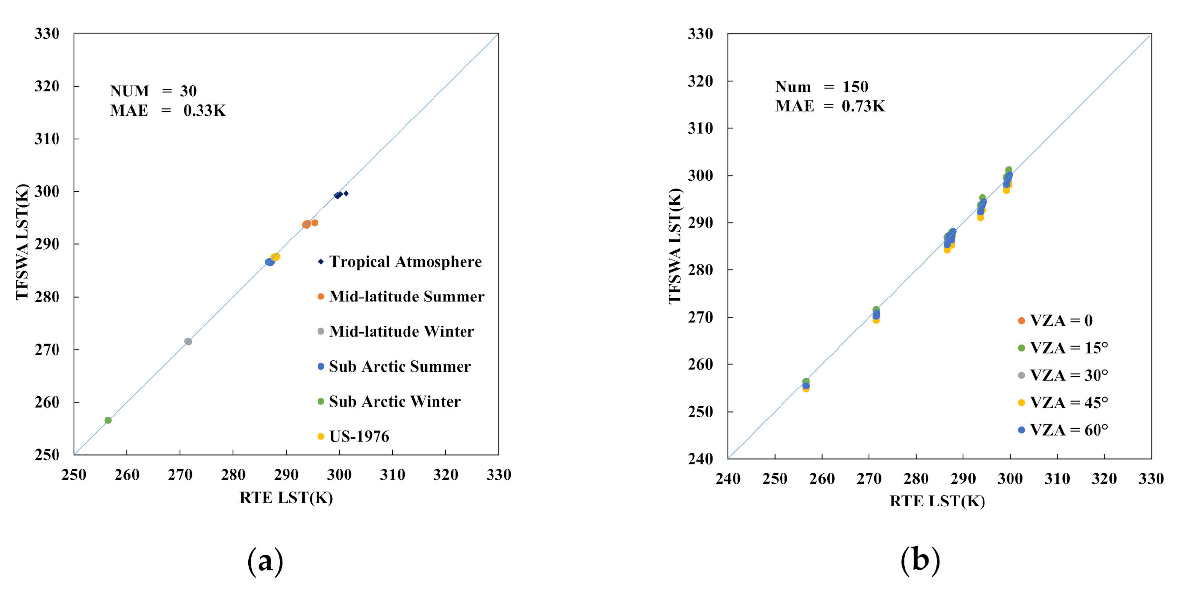
3.6.1. Validation with Atmospheric Radiation Transfer Simulation

Since the derivation of the TFSWA from the radiance transfer equation (RTE) was completed with several approximations to the relevant parameters of the equations, possible errors of the TFSWA were unavoidable as a result of these approximations. One way to understand this possible error was to compare the LST calculated from the atmospheric radiation transfer simulation and the retrieved MERSI-II LST by the TFSWA and the simulated dataset [65,66]. In the study, MODTRAN 5.2 was used to conduct this atmospheric radiation transfer simulation for the FY-3D MERSI-II TIR bands. The sensed TIR radiance of the FY-3D MERSI-II TIR band i could be computed as follows:
L i toa =   ε i B i T s τ i + 1 ε i τ i L i + L i
where Litoa, L, L and τi are the TOA radiance, up-welling radiance, down-welling radiance, and AT of the FY-3D MERSI-II TIR band i, respectively; Bi(Ts) is the Planck function to describe the emitted thermal radiance of ground as a blackbody with LST of Ts for the band i; εi is the LSE of the band i. The value of all these parameters for the specific conditions (such as AWVC and LST) used for the simulation could be obtained from the output of the simulation with the MODTRAN 5.2 program. The simulation was conducted with the LSE = 0.978 for band 24 and 0.983 for band 25 of FY-3D MERSI-II. The emissivities used here were calculated from the UCSB emissivity dataset and ASTER spectral library, which can represent mixed land types according to the actual estimated emissivity values using the MERSI-II LSE algorithm. Therefore, RTE LST (Ts) used for validation can be obtained from the inverse Planck function derived from Equation (33).
Since the altitude of the FY-3D satellite was 750 km, which was much higher than the TOA height, the converted brightness temperature (BT) from Litoa with Planck function could be viewed as the corresponding at-sensor brightness temperature for FY-3D MERSI-II TIR bands 24 and 25. Accordingly, the corresponding FY-3D MERSI-II LST could then be retrieved from the brightness temperature with the improved TFSWA in combination with the assumed LSE used for the simulation and the simulated AT (τi).
The simulation was performed with six standard atmospheric models for five water vapor contents (0.5–4.5, step = 1, unit: g/cm2) and five VZAs (0°~60°, step = 15°).

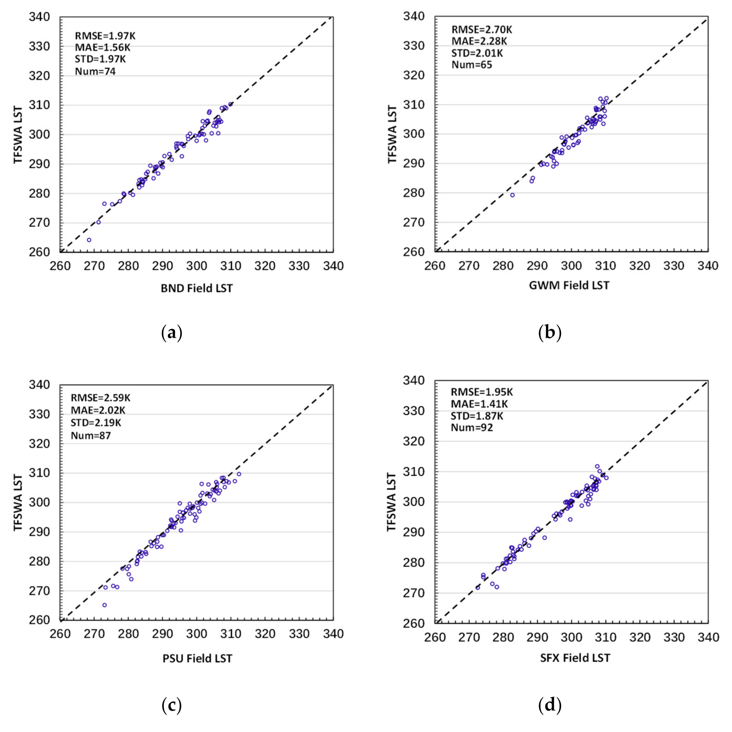
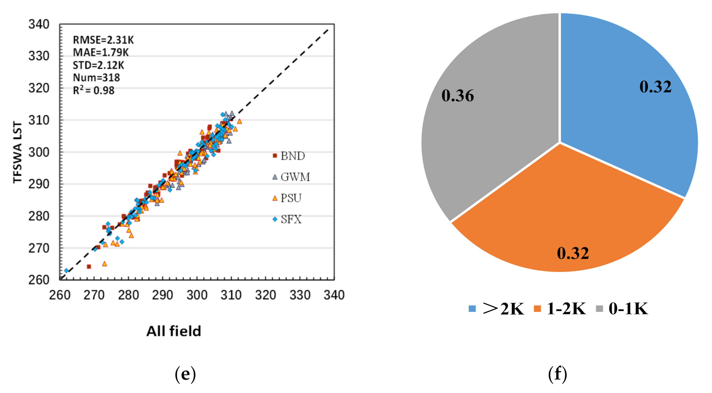
3.6.2. Validation with Field Measurements

In the study, field measurements from the available four stations in the central USA (Figure 2b) were obtained from SURFRAD websites to validate the accuracy of the improved TFSWA. Land cover types of the four stations mainly included cropland (PSU) and grassland (BND, GWM, and SXF). The whole-year field measurement datasets of each station in 2020 were downloaded and the FY-3D MERSI-II LST of the region covering the four stations were retrieved. Using the latitude and longitude of the four stations, the pixel values were extracted from the retrieved FY-3D MERSI-II LST of each station from all the clear-sky scenes in 2020 for the validation. A total of 318 clear-sky FY-3D MERSI-II LST samples were used covering the whole year of 2020. Then, the field measurements of the LST of each station at the time closest to FY-3D MERSI-II overpass time were obtained and used to compare with the retrieved FY-3D MERSI-II LST. It was assumed that the field measurements of LST were the true LST of the station at the FY-3D MERSI-II overpass time. Despite the incompatibility between the field measurements of LST as a point and the FY-3D MERSI-II LST as a measurement from a pixel with a size of 1000 m × 1000 m, which is far from the point measurement of each station, the comparison of the difference between the retrieved LST and the measured LST still provides some general information about the accuracy of the TFSWA for LST retrieval from the FY-3D MERSI-II data in the real world. The field measurement of LST was calculated with Equation (1) given in Section 2.4.

3.6.3. Cross-Validation with MODIS LST Products

The MODIS LST product MYD11A1 has been widely used for various applications. Since the overpass time of the FY-3D satellite is close to that of MODIS, a comparison of the retrieved FY-3D MERSI-II LST with the MYD11A1 LST can also provide useful information about the accuracy of the TFSWA for LST retrieval from the FY-3D MERSI-II data. Different seasons and land surface types were considered for the comparison. The daytime FY-3D MERSI-II data in 2020 in Mid-East China were obtained for LST retrieval with the TFSWA. The daily MODIS LST products in 2020 in the same region of Mid-East China were collected for comparison.
Generally, cross-validation is done over single-day images from two sources. In our study, we computed the FY-3D MERSI-II LST for each day of the entire year 2020 and downloaded the daily MODIS LST product covering the same Mid-East China region for the same year. The retrieval of the LST from satellite images was only possible for the clear-sky condition when thermal infrared radiance could transfer from the ground through the atmosphere to the sensor at space for remote sensing of LST. Therefore, our daily cross-validation was completed for only the clear-sky pixels.
In addition to the accuracy analysis of single-day LST data, the monthly average LST between MERSI-II LST and MODIS LST (LSTMERSI-II − LSTMODIS) were also further calculated and analyzed in the study. This is because the monthly average LST can provide some more information about the general trend of spatial variation of the LST over the same region in comparison to the single-day LST image. Thus, cross-validation with the monthly average LST between the two LST datasets was also necessary. Since there was less cloud contamination in July 2020, the monthly average LST results of MERSI-II and MODIS for Mid-East China (Figure 2c) in this month were calculated.
In this study, for evaluating the difference of FY-3D LST and MODIS LST in different seasons of the year, MERSI-II and MODIS LSTs in January, April, July, and October 2020 were selected to represent the four seasons of the year, respectively. In addition, a series of conditions for observation time and angle to select proper points was used, to ensure that the pixel pairs selected from the two kinds of datasets had the most similar observation conditions. The local solar time is used for the observing time of the two LST datasets, and the clear-sky pixels in the two LST datasets with a time gap within 5 min were applied [67,68,69]; based on these selected pixels of two datasets, pixels with the difference between the tangent ratio of the view zenith angle less than 0.01 were regarded as having a similar atmospheric optical path [68,70,71,72].

4. Results and Analysis

4.1. Results from Validation with Atmospheric Radiation Transfer Simulation

Figure 6a shows the scatter plots of the simulated RTE LST from MODTRAN and the retrieved LST with the improved TFSWA for VZA = 0, which have 30 samples (six atmospheric models, five water vapor contents, and VZA = 0). In addition, Figure 6b shows the scatter plots for the entire five VZAs, which have 150 samples (six atmospheric models, five water vapor contents, and five VZAs). Since the LST in different atmospheric models has a great difference, for example, 256.58 K in the sub-Arctic winter atmosphere and 299.20 K in the tropical atmosphere, scatter plots of the samples shown in Figure 6 are not evenly distributed but in a cluster for each atmospheric condition. All the sample dots in both Figure 6a,b are distributed around the 1:1 line, indicating that the retrieved LSTs with the TFSWA are very close to the RTE LSTs in all cases for the six atmospheric models. Despite this very good closeness between the simulated RTE LST and TFSWA LST for the six atmospheric conditions, slight differences between them still exist for different VZAs for a specific atmosphere condition. The statistical result of the difference indicates that ~70% of the difference ΔTs are within 1 K. The mean average value (MAE) shown in Figure 6a for 30 samples of VZA = 0 is 0.33 K, while the MAE in Figure 6b for a total of 150 samples of five VZAs is 0.73 K. These statistical results prove that the improved TFSWA is very good for LST retrieval from FY-3D MERSI-II data.

4.2. Results from Validation with Field Measurements

Figure 7 presents the validation results with the field measurement LST datasets. Scatter plots of the field measurement LST with the retrieved LST are shown in Figure 7a for Bondville station. Though the RMSE in the Bondville station is 1.97 K, most points in Figure 7a are on the non-bias line, implying the high accuracy between the retrieval LST and the field measurement LST. A similar situation is also seen in Figure 7b for Goodwin Creek station even though the retrieved LST is slightly underestimated for the field measurement LST and the RMSE increases to 2.70 K. This is probably due to the mismatch of the station in spatial location over the FY-3D MERSI-II images. Another reason may be the relatively spatial heterogeneous ground surface around the station. Relatively high RMSE is also observed in Figure 7c for PSU station where ground heterogeneity is high. Figure 7d shows a better RMSE (1.95 K) than those of Figure 7a–c. The scatter plots of all the sample points for the four stations are given in Figure 7e. Figure 7f presents the statistics of the LST difference for each station. According to the statistical analysis in Figure 7f, about 113 samples (36%) have an LST difference within 1 K. Another 103 samples (32%) are within 1–2 K. The rest of the 102 samples (32%) are with an LST difference greater than 2 K. The MAE of the four stations changes from 1.41 K (SFX) to 2.28 K (GWM). RMSE, MAE, and R2 of all samples for the four stations shown in Figure 7e are 2.31 K, 1.79 K, and 0.98, respectively. This indicates there is very good consistency between the retrieved LST and the field measurement LST even though they are not completely matched in spatial size.

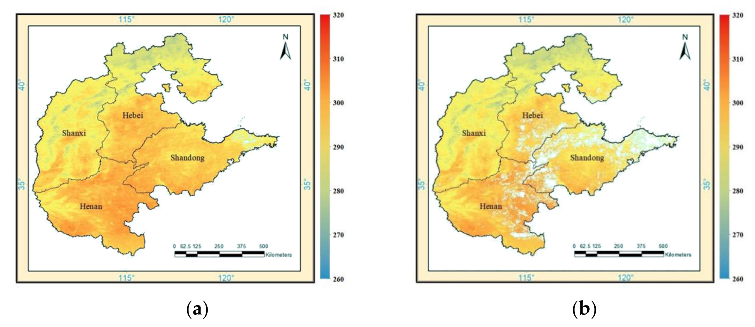
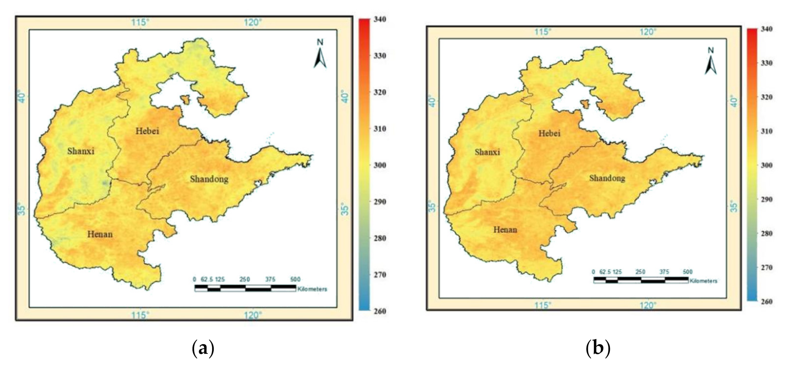
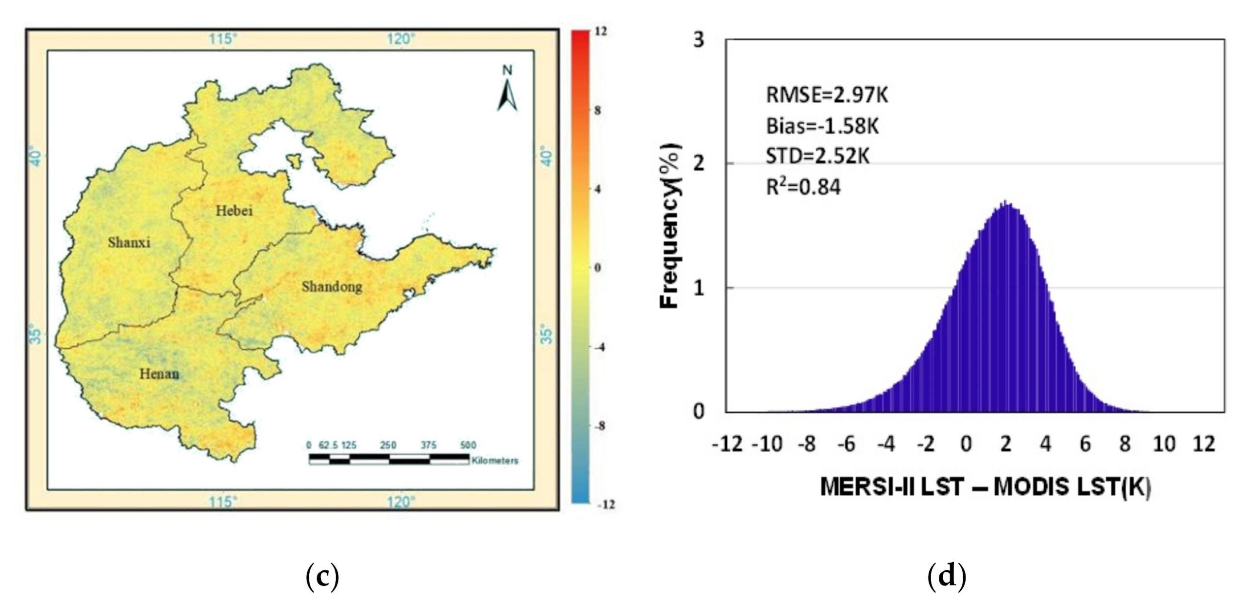
4.3. Cross-Validation on Daily and Monthly Average Images

Figure 8 compares the FY-3D MERSI-II LST and MODIS LST on 22 October 2020 over Mid-East China, which includes Shanxi, Hebei, Shandong, and Henan provinces of China. The overpass time of FY-3D MERSI-II on October 22 was about 13:30 h (local solar time) over this region, while the transit time of MODIS on this day was also about 13:30 h, indicating they were comparable for the LST variation. According to the statistical analysis, LSTs in the study area range from 268.6 K to 309.30 K. In addition, from Northwest to Southeast, the LSTs increase evidently. The LSTs in the Southeast near the ocean are higher, mainly above 290 K. In comparison, those in Northwest China are mostly less than 290 K. Some relatively lower LSTs below 273.15 K are mainly distributed in Shanxi and Hebei province where Taihang Mountain, Lvliang Mountain, and Yanshan Mountain are located. Furthermore, there is quite a similar trend in the MERSI-II and MODIS LST images. In addition, as shown in Figure 8c, we analyze the difference (LSTMERSI-II − LSTMODIS) between the two LST maps. According to the statistical analysis, for the LST difference LST image in Figure 8c, the RMSE, bias, STD, and R2 are 1.74 K, 0.92 K, 1.47 K, and 0.96, respectively. For the frequency histogram graph shown in Figure 8d, the LST difference follows the normal distribution. In Figure 8, some pixels with invalid data result from cloud contamination distributed in both LST images. Because of the different transit times of the two sensors, the spatial distribution of invalid data in the two images are not the same for different cloud coverage.
Figure 9 shows the monthly average LST of FY-3D MERSI-II (a), MODIS (b), the LST difference between them (c), and the frequency histogram of LST difference (d). As shown in Figure 9a,b, the LST distribution in the MERSI-II and MODIS monthly average LST is highly consistent in the spatial distribution, and the difference also follows the normal distribution in Figure 9d. For the LST difference distribution in Figure 9a,b, relatively low LSTs are mainly distributed in Northern Hebei, Shanxi, and Eastern Henan where the mountains are located. In the meantime, it can be seen from the LST difference image in Figure 9c that the negative LST difference value mainly appears in the same location. According to the statistic result, for the difference of the monthly average LST in July 2020, the RMSE, bias, R2, and STD are 2.97 K, −1.58 K, 0.84, and 2.52 K, respectively.
Figure 10 shows the scatter plots between MERSI-II and MODIS LST in January, April, July, and October 2020. According to the statistical analysis in Figure 10, there are significant differences in LST for different seasons. The R2 range from 0.84 (July) to 0.96 (January); the RMSE (2.52 K), MAE (1.96 K), and standard deviation (2.46 K) are relatively large in July, while in January, the RMSE (1.57 K), MAE (1.21 K) and standard deviation (1.57 K) are relatively low.

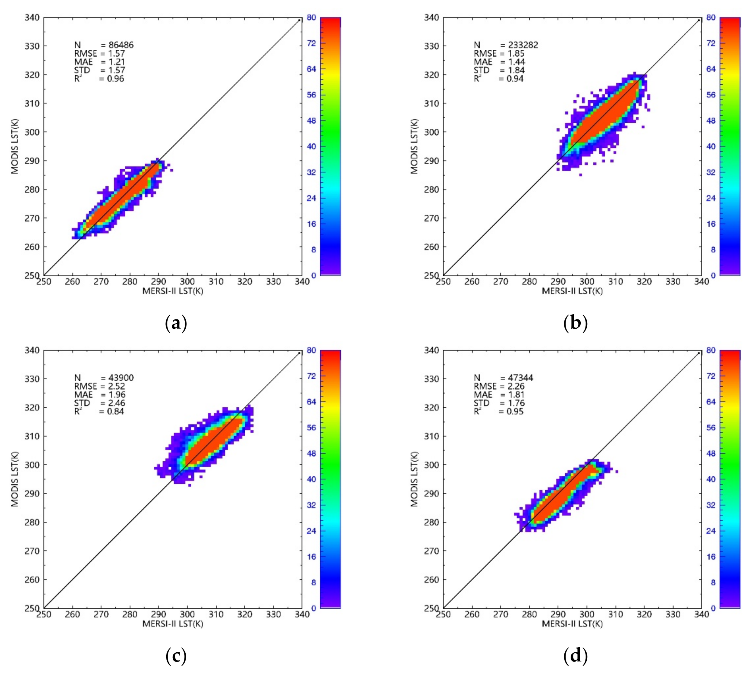
4.4. Cross-Validation over Different Land Surface Types

To clarify the different land cover types of MERSI-II, the variation of surface temperature accuracy of FY-3D MERSI-II with different types of surface coverage is analyzed. There are four types of land cover in the study area: deciduous broad-leaved forest (DBF), woody grassland (WS), grassland (GL), and farmland (CL). Figure 11 shows the correlation coefficient (R2), root mean squared error (RMSE), mean absolute error (MAE), standard deviation (STD), and other precision evaluation indexes of FY-3D MERSI-II LST over different land cover types in the summer of 2020 (June to August). Figure 11 shows the scatter plots of FY-3D MERSI-II and MODIS LST in the summer of 2020 (June to August). According to the chart, the land cover type has a significant impact on LST. The correlation coefficients of the four types of land cover are all relatively high, from 0.93 of the woody grassland to 0.98 of the other land cover types. In addition, the RMSE (1.98 K) and STD (1.85 K) of deciduous broad-leaved forests are the smallest, while the RMSE (2.87 K) and STD (2.87 K) of woody grasslands are the largest. In addition, the deciduous broadleaf forest has a minor MAE (1.46 K) and a more significant correlation coefficient (0.98), while the woody grassland has a more significant MAE (1.74 K) and the smallest correlation coefficient (0.93).

5. Discussion

The accuracy of the TFSWA algorithm is mainly influenced by the AWVC, transmittance, and LSE. The BT, LSE, and transmittance changed with different VZAs, for the pixels with extreme VZA that will induce more error. In the research, transmittance angular correction was performed carefully to minimize part of the angle effects in MERSI-II LST retrieval. Some additional factors should also not be neglected. Some errors were induced in the validation using ground data. As described above, the error for the SURFRAD crop and grass sites during daytime was about −0.3–0 °C [58]. This is another non-negligible error source for validation. Cloud detection errors inevitably exist in the cloud mask layer, especially when thin clouds exist. Moreover, some pixels with lousy quality and strips are inside in MERSI-II data. In this study, all test points for in-situ validation were checked carefully to exclude undetected clouds or bad-quality pixels to minimize the effect of cloud contamination and image quality in the validation work. In addition, a series of potential relating factors that may lead to LST errors, such as soil water content, surface air, humidity, wind speed, air temperature, should be analyzed in the near future [32].
To validate the accuracy and adaptability of the TFSWA algorithm, the MERSI-II LST with MYD11A1 LST for different seasons and land surface types were compared. According to the single-day and single-month LST comparison in Section 4.3, the LST difference along with mountains was more significant. This may be because the spatial-temporal variation of surface humidity in the rugged areas caused more uncertainty of cross-validation results. [68,71,72] As described in the monthly cross-validation, one can find that the LSTs in July had relatively low accuracy, the maximum standard deviation (2.46 K) existed in July and the minimum one (1.57 K) is in January. These results are mainly consistent with the previous studies [68,70,72]. This result may be due to the considerable spatial variation of LST because the difference of LST between bare soil and vegetation is more significant in July [72]. The influence of land surface emissivity may cause the difference. Moreover, the error of LSE may lead to more considerable differences between the two LST data sources in July. Another reason for the significant standard deviation of July LST may be the increasing influence of atmospheric change. The monsoon climate in Central and Eastern Asia is warm and humid, and the atmospheric water vapor content increases, which leads to the increase of LST error to a certain extent.
For the cross-validation results of various land cover types, the LST accuracy of the deciduous broad-leaved forest was relatively high than that of other land surface types, while the accuracy of woody grassland was the lowest. The reason for these results is mainly that the spatial structure of the evergreen broad-leaved forest is relatively uniform. At the same time, the woody grassland usually has more significant spatial heterogeneity, and the LSTs observed are easily affected by observation and illumination conditions [72]. Therefore, for land cover types with substantial spatial homogeneity, such as evergreen broad-leaved forest and grassland, the difference of LST retrieved from the two sensors is relatively small. In contrast, for rugged land surfaces, especially for poor or sparse vegetation land cover, the difference is relatively considerable. Besides, about three pixels of geometric positioning difference can be found between the MODIS and FY-3D MERSI-II data; the geographical position error is another influencing factor that should not be negligible for cross-validation at the 1000 m scale.
A limitation of this LST estimation scheme that should be noticed is that, the transmittance estimation models were simulated according to the standard atmospheric models inside MODTRAN, which was decided by the latitude and observing date of the image. For example, for the LST retrieval in the USA, the 1976 USA atmospheric model was used. However, for the global LST estimation, how to properly use these standard atmospheric models is an issue to address. In the next step, we plan to explore transmittance models that can be used for global LST estimation from numerous representative profiles. In addition, in the process of LSE estimation shown in Section 3.5, we calculated the NDVImax and NDVImin values using 95% and 5% percentiles for 1 km × 1 km tiles, while for different tiles of ASTER GED datasets, the NDVImax and NDVImin values are different. This could lead to some strips in the mosaic edges of ASTER GED soil emissivity tiles, which will result in some uncertainties in the process of LSE estimation. In the meantime, to derive soil emissivities with Equations (28) and (29), we applied average vegetation emissivities from ASTER and USCB databases in channels ASTER 13 and ASTER 14. Thus, the unique calculated values can have a significant impact on the soil emissivities. Although the dynamic range of vegetation specific emissivity is relatively small compared with soil specific emissivity, the soil specific emissivity can be underestimated or overestimated in certain areas where the vegetation specific emissivity is higher or lower than the average. In the near future, it should also be considered to develop an algorithm to obtain the vegetation emissivity distribution map to substitute the average values to further minimize the influence of mean vegetation LSE.

6. Conclusions

FY-3D MERSI-II, the second generation of the Chinese meteorological satellite for Earth observation, has two TIR bands for LST retrieval, and hence may have great potential for many environmental applications such as agricultural drought monitoring. In this study, an improved TFSWA has been developed for LST retrieval from FY-3D MERSI-II data. Essential coefficients of the TFSWA were carefully and precisely estimated according to the spectral features of the FY-3D MERSI-II TIR bands for LST retrieval. The ASTER GED and IGBP products were used to estimate the key parameter LSE required for LST retrieval with the improved TFSWA. The AT estimation equations and band ratio LUT for AWVC estimation were established based on the simulation database obtained from MODTRAN 5.2 and TIGR atmospheric profiles. The swath of FY-3D MERSI-II data is ~2400 km, which may significantly increase the optical path of the pixels apart from the nadir and such an increase in optical path may perform an obvious effect on the magnitude of AT for TIR remote sensing. A viewing zenith angle (VZA) correction equation was proposed in the study to consider this effect on AT estimation for precise LST retrieval from the FY-3D MERSI-II data.
Validation is very necessary for the improved TFSWA developed in the study. Three approaches were adopted to assess the applicability of the improved TFSWA: simulated RTE LSTs, field data, and MODIS LSTs. Compared with the RTE LSTs simulated by MODTRAN 5.2, the improved TFSWA had an LST estimation error MAE of <1 K, implying the applicability of the improved TFSWA for LST retrieval from the FY-3D MERSI-II data. Validation with 318 field samples from the available four stations of the SURFRAD network indicated that the average MAE and R2 of the scenes at the four stations were about 1.79 K and 0.98. Therefore, it could be concluded that the improved TFSWA developed in the study can be a good algorithm for LST retrieval from FY-3D MERSI-II data with acceptable accuracy. Cross-validation with MODIS LST products MYD11A1 was also completed over the Mid-East China region for different land surface types and seasons. Results from the cross-validation showed that the LST accuracy varied considerably in different seasons and over various land cover types. According to the statistical analysis, the land cover type had a significant impact on LST. The LST accuracy of the deciduous broad-leaved forest was relatively higher than that of other land surface types, while the accuracy of woody grassland was the lowest. For the cross-validation results of monthly average LSTs, the standard deviation values range from 1.57 K (in January) to 2.46 K (in July). Correlation coefficients between FY-3D MERSI-II LST and MODIS LST over the Mid-East China region were high up to 0.84~0.98 in different seasons and land cover types, implying that the MERSI-II LST generally had a high consistency with the MYD11 LST. The high consistency proves that the improved TFSWA has an acceptable accuracy for LST inversion of FY-3D MERSI-II data.

Author Contributions

W.D. and Z.Q. wrote the manuscript and worked on the methodology. J.F. collected and preprocessed the FY-3D MERSI-II data. C.Z., Q.H. and K.C. participated in the processing of LSE, the ground measurements, and the cross-validation. K.C. and B.A. gave support on TIGR data processing. Z.Q., J.F. and Q.H. provided suggestions for the correction of the final manuscript. All authors have read and agreed to the published version of the manuscript.

Funding

This study was supported by the National Key Research and Development Program of China (Grant No.: 2019YFE0127600, 2016YFA0600302) and the National Natural Science Foundation of China (Grant No.: 41771406, 41921001).

Acknowledgments

We sincerely thank Maofang Gao and Sibo Duan from Chinese Academy of Agricultural Sciences for their assistance in water vapor retrieval and TIGR data processing in the study.

Conflicts of Interest

The authors declare no conflict of interest.

References

  1. Ma, X.; Jin, J.; Zhu, L.; Liu, J. Evaluating and improving simulations of diurnal variation in land surface temperature with the Community Land Model for the Tibetan Plateau. PeerJ 2021, 9, e11040. [Google Scholar] [CrossRef]
  2. Fan, X.; Tang, B.-H.; Wu, H.; Yan, G.; Li, Z.-L. Daytime Land Surface Temperature Extraction from MODIS Thermal Infrared Data under Cirrus Clouds. Sensors 2015, 15, 9942–9961. [Google Scholar] [CrossRef] [PubMed] [Green Version]
  3. Qin, Z.; Berliner, P.; Karnieli, A. Ground temperature measurement and emissivity determination to understand the thermal anomaly and its significance on the development of an arid environmental ecosystem in the sand dunes across the Israel–Egypt border. J. Arid Environ. 2005, 60, 27–52. [Google Scholar] [CrossRef]
  4. Qin, Z.; Karnieli, A.; Berliner, P. Remote sensing analysis of the land surface temperature anomaly in the sand-dune region across the Israel-Egypt border. Int. J. Remote Sens. 2002, 23, 3991–4018. [Google Scholar] [CrossRef]
  5. Leng, P.; Song, X.; Duan, S.-B.; Li, Z.-L. A practical algorithm for estimating surface soil moisture using combined optical and thermal infrared data. Int. J. Appl. Earth Obs. Geoinf. 2016, 52, 338–348. [Google Scholar] [CrossRef]
  6. Anderson, M.C.; Hain, C.R.; Wardlow, B.; Pimstein, A.; Mecikalski, J.R.; Kustas, W.P. Evaluation of Drought Indices Based on Thermal Remote Sensing of Evapotranspiration over the Continental United States. J. Clim. 2011, 24, 2025–2044. [Google Scholar] [CrossRef]
  7. Eleftheriou, D.; Kiachidis, K.; Kalmintzis, G.; Kalea, A.; Bantasis, C.; Koumadoraki, P.; Spathara, M.E.; Tsolaki, A.; Tzampazidou, M.I.; Gemitzi, A. Determination of annual and seasonal daytime and nighttime trends of MODIS LST over Greece—climate change implications. Sci. Total Environ. 2018, 616–617, 937–947. [Google Scholar] [CrossRef]
  8. Zhang, F.; Kung, H.; Johnson, V.C.; LaGrone, B.I.; Wang, J. Change Detection of Land Surface Temperature (LST) and some Related Parameters Using Landsat Image: A Case Study of the Ebinur Lake Watershed, Xinjiang, China. Wetlands 2017, 38, 65–80. [Google Scholar] [CrossRef]
  9. Hao, Z.; Yuan, X.; Xia, Y.; Hao, F.; Singh, V.P. An Overview of Drought Monitoring and Prediction Systems at Regional and Global Scales. Bull. Am. Meteorol. Soc. 2017, 98, 1879–1896. [Google Scholar] [CrossRef]
  10. Duan, S.-B.; Li, Z.-L.; Wang, C.; Zhang, S.; Tang, B.-H.; Leng, P.; Gao, M.-F. Land-surface temperature retrieval from Landsat 8 single-channel thermal infrared data in combination with NCEP reanalysis data and ASTER GED product. Int. J. Remote Sens. 2018, 40, 1763–1778. [Google Scholar] [CrossRef]
  11. Jiménez-Muñoz, J.C.; Cristóbal, J.; Sobrino, J.A.; Soria, G.; Ninyerola, M.; Pons, X. Revision of the Single-Channel Algorithm for Land Surface Temperature Retrieval from Landsat Thermal-Infrared Data. IEEE Trans. Geosci. Remote Sens. 2009, 47, 339–349. [Google Scholar] [CrossRef]
  12. Tang, B.-H.; Shao, K.; Li, Z.-L.; Wu, H.; Nerry, F.; Zhou, G. Estimation and Validation of Land Surface Temperatures from Chinese Second-Generation Polar-Orbit FY-3A VIRR Data. Remote Sens. 2015, 7, 3250–3273. [Google Scholar] [CrossRef] [Green Version]
  13. Li, Z.-L.; Tang, B.-H.; Wu, H.; Ren, H.; Yan, G.; Wan, Z.; Trigo, I.F.; Sobrino, J.A. Satellite-derived land surface temperature: Current status and perspectives. Remote Sens. Environ. 2013, 131, 14–37. [Google Scholar] [CrossRef] [Green Version]
  14. Dash, P.; Göttsche, F.-M.; Olesen, F.-S.; Fischer, H. Land surface temperature and emissivity estimation from passive sensor data: Theory and practice-current trends. Int. J. Remote Sens. 2002, 23, 2563–2594. [Google Scholar] [CrossRef]
  15. Prata, A.J.; Caselles, V.; Coll, C.; Sobrino, J.A.; Ottle, C. Thermal remote sensing of land surface temperature from satellites: Current status and future prospects. Remote Sens. Rev. 1995, 12, 175–224. [Google Scholar] [CrossRef]
  16. Jiménez-Muñoz, J.C.; Sobrino, J.A. A generalized single-channel method for retrieving land surface temperature from remote sensing data. J. Geophys. Res. Space Phys. 2003, 108. [Google Scholar] [CrossRef] [Green Version]
  17. Cristóbal, J.; Jiménez-Muñoz, J.C.; Sobrino, J.A.; Ninyerola, M.; Pons, X. Improvements in land surface temperature retrieval from the Landsat series thermal band using water vapor and air temperature. J. Geophys. Res. Space Phys. 2009, 114. [Google Scholar] [CrossRef]
  18. Qin, Z.; Karnieli, A.; Berliner, P. A mono-window algorithm for retrieving land surface temperature from Landsat TM data and its application to the Israel-Egypt border region. Int. J. Remote Sens. 2001, 22, 3719–3746. [Google Scholar] [CrossRef]
  19. Coll, C.; Caselles, V. A split-window algorithm for land surface temperature from advanced very high resolution radiometer data: Validation and algorithm comparison. J. Geophys. Res. Space Phys. 1997, 102, 16697–16713. [Google Scholar] [CrossRef]
  20. Becker, F.; Li, Z.-L. Towards a local split window method over land surfaces. Int. J. Remote Sens. 1990, 11, 369–393. [Google Scholar] [CrossRef]
  21. Wan, Z.-M.; Dozier, J. A generalized split-window algorithm for retrieving land-surface temperature from space. IEEE Trans. Geosci. Remote Sens. 1996, 34, 892–905. [Google Scholar] [CrossRef] [Green Version]
  22. Qin, Z.; Dall’Olmo, G.; Karnieli, A.; Berliner, P. Derivation of split window algorithm and its sensitivity analysis for retrieving land surface temperature from NOAA-advanced very high resolution radiometer data. J. Geophys. Res. Space Phys. 2001, 106, 22655–22670. [Google Scholar] [CrossRef]
  23. Gillespie, A.; Rokugawa, S.; Matsunaga, T.; Cothern, J.; Hook, S.; Kahle, A. A temperature and emissivity separation algorithm for Advanced Spaceborne Thermal Emission and Reflection Radiometer (ASTER) images. IEEE Trans. Geosci. Remote Sens. 1998, 36, 1113–1126. [Google Scholar] [CrossRef]
  24. Hulley, G.C.; Hook, S.J. Generating Consistent Land Surface Temperature and Emissivity Products Between ASTER and MODIS Data for Earth Science Research. IEEE Trans. Geosci. Remote Sens. 2010, 49, 1304–1315. [Google Scholar] [CrossRef]
  25. Islam, T.; Hulley, G.C.; Malakar, N.K.; Radocinski, R.G.; Guillevic, P.C.; Hook, S.J. A Physics-Based Algorithm for the Simultaneous Retrieval of Land Surface Temperature and Emissivity from VIIRS Thermal Infrared Data. IEEE Trans. Geosci. Remote Sens. 2016, 55, 563–576. [Google Scholar] [CrossRef]
  26. Tang, B.; Bi, Y.; Li, Z.-L.; Xia, J. Generalized Split-Window Algorithm for Estimate of Land Surface Temperature from Chinese Geostationary FengYun Meteorological Satellite (FY-2C) Data. Sensors 2008, 8, 933–951. [Google Scholar] [CrossRef] [Green Version]
  27. Song, X.; Wang, Y.; Tang, B.; Leng, P.; Chuan, S.; Peng, J.; Loew, A. Estimation of Land Surface Temperature Using FengYun-2E (FY-2E) Data: A Case Study of the Source Area of the Yellow River. IEEE J. Sel. Top. Appl. Earth Obs. Remote Sens. 2017, 10, 3744–3751. [Google Scholar] [CrossRef]
  28. Hu, Y.; Zhong, L.; Ma, Y.; Zou, M.; Xu, K.; Huang, Z.; Feng, L. Estimation of the Land Surface Temperature over the Tibetan Plateau by Using Chinese FY-2C Geostationary Satellite Data. Sensors 2018, 18, 376. [Google Scholar] [CrossRef] [Green Version]
  29. Jiang, J.; Liu, Q.; Li, H.; Huang, H. Split-window method for land surface temperature estimation from FY-3A/VIRR data. In Proceedings of the 2011 IEEE International Geoscience and Remote Sensing Symposium, Vancouver, BC, Canada, 24–29 July 2011; pp. 305–308. [Google Scholar]
  30. Jiang, G.-M.; Zhou, W.; Liu, R. Development of Split-Window Algorithm for Land Surface Temperature Estimation From the VIRR/FY-3A Measurements. IEEE Geosci. Remote Sens. Lett. 2013, 10, 952–956. [Google Scholar] [CrossRef]
  31. Wang, L.J.; Zuo, H.C.; Ren, P.C.; Qiang, B. Land surface temperature retrieval from MODIS and VIRR data in northwest China. IOP Conf. Ser. Earth Environ. Sci. 2014, 17, 12154. [Google Scholar] [CrossRef] [Green Version]
  32. Jiang, J.; Li, H.; Liu, Q.; Wang, H.; Du, Y.; Cao, B.; Zhong, B.; Wu, S. Evaluation of Land Surface Temperature Retrieval from FY-3B/VIRR Data in an Arid Area of Northwestern China. Remote Sens. 2015, 7, 7080–7104. [Google Scholar] [CrossRef] [Green Version]
  33. Gao, C.; Zhao, Y.; Li, C.; Ma, L.; Wang, N.; Qian, Y.; Ren, L. An Investigation of a Novel Cross-Calibration Method of FY-3C/VIRR against NPP/VIIRS in the Dunhuang Test Site. Remote Sens. 2016, 8, 77. [Google Scholar] [CrossRef] [Green Version]
  34. Gao, C.; Qiu, S.; Zhao, E.-Y.; Li, C.; Tang, L.-L.; Ma, L.-L.; Jiang, X.; Qian, Y.; Zhao, Y.; Wang, N.; et al. Land Surface Temperature Retrieval From FY-3C/VIRR Data and Its Cross-Validation with Terra/MODIS. IEEE J. Sel. Top. Appl. Earth Obs. Remote Sens. 2017, 10, 4944–4953. [Google Scholar] [CrossRef]
  35. Meng, X.; Cheng, J.; Liang, S. Estimating Land Surface Temperature from Feng Yun-3C/MERSI Data Using a New Land Surface Emissivity Scheme. Remote Sens. 2017, 9, 1247. [Google Scholar] [CrossRef] [Green Version]
  36. Gao, C.; Qiu, S.; Li, C.; Tang, L.; Ma, L.; Qian, Y.; Zhao, Y.; Ren, L. Evaluation of land surface temperature by comparing FY-3C/VIRR with Terra/MODIS and MSG/SEVIRI data. Int. J. Remote Sens. 2018, 40, 1779–1792. [Google Scholar] [CrossRef]
  37. Wang, H.; Mao, K.; Mu, F.; Shi, J.; Yang, J.; Li, Z.; Qin, Z. A Split Window Algorithm for Retrieving Land Surface Temperature from FY-3D MERSI-2 Data. Remote Sens. 2019, 11, 2083. [Google Scholar] [CrossRef] [Green Version]
  38. Chen, Y.; Duan, S.-B.; Wei, Z.; Li, Z.L. Derivation of new split window algorithm for retrieving land surface temperature from FY-3/VIRR data. In Proceedings of the 2015 IEEE International Geoscience and Remote Sensing Symposium (IGARSS), Milan, Italy, 26–31 July 2015; pp. 878–881. [Google Scholar]
  39. Valor, E. Mapping land surface emissivity from NDVI: Application to European, African, and South American areas. Remote Sens. Environ. 1996, 57, 167–184. [Google Scholar] [CrossRef]
  40. Carlson, T.N.; Ripley, D.A. On the relation between NDVI, fractional vegetation cover, and leaf area index. Remote Sens. Environ. 1997, 62, 241–252. [Google Scholar] [CrossRef]
  41. Sobrino, J.A.; Caselles, V.; Becker, F. Significance of the remotely sensed thermal infrared measurements obtained over a citrus orchard. ISPRS J. Photogramm. Remote Sens. 1990, 44, 343–354. [Google Scholar] [CrossRef]
  42. Guillevic, P.C.; Biard, J.C.; Hulley, G.C.; Privette, J.; Hook, S.J.; Olioso, A.; Göttsche, F.M.; Radocinski, R.; Román, M.O.; Yu, Y.; et al. Validation of Land Surface Temperature products derived from the Visible Infrared Imaging Radiometer Suite (VIIRS) using ground-based and heritage satellite measurements. Remote Sens. Environ. 2014, 154, 19–37. [Google Scholar] [CrossRef]
  43. Hulley, G.C.; Hook, S.J.; Abbott, E.; Malakar, N.; Islam, T.; Abrams, M. The ASTER Global Emissivity Dataset ( ASTER GED ): Mapping Earth’s emissivity at 100 meter spatial scale. Geophys. Res. Lett. 2015, 42, 7966–7976. [Google Scholar] [CrossRef]
  44. Meng, X.; Li, H.; Du, Y.; Liu, Q.; Zhu, J.; Sun, L. Retrieving land surface temperature from Landsat 8 TIRS data using RTTOV and ASTER GED. In Proceedings of the 2016 IEEE International Geoscience and Remote Sensing Symposium (IGARSS), Beijing, China, 10–15 July 2016; pp. 4302–4305. [Google Scholar] [CrossRef]
  45. Meng, X.; Li, H.; Du, Y.; Cao, B.; Liu, Q.; Sun, L.; Zhu, J. Estimating land surface emissivity from ASTER GED products. J. Remote Sens. 2016, 20, 382–396. [Google Scholar] [CrossRef]
  46. Wang, C.; Duan, S.-B.; Zhang, X.; Wu, H.; Gao, M.-F.; Leng, P. An alternative split-window algorithm for retrieving land surface temperature from Visible Infrared Imaging Radiometer Suite data. Int. J. Remote Sens. 2018, 40, 1640–1654. [Google Scholar] [CrossRef]
  47. Zhang, S.; Duan, S.-B.; Li, Z.-L.; Huang, C.; Wu, H.; Han, X.-J.; Leng, P.; Gao, M. Improvement of Split-Window Algorithm for Land Surface Temperature Retrieval from Sentinel-3A SLSTR Data Over Barren Surfaces Using ASTER GED Product. Remote Sens. 2019, 11, 3025. [Google Scholar] [CrossRef] [Green Version]
  48. Chedin, A.; Scott, N.A.; Wahiche, C.; Moulinier, P. The improved initialization inversion method: A high resolution physical meth-od for temperature retrievals from satellites of the Tiros-N series. J. Clim. Appl. Meteorol. 1985, 24, 128–143. [Google Scholar] [CrossRef] [Green Version]
  49. Achard, V. Trois Problemes Cles de L’analyze 3D de la Structure Thermodinamique de L’atmosphere par Satellite: Mesure du Contenuen Ozone: Classification des Masses D’air; Modelization Hyper Rapide du Ransfert Radiative. Ph.D. Thesis, LMD, Ecole Polytechnique, Palaiseau, France, 1991. [Google Scholar]
  50. Chevallier, F.; Chédin, A.; Cheruy, F.; Morcrette, J.-J. TIGR-like atmospheric-profile databases for accurate radiative-flux computation. Q. J. R. Meteorol. Soc. 2000, 126, 777–785. [Google Scholar] [CrossRef]
  51. Tonooka, H. An atmospheric correction algorithm for thermal infrared multispectral data over land-a water-vapor scaling method. IEEE Trans. Geosci. Remote Sens. 2001, 39, 682–692. [Google Scholar] [CrossRef]
  52. Tonooka, H. Accurate atmospheric correction of ASTER thermal infrared imagery using the WVS method. IEEE Trans. Geosci. Remote Sens. 2005, 43, 2778–2792. [Google Scholar] [CrossRef]
  53. Parmesan, C.; Root, T.L.; Willig, M.R. Impacts of extreme weather and climate on terrestrial biota. Bull. Am. Meteorol. Soc. 2000, 81, 443–450. [Google Scholar] [CrossRef] [Green Version]
  54. Sekertekin, A. Validation of Physical Radiative Transfer Equation-Based Land Surface Temperature Using Landsat 8 Satellite Imagery and SURFRAD in-situ Measurements. J. Atmos. Sol.-Terr. Phys. 2019, 196, 105161. [Google Scholar] [CrossRef]
  55. Li, S.; Yu, Y.; Sun, D.; Tarpley, D.; Zhan, X.; Chiu, L. Evaluation of 10 year AQUA/MODIS land surface temperature with SURFRAD observations. Int. J. Remote Sens. 2014, 35, 830–856. [Google Scholar] [CrossRef]
  56. Wang, W.; Liang, S.; Meyers, T. Validating MODIS land surface temperature products using long-term nighttime ground measurements. Remote Sens. Environ. 2008, 112, 623–635. [Google Scholar] [CrossRef]
  57. Cheng, J.; Liang, S.; Yao, Y.; Zhang, X. Estimating the Optimal Broadband Emissivity Spectral Range for Calculating Surface Longwave Net Radiation. IEEE Geosci. Remote Sens. Lett. 2012, 10, 401–405. [Google Scholar] [CrossRef]
  58. Wang, K.; Liang, S. Evaluation of ASTER and MODIS land surface temperature and emissivity products using long-term surface longwave radiation observations at SURFRAD sites. Remote Sens. Environ. 2009, 113, 1556–1565. [Google Scholar] [CrossRef]
  59. Gao, B.-C.; Kaufman, Y.J. Water vapor retrievals using Moderate Resolution Imaging Spectroradiometer (MODIS) near-infrared channels. J. Geophys. Res. Space Phys. 2003, 108. [Google Scholar] [CrossRef]
  60. Kaufman, Y.; Gao, B.-C. Remote sensing of water vapor in the near IR from EOS/MODIS. IEEE Trans. Geosci. Remote Sens. 1992, 30, 871–884. [Google Scholar] [CrossRef]
  61. Caselles, E.; Valor, E.; Abad, F.; Caselles, V. Automatic classification-based generation of thermal infrared land surface emissivity maps using AATSR data over Europe. Remote Sens. Environ. 2012, 124, 321–333. [Google Scholar] [CrossRef] [Green Version]
  62. Baldridge, A.M.; Hook, S.J.; Grove, C.I.; Rivera, G. The ASTER spectral library version 2.0. Remote Sens. Environ. 2009, 113, 711–715. [Google Scholar] [CrossRef]
  63. Snyder, W. Thermal Infrared (3–14 μm) bidirectional reflectance measurements of sands and soils. Remote Sens. Environ. 1997, 60, 101–109. [Google Scholar] [CrossRef]
  64. Gutman, G.; Ignatov, A. The derivation of the green vegetation fraction from NOAA/AVHRR data for use in numerical weather prediction models. Int. J. Remote Sens. 1998, 19, 1533–1543. [Google Scholar] [CrossRef]
  65. Masiello, G.; Serio, C.; Venafra, S.; Poutier, L.; Göttsche, F.-M. SEVIRI Hyper-Fast Forward Model with Application to Emissivity Retrieval. Sensors 2019, 19, 1532. [Google Scholar] [CrossRef] [PubMed] [Green Version]
  66. Masiello, G.; Serio, C.; Venafra, S.; Liuzzi, G.; Göttsche, F.; Trigo, I.F.; Watts, P. Kalman filter physical retrieval of surface emissivity and temperature from SEVIRI infrared channels: A validation and intercomparison study. Atmos. Meas. Tech. 2015, 8, 2981–2997. [Google Scholar] [CrossRef] [Green Version]
  67. Frey, C.M.; Kuenzer, C.; Dech, S. Quantitative comparison of the operational NOAA-AVHRR LST product of DLR and the MODIS LST product V005. Int. J. Remote Sens. 2012, 33, 7165–7183. [Google Scholar] [CrossRef]
  68. Ermida, S.; Trigo, I.; DaCamara, C.C.; Göttsche, F.M.; Olesen, F.S.; Hulley, G. Validation of remotely sensed surface temperature over an oak woodland landscape—The problem of viewing and illumination geometries. Remote Sens. Environ. 2014, 148, 16–27. [Google Scholar] [CrossRef]
  69. Qian, Y.-G.; Li, Z.-L.; Nerry, F. Evaluation of land surface temperature and emissivities retrieved from MSG/SEVIRI data with MODIS land surface temperature and emissivity products. Int. J. Remote Sens. 2012, 34, 3140–3152. [Google Scholar] [CrossRef]
  70. Duan, S. Methodology Development for Retrieval of All-Weather Land Surface Temperature at High Spatial Resolution. Ph.D. Thesis, Chinese Academy of Agricultural Sciences, Beijing, China, 2016. [Google Scholar]
  71. Hewison, T.; Wu, X.; Yu, F.; Tahara, Y.; Hu, X.; Kim, D.; Koenig, M. GSICS Inter-Calibration of Infrared Channels of Geostationary Imagers Using Metop/IASI. IEEE Trans. Geosci. Remote Sens. 2013, 51, 1160–1170. [Google Scholar] [CrossRef]
  72. Trigo, I.; Monteiro, I.T.; Olesen, F.; Kabsch, E. An assessment of remotely sensed land surface temperature. J. Geophys. Res. Space Phys. 2008, 113, D17. [Google Scholar] [CrossRef]
Figure 1. Spectral response functions of FY-3D MERSI-II and ASTER TIR bands.
Remotesensing 13 05072 g001
Figure 2. Study areas used in the study. (a) The two regions are shown in yellow rectangles, where LST retrieval experiments were conducted; (b) the IGBP land cover types of the study area in the USA and the location of the 4 SURFRAD stations; (c) the IGBP land cover types of the study area in China.
Remotesensing 13 05072 g002
Figure 3. Framework illustrating the split-window algorithm for LST retrieval from the FY-3D MERSI-II data.
Remotesensing 13 05072 g003
Figure 4. Change of atmospheric transmittance at a given VZA of θ with the transmittance at nadir (VZA = 0) for band 24 (a) and band 25 (b).
Remotesensing 13 05072 g004
Figure 5. Scatter plots of estimated emissivity versus the actual bare soil emissivity calculated from the spectral library for FY-3D MERSI-II TIR band 24 (a) and band 25 (b).
Remotesensing 13 05072 g005
Figure 6. Scatter plots of the retrieved LST and simulated RTE LST for six standard atmospheric models (a) VZA = 0 and (b) various VZAs.
Remotesensing 13 05072 g006
Figure 7. Scatter plots between the measured LST and the retrieved LST for the four SURFRAD stations. (a) Bondville station (BND), (b) Goodwin Creek station (GWM), (c) Penn State station (PSU), (d) Sioux Fall station (SFX), (e) all field stations, and (f) LST difference distribution.
Remotesensing 13 05072 g007aRemotesensing 13 05072 g007b
Figure 8. Comparison of FY-3D MERSI-II LST with MODIS LST product on 22 October 2020, in Mid-East China covering four provinces Shandong, Hebei, Henan, and Shanxi. (a) FY-3D MERSI-II LST; (b) MODIS LST product MYD11A1; (c) difference between FY-3D MERSI-II LST and MODIS LST; (d) histogram of the LST difference.
Remotesensing 13 05072 g008aRemotesensing 13 05072 g008b
Figure 9. Comparison of monthly average FY-3D MERSI-II LST with MODIS LST product in July 2020 in Mid-East China covering four provinces (Shandong, Hebei, Henan, and Shanxi). (a) FY-3D MERSI-II LST; (b) MODIS LST product MYD11A1; (c) difference between FY-3D MERSI-II LST and MODIS LST; (d) histogram of the LST difference.
Remotesensing 13 05072 g009aRemotesensing 13 05072 g009b
Figure 10. Scatter plots of MERSI-II LST and MODIS LST in January (a); April (b); July (c); and October (d) 2020. The colors correspond to the count of dots and the color ramp from blue to red represent in-creasing dot density.
Remotesensing 13 05072 g010
Figure 11. Scatter plots of FY-3D MERSI-II and MODIS LST in summer (June to August) of 2020. (a) Deciduous Broadleaf Forest (DBF); (b) Woody grasslands (WS); (c) Grasslands (GL); (d) Croplands (CL). The colors correspond to the count of dots and the color ramp from blue to red represent increasing dot density.
Remotesensing 13 05072 g011
Table 1. The FY-3D MERSI-II bands used in the study and their basic configurations.
Used Bands
No.
Wavelength
(μm)
Bandwidth
(nm)
Spatial Resolution
(m)
Typical Radiation Value
(Ltyp W·m−2·μm−1·r−1/Ttyp K)
Signal Noise Ratio/NE∆T
(K)
Dynamic Range (Maximum Reflectance ρ
/Temperature K)
Usage
30.650502502210090%NDVI & Pv
40.865502502510090%
150.86520100017.850030%Water vapor content
160.90520100022.2200100%
170.93620100020100100%
180.94050100015.0200100%
191.0302010005.4100100%
2410.81000250300 K0.4 K180–330 KLST
2512.01000250300 K0.4 K180–330 K
Table 2. Coefficients of angular correction model for transmittance of FY-3D MERSI-II bands 24 and 25.
Parameters a1ia2ia3ib1ib2ib3ic1ic2ic3iR2
τ24(θ)0.098930.73013−0.00507−0.29205−0.481841.009560.19071−0.24264−0.004531
τ25(θ)0.031840.65283−0.00399−0.17258−0.440201.007900.13800−0.21343−0.003930.9999
Table 3. The emissivity of the IGBP corresponding soil types for ASTER TIR bands 13 and 14 [45].
IGBP ClassLand Surface TypeSoil TypeBand13Band14
MeanStdMeanStd
1, 2, 3, 4, 5,ForestAlfisol, Spodosol0.9680.0040.9690.003
6, 7ShrublandAridisol0.9700.0080.9700.006
8, 9, 10GrasslandAridisol0.9700.0080.9700.006
16TundraAridisol0.9700.0080.9700.006
11WetlandWater Body, Grass0.9920.0040.9900.004
12CroplandMollisol0.9730.0030.9730.003
13Impervious SurfaceAsphalt, Concrete0.9540.0160.9530.013
14BarelandRock, Sand, Aridisol, Inceptisol0.9560.0300.9630.024
15Snow/IceIce, Snow0.9930.0030.9840.009
0WaterWater0.9930.0020.9910.004
255UnclassifiedMean0.9720.0060.9720.005
Note: Name and value of the IGBP land cover classes were as follows: Evergreen Needleleaf Forests 1, Evergreen Broadleaf Forests 2, Deciduous Needleleaf Forests 3, Deciduous Broadleaf Forests 4, Mixed Forests 5, Closed Shrublands 6, Open Shrublands 7, Woody Savannas 8, Savannas 9, Grasslands 10, Permanent Wetlands 11, Croplands 12, Urban and Built-up Lands 13, Cropland/Natural Vegetation Mosaics 14, Permanent Snow and Ice 15, Barren 16, Water Bodies 17, Unclassified 255.
Publisher’s Note: MDPI stays neutral with regard to jurisdictional claims in published maps and institutional affiliations.

