
HCNET: A Point Cloud Object Detection Network Based on Height and Channel Attention


Abstract
:1. Introduction
- The proposed HC module: This avoids the loss of information caused by quantifying point cloud data while enhancing the ability to express features;
- A self-adjusting detection head: This overcomes the impact of the sparseness and uneven distribution of the point cloud on the object detection task to a certain extent;
- The proposed algorithm has an inference speed of 30 fps and is comparable to the performance of the most advanced methods.
2. Related Work
2.1. Two-Stage Network
2.2. Single-Stage Network
2.3. Attention Mechanism
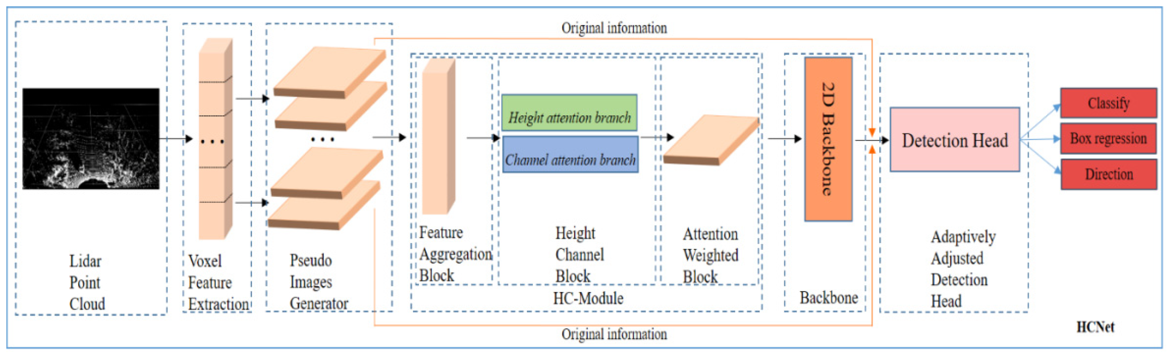
3. HCNet
- (1)
- The HC module fully aggregating the original features of the point cloud through the dual attention of height dimension and channel dimension;
- (2)
- a backbone network that uses a 2D CNN to extract features;
- (3)
- an adaptive detection-head network that adjusts the feature map and then outputs the labels and bounding boxes of the objects.
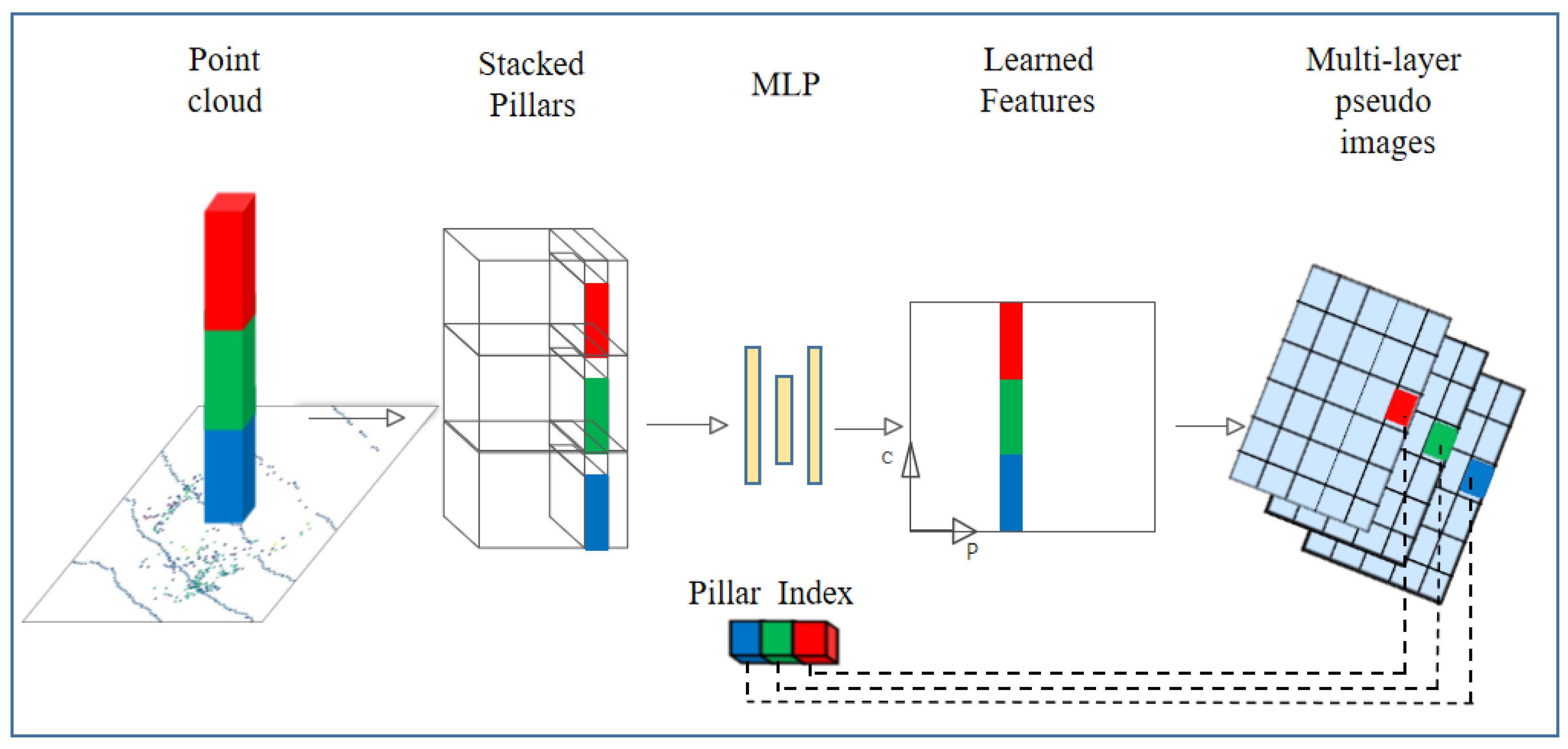
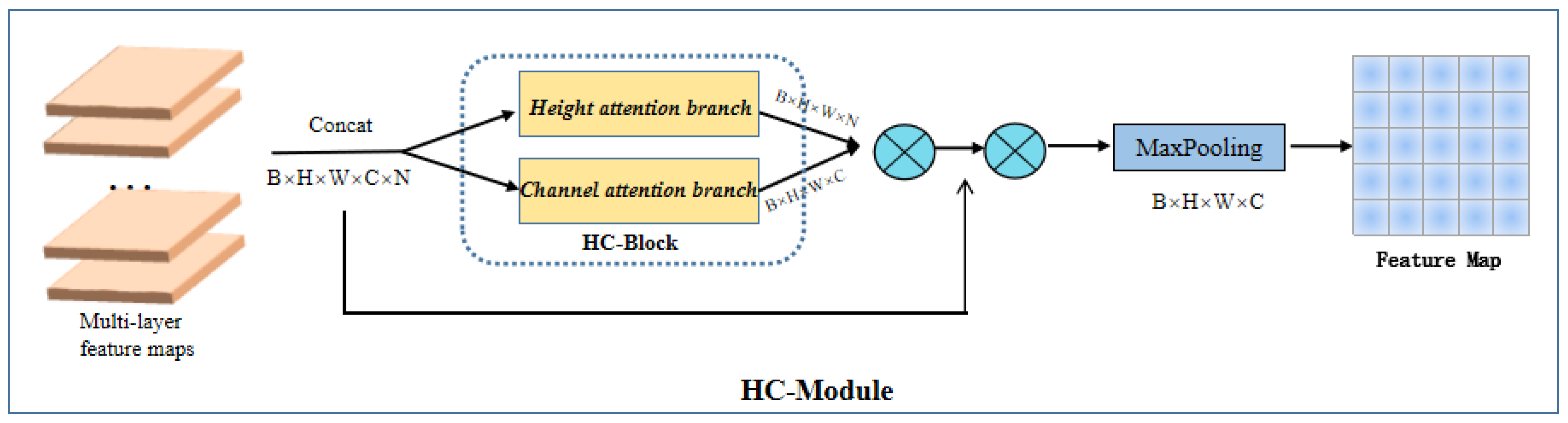
3.1. HC Module
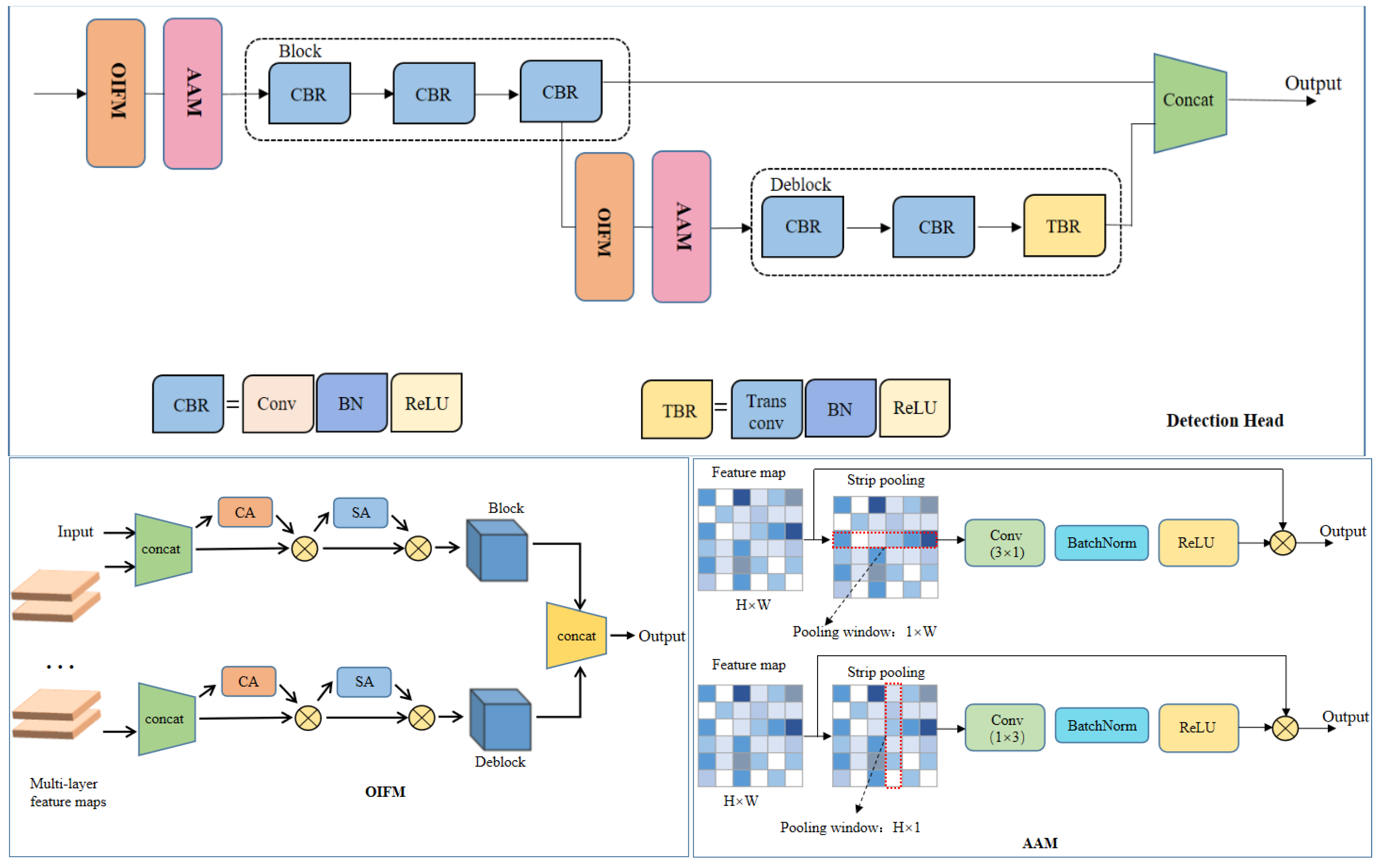
3.2. Feature Aggregation Block
3.3. HC Block
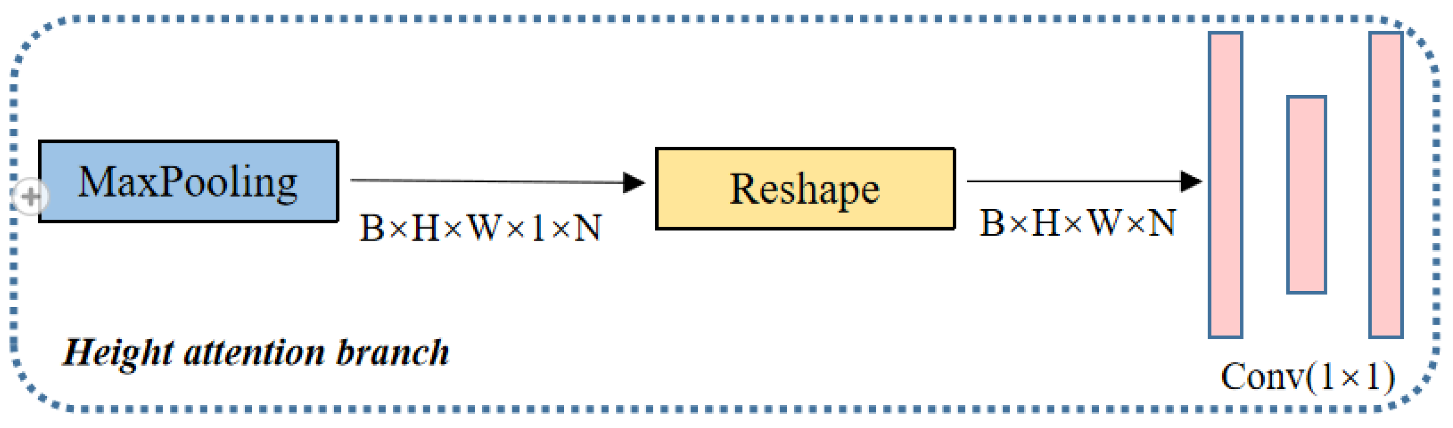
3.3.1. Height Attention Branch
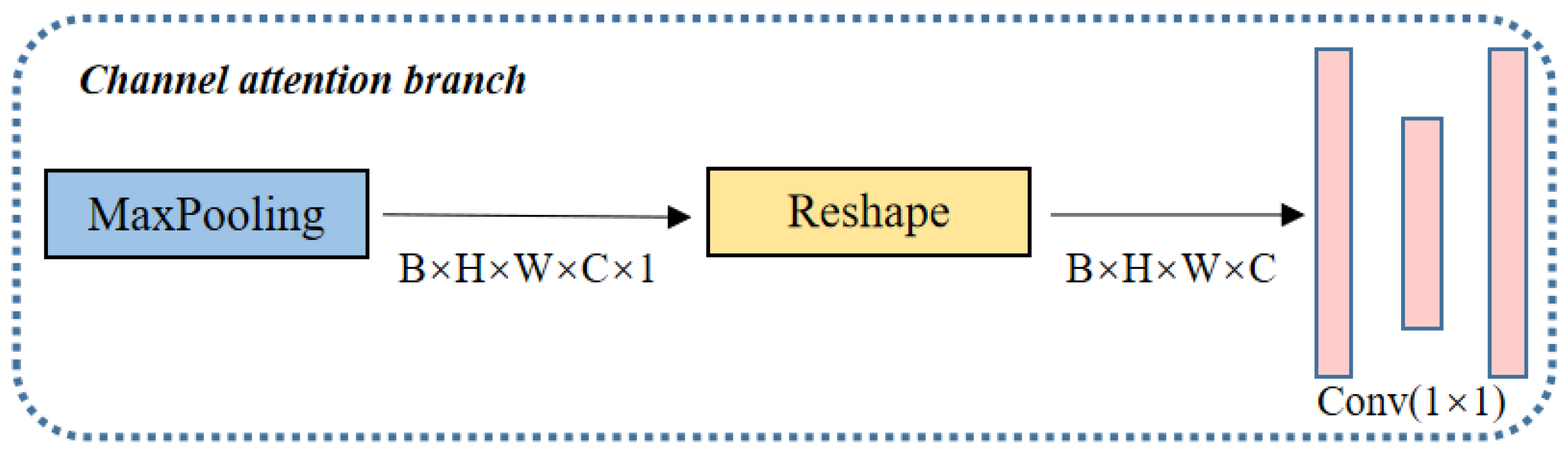
3.3.2. Channel Attention Branch
3.4. Attention-Weighted Block
3.5. Backbone
- (1)
- the top-down part, which generates features at smaller and smaller resolutions;
- (2)
- the down-top part, which up-samples the feature map from the bottom up and stitches it with the features of the upper layer;
- (3)
- the third part, which up-samples the features of each layer of the network to the same size through up-sampling, and then splices to generate the final output features.
3.6. Detection Head
3.6.1. Detection Head Backbone Network
3.6.2. Original Information-Fusion Module
3.6.3. Adaptive-Adjustment Module
3.7. Loss Function
4. Implementation Details
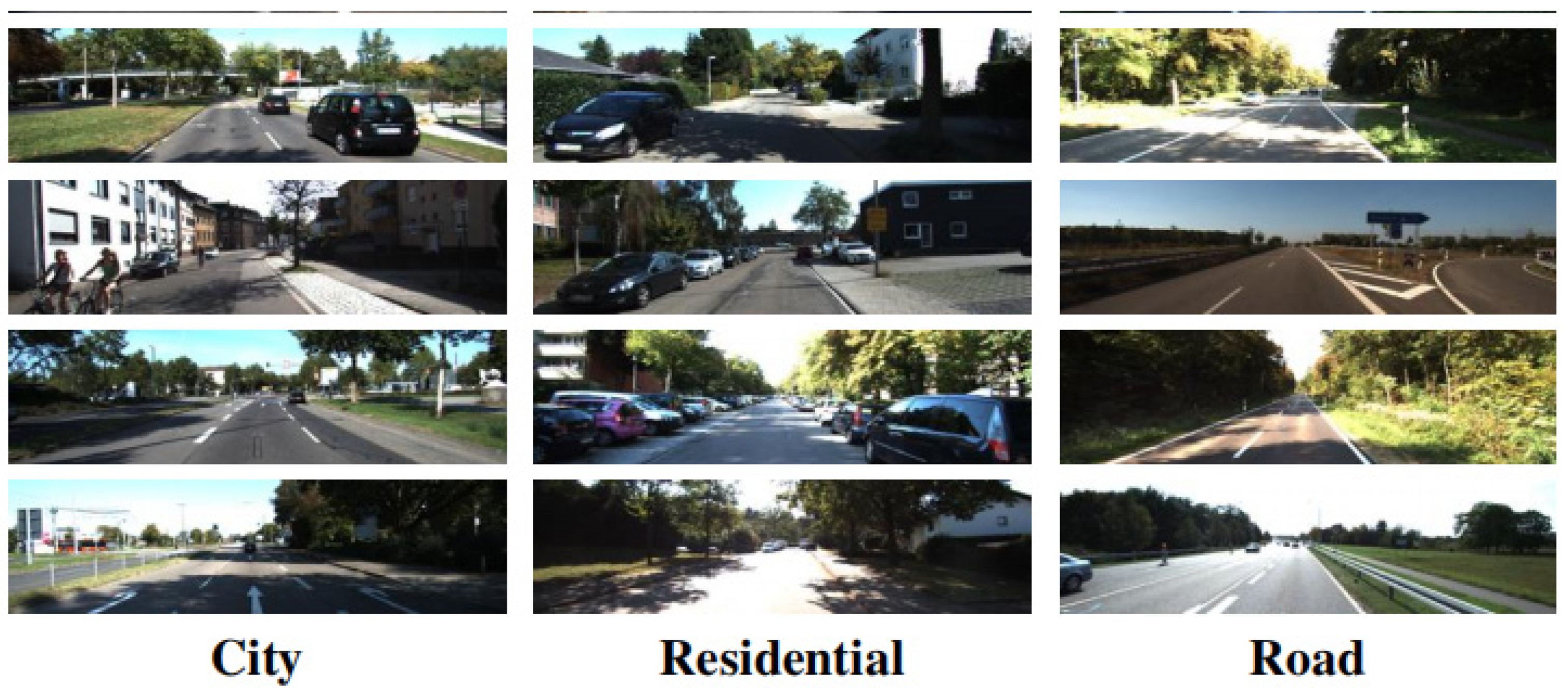
4.1. Dataset
4.2. Setting
4.3. Data Augmentation
5. Experiments
5.1. Evaluation Criteria
- (1)
- TP (True positives): Positive samples were identified as positive samples;
- (2)
- TN (True negatives): Negative samples were identified as negative samples;
- (3)
- FP (False positives): Negative samples were misidentified as positive samples;
- (4)
- FN (False negatives): Positive samples were misidentified as negative samples.
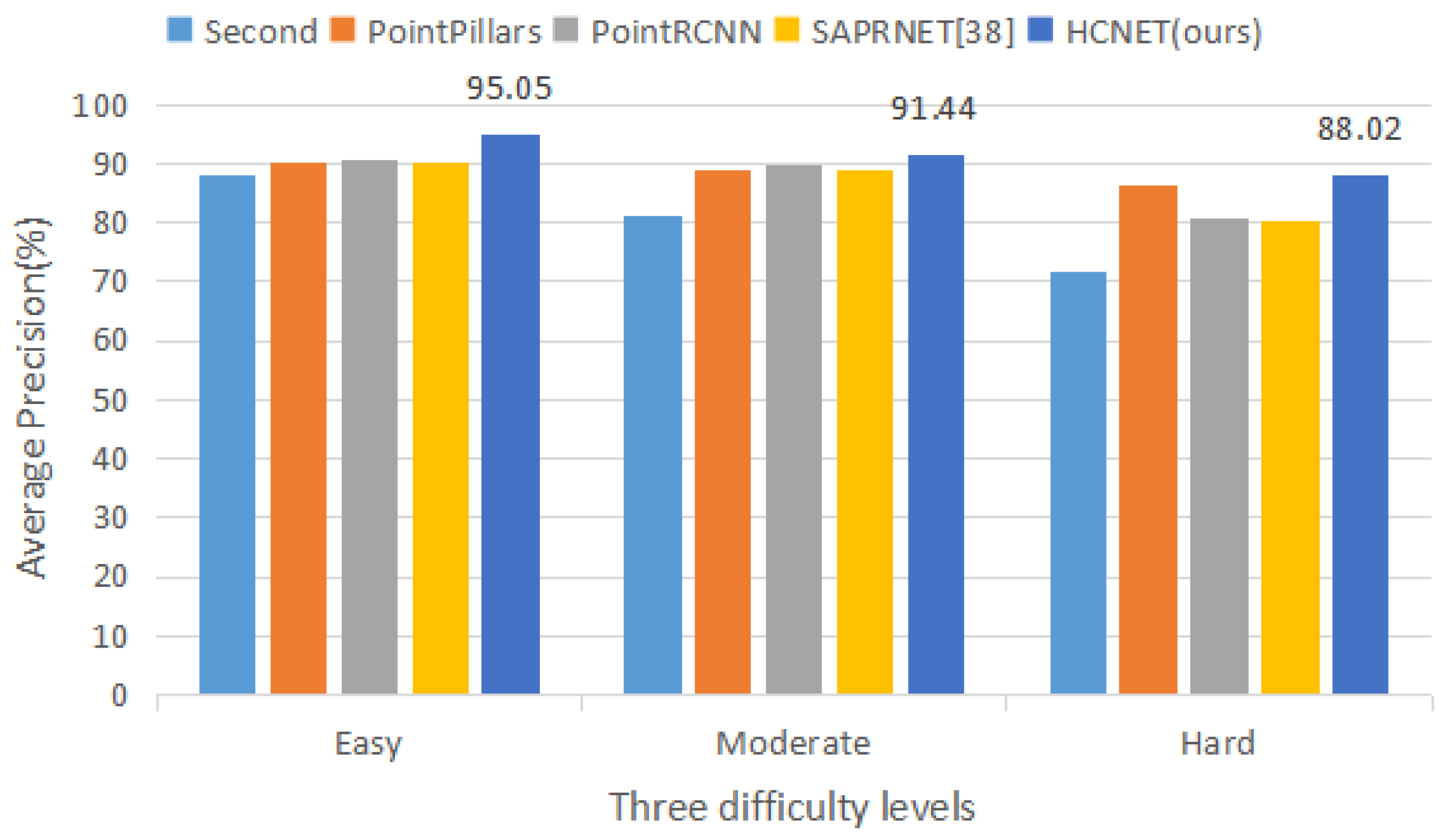
5.2. Evaluation Details
- (1)
- Our HC module focuses on more challenging tasks;
- (2)
- Our adaptive detection head overemphasizes the features of difficult objects in the distance.
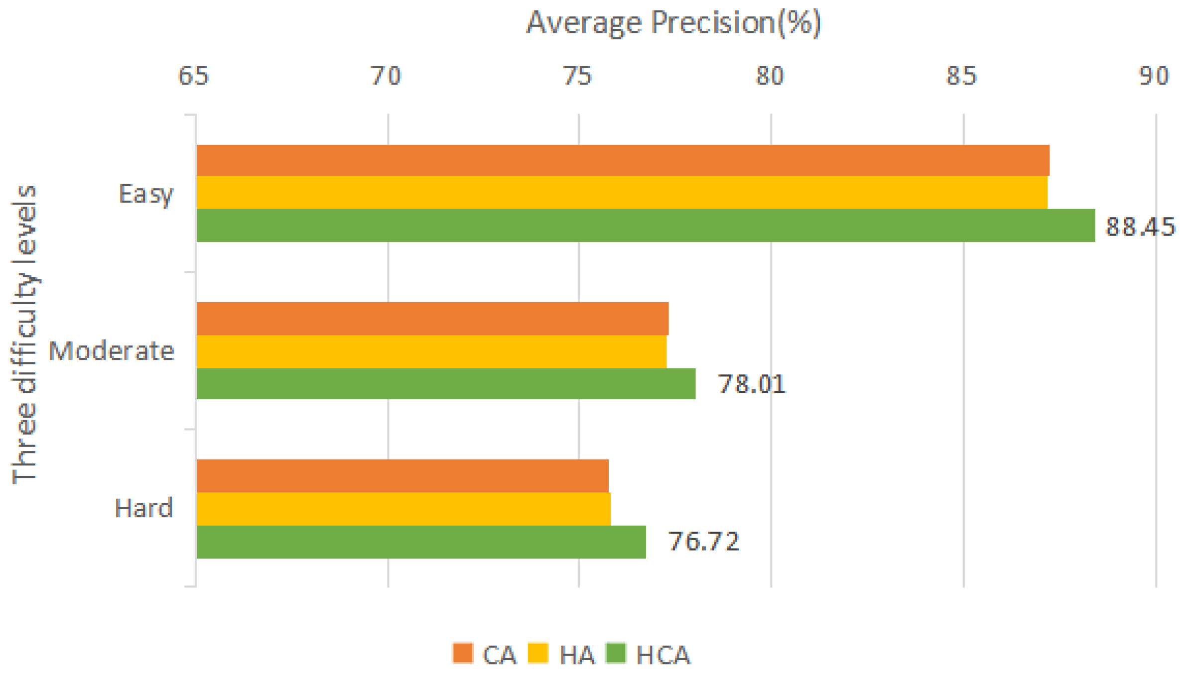
5.2.1. Different Attention Mechanisms in the HC Module
5.2.2. Different Parts of the Detection Head
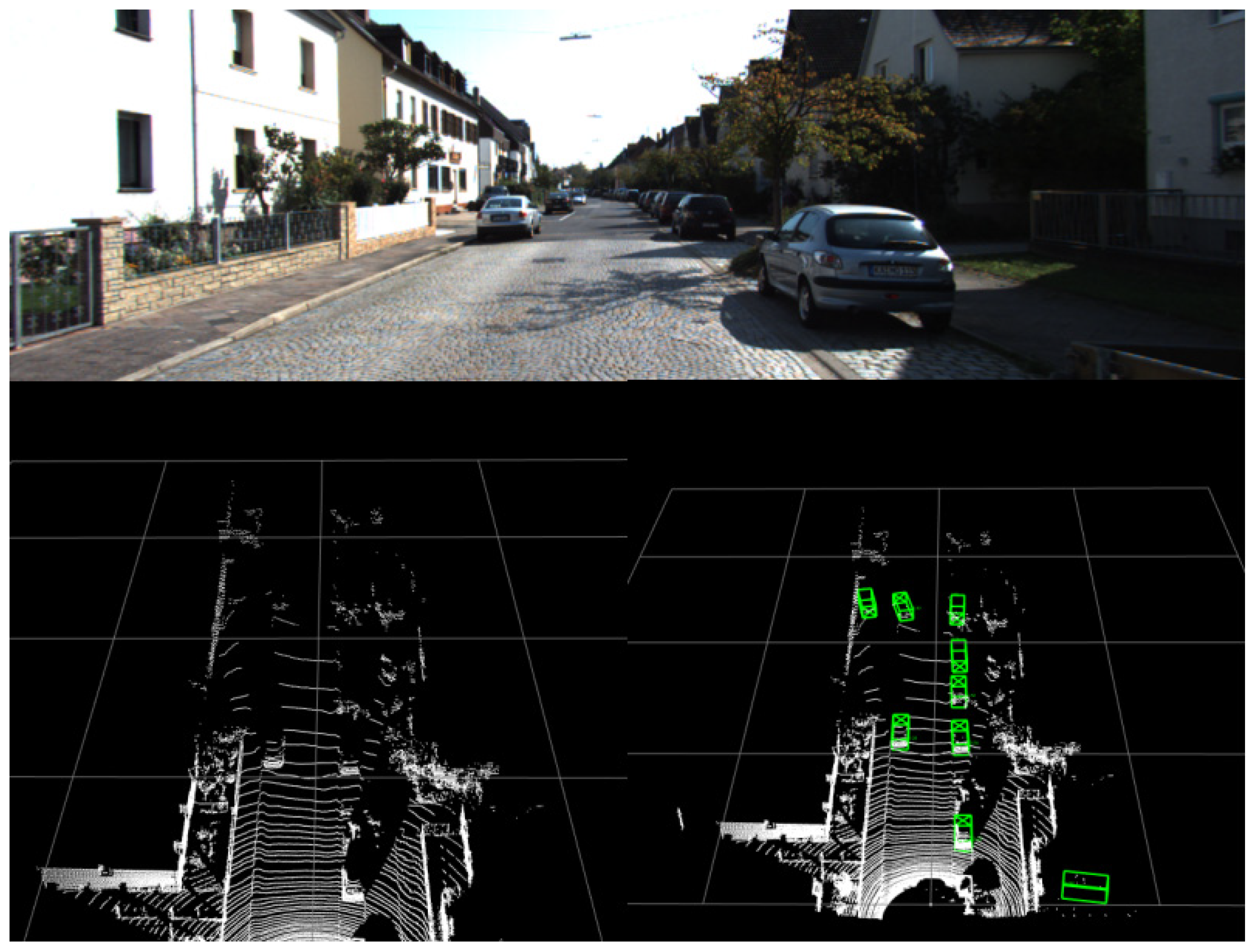
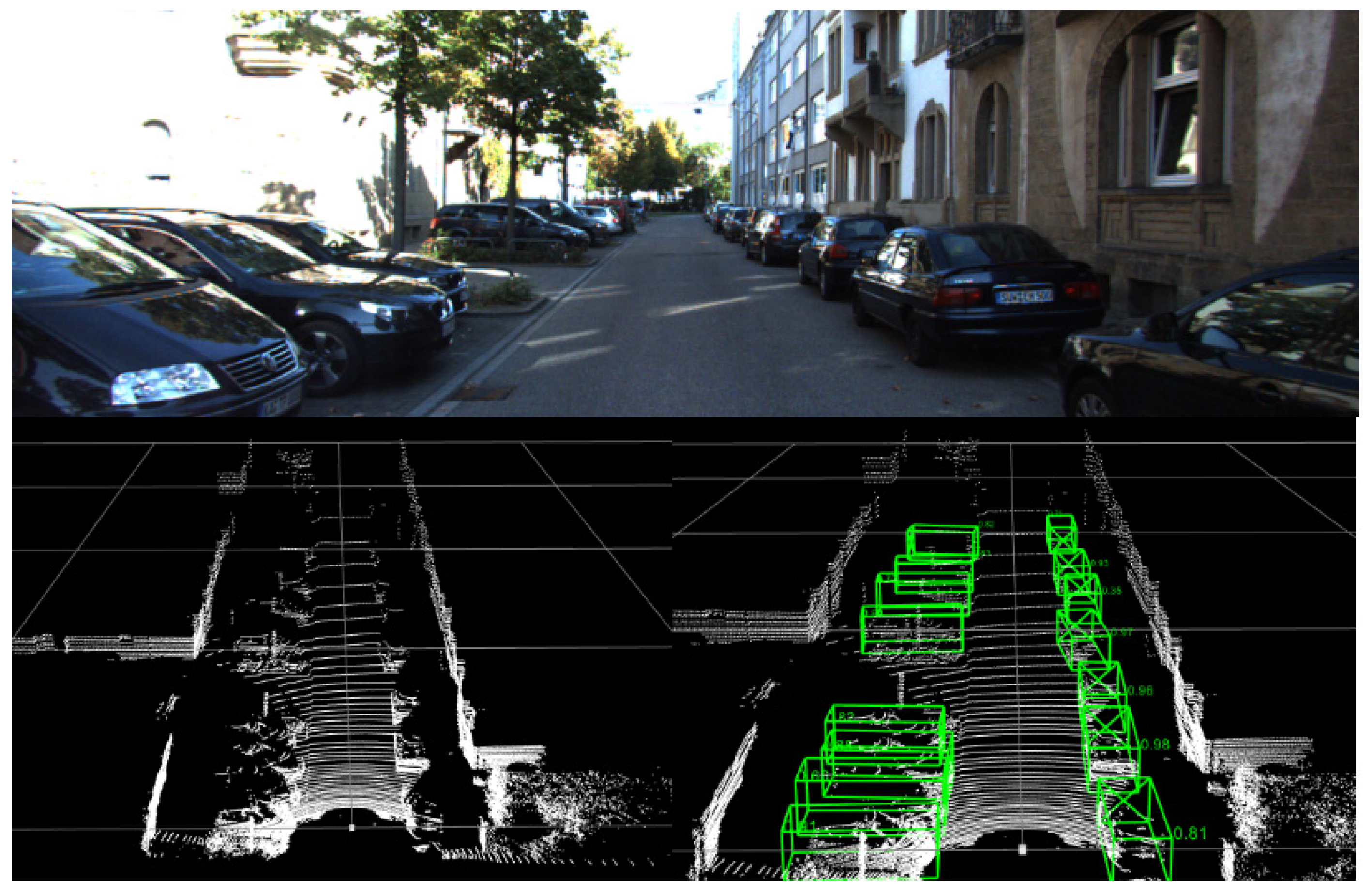
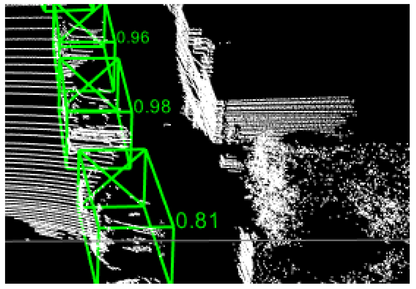
5.3. Visualization
6. Conclusions
Author Contributions
Funding
Conflicts of Interest
References
- Badue, C.; Guidolini, R.; Carneiro, R.V.; Azevedo, P.; Cardoso, V.B.; Forechi, A.; Jesus, L.; Berriel, R.; Paixao, T.M.; Mutz, F.; et al. Self-driving cars: A survey. Expert Syst. Appl. 2020, 165, 113816. [Google Scholar] [CrossRef]
- Yurtsever, E.; Lambert, J.; Carballo, A.; Takeda, K. A survey of autonomous driving: Common practices and emerging technologies. IEEE Access 2020, 8, 58443–58469. [Google Scholar] [CrossRef]
- Xiang, Y.; Choi, W.; Lin, Y.; Savarese, S. Data-driven 3d voxel patterns for object category recognition. In Proceedings of the IEEE Conference on Computer Vision and Pattern Recognition, Boston, MA, USA, 7–12 June 2015; pp. 1903–1911. [Google Scholar]
- Qi, C.R.; Su, H.; Mo, K.; Guibas, L.J. PointNet: Deep Learning on Point Sets for 3D Classification and Segmentation. In Proceedings of the IEEE Conference on Computer Vision and Pattern Recognition (CVPR), Honolulu, HI, USA, 21–26 July 2017. [Google Scholar]
- Qi, C.R.; Yi, L.; Su, H.; Guibas, L.J. Pointnet++: Deep hierarchical feature learning on point sets in a metric space. arXiv 2017, arXiv:1706.02413. [Google Scholar]
- Yin, Z.; Tuzel, O. VoxelNet: End-to-End Learning for Point Cloud Based 3D Object Detection. In Proceedings of the IEEE Conference on Computer Vision and Pattern Recognition (CVPR), Salt Lake City, UT, USA, 18–23 June 2018. [Google Scholar]
- Yan, Y.; Mao, Y.; Li, B. Second: Sparsely embedded convolutional detection. Sensors 2018, 18, 3337. [Google Scholar] [CrossRef] [Green Version]
- Lang, A.H.; Vora, S.; Caesar, H.; Zhou, L.; Yang, J.; Beijbom, O. PointPillars: Fast Encoders for Object Detection from Point Clouds. In Proceedings of the 2019 IEEE/CVF Conference on Computer Vision and Pattern Recognition (CVPR), Long Beach, CA, USA, 15–20 June 2019. [Google Scholar]
- Zhao, Z.Q.; Zheng, P.; Xu, S.T.; Wu, X. Object detection with deep learning: A review. IEEE Trans. Neural Netw. Learn. Syst. 2019, 30, 3212–3232. [Google Scholar] [CrossRef] [PubMed] [Green Version]
- Li, X.; Guivant, J.E.; Kwok, N.; Xu, Y. 3D backbone network for 3D object detection. arXiv 2019, arXiv:1901.08373. [Google Scholar]
- Li, B. 3d fully convolutional network for vehicle detection in point cloud. In Proceedings of the 2017 IEEE/RSJ International Conference on Intelligent Robots and Systems (IROS), Vancouver, BC, Canada, 24–28 September 2017; pp. 1513–1518. [Google Scholar]
- Rusu, R.B. Semantic 3d object maps for everyday manipulation in human living environments. KI-Kunstl. Intell. 2010, 24, 345–348. [Google Scholar] [CrossRef] [Green Version]
- Wang, W.; Sakurada, K.; Kawaguchi, N. Incremental and enhanced scanline-based segmentation method for surface reconstruction of sparse LiDAR data. Remote Sens. 2016, 8, 967. [Google Scholar] [CrossRef] [Green Version]
- Narksri, P.; Takeuchi, E.; Ninomiya, Y.; Morales, Y.; Akai, N.; Kawaguchi, N. A slope-robust cascaded ground segmentation in 3D point cloud for autonomous vehicles. In Proceedings of the 2018 21st International Conference on Intelligent Transportation Systems (ITSC), Maui, HI, USA, 4–7 November 2018; pp. 497–504. [Google Scholar]
- Lambert, J.; Liang, L.; Morales, L.Y.; Akai, N.; Carballo, A.; Takeuchi, E.; Narksri, P.; Seiya, S.; Takeda, K. Tsukuba challenge 2017 dynamic object tracks dataset for pedestrian behavior analysis. J. Robot. Mech. 2018, 30, 598–612. [Google Scholar] [CrossRef]
- Girshick, R.; Donahue, J.; Darrell, T.; Malik, J. Rich feature hierarchies for accurate object detection and semantic segmentation. In Proceedings of the IEEE Conference on Computer Vision and Pattern Recognition, Columbus, OH, USA, 23–28 June 2014; pp. 580–587. [Google Scholar]
- Irshick, R. Fast r-cnn. In Proceedings of the IEEE International Conference on Computer Vision, Santiago, Chile, 7–13 December 2015; pp. 1440–1448. [Google Scholar]
- Ren, S.; He, K.; Girshick, R.; Sun, J. Faster r-cnn: Towards real-time object detection with region proposal networks. arXiv 2015, arXiv:1506.01497. [Google Scholar] [CrossRef] [Green Version]
- Chen, X.; Ma, H.; Wan, J.; Li, B.; Xia, T. Multi-view 3d object detection network for autonomous driving. In Proceedings of the IEEE Conference on Computer Vision and Pattern Recognition, Honolulu, HI, USA, 21–26 July 2017; pp. 1907–1915. [Google Scholar]
- Shi, S.; Wang, X.; Li, H.P. 3d object proposal generation and detection from point cloud. In Proceedings of the IEEE Conference on Computer Vision and Pattern Recognition, Long Beach, CA, USA, 16–20 June 2019; pp. 16–20. [Google Scholar]
- Qi, C.R.; Liu, W.; Wu, C.; Su, H.; Guibas, L.J. Frustum PointNets for 3D Object Detection from RGB-D Data. In Proceedings of the IEEE Conference on Computer Vision and Pattern Recognition, Salt Lake City, UT, USA, 18–23 June 2018. [Google Scholar]
- Ali, W.; Abdelkarim, S.; Zidan, M.; Zahran, M.; El Sallab, A. YOLO3D: End-to-end real-time 3D Oriented Object Bounding Box Detection from LiDAR Point Cloud. In Proceedings of the ECCV 2018: “3D Reconstruction meets Semantics” Workshop, Munich, Germany, 8–14 September 2018. [Google Scholar]
- Redmon, J.; Divvala, S.; Girshick, R.; Farhadi, A. You only look once: Unified, real-time object detection. In Proceedings of the IEEE Conference on Computer Vision and Pattern Recognition, Las Vegas, NV, USA, 27–30 June 2016; pp. 779–788. [Google Scholar]
- Yang, Z.; Sun, Y.; Liu, S.; Jia, J. 3dssd: Point-based 3d single stage object detector. In Proceedings of the IEEE/CVF Conference on Computer Vision and Pattern Recognition, Seattle, WA, USA, 13–19 June 2020; pp. 11040–11048. [Google Scholar]
- Li, B.; Zhang, T.; Xia, T. Vehicle detection from 3d lidar using fully convolutional network. arXiv 2016, arXiv:1608.07916. [Google Scholar]
- Oda, M.; Shimizu, N.; Roth, H.R.; Karasawa, K.I.; Kitasaka, T.; Misawa, K.; Fujiwara, M.; Rueckert, D.; Mori, K. 3D FCN Feature Driven Regression Forest-Based Pancreas Localization and Segmentation. In Deep Learning in Medical Image Analysis and Multimodal Learning for Clinical Decision Support; Springer: Cham, Switzerland, 2017. [Google Scholar]
- Engelcke, M.; Rao, D.; Wang, D.Z.; Tong, C.H.; Posner, I. Vote3Deep: Fast Object Detection in 3D Point Clouds Using Efficient Convolutional Neural Networks. In Proceedings of the International Conference on Robotics and Automation (ICRA), Singapore, 29 May–3 June 2017. [Google Scholar]
- Graham, B.; Maaten, L. Submanifold Sparse Convolutional Networks. arXiv 2017, arXiv:1706.01307. [Google Scholar]
- Liu, W.; Anguelov, D.; Erhan, D.; Szegedy, C.; Reed, S.; Fu, C.Y.; Berg, A.C. Ssd: Single shot multibox detector. In European Conference on Computer Vision; Springer: Cham, Switzerland, 2016; pp. 21–37. [Google Scholar]
- Chaudhari, S.; Mithal, V.; Polatkan, G.; Ramanath, R. An Attentive Survey of Attention Models. ACM Trans. Intell. Syst. Technol. TIST 2021, 12, 1–32. [Google Scholar] [CrossRef]
- Venugopalan, S.; Rohrbach, M.; Donahue, J.; Mooney, R.; Darrell, T.; Saenko, K. Sequence to sequence-video to text. In Proceedings of the IEEE International Conference on Computer Vision, Santiago, Chile, 7–13 December 2015; pp. 4534–4542. [Google Scholar]
- Jaderberg, M.; Simonyan, K.; Zisserman, A. Spatial transformer networks. arXiv 2015, arXiv:1506.02025. [Google Scholar]
- Hu, J.; Shen, L.; Sun, G. Squeeze-and-excitation networks. In Proceedings of the IEEE Conference on Computer Vision and Pattern Recognition, Salt Lake City, UT, USA, 18–23 June 2018; pp. 7132–7141. [Google Scholar]
- Wang, F.; Jiang, M.; Qian, C.; Yang, S.; Li, C.; Zhang, H.; Wang, X.; Tang, X. Residual Attention Network for Image Classification. In Proceedings of the 2017 IEEE Conference on Computer Vision and Pattern Recognition (CVPR), Honolulu, HI, USA, 21–26 July 2017. [Google Scholar]
- Zhao, X.; Liu, Z.; Hu, R.; Huang, K. 3D object detection using scale invariant and feature reweighting networks. Proc. AAAI Conf. Artif. Intell. 2019, 33, 9267–9274. [Google Scholar] [CrossRef]
- Liu, X.; Han, Z.; Liu, Y.-S.; Zwicker, M. Point2sequence: Learning the shape representation of 3d point clouds with an attention-based sequence to sequence network. Proc. AAAI Conf. Artif. Intell. 2019, 33, 8778–8785. [Google Scholar] [CrossRef] [Green Version]
- Redmon, J.; Farhadi, A. YOLOv3: An Incremental Improvement. arXiv 2018, arXiv:1804.02767. [Google Scholar]
- Woo, S.; Park, J.; Lee, J.Y.; Kweon, I.S. Cbam: Convolutional block attention module. In Proceedings of the European Conference on Computer Vision (ECCV), Munich, Germany, 8–14 September 2018; pp. 3–19. [Google Scholar]
- Geiger, A.; Lenz, P.; Urtasun, R. Are we ready for autonomous driving? The kitti vision benchmark suite. In Proceedings of the 2012 IEEE Conference on Computer Vision and Pattern Recognition, Providence, RI, USA, 16–21 June 2012; pp. 3354–3361. [Google Scholar]
- Ye, Y.; Chen, H.; Zhang, C.; Hao, X.; Zhang, Z. SARPNET: Shape attention regional proposal network for liDAR-based 3D object detection. Neurocomputing 2020, 379, 53–63. [Google Scholar] [CrossRef]


| Method | Times(s) | 3D | ||
|---|---|---|---|---|
| Easy | Moderate | Hard | ||
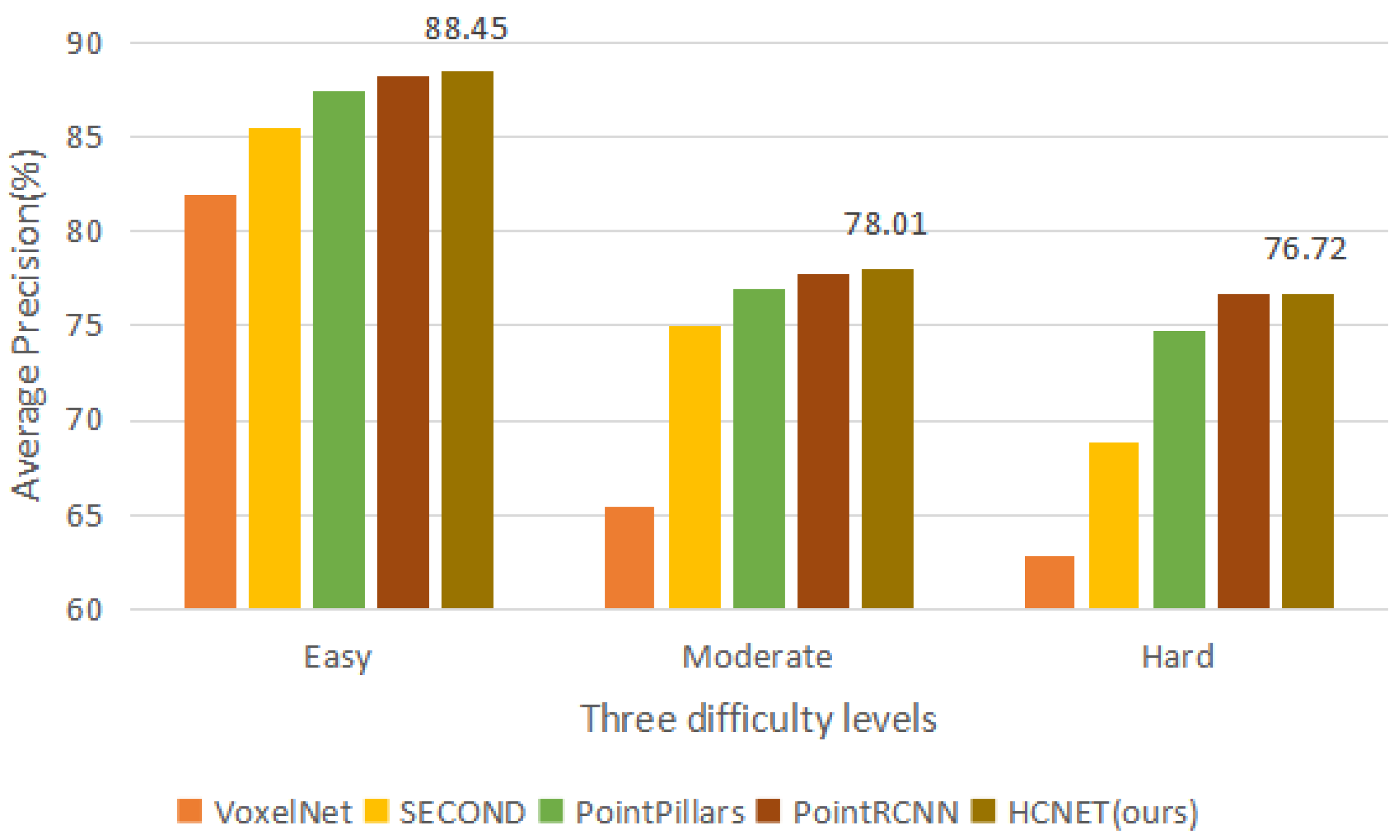
| VoxelNet [6] | 0.23 | 81.97 | 65.46 | 62.85 |
| SECOND [7] | 0.05 | 85.50 | 75.04 | 68.78 |
| PointPillars [8] | 0.016 | 87.50 | 77.01 | 74.77 |
| PointRCNN [20] | 0.10 | 88.26 | 77.73 | 76.67 |
| HCNET (ours) | 0.032 | 88.45 | 78.01 | 76.72 |
| Method | Times(s) | BEV | 3D | Orientation | ||||||
|---|---|---|---|---|---|---|---|---|---|---|
| Easy | Moderate | Hard | Easy | Moderate | Hard | Easy | Moderate | Hard | ||
| VoxelNet [6] | 0.23 | 89.35 | 79.26 | 77.39 | 77.47 | 65.11 | 57.73 | N/A | N/A | N/A |
| Second [7] | 0.05 | 88.07 | 79.37 | 77.95 | 83.13 | 73.66 | 66.20 | 87.84 | 81.31 | 71.85 |
| PointPillars [8] | 0.016 | 88.35 | 86.10 | 79.83 | 79.05 | 74.99 | 68.30 | 90.19 | 88.76 | 86.38 |
| PointRCNN [20] | 0.10 | 89.28 | 86.04 | 79.02 | 84.32 | 75.42 | 67.86 | 90.76 | 89.55 | 80.76 |
| SARPNET [40] | 0.05 | 88.93 | 87.26 | 78.68 | 84.92 | 75.64 | 67.70 | 90.16 | 88.86 | 80.05 |
| HCNET (ours) | 0.032 | 90.27 | 86.91 | 81.90 | 81.31 | 73.56 | 68.42 | 95.05 | 91.44 | 88.02 |
| Method | 3D | ||
|---|---|---|---|
| Easy | Moderate | Hard | |
| CA | 87.22 | 77.33 | 75.78 |
| HA | 87.19 | 77.26 | 75.82 |
| HCA | 88.45 | 78.01 | 76.72 |
| Method | 3D | ||
|---|---|---|---|
| Easy | Moderate | Hard | |
| AAM | 87.23 | 77.33 | 75.70 |
| OIFM | 88.32 | 78.08 | 76.52 |
| (AAM + OIFM) | 88.45 | 78.01 | 76.72 |
Publisher’s Note: MDPI stays neutral with regard to jurisdictional claims in published maps and institutional affiliations. |
© 2021 by the authors. Licensee MDPI, Basel, Switzerland. This article is an open access article distributed under the terms and conditions of the Creative Commons Attribution (CC BY) license (https://creativecommons.org/licenses/by/4.0/).
Share and Cite
Zhang, J.; Wang, J.; Xu, D.; Li, Y. HCNET: A Point Cloud Object Detection Network Based on Height and Channel Attention. Remote Sens. 2021, 13, 5071. https://doi.org/10.3390/rs13245071
Zhang J, Wang J, Xu D, Li Y. HCNET: A Point Cloud Object Detection Network Based on Height and Channel Attention. Remote Sensing. 2021; 13(24):5071. https://doi.org/10.3390/rs13245071
Chicago/Turabian StyleZhang, Jing, Jiajun Wang, Da Xu, and Yunsong Li. 2021. "HCNET: A Point Cloud Object Detection Network Based on Height and Channel Attention" Remote Sensing 13, no. 24: 5071. https://doi.org/10.3390/rs13245071
APA StyleZhang, J., Wang, J., Xu, D., & Li, Y. (2021). HCNET: A Point Cloud Object Detection Network Based on Height and Channel Attention. Remote Sensing, 13(24), 5071. https://doi.org/10.3390/rs13245071