
Disparity Estimation of High-Resolution Remote Sensing Images with Dual-Scale Matching Network


Abstract
:
1. Introduction
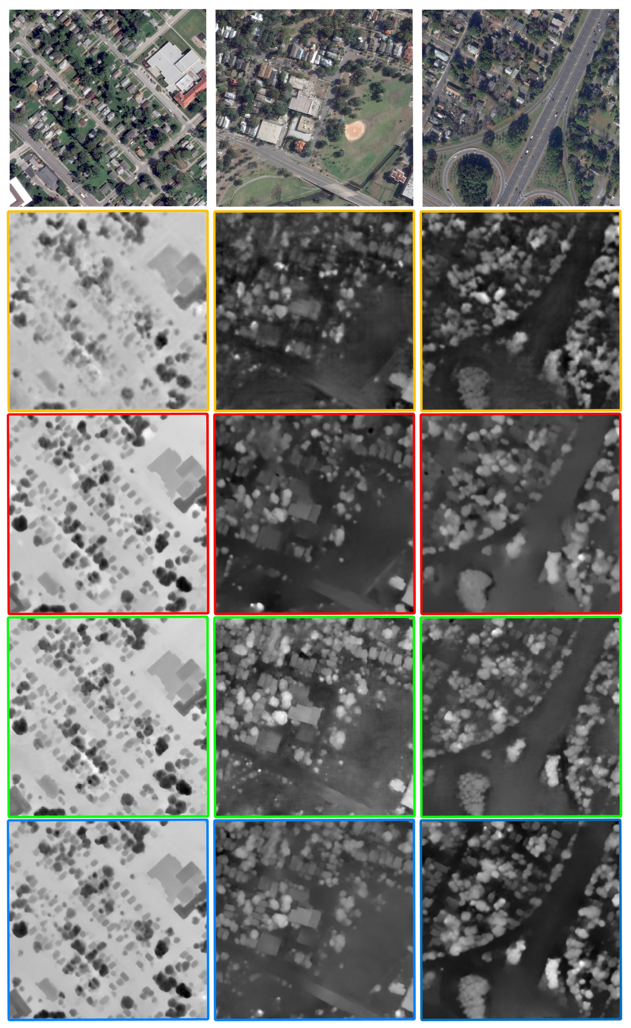
- Our network learns stereo matching at both low and high scales, helpful for disparity estimation in large areas with texture-less and repeating patterns, as well as maintenance of main structures and details.
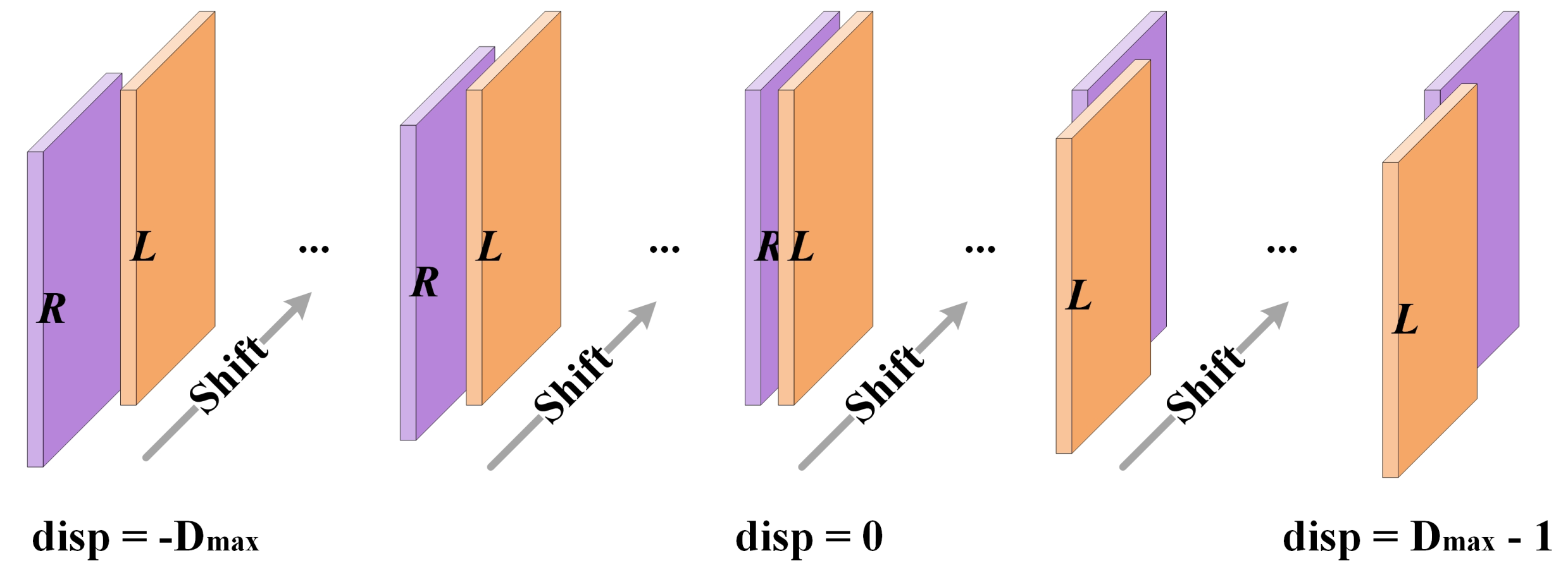
- We construct cost volumes from negative to positive values [36], making our network able to regress both negative and nonnegative disparities for remote sensing images.
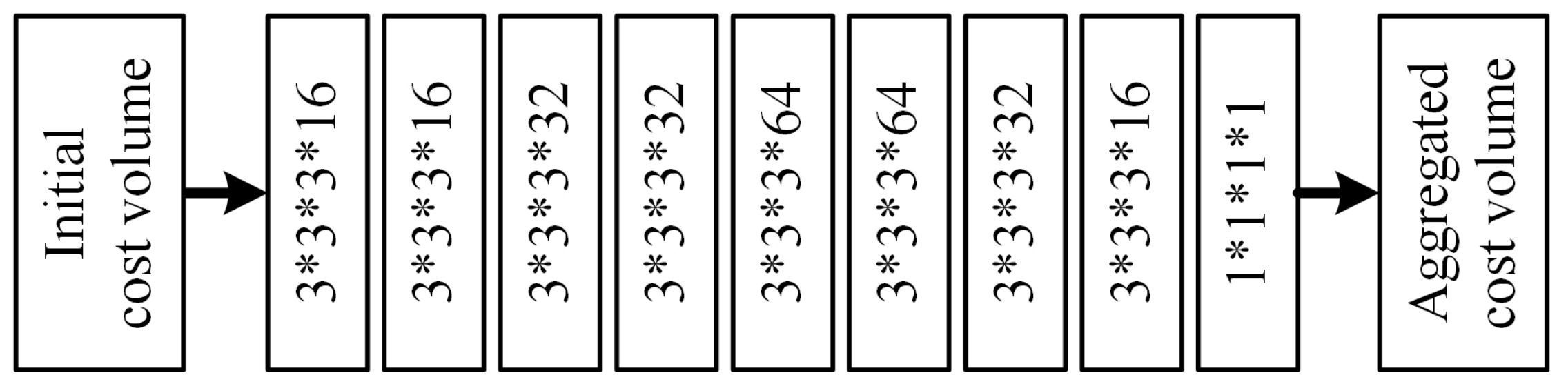
- A 3D encoder-decoder module built by factorized 3D convolutions [37] is developed for cost aggregation, which can improve the stereo matching at disparity discontinuities and occlusions. Compared with standard 3D CNNs, the computational cost is markedly reduced.
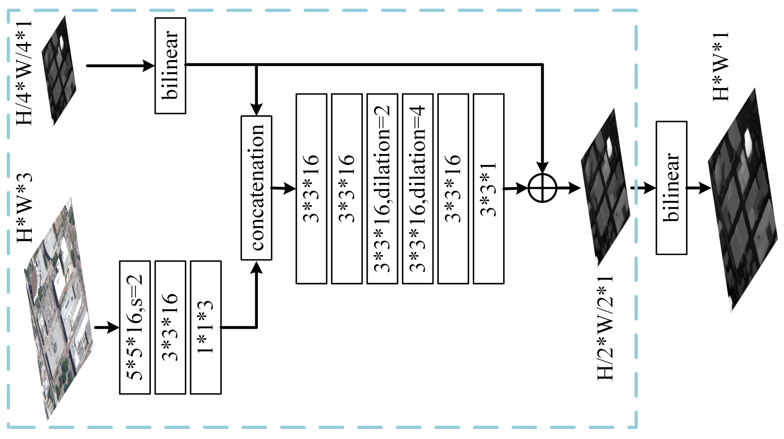
- We employ a refinement module that ensures the network outputs high-quality full-resolution disparity maps.
2. Related Work
3. Dual-Scale Matching Network
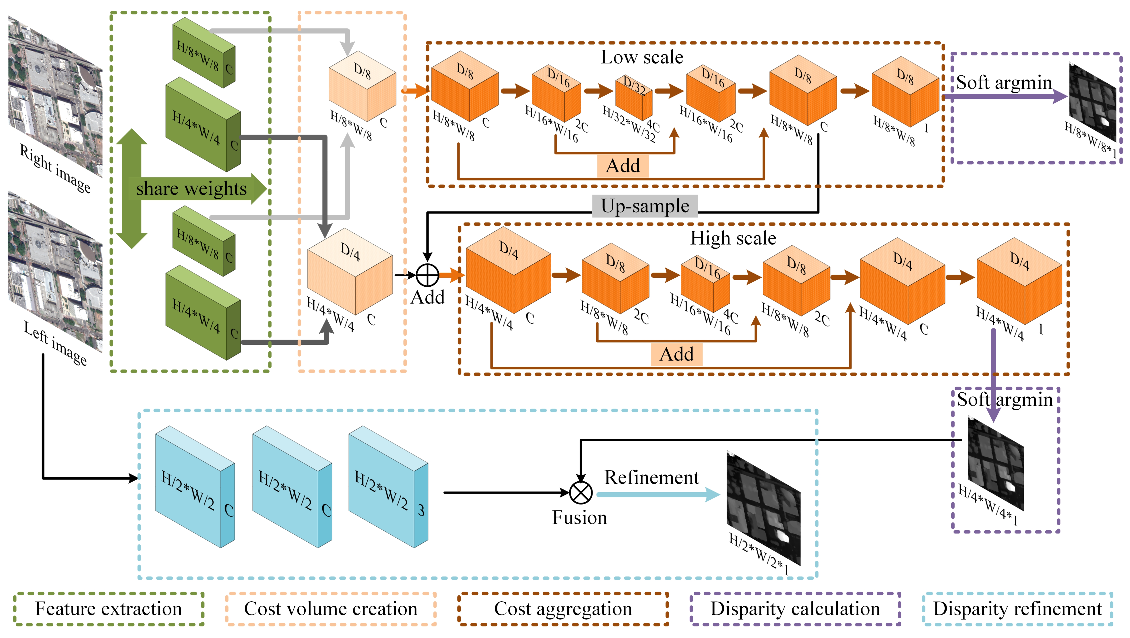
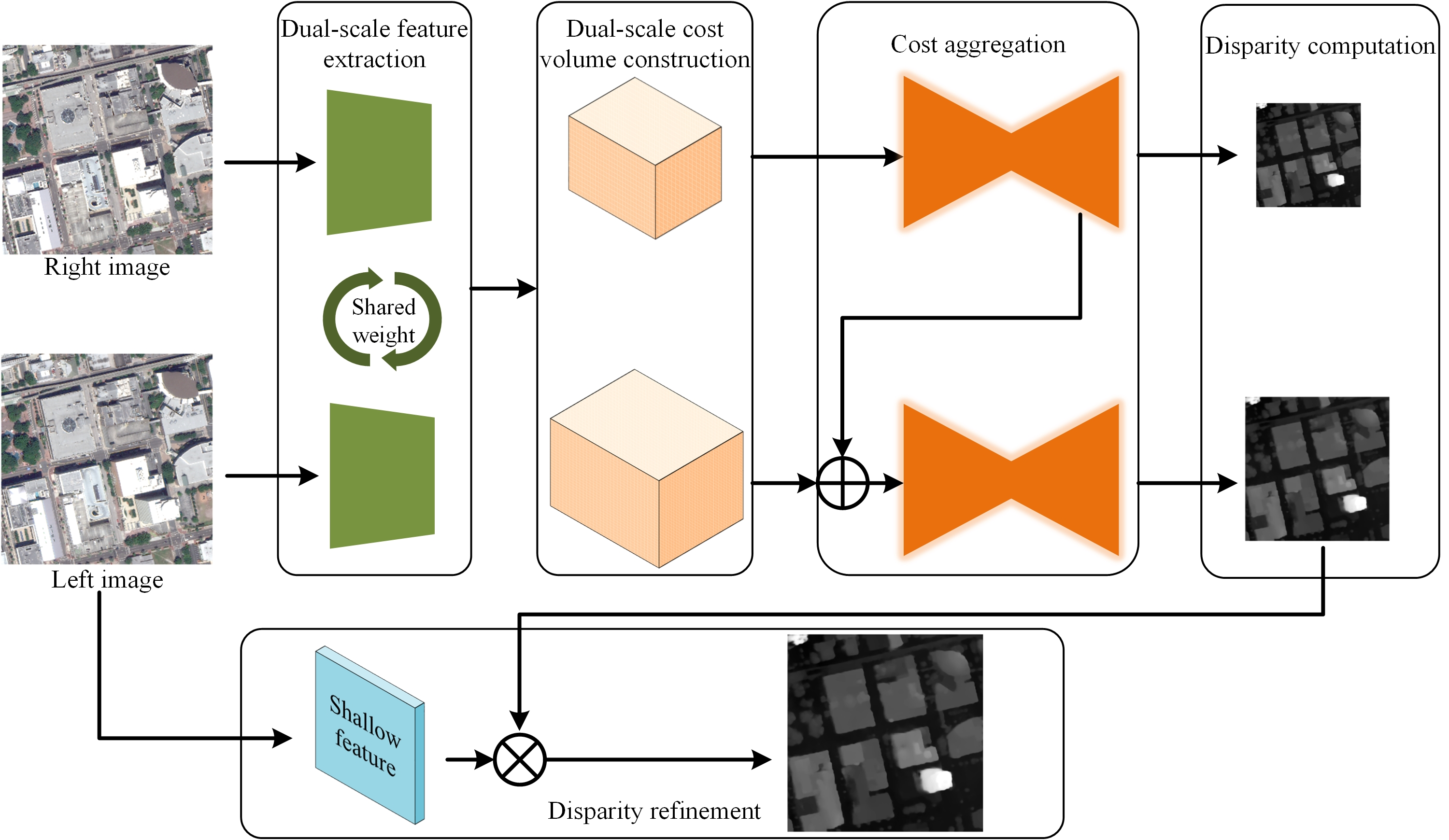
3.1. Overview
3.2. Components
3.2.1. Feature Extraction
3.2.2. Cost Volume Creation
3.2.3. Cost Aggregation
3.2.4. Disparity Calculation
3.2.5. Disparity Refinement
3.3. Loss Function
4. Experiments
4.1. Dataset and Metrics
4.2. Implementation Details
4.3. Results and Analyses
4.3.1. Overall Result
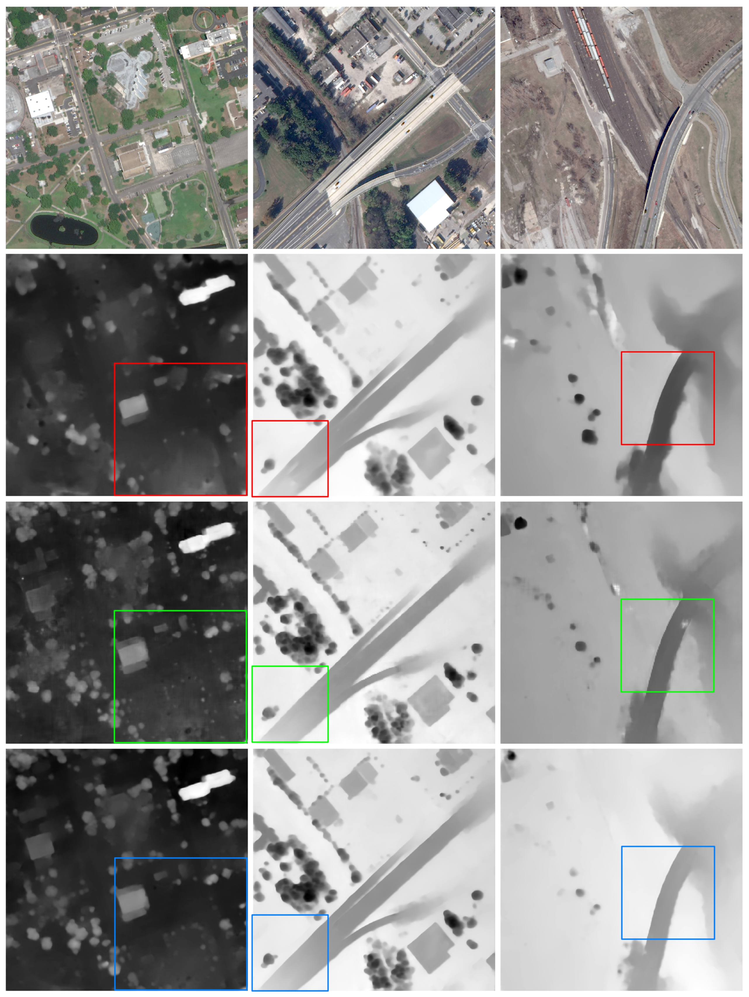
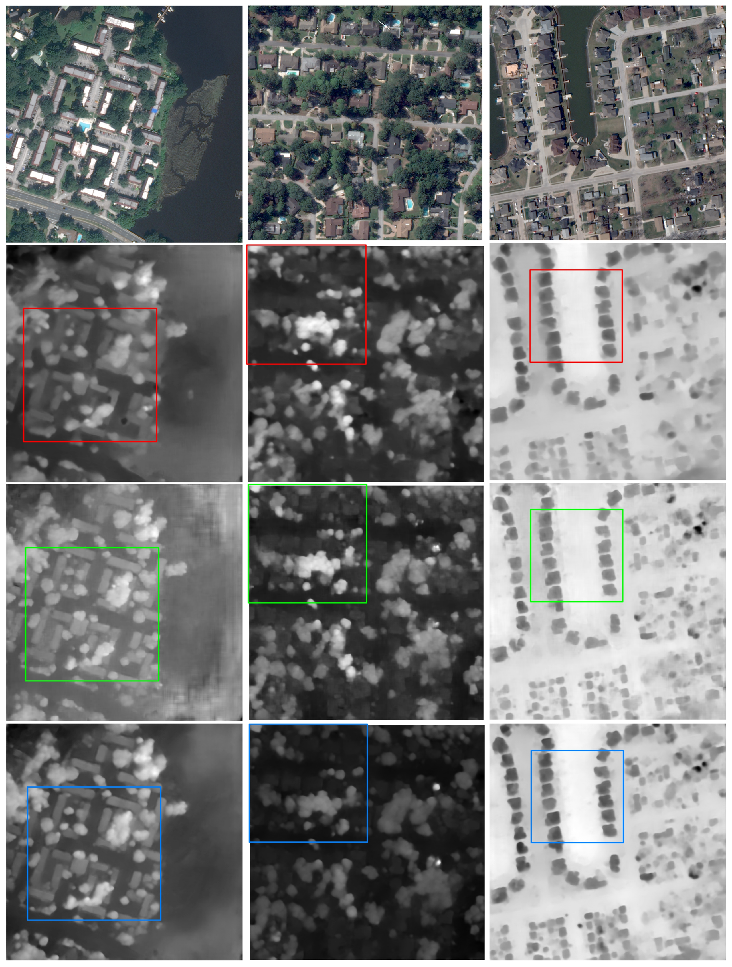
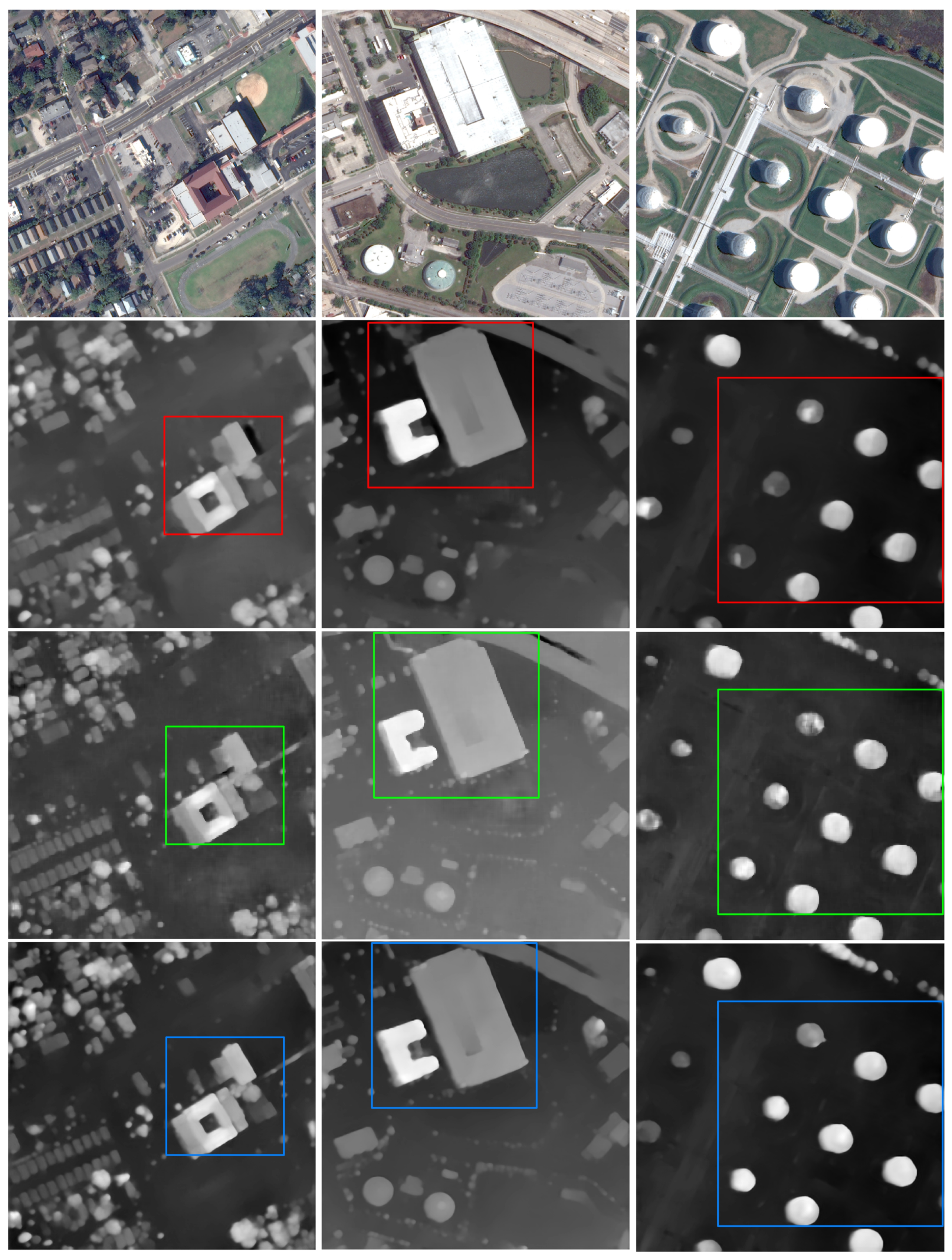
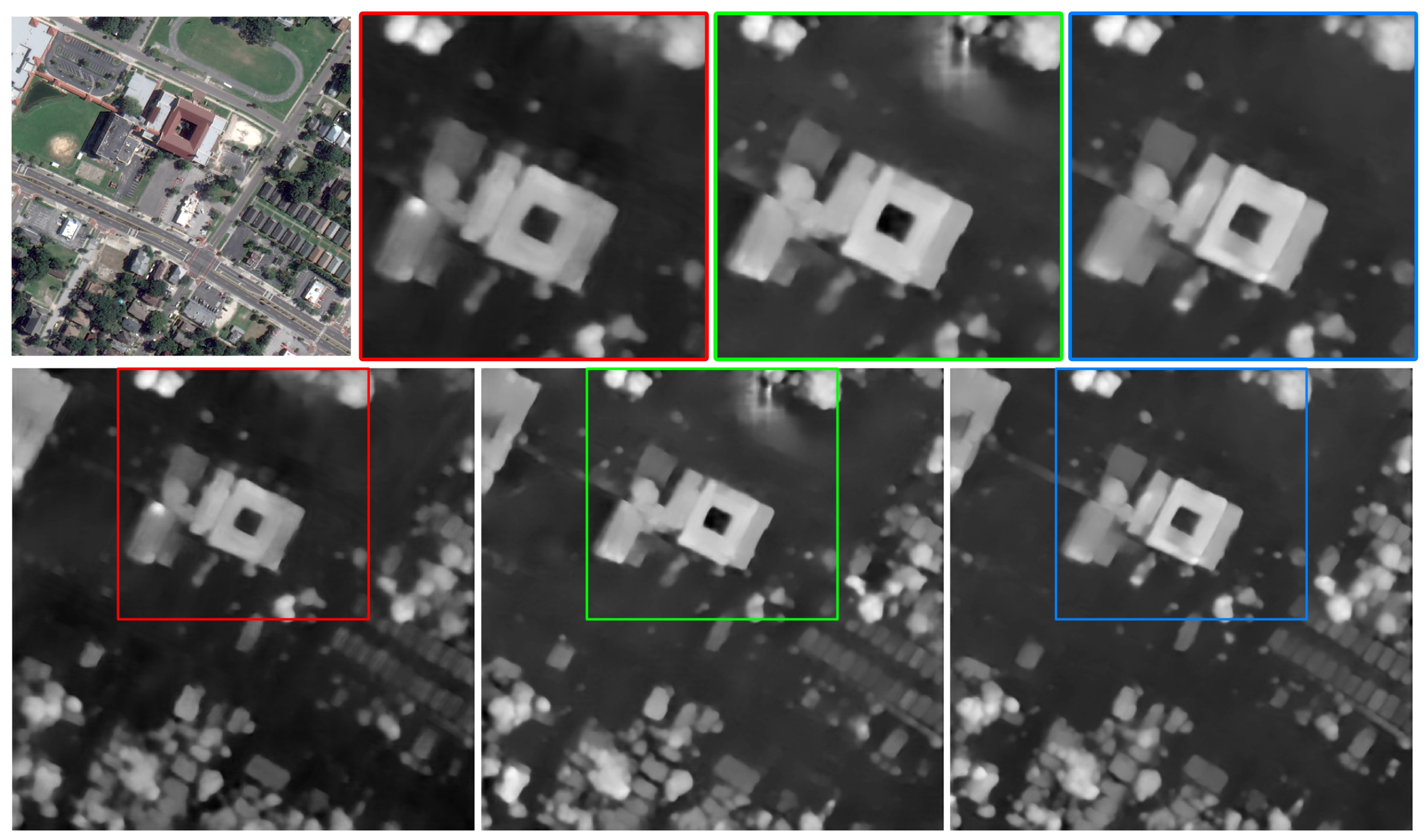
4.3.2. Result on Challenging Areas
5. Discussion
5.1. Single-Scale vs. Dual-Scale
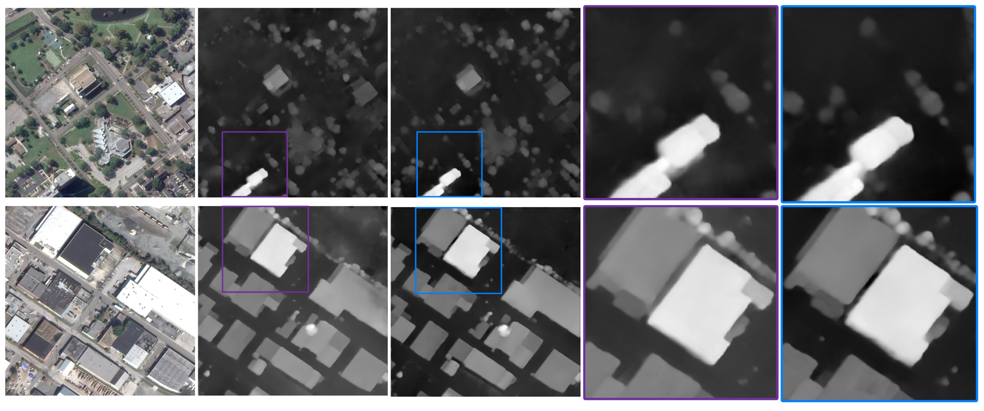
5.2. Plain Module vs. Encoder-Decoder Module
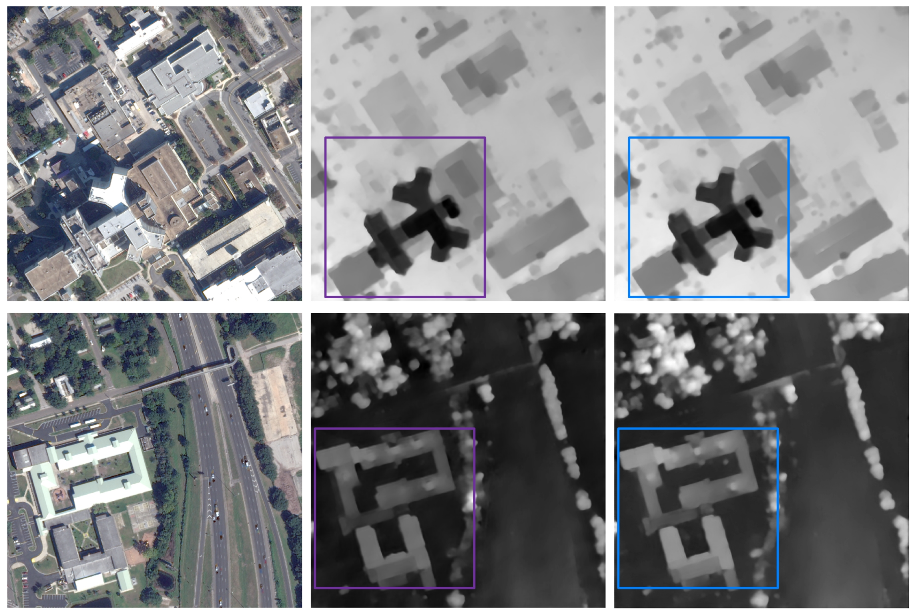
5.3. Without Refinement vs. With Refinement
6. Conclusions
Author Contributions
Funding
Institutional Review Board Statement
Informed Consent Statement
Data Availability Statement
Acknowledgments
Conflicts of Interest
References
- Kang, J.H.; Chen, L.; Deng, F.; Heipke, C. Context pyramidal network for stereo matching regularized by disparity gradients. ISPRS-J. Photogramm. Remote Sens. 2019, 157, 201–215. [Google Scholar] [CrossRef]
- Hirschmuller, H. Accurate and efficient stereo processing by semi-global matching and mutual information. In Proceedings of the IEEE Conference on Computer Vision and Pattern Recognition, San Diego, CA, USA, 20–25 June 2005; pp. 807–814. [Google Scholar]
- Zhang, L.; Seitz, S.M. Estimating optimal parameters for MRF stereo from a single image pair. IEEE Trans. Pattern Anal. Mach. Intell. 2007, 29, 331–342. [Google Scholar] [CrossRef] [PubMed] [Green Version]
- Hirschmueller, H.; Scharstein, D. Evaluation of cost functions for stereo matching. In Proceedings of the IEEE Conference on Computer Vision and Pattern Recognition, Minneapolis, MO, USA, 17–22 June 2007. [Google Scholar]
- Rhemann, C.; Hosni, A.; Bleyer, M.; Rother, C.; Gelautz, M. Fast Cost-Volume Filtering for Visual Correspondence and Beyond. In Proceedings of the IEEE Conference on Computer Vision and Pattern Recognition, Colorado Springs, CO, USA, 20–25 June 2011. [Google Scholar]
- Scharstein, D.; Szeliski, R. A taxonomy and evaluation of dense two-frame stereo correspondence algorithms. Int. J. Comput. Vis. 2002, 47, 7–42. [Google Scholar] [CrossRef]
- Krizhevsky, A.; Sutskever, I.; Hinton, G.E. ImageNet Classification with Deep Convolutional Neural Networks. Commun. ACM. 2017, 60, 84–90. [Google Scholar] [CrossRef]
- Shelhamer, E.; Long, J.; Darrell, T. Fully Convolutional Networks for Semantic Segmentation. IEEE Trans. Pattern Anal. Mach. Intell. 2017, 39, 640–651. [Google Scholar] [CrossRef] [PubMed]
- Girshick, R.; Donahue, J.; Darrell, T.; Malik, J. Rich feature hierarchies for accurate object detection and semantic segmentation. In Proceedings of the IEEE Conference on Computer Vision and Pattern Recognition, Columbus, GA, USA, 23–28 June 2014; pp. 580–587. [Google Scholar]
- Eigen, D.; Puhrsch, C.; Fergus, R. Depth Map Prediction from a Single Image using a Multi-Scale Deep Network. In Proceedings of the Conference on Neural Information Processing Systems, Montreal, WI, USA, 8–13 December 2014. [Google Scholar]
- Zbontar, J.; LeCun, Y. Stereo Matching by Training a Convolutional Neural Network to Compare Image Patches. J. Mach. Learn. Res. 2016, 17, 65. [Google Scholar]
- Luo, W.J.; Schwing, A.G.; Urtasun, R. Efficient Deep Learning for Stereo Matching. In Proceedings of the IEEE Conference on Computer Vision and Pattern Recognition, Seattle, WA, USA, 27–30 June 2016; pp. 5695–5703. [Google Scholar]
- Park, H.; Lee, K.M. Look Wider to Match Image Patches With Convolutional Neural Networks. IEEE Signal Process. Lett. 2017, 24, 1788–1792. [Google Scholar] [CrossRef] [Green Version]
- Seki, A.; Pollefeys, M. Patch based confidence prediction for dense disparity map. In Proceedings of the British Machine Vision Conference, York, UK, 19–22 September 2016. [Google Scholar]
- Seki, A.; Pollefeys, M. SGM-Nets: Semi-global matching with neural networks. In Proceedings of the IEEE Conference on Computer Vision and Pattern Recognition, Honolulu, HI, USA, 21–26 July 2017; pp. 6640–6649. [Google Scholar]
- Shaked, A.; Wolf, L. Improved Stereo Matching with Constant Highway Networks and Reflective Confidence Learning. In Proceedings of the IEEE Conference on Computer Vision and Pattern Recognition, Honolulu, HI, USA, 21–27 July 2017; pp. 6901–6910. [Google Scholar]
- Ye, X.Q.; L, J.M.; Wang, H.; Huang, H.X.; Zhang, X.L. Efficient Stereo Matching Leveraging Deep Local and Context Information. IEEE Access. 2017, 5, 18745–18755. [Google Scholar] [CrossRef]
- Poggi, M.; Tosi, F.; Batsos, K.; Mordohai, P.; Mattoccia, S. On the Synergies between Machine Learning and Binocular Stereo for Depth Estimation from Images: A Survey. IEEE Trans. Pattern Anal. Mach. Intell. 2021. [Google Scholar] [CrossRef] [PubMed]
- Liang, Z.F.; Feng, Y.L.; Guo, Y.L.; Liu, H.Z.; Chen, W.; Qiao, L.B.; Zhou, L.; Zhang, J.F. Learning for Disparity Estimation through Feature Constancy. In Proceedings of the IEEE Conference on Computer Vision and Pattern Recognition, Salt Lake City, UT, USA, 18–23 June 2018; pp. 2811–2820. [Google Scholar]
- Mayer, N.; Ilg, E.; Hausser, P.; Fischer, P.; Cremers, D.; Dosovitskiy, A.; Brox, T. A Large Dataset to Train Convolutional Networks for Disparity, Optical Flow, and Scene Flow Estimation. In Proceedings of the IEEE Conference on Computer Vision and Pattern Recognition, Seattle, WA, USA, 27–30 June 2016; pp. 4040–4048. [Google Scholar]
- Dosovitskiy, A.; Fischer, P.; Ilg, E.; Haeusser, P.; Hazirbas, C.; Golkov, V.; van der Smagt, P.; Cremers, D.; Brox, T. FlowNet: Learning Optical Flow with Convolutional Networks. In Proceedings of the IEEE International Conference on Computer Vision, Santiago, Chile, 11–18 December 2015; pp. 2758–2766. [Google Scholar]
- Kendall, A.; Martirosyan, H.; Dasgupta, S.; Henry, P.; Kennedy, R.; Bachrach, A.; Bry, A. End-to-End Learning of Geometry and Context for Deep Stereo Regression. In Proceedings of the IEEE International Conference on Computer Vision, Venice, Italy, 22–29 October 2017; pp. 66–75. [Google Scholar]
- Pang, J.H.; Sun, W.X.; Ren, J.S.J.; Yang, C.X.; Yan, Q. Cascade Residual Learning: A Two-stage Convolutional Neural Network for Stereo Matching. In Proceedings of the IEEE International Conference on Computer Vision, Venice, Italy, 22–29 October 2017; pp. 878–886. [Google Scholar]
- Tonioni, A.; Tosi, F.; Poggi, M.; Mattoccia, S.; di Stefano, L. Real-time self-adaptive deep stereo. In Proceedings of the IEEE Conference on Computer Vision and Pattern Recognition, Long Beach, CA, USA, 16–20 June 2019; pp. 195–204. [Google Scholar]
- Xu, H.F.; Zhang, J.Y. AANet: Adaptive Aggregation Network for Efficient Stereo Matching. In Proceedings of the IEEE Conference on Computer Vision and Pattern Recognition, Electr Network, 14–19 June 2020; pp. 1956–1965. [Google Scholar]
- Chang, J.R.; Chen, Y.S. Pyramid Stereo Matching Network. In Proceedings of the IEEE Conference on Computer Vision and Pattern Recognition, Salt Lake City, UT, USA, 18–23 June 2018; pp. 5410–5418. [Google Scholar]
- Khamis, S.; Fanello, S.; Rhemann, C.; Kowdle, A.; Valentin, J.; Izadi, S. StereoNet: Guided Hierarchical Refinement for Real-Time Edge-Aware Depth Prediction. In Proceedings of the European Conference on Computer Vision, Munich, Germany, 8–14 September 2018; pp. 596–613. [Google Scholar]
- Yu, L.D.; Wang, Y.C.; Wu, Y.W.; Jia, Y.D. Deep Stereo Matching with Explicit Cost Aggregation Sub-Architecture. In Proceedings of the Innovative Applications of Artificial Intelligence Conference, New Orleans, LA, USA, 2–7 February 2018; pp. 7517–7524. [Google Scholar]
- Chabra, R.; Straub, J.; Sweeney, C.; Newcombe, R.; Fuchs, H. StereoDRNet: Dilated Residual StereoNet. In Proceedings of the IEEE Conference on Computer Vision and Pattern Recognition, Long Beach, CA, USA, 16–20 June 2019; pp. 11778–11787. [Google Scholar]
- Xing, J.B.; Qi, Z.; Dong, J.Y.; Cai, J.X.; Liu, H. MABNet: A Lightweight Stereo Network Based on Multibranch Adjustable Bottleneck Module. In Proceedings of the European Conference on Computer Vision, Glasgow, UK, 23–28 August 2020; pp. 340–356. [Google Scholar]
- Geiger, A.; Lenz, P.; Urtasun, R. Are we ready for autonomous driving? The KITTI vision benchmark suite. In Proceedings of the IEEE Conference on Computer Vision and Pattern Recognition, Providence, RI, USA, 16–21 June 2012; pp. 2018–2025. [Google Scholar]
- Menze, M.; Geiger, A. Object Scene Flow for Autonomous Vehicles. In Proceedings of the IEEE Conference on Computer Vision and Pattern Recognition, Boston, MA, USA, 7–12 June 2015; pp. 3061–3070. [Google Scholar]
- Scharstein, D.; Hirschmüller, H.; Kitajima, Y.; Krathwohl, G.; Nešić, N.; Wang, X.; Westling, P. High-Resolution Stereo Datasets with Subpixel-Accurate Ground Truth. In Proceedings of the German Conference on Pattern Recognition, Münster, Germany, 2–5 September 2014; pp. 31–42. [Google Scholar]
- Mayer, N.; Ilg, E.; Fischer, P.; Hazirbas, C.; Cremers, D.; Dosovitskiy, A.; Brox, T. What Makes Good Synthetic Training Data for Learning Disparity and Optical Flow Estimation? Int. J. Comput. Vis. 2018, 126, 942–960. [Google Scholar] [CrossRef] [Green Version]
- Ji, S.P.; Liu, J.; Lu, M. CNN-Based Dense Image Matching for Aerial Remote Sensing Images. Photogramm. Eng. Remote Sens. 2019, 85, 415–424. [Google Scholar] [CrossRef]
- Tao, R.S.; Xiang, Y.M.; You, H.J. An Edge-Sense Bidirectional Pyramid Network for Stereo Matching of VHR Remote Sensing Images. Remote Sens. 2020, 12, 4025. [Google Scholar] [CrossRef]
- Tran, D.; Wang, H.; Torresani, L.; Ray, J.; LeCun, Y.; Paluri, M. A Closer Look at Spatiotemporal Convolutions for Action Recognition. In Proceedings of the IEEE Conference on Computer Vision and Pattern Recognition, Salt Lake City, UT, USA, 18–23 June 2018; pp. 6450–6459. [Google Scholar]
- He, K.M.; Zhang, X.Y.; Ren, S.Q.; Sun, J. Spatial Pyramid Pooling in Deep Convolutional Networks for Visual Recognition. IEEE Trans. Pattern Anal. Mach. Intell. 2015, 37, 1904–1916. [Google Scholar] [CrossRef] [PubMed] [Green Version]
- Chopra, S.; Hadsell, R.; LeCun, Y. Learning a similarity metric discriminatively, with application to face verification. In Proceedings of the IEEE Conference on Computer Vision and Pattern Recognition, San Diego, CA, USA, 20–25 June 2005; pp. 539–546. [Google Scholar]
- He, K.M.; Zhang, X.Y.; Ren, S.Q.; Sun, J. Deep Residual Learning for Image Recognition. In Proceedings of the IEEE Conference on Computer Vision and Pattern Recognition, Seattle, WA, USA, 27–30 June 2016; pp. 770–778. [Google Scholar]
- Ioffe, S.; Szegedy, C. Batch Normalization: Accelerating Deep Network Training by Reducing Internal Covariate Shift. In Proceedings of the International Conference on Machine Learning, Lille, France, 7–9 July 2015; pp. 448–456. [Google Scholar]
- Zeiler, M.D.; Taylor, G.W.; Fergus, R. Adaptive Deconvolutional Networks for Mid and High Level Feature Learning. In Proceedings of the IEEE International Conference on Computer Vision, Barcelona, Spain, 6–13 November 2011; pp. 2018–2025. [Google Scholar]
- Fisher, Y.; Vladlen, K. Multi-Scale Context Aggregation by Dilated Convolutions. arXiv 2015, arXiv:1511.07122. Available online: https://arxiv.org/abs/1511.07122 (accessed on 23 November 2015).
- Girshick, R. Fast R-CNN. In Proceedings of the IEEE International Conference on Computer Vision, Santiago, Chile, 11–18 December 2015; pp. 1440–1448. [Google Scholar]
- Bosch, M.; Foster, K.; Christie, G.; Wang, S.; Hager, G.D.; Brown, M. Semantic Stereo for Incidental Satellite Images. In Proceedings of the IEEE Winter Conference on Applications of Computer Vision, Waikoloa Village, HI, USA, 7–11 January 2019; pp. 1524–1532. [Google Scholar]
- Le Saux, B.; Yokoya, N.; Hansch, R.; Brown, M.; Hager, G. 2019 Data Fusion Contest [Technical Committees]. IEEE Geosci. Remote Sens. Mag. 2019, 7, 103–105. [Google Scholar] [CrossRef]
- Martin, A.; Agarwal, A.; Barham, P.; Brevdo, E.; Chen, Z.; Citro, C.; Corrado, G.S.; Davis, A.; Dean, J.; Devin, M.; et al. TensorFlow: Large-Scale Machine Learning on Heterogeneous Distributed Systems. arXiv 2016, arXiv:1603.04467. Available online: https://arxiv.org/abs/1603.04467 (accessed on 14 March 2016).
- Atienza, R. Fast Disparity Estimation using Dense Networks. In Proceedings of the IEEE International Conference on Robotics and Automation, Brisbane, Australia, 21–25 May 2018; pp. 3207–3212. [Google Scholar]


| Name | Setting | Output | |||
|---|---|---|---|---|---|
| Input | H × W × 3 | ||||
| conv0_1 | 5 × 5 × 32, s = 2 | ×× 32 | |||
| conv0_2 | 5 × 5 × 32, s = 2 | ×× 32 | |||
| conv0_3 | ×× 32 | ||||
| Low scale | High scale | ||||
| conv2_1 | 3 × 3 × 32, s = 2 | ×× 32 | conv1_1 | 3 × 3 × 32 | ×× 32 |
| conv2_2 | ×× 32 | conv1_2 | ×× 32 | ||
| conv2_3 | 3×3×16 | ×× 16 | conv1_3 | 3×3×16 | ×× 16 |
| Name | Setting | Low Scale | High Scale |
|---|---|---|---|
| Cost volume | |||
| conv1 | |||
| conv2 | |||
| conv3 | |||
| conv4 | |||
| conv5 | |||
| conv6 | |||
| conv7 | |||
| conv8 | |||
| conv9 | |||
| conv10 | |||
| conv11 | |||
| conv12 | |||
| conv13 | |||
| conv14 | |||
| conv15 |
| Stereo Pair | Mode | Training/Validation/Testing | Usage |
|---|---|---|---|
| JAX | RGB | 1500/139/500 | Training, validation, and testing |
| OMA | RGB | -/-/2153 | Testing |
| Model | JAX | OMA | Time (ms) | ||
|---|---|---|---|---|---|
| EPE (Pixel) | D1 (%) | EPE (Pixel) | D1 (%) | ||
| DenseMapNet | 1.7405 | 14.19 | 1.8581 | 14.88 | 81 |
| StereoNet | 1.4356 | 10.00 | 1.5804 | 10.37 | 187 |
| PSMNet | 1.2968 | 8.06 | 1.4937 | 8.74 | 436 |
| Bidir-EPNet | 1.2764 | 8.03 | 1.4899 | 8.96 | - |
| DSM-Net | 1.2776 | 7.94 | 1.4757 | 8.73 | 168 |
| Tile | EPE (Pixel) | D1 (%) | ||||||
|---|---|---|---|---|---|---|---|---|
| DenseMapNet | StereoNet | PSMNet | DSM-Net | DenseMapNet | StereoNet | PSMNet | DSM-Net | |
| JAX-122-019-005 | 1.5085 | 1.4992 | 1.4815 | 1.2292 | 7.84 | 8.17 | 4.52 | 3.65 |
| JAX-079-006-007 | 1.6281 | 1.3743 | 1.2158 | 1.2082 | 12.42 | 9.71 | 8.46 | 8.16 |
| OMA-211-026-006 | 1.9534 | 1.5783 | 1.5739 | 1.4830 | 15.92 | 10.67 | 9.23 | 9.05 |
| JAX-280-021-020 | 1.3427 | 1.1412 | 1.0413 | 0.9772 | 10.42 | 6.75 | 6.26 | 5.43 |
| JAX-559-022-002 | 1.5756 | 1.5323 | 1.3536 | 1.2977 | 15.03 | 13.56 | 10.55 | 10.14 |
| OMA-132-027-023 | 1.5421 | 1.4018 | 1.3657 | 1.3054 | 11.84 | 9.61 | 9.21 | 8.45 |
| JAX-072-011-022 | 1.6813 | 1.3914 | 1.1675 | 1.0718 | 17.42 | 8.22 | 6.71 | 5.27 |
| JAX-264-014-007 | 1.6105 | 1.3083 | 1.0688 | 1.0528 | 15.54 | 6.67 | 4.65 | 3.81 |
| OMA-212-007-005 | 1.6740 | 1.3359 | 1.2587 | 1.1720 | 11.51 | 7.79 | 6.90 | 5.26 |
| Model | Scale | Cost Aggregation | Refinement | JAX | OMA | Time (ms) | |||||
|---|---|---|---|---|---|---|---|---|---|---|---|
| Low | High | Plain | Encoder-Decoder | Without | With | EPE | D1 | EPE | D1 | ||
| DSM-Net-v1 | ✓ | ✓ | ✓ | 1.3788 | 9.23 | 1.5327 | 9.77 | 78 | |||
| DSM-Net-v2 | ✓ | ✓ | ✓ | 1.3195 | 8.34 | 1.4984 | 8.75 | 149 | |||
| DSM-Net-v3 | ✓ | ✓ | ✓ | ✓ | 1.3554 | 8.73 | 1.5078 | 8.91 | 469 | ||
| DSM-Net-v4 | ✓ | ✓ | ✓ | ✓ | 1.2817 | 8.03 | 1.4951 | 8.98 | 160 | ||
| DSM-Net | ✓ | ✓ | ✓ | ✓ | 1.2776 | 7.94 | 1.4757 | 8.73 | 168 | ||
Publisher’s Note: MDPI stays neutral with regard to jurisdictional claims in published maps and institutional affiliations. |
© 2021 by the authors. Licensee MDPI, Basel, Switzerland. This article is an open access article distributed under the terms and conditions of the Creative Commons Attribution (CC BY) license (https://creativecommons.org/licenses/by/4.0/).
Share and Cite
He, S.; Zhou, R.; Li, S.; Jiang, S.; Jiang, W. Disparity Estimation of High-Resolution Remote Sensing Images with Dual-Scale Matching Network. Remote Sens. 2021, 13, 5050. https://doi.org/10.3390/rs13245050
He S, Zhou R, Li S, Jiang S, Jiang W. Disparity Estimation of High-Resolution Remote Sensing Images with Dual-Scale Matching Network. Remote Sensing. 2021; 13(24):5050. https://doi.org/10.3390/rs13245050
Chicago/Turabian StyleHe, Sheng, Ruqin Zhou, Shenhong Li, San Jiang, and Wanshou Jiang. 2021. "Disparity Estimation of High-Resolution Remote Sensing Images with Dual-Scale Matching Network" Remote Sensing 13, no. 24: 5050. https://doi.org/10.3390/rs13245050
APA StyleHe, S., Zhou, R., Li, S., Jiang, S., & Jiang, W. (2021). Disparity Estimation of High-Resolution Remote Sensing Images with Dual-Scale Matching Network. Remote Sensing, 13(24), 5050. https://doi.org/10.3390/rs13245050