From Local to Global: Class Feature Fused Fully Convolutional Network for Hyperspectral Image Classification

Abstract

Current mainstream networks for hyperspectral image (HSI) classification employ image patches as inputs for feature extraction. Spatial information extraction is limited by the size of inputs, which makes networks unable to perform effective learning and reasoning from the global perspective. As a common component for capturing long-range dependencies, non-local networks with pixel-by-pixel information interaction bring unaffordable computational costs and information redundancy. To address the above issues, we propose a class feature fused fully convolutional network (CFF-FCN) with a local feature extraction block (LFEB) and a class feature fusion block (CFFB) to jointly utilize local and global information. LFEB based on dilated convolutions and reverse loop mechanism can acquire the local spectral–spatial features at multiple levels and deliver shallower layer features for coarse classification. CFFB calculates global class representation to enhance pixel features. Robust global information is propagated to every pixel with low computational cost. CFF-FCN considers a fully global class context and obtains more discriminative representation by concatenating high-level local features and re-integrated global features. Experimental results conducted on three real HSI data sets demonstrate that the proposed fully convolutional network is superior to multiple state-of-the-art deep learning-based approaches, especially in the case of a small number of training samples.

1. Introduction

Hyperspectral image (HSI) classification is an analysis technique that characterizes ground objects by abundant spectral and spatial information. Its main task is to assign a class label to each pixel of HSIs and generate specific classification maps. Motivated by the rapid development of deep learning in computer vision, natural language processing and other fields, classification methods based on deep neural networks have become a research hotspot in HSI domain. Unlike traditional methods that rely on expert experience and parameter adjustment to manually design feature, deep learning methods extract highly robust and discriminative semantic features from hyperspectral data in a data-driven and automatic parameter tuning manner. Generally speaking, shallower layers capture structured features, such as texture and edge information, and deeper layers acquire more complex semantic features.

Typical deep learning architectures, including deep belief networks (DBNs), stacked auto-encoders (SAEs), recurrent neural networks (RNNs), and convolutional neural networks (CNNs) have been widely used for HSI classification. In [1], Chen et al. introduced deep neural network to hyperspectral image classification for the first time, and proposed a joint spectral–spatial classification method based on deep stack auto-encoder. It employs SAEs to learn deep spectral–spatial features in neighborhoods and sends them to a logistic regression (LR) model to obtain classification results. This method shows the great potential of the deep learning framework for HSI classification. In HSI data analysis, DBNs, as a variant of auto-encoders (AEs), perform feature extraction in an unsupervised manner [2]. For example, Liu et al. [3] proposed an effective classification framework based on DBNs and active learning to extract deep spectral features and iteratively select high-quality labeled samples as training samples. As a method of processing sequence information, RNNs are extremely suitable for analyzing hyperspectral data, each pixel of which can be regarded as a continuous spectral vector. Reference [4] applied the concept of RNN to spectral classification by developing a new activation function and an improved gated recurrent unit (GRU) to effectively analyzing hyperspectral pixels as sequence data. The above methods only accept vector inputs, which leads to the inability to preserve the spatial structure characteristics of HSIs. In contrast, CNNs process spectral and spatial features flexibly, and become the most popular deep learning model for HSI classification.

According to the types of extracted features, CNN-based models can be divided into spectral CNNs and spectral–spatial CNNs. Spectral CNNs are designed to extract deep features in the spectral domain. For example, Hu et al. proposed a deep learning model composed of 1D CNNs [5], which extract deep features and implement the classification in the spectral domain, and achieved excellent performance that is superior to support vector machines (SVM). Li et al. presented a 1D CNN models to capture pixel pair features (PPFs), which employs a combination of the center pixel and neighborhood pixels as the input and explores the spectral similarity between pixels [6]. The input of pixel pairs significantly increases the training samples and relieves the pressure of network training. In addition, Wu et al. [7] proposed a combination model of 1D CNN and RNN, exploiting the deep spectral features extracted by 1D CNN as the input of RNN to further improve the discrimination of features. Previous studies on HSI classification have proved that spatial information contributes to further improve the classification accuracy. It is due to the spatial consistency of the ground truth distribution.

The spectral–spatial CNNs take spatial neighbor patches as inputs and employ 2D or 3D CNN to extract joint deep spectral–spatial features. Spectral-spatial CNNs with stronger representation capability and classification performance than spectral CNNs, become more popular by researchers. Aptoula et al. combined powerful spatial-spectral attribute profiles (APs) and a CNN with nonlinear representation capacity to achieve remarkable classification performances [8]. He et al. exploited multi-scale covariance maps obtaining by local spectral–spatial information of different window sizes to train a CNN model [9]. Besides using handcrafted spectral–spatial features training networks to implement spectral–spatial CNNs, combining CNNs with other models is an alternative strategy to extract spectral and spatial features separately. For example, Zhao et al. proposed a classification method based on spectral–spatial features (SSFC), which designs a balanced local discriminant embedding (BLDE) algorithm to extract spectral features and uses 2D CNN to learn spatial features [10]. In [11], a two-branch network composed of 1D CNN and 2D CNN was proposed to extract spectral and spatial information respectively. References [12,13] also proposed two-branch classification networks based on 3D CNN and attention mechanism, which capture spectral and spatial features and utilize the attention mechanism to further refine feature maps. Further, some studies attempt to extract spectral–spatial features simultaneously. HSIs are 3D data cubes composed of 1D spectral dimensions and 2D spatial dimensions. The application of 3D CNN is a natural fashion to acquire high-level spectral–spatial features for effective classification without any pre- and post-processing procedures. For example, Chen et al. first introduced 3D CNN for HSI classification to achieve the effective spectral–spatial feature extraction [14]. Reference [15] presented an attention-based adaptive spectral–spatial kernel improved residual network (A2S2K-ResNet) to achieve the automatic selection of spectral–spatial 3D convolutional kernels and the adaptive adjustment of receptive filed. However, in the face of limited labeled samples, it is challenging to train deeper 3D-CNNs. To this end, the HybridSN model combining 3D CNN and 2D CNN was proposed to learn spectral–spatial features by using 3D CNN and 2D CNN in turns [16]. Compared with using 3D CNN alone, the hybrid model reduces the complexity. Zhang et al. also proposed a 3D lightweight convolutional network to alleviate the small sample problem [17].

The above patch-based CNNs can take full advantage of spectral–spatial information. However, these methods have unavoidable redundant computations caused by overlapped areas of adjacent pixels and limited receptive fields. To address the above problems, researchers try to introduce the fully convolution framework into the field of hyperspectral classification. The fully convolutional network (FCN) proposed by Lang et al. provides a novel idea to get rid of fixed input size and limitation of the receptive fields for pixel-level tasks [18]. Replacing the fully connected layer (FC) $1\times 1$ convolutional layer as a classifier, FCN can accept inputs of any size and produce corresponding outputs through effective reasoning and learning. In [19], a multi-scale spectral–spatial CNN (HyMSCN) was proposed to expand the receptive field and extract multi-scale spatial features by dilated convolutions of different sizes. Zheng et al. presented a fast patch-free global learning framework (FPGA), which contains an encode-decoder-based FCN and adopts a global random hierarchical sampling (GS2) strategy to ensure fast and stable convergence [20]. To solve the sample problem of insufficiency and imbalance, Zhu et al. designed a spectral–spatial dependent global learning (SSDGL) framework based on FPAG [21]. Although the above methods all employ FCN as the basis for image-based classification and achieve significant classification performances, they still exist limitations on the extraction of global information. Xu et al. proposed a two-branch spectral–spatial fully convolutional networks (SSFCN-CRF), which extracts spectral and spatial features separately, and introduces the dense conditional random field (dense CRF) to further balance the local and global information [22]. However, it is unable to achieve end-to-end training and difficult to optimize globally.

From the previous analysis, there are some problems that limit the improvement of hyperspectral classification performance. First, the input size of patch-based frameworks limits the learning of local information. Generally, a larger input size will make the network learn more robust features and improve the classification accuracy. At the same time, a large number of overlapping areas between different input patches lead higher calculation costs. Second, current networks mainly rely on local information. When the number of training samples is small, the structured neighborhood features provided by the samples are limited, resulting in weak classification performance. Many complex spatial structures cannot be learned by the network. Pixels located at the boundary of different classes are easily misclassified. Third, most networks ignore the global representation of HSIs and lack the ability to adaptively capture global information.

To solve the above problems, we propose a fully convolutional network based on class feature fusion (CFF-FCN) containing the local feature extraction block (LFEB) and the class feature fusion block (CFFB), which receives the whole HSI as the input and takes the local spatial structures and the global context into full consideration at the low computational cost. Specifically, LFEB based on dilated convolutions and reverse loop mechanism is designed to extract multi-level spectral–spatial information. Inspired by the idea of coarse-to-fine segmentation [23,24], the coarse classification is utilized to obtain the key class representations for CFFB. CFFB calculates the affinity matrix by the similarity between each pixel and each class feature, which are served to reconstruct the more robust global features. The global class features obtained by CFFB are aggregated with the local features further refined by reverse loop mechanism to enhance the discrimination of classification features. The main contributions of our study can be summarized as follows.

• A coarse-to-fine CFF-FCN with LEFB and CFFB is proposed for HSI classification, which is based on the fully convolutional layer to avoid data preprocessing and redundant calculations. The LFEB with the reverse loop mechanism not only retains low-level detailed information but also extracts high-level abstract features to provides semantic information of multiple levels and local features of multiple receptive fields and further improves the discrimination of features.
• The proposed CFFB can capture the global class information by coarse classification and propagate it to each pixel according to the similarity. Compared with the pixel-by-pixel global calculation, the CFFB allows several key class features to update the pixel features that reduces computational costs and redundant information and enhances the representation ability of classification features.
• Experiments on three real hyperspectral data sets demonstrate that the proposed CFF-FCN achieves the most reliable and robust classification with fewer network parameters and lower computational time, and improves the misclassification phenomenon of category boundaries.

The remainder of this paper is organized as follows. Section 2 briefly reviews the related works. Section 3 describes the proposed framework. Section 4 and Section 5 provides the details and the discussion of the experimental results. Finally, Section 6 concludes this paper.

2. Related Works

2.1. Dilated Convolution

Dilated convolution is a generalization of Kronecker-factored Convolutional Filters [25] that can expand the receptive field while maintaining the resolution. The dilation rate d is a parameter controlling the dilation scale of convolution kernel. The dilated convolution is equivalent to extending the filter of the standard convolution in the light of dilation rate and filling the empty elements with zero. In other words, the standard convolution can be seen as a dilated convolution with the dilation rate of 1. When the dilation rate is greater than 1, the convolution layer can extract non-adjacent pixel information. Assuming convolutional kernels of size $k\times k$, the size of corresponding dilated convolutional filter is $k_d\times k_d$, where $k_d=k+(k-1)·(d-1)$. Figure 1 shows an example of dilated convolutional filter. The stacking dilated convolution layers enlarge the receptive field exponentially, while the number of parameters grows linearly [26].

Dilated convolutions aims to capture long-range information. However, adopting dilated convolutions with large dilation rates may lose local information. In particular, neighbor pixels are highly correlated on account of HSIs with spatial consistency. Meanwhile, continuous stacking of multiple dilated convolutions with the same dilation rate will cause a gridding effect [27]. Due to the discontinuity of dilated convolution kernels, not all pixels in the coverage of convolution kernels participate in the calculation. The continuity of local information is destroyed, which is unfavorable for pixel-level dense prediction tasks. Therefore, how to design a dilated convolutional network to balance the relationship between local information and long-range information and ensure the continuity of information deserves attention. Wang et al. proposed a strategy: using the hybrid dilated convolutions (HDC) with incremental dilation rates to avoid gridding effect while ensuring that the receptive field remains unchanged [27].

2.2. Non-Local Module

As the attention mechanism has successively gained a dominant position in the fields of natural language processing and computer vision, more and more researchers are focusing on how to capture critical features of the current task from abundant information. One of the most concerned works is the non-local neural network that can capture long-range dependencies by learning the similarity relationship between any two pixels in the image to maintain global information [28]. Although the stacking of convolutional layers can enlarge the receptive field, the scope of image information extraction is still limited to local neighborhoods rather than whole image. In order to capture long-range dependencies, Wang et al. proposed a non-local operation to calculate the global response at any position, which obtains the non-local response value by weighted summation. The core operations of non-local modules can be expressed as:

$$y_i=\frac{1}{\mathcal{C}\left(x\right)}\sum _{\forall j}f\left(x_i,x_j\right)g\left(x_j\right),$$

(1)

where i and j are position indexes of pixels and $x_i$ is the input feature of the position i. The function f computes the similarity of $x_i$ and $x_j$. The unary function g calculates the pixel representation of the position j. $\mathcal{C}\left(x\right)$ denotes a normalization factor. Only considering g as a linear function, g can be written as:

$$g\left(x_j\right)=W_g{x}_j,$$

(2)

where $W_g$, as a learnable weigh matrix, can be implemented by $1\times 1$ convolution operation. There are many options for the relation estimation, which are described in detail in [28]. Here, the Embedded Gaussian form is chosen to calculate similarity in the embedded space. The specific form is as follows:

$$f\left(x_i,x_j\right)=e^{\theta {\left(x_i\right)}^T\varphi \left(x_j\right)},$$

(3)

where $\theta \left(x_i\right)=W_{\theta }{x}_i$ and $\varphi \left(x_j\right)=W_{\varphi }{x}_j$ are transformation functions implemented by $1\times 1$ convolution. $\mathcal{C}\left(x\right)$ is set as ${\sum }_{\forall j}f\left(x_i,x_j\right)$. Therefore, Equation (1) can be rewritten as:

$$y=softmax\left(x^T{W}_{\theta }^T{W}_{\varphi }\mathrm{x}\right)\left(x^T{W}_g^T\right).$$

(4)

To insert non-local operation into the existing structures, the residual connection is incorporated into the non-local module, which is defined as:

$$z=W_{z}y+x.$$

(5)

z is the output of the non-local block, and $W_z$ is a $1\times 1$ convolution to make the dimension of non-local information consistent with the input. The structure of a nonlocal module can be represented in Figure 2.

Non-local blocks directly capture long-range dependencies by calculating the relation between any two positions. Compared with convolution operation, the perceptive scope of non-local block is no longer limited to adjacent pixels. Meanwhile, the non-local block as a flexible unit can be combined with other existing networks to build a more powerful hierarchical structure that aggregates non-local and local information. However, non-local operation mainly relies on the weighted average of the affinity matrix and the corresponding features. The specific implementation includes a large number of matrix multiplications and linear transformations. As the image size increases, the demand for computing resources will also increase drastically. Some studies try to apply non-local networks in the field of HSI classification. Sun et al. designed an end-to-end spectral–spatial classification network with non-local modules, which extracts non-local information to improve classification performance of HSI classification [29]. However, it is still a patch-based method, and needs expensive computational costs to learn the non-local features. Wang et al. combined the FCN and the non-local module to utilize long-range dependents of HSI [30]. However, this method only accepts $96\times 96$ sub-images as input, resulting in the long-range information to remain locally restricted.

According to the distribution characteristics of land cover in HSI, the pixels of the same category are often distributed continuously in space or dominate in a certain region. Pixels that are not spatially adjacent may also have a high correlation. However, not all pixels are highly correlated with the current pixel. Extracting global information in a pixel-by-pixel way may introduce a large number of irrelevant features disturbing classification. Therefore, we design a deep FCN classification framework to capture contextual information with more efficient and representative class features while considering local and global information.

3. Methodology

The architecture of CFF-FCN is shown in Figure 3. Assuming the HSI $X\in {\mathbb{R}}^{N\times H\times W\times B}$ as the input of CFF-FCN, the output $Y\in {\mathbb{R}}^{N\times H\times W\times C}$ can be obtain that indicates the class probabilities of each pixel. Here, N, H, W, B and C represent the batch size, height, width, number of spectral bands and number of land-cover classes, respectively. Since HSI classification is the pixel-level task based on single image, the batch size N of CFF-FCN is 1. In Figure 3, the original HSI after dimensionality reduction by $1\times 1$ ${Conv}_{first}$ is send to LFEB and CFFB to extract the local and global information, which are aggregated and delivered to the classifier consisting of the convolutional classification layer ${Conv}_{class}$ and softmax layer. The following subsections describe the details of each block.

3.1. Local Feature Extraction Block

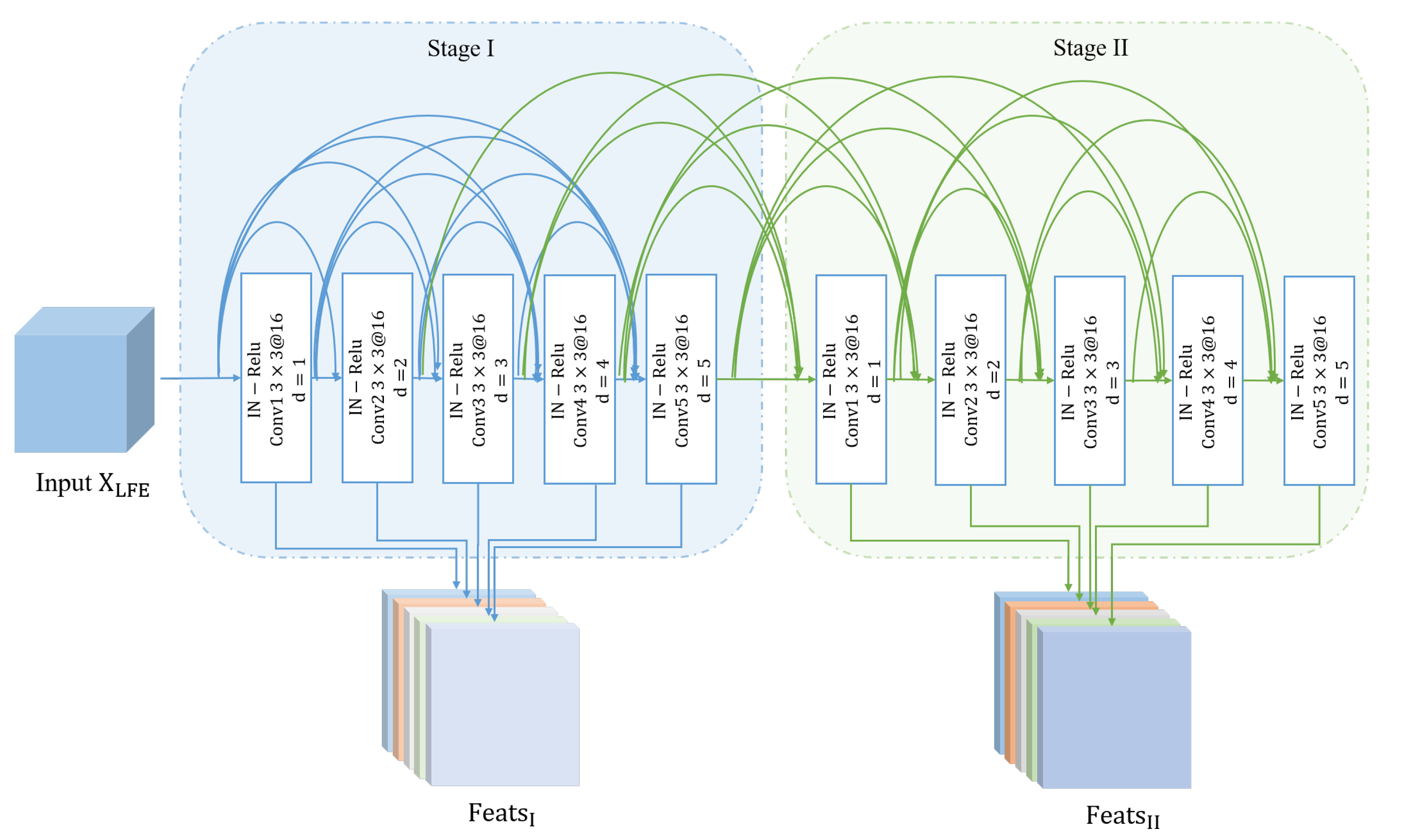
As the backbone of CFF-FCN, LFEB is a two-stage network based on dilated convolutions with dense connections and reverse loop mechanism. The stacking of dilated convolutions with different dilation rates fully considers the local information of different scales. Dense connections ensure the maximum information transmission in the network [31]. Let $X_{LFE}$ be the input of LFEB, which contains five dilated convolutions with convolution kernels of $3\times 3$. The specific architecture is displayed in Figure 4. To ensure the continuity of local information while avoiding gridding effect, we employ a set of incremental dilation rates that set as $d=[1,2,3,4,5]$. The nonlinear transformation $H_d(·)$ of each convolutional layer is composed of instance normalization (IN) [32], rectified linear unit (ReLU) and convolution (Conv).

The network structure of the multi-layer stack yields the deviation of the data distribution. To reduce the impact of the distribution changes, normalization strategy is usually used in neural networks to map the data to a certain interval. Neural networks taking patches as input generally use batch normalization (BN) [33] to normalize data in a whole batch of images. While the batch size of the FCN-based classification network is 1, BN is not applicable. Therefore, we use IN for normalization in the channel dimension. Normalization operation is performed within single sample. The specific operation can be expressed as:

$$\tilde{Z}=\gamma \left(\frac{Z-\mu \left(Z\right)}{\sigma \left(Z\right)}\right)+\beta ,$$

(6)

where $Z\in {\mathbb{R}}^{1\times H\times W\times K}$ represents the tensor to be normalized, K is the number of channels. $\tilde{Z}$ denotes the normalized result. $\gamma$ and $\beta$ are parameters to be learned. $\mu \left(Z\right)$ and $\sigma \left(Z\right)$ represent the mean and variance of Z, which are calculated as follows:

$${\mu }_k\left(Z\right)=\sum _{h=1}^H\sum _{w=1}^W{Z}_{khw},$$

(7)

$${\sigma }_k\left(Z\right)=\sqrt{\frac{1}{HW}\sum _{h=1}^H\sum _{w=1}^W{\left(Z_{khw}-{\mu }_k\left(Z\right)\right)}^2+\epsilon }.$$

(8)

Here, h, w, and k represent the index subscript of the spatial location and the channel dimension, respectively. IN can be seen as an adjustment of global information to ensure fast convergence of networks.

In the first stage (Stage-I), each layer takes the outputs of all previous layers as input, and its output is also directly delivered to all subsequent layers. Let $X_i^I$ be the output of i-th convolutional layer in Stage I, the calculation of LFEB can be represented as:

$$X_i^I=H_i\left(\left[X_{LEF},X_1^I,\dots ,X_{i-1}^I\right]\right).$$

(9)

$[·]$ denotes the cascade operation of features. For each dilated convolutional layer, the corresponding maximum and minimum receptive field can be calculated as:

$${RF}_{max}^i={RF}_{max}^{i-1}+\left(k_i-1\right)·stride,$$

(10)

$${RF}_{min}^i=k_i·stride.$$

(11)

$stride$ is set to 1. Receptive fields cover $3\times 3$ to $31\times 31$ after Stage-I. In Stage-I, each layer is directly connected to the subsequent layers. The network learns and retains richer features by feature reuse at different levels, which enhances the feature transfer from shallow to deep. At the same time, the implementation of multi-scale receptive fields can adaptively capture and fuse semantic information in different scale, which is conducive to retaining local details and obtaining more complex and robust feature maps. The output of each layer is aggregated as the first stage feature of LFEB:

$${Feats}_I{=\parallel }_{i=1}^5{X}_i^I.$$

(12)

$\parallel$ means continuous cascade operation for feature maps.

Inspired by the alternate update clique [33], we introduce the loop mechanism based on parameter reuse into LFEB and further refine ${Feats}_I$ on the basis of the first-stage network, which modulate low-level features with high-level semantic information. The specific unfold of LFEB is shown in Figure 4. The second stage network (Stage-II) uses the latest output results of other layers to update weights of the current layer. The output of Stage-II can be expressed as:

$$X_i^{II}=H_i\left(\left[{\parallel }_{d=1}^{i-1}{X}_d^{II}{,\parallel }_{d=i+1}^5{X}_d^I\right]\right).$$

(13)

In Stage-II, second stage features of all the previous layers and first stage features of all subsequent layers are concatenated to update the current layer. The higher-level semantic information is fed back into low-level layers to refine features of each layer in an alternate update manner.

Table 1. Forword propagation of LEFB.

Input	Weight	Output
$X_{LEF}$	$W_{01}$	$X_1^I$
$[X_{LEF},X_1^I]$	$[W_{02},W_{12}]$	$X_2^I$
$[X_{LEF},X_1^I,X_2^I]$	$[W_{03},W_{13},W_{23}]$	$X_3^I$
$[X_{LEF},X_1^I,X_2^I,X_3^I]$	$[W_{04},W_{14},W_{24},W_{34}]$	$X_4^I$
$[X_{LEF},X_1^I,X_2^I,X_3^I,X_4^I]$	$[W_{05},W_{15},W_{25},W_{35},W_{45}]$	$X_5^I$
$[X_2^I,X_3^I,X_4^I,X_5^I]$	$[W_{21},W_{31},W_{41},W_{51}]$	$X_1^{II}$
$[X_1^{II},X_3^I,X_4^I,X_5^I]$	$[W_{12},W_{32},W_{42},W_{52}]$	$X_2^{II}$
$[X_1^{II},X_2^{II},X_4^I,X_5^I]$	$[W_{13},W_{23},W_{43},W_{53}]$	$X_3^{II}$
$[X_1^{II},X_2^{II},X_3^{II},X_5^I]$	$[W_{14},W_{24},W_{34},W_{54}]$	$X_4^{II}$
$[X_1^{II},X_2^{II},X_3^{II},X_4^{II}]$	$[W_{15},W_{25},W_{35},W_{45}]$	$X_5^{II}$

displays the forward propagation of LEFB. $W_{ij}$ denotes parameters of convolution from $X_i$ to $X_j$. Stage-I can be regarded as a layer-by-layer initialization process. After Stage-II, any layer has two-way connections to other layers. The update layer receives the most advanced feedback information.It realizes top-down refinement. The feedback structure maximizes communication between all layers. Outputs of all layers in Stage-II are connected as the second feature of LFEB:

$${Feats}_{II}{=\parallel }_{i=1}^5{X}_i^{II}.$$

(14)

Forward propagation networks usually employ the highest-level semantic features as the classification feature. In fact, fine-grained features captured by low-level layers can provide more structural information for classification. In order to take full advantage of different levels of features, we deliver ${Feats}_I$ into CFFB to extract global class information, which is aggregated with ${Feats}_{II}$ to generate the final classification feature.

3.2. Class Feature Fusion Block

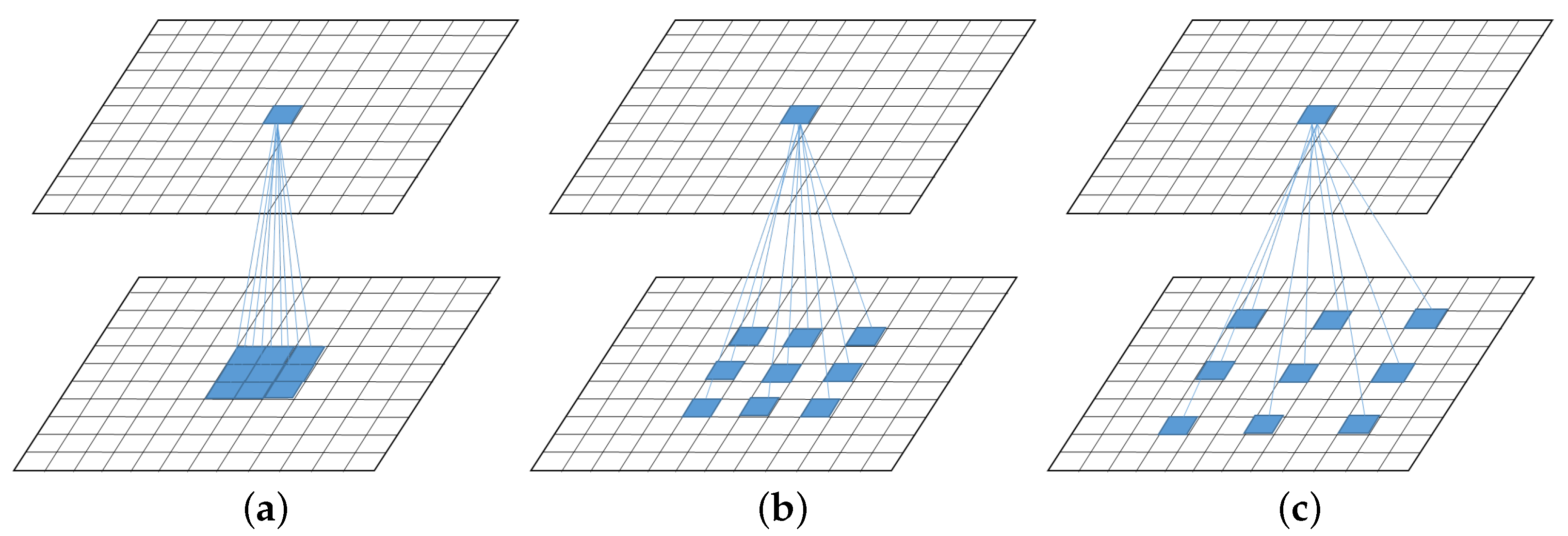
Non-local neural networks explore the similarity relationship between all pixels and update pixel features with global information. Taking into account the characteristics of HSIs, the pixel-by-pixel global information not only contains a large amount of highly correlated redundant information, but also brings high calculation cost. In response to this problem, we design CFFB to reconstruct pixel information by more representative global class context features, which reduces the computational cost while improving the discrimination of pixel features. The specific structure is shown in Figure 5, which mainly includes two parts: class feature extraction and pixel feature fusion.

The most intuitive way to obtain the class representation in HSI is to take the average of all pixel features of the current category as the class center. In actual classification, the labels of all pixels is not available in advance. To this end, we employ a coarse classification mechanism to classify by the intermediate features and obtain the class probability of each pixel in a supervised manner. Through the weighted average of the pixel features and the corresponding class probability, the approximate class center is obtained as the class representation. Let the input of CFFB be $X_{CFR}\in {\mathbb{R}}^{N\times H\times W\times L}$, where L is the number of input channels. The class probabilities of pixels on the spatial position $i(1\le i\le HW)$ is calculated as follows:

$$p_i=softmax\left(f_{cls}\left(x_i\right)\right).$$

(15)

$x_i$ represents the input feature of pixel i. $f_{cls}$ denotes the classifier that maps the input from ${\mathbb{R}}^{K_0}$ to ${\mathbb{R}}^C$. The class representation of the c-th class can be defined by the weighted average with features of all pixels and their probability belonging to the c-th class:

$$F_c=\frac{{\Sigma }_{i=1}^{HW}{p}_i^c{f}_p\left(x_i\right)}{{\sum }_{i=1}^{HW}{p}_i^c},$$

(16)

where $p_i^c$ is the c-th element of $p_i$, and $f_p$ aims to calculate the pixel feature. $f_{cls}=W_{cls}{x}_i$ and $f_p=W_p{x}_i$ are implemented by $1\times 1$ convolution. If the coarse classification result shows that the pixel belongs to the c-th class, the pixel has the largest contribution to the c-th class representation. Class features allow the network to capture the overall representation of each class from a global view. Coarse classification provides powerful supervision information in training phase to learn more discriminative features of each class.

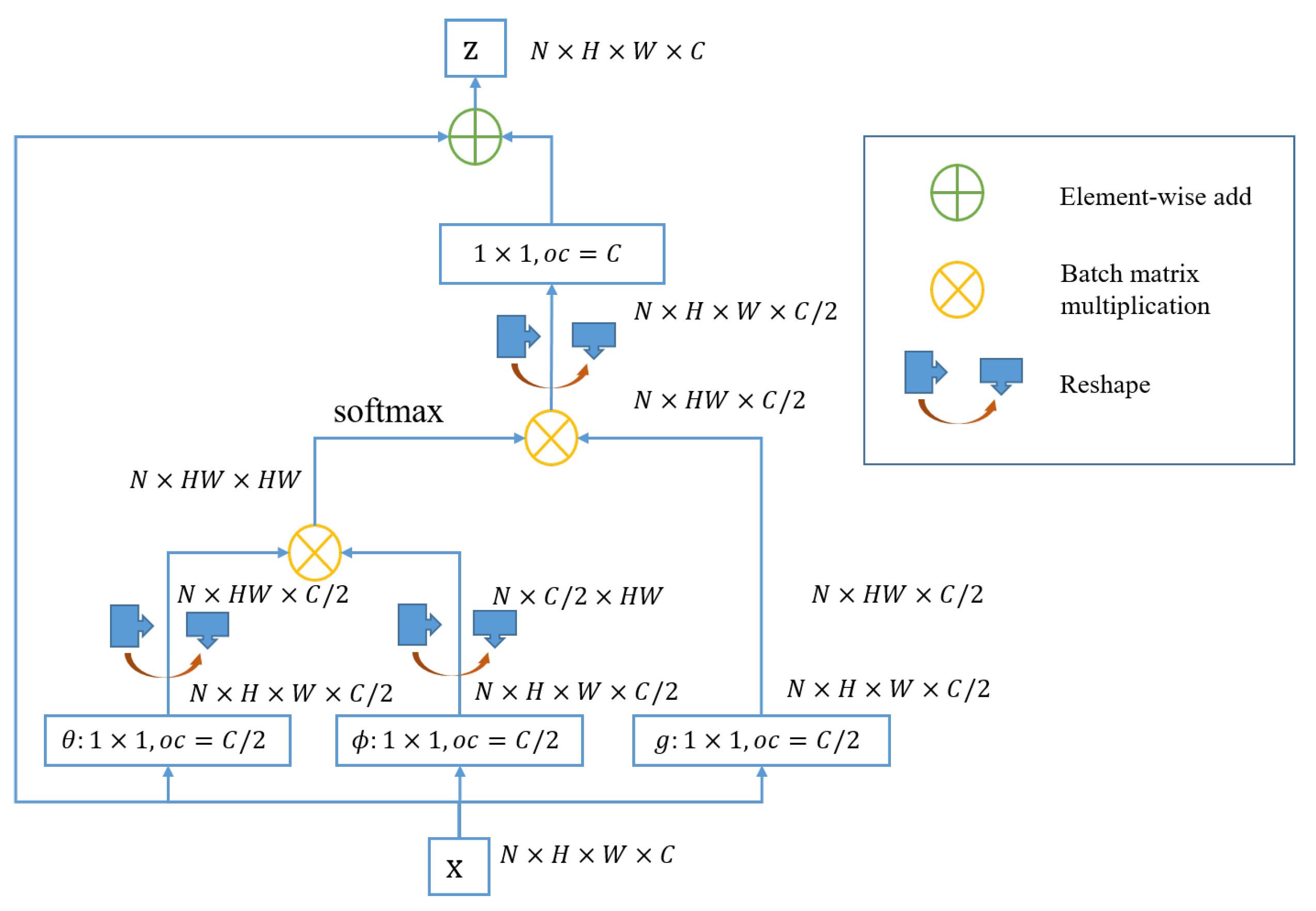
Pixel feature fusion aims to learn relations between pixels and class representations, and exploit global class context information to enhance the features of each pixel. We utilize the relationship estimation method of non-local block and calculate relations between each pixel and each class (affinity matrix):

$$A_{ic}=e^{\theta {\left(x_i\right)}^T\varphi \left(F_c\right)},$$

(17)

where $A\in {\mathbb{R}}^{HW\times C}$ is affinity matrix, and $A_{i}c$ is an element of A that indicates the contribution degree of the class feature $F_c$ to the reconstructed pixel i. $\theta \left(x_i\right)=W_{\theta }{x}_i$ and $\varphi \left(F_c\right)=W_{\varphi }{F}_c$ are $1\times 1$ convolutions. The global estimation of the pixel i can be expressed as:

$$y_i=\frac{{\sum }_{c=1}^C{A}_{ic}g\left(F_c\right)}{{\sum }_{c=1}^C{A}_{ic}},$$

(18)

$g\left(F_c\right)=W_g{F}_c$ is a class feature transform function implemented by $1\times 1$ convolution. Therefore, the output of CFFB can be described as:

$$Y_{CFR}=softmax\left(X_{CFR}^T{W}_{\theta }^T{W}_{\varphi }\mathrm{F}\right)\left(F^T{W}_g^T\right).$$

(19)

The global class representation learned in a supervised manner is obtained from highly correlated pixel features of the same category. The process of coarse classification can be seen as clustering of pixels, which can adaptively gather semantically related pixels and enlarge the differences between classes. Pixel feature mapping by category features and similarity matrix allow the network to re-estimate pixel features with key semantic information, which reduces intra-class differences and comprehensively improve the discrimination of fusion features.

Finally, we concatenate fusion features with second-stage features of the backbone network to obtain the final classification feature $[{Feats}_{II},Y_{CFR}]$ that is sent to the classification layer. Due to existing unlabeled samples in hyperspectral images, we only calculate the loss function for labeled training samples. In this paper, cross entropy loss is used for coarse classification and final classification. The cross entropy loss is described as:

$${\mathcal{L}}_{\mathrm{softmax}}=-\sum _{i=1}^m{t}_i^{c}log{p}_i^c,$$

(20)

where m is the total number of training samples, $t_i^c$ is the c-th value of a label vector for pixel i, and $p_i^c$ is the the corresponding probability. The loss function of CFF-FCN can be written as:

$${\mathcal{L}}_{CFR}={\mathcal{L}}_{final}+\lambda L_{coarse}.$$

(21)

$\lambda$ is the weight factors to balance the two loss functions.

4. Experimental Results

4.1. Experimental Data Sets

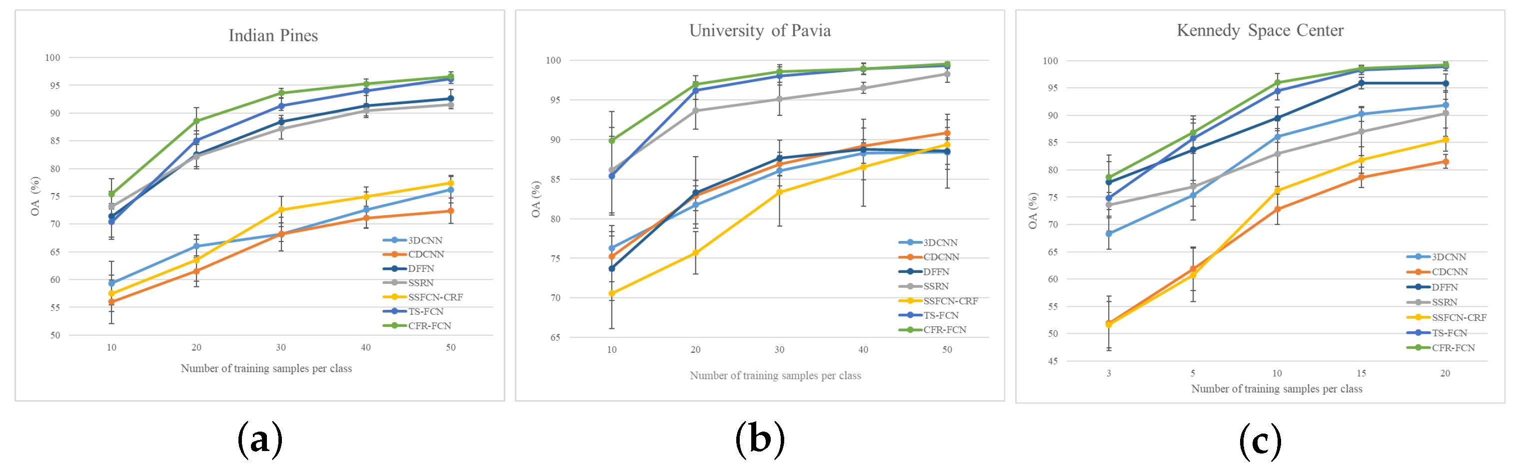
To evaluate the performance of the proposed method, we conducted experiments and analyses on three widely used public data sets, including Indian Pines (IP), University of Pavia (UP), and Kennedy Space Center (KSC). The details of these three data sets are described as follows.

Table 2. The samples for each category of IP, UP, and KSC.

	IP		UP		KSC
	Class	Total	Class	Total	Class	Total
1	Alfalfa	54	Asphalt	6631	Scrub	716
2	No-till corn	1434	Meadow	18,649	Willow swamp	243
3	Min. till corn	834	Gravel	2099	CP hammock	256
4	Corn	234	Trees	3064	CP/Oak hammock	252
5	Pasture grass	497	Metal sheets	1345	Slash pine	161
6	Grass-trees	747	Bare soil	5029	Oak/Broadleaf hammock	229
7	Grass-pasture-mowed	26	Bitumen	1330	Hardwood swamp	105
8	Hay-windrowed	489	Bricks	3682	Graminoid marsh	431
9	Oats	19	Shadows	947	Spartina marsh	520
10	No-till soybean	968			Cattail marsh	404
11	Min. till soybean	2468			Salt marsh	419
12	Clean till soybean	614			Mud flats	503
13	Wheat	212			Water	927
14	Woods	1294
15	Buildings–grass–trees	380
16	Woods	95
		10,366		42,776		5211

lists category names and the number of corresponding labeled samples.

IP data sets were the earliest test data used for HSI classification. They were collected by the Airborne Visible Infrared Imaging Spectrometer (AVIRIS) in Northwest Indiana, USA. A subset of the whole data set with a size of $145\times 145$ is cut and annotated for HSI classification. The wavelength range is 0.4–2.5 μm, including 224 reflection bands. After removing the noise and water absorption bands, the remaining 200 bands are used as research objects. The spatial resolution is about 20 m, which is easy to produce mixed pixels and brings difficulty to classification. The IP data set includes 16 classes of ground truth. Moreover, 9 categories with labeled samples larger than 400 were selected for the experiment.

The UP data set was collected by the Reflective Optics System Imaging Spectrometer (ROSIS) from the University of Pavia, Italy. It contains 115 bands in the wavelength range of 0.43–0.86 μm, with a spatial resolution of $1.3$ m. Moreover, 12 bands were eliminated due to the influence of noise. The size of UP was $610\times 340$, covering 9 classes, including trees, asphalt roads, bricks, pastures, etc.

The KSC data set was acquire by the AVIRIS at the Kennedy Space Center in Florida, USA. The image contains data of 224 bands from 0.4–2.5 μm, with a spatial resolution of 18 m. After removing the water absorption and noise bands, the remaining 176 bands were used for experiments. KSC contains $512\times 614$ pixels and 13 land cover types.

The experimental results including Figure S1 and Table S1 of the Bostwana data set can be found in the Supplementary Materials.

4.2. Experimental Setup

Each data set was divided into a training set, validation set, and test set. The training set was served for back propagation to optimize model parameters. The validation set did not participate in the training, but evaluated the temporary model in the training phase. The test set evaluated the classification ability of the final model. For IP and UP data sets, 30 labeled samples of each class were randomly selected for training and validation. The remaining labeled samples were used for testing. For the KSC data set, 10 labeled samples for each class were randomly selected for training and verification.

We adopted class-based accuracy, overall accuracy (OA), average accuracy (AA), and kappa coefficient to the evaluation classification performance. The experiment was implemented on the PyTorch framework. The hardware platform included an Intel E5-2650 CPU, an NVIDIA GTX2080Ti GPU. The number of training iterations was 1000, and the learning rate was 0.0003.

We compared the proposed CFF-FCN with several state-of-the-art deep learning-based classifiers, including 3D-CNN [34], the contextual deep CNN (CDCNN) [35], the deep feature fusion network (DFFN) [36], the spectral–spatial residual network (SSRN) [37], and the spectral–spatial fully convolutional network (SSFCN-CRF) [22]. These methods all employ spectral–spatial features to implement HSI classification. Among them, 3D-CNN, CDCNN, DFFN, and SSRN are patch-based CNNs, and SSFCN-CRF is an image-based fully convolutional framework. The network settings of the above methods follow the corresponding references. Meanwhile, we also conducted experiments on two-stage networks (TSFCN) without CFFB, which can be regarded as the backbone of our proposed CFF-FCN. The specific numerical results and full classification maps are listed in

Table 3. Classification accuracy(%) for Indian Pines using different classifiers.

CLASS	3DCNN	CDCNN	DFFN	SSRN	SSFCN-CRF	TSFCN	CFF-FCN
2	51.03	57.02	81.81	78.33	56.94	82.3	88.09
3	55.44	50.11	90.0	90.14	59.75	93.71	95.68
5	85.78	87.56	93.23	95.48	83.51	96.72	97.6
6	94.16	90.66	93.6	99.12	94.03	99.3	99.65
8	98.56	98.06	99.13	99.89	98.8	100	99.96
10	54.22	55.66	86.64	85.36	72.77	90.15	91.25
11	63.65	61.92	83.59	78.24	63.65	86.38	89.79
12	47.71	51.54	93.89	88.94	66.18	92.45	94.61
14	91.6	90.5	94.28	98.53	92.54	99.86	99.91
OA	68.18	68.2	88.42	87.19	72.6	91.3	93.61
AA	71.35	71.45	90.69	90.45	76.46	93.43	95.17
$\kappa \times 100$	62.68	62.91	86.48	85.05	68.16	89.83	92.53

,

Table 4. Classification accuracy(%) for University of Pavia using different classifiers.

CLASS	3DCNN	CDCNN	DFFN	SSRN	SSFCN-CRF	TSFCN	CFF-FCN
1	83.53	83.12	79.0	95.95	77.76	96.99	98.04
2	91.45	91.58	89.94	94.68	81.57	97.29	97.94
3	84.98	79.55	89.04	94.56	78.57	98.19	98.34
4	89.18	94.58	86.53	95.84	88.6	99.11	99.05
5	99.57	99.93	97.35	100	96.83	99.99	100
6	58.22	74.39	84.35	97.79	87.21	99.48	99.13
7	84.3	87.22	93.92	99.27	87.94	99.92	99.95
8	91.91	76.73	90.09	87.97	85.99	99	99.42
9	99.17	99.5	89.59	98.14	96.37	99.79	99.91
OA	86.07	86.9	87.65	95.12	83.36	98.04	98.49
AA	86.92	87.4	88.87	96.02	86.76	98.86	99.09
$\kappa \times 100$	81.51	82.74	83.85	93.6	78.62	97.42	98.01

and

Table 5. Classification accuracy(%) for Kennedy Space Center using different classifiers.

CLASS	3DCNN	CDCNN	DFFN	SSRN	SSFCN-CRF	TSFCN	CFF-FCN
1	91.97	92.56	94.5	94.27	82.36	98.99	98.38
2	81.55	60	69.87	87.42	67.38	91.5	93.99
3	91.71	73.17	87.85	67.4	88.21	96.59	96.5
4	51.65	23.39	71.45	26.69	54.42	63.6	73.43
5	66.89	55.36	84.77	71.32	53.71	74.44	88.48
6	62.01	57.58	84.89	36.71	66.21	95.48	97.21
7	94.21	87.68	99.89	74.32	96.21	100	100
8	77.48	70.86	67.77	79.41	47.65	92	93.54
9	89.73	93.69	90.8	78.47	79.2	96.94	97.49
10	83.83	51.29	90.05	84.06	53.32	95.69	95.63
11	98.7	94.08	99.41	98.41	87.53	100	100
12	81.58	37	92.05	86.92	69.47	91.05	95.17
13	97.74	85.97	99.65	99.96	100	100	100
OA	86.08	72.78	89.5	82.94	76.24	94.43	95.99
AA	82.23	67.89	87.15	75.8	72.74	92.02	94.6
$\kappa \times 100$	84.5	69.65	88.3	80.93	73.54	93.79	95.53

and Figure 6, Figure 7 and Figure 8.

4.3. Classification Maps and Categorized Results

4.3.1. Indian Pines

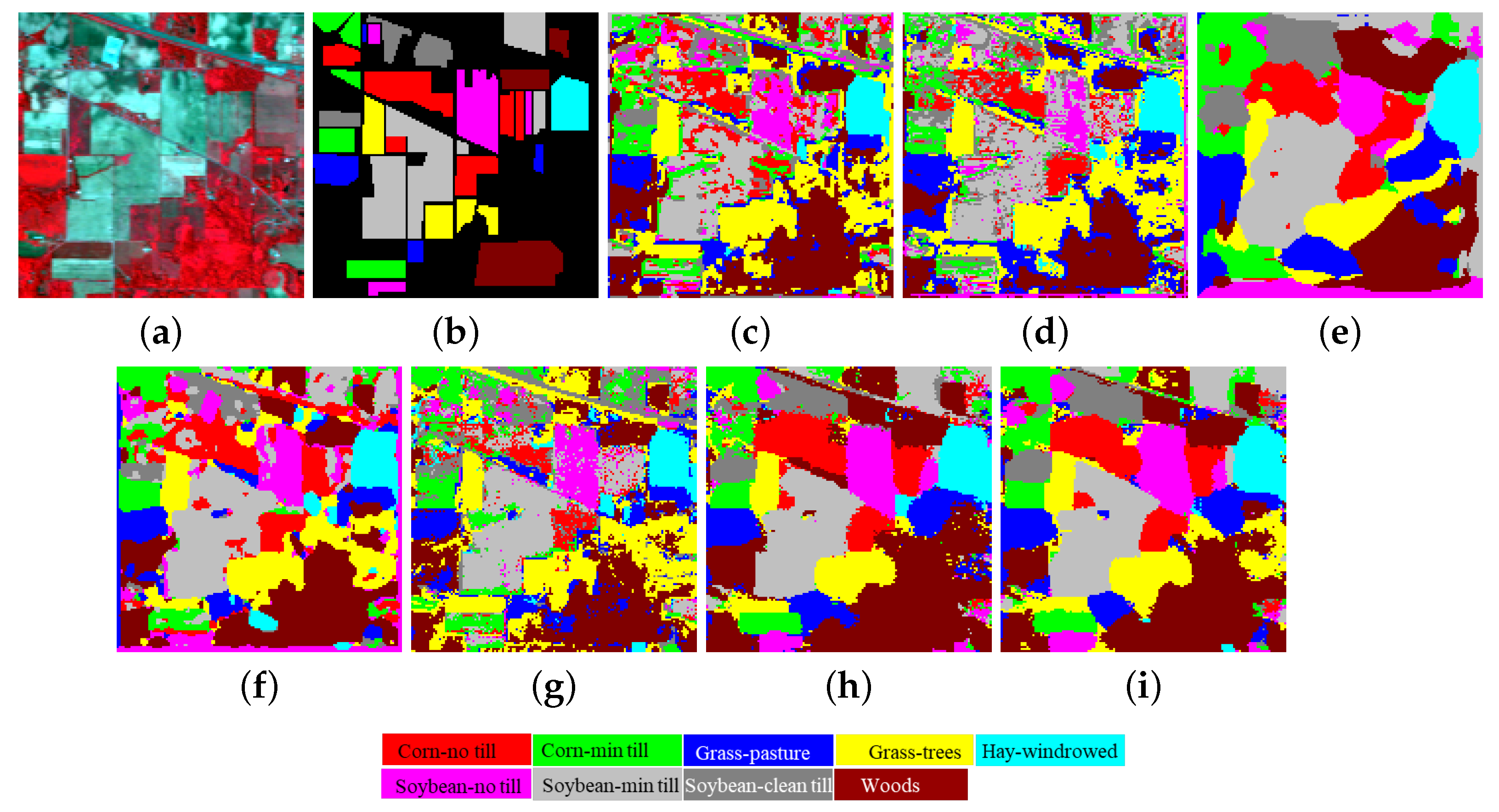
Figure 6 and Table 3 respectively show the classification maps and numerical results of different methods in the IP data set. The TSFCN and CFF-FCN proposed in this paper are significantly better than other methods in three overall indicators. TSFCN achieves 100% classification accuracy on class 8 (Hay-windrowed), and CFF-FCN maintains the best accuracy on other classes. The introduction of global class context information makes OA increase by 2.31%. Due to the limitation of the number of training samples, 3DCNN, CDCNN and SSFCN-CRF cannot extract reliable spectral–spatial features, and the classification performance is relatively weak. Classification accuracies of DFFN and SSRN is preceded only to the proposed methods. Figure 6c,d,f also indicate that 3DCNN, CDCNN, and SSFCN-CRF have obvious class mixing and salt and pepper noise. Classification map of DFFN is smoother than SSRN’s. However, DFFN seems to have a certain degree of overfitting. The classification maps of TSFCN and CFF-FCN show the best visual effects, especially the use of global information makes the category edges of CFF-FCN smoother.

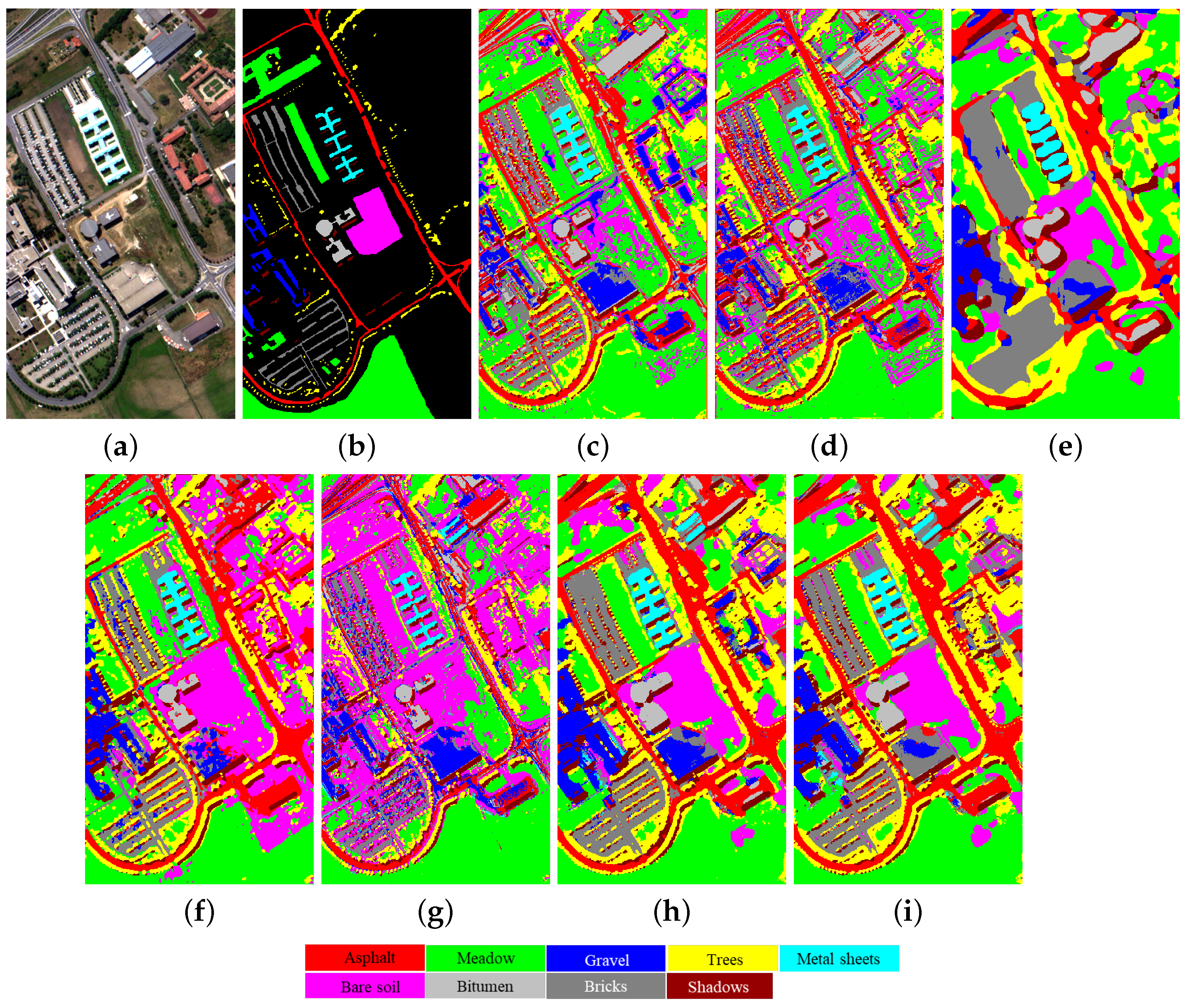
4.3.2. University of Pavia

Table 4 reports the classification accuracies for the UP data set. CFF-FCN shows the best performance in most categories and overall indexes. CFF-FCN and SSRN have achieved 100% class accuracy in class 5 (metal sheets). Compared with TSFCN, the OA of CFF-FCN is increased by 0.45%, indicating the effectiveness of CFFB. Figure 7 display the classification map of different methods. The 3DCNN, CDCNN, and SSFCN-CRF all have large regions of misclassification, and the class edges are not smooth. DFFN can observe obvious overfitting phenomenon in the UP data set. Compared with other methods, classification maps of TSFCN and CFF-FCN obviously have fewer misclassification points, and the class boundaries are clearer and smoother. Comparing TSFCN and CFF-FCN, it can be observed that global class information can alleviate the confusion of category boundaries to a certain extent.

4.3.3. Kennedy Space Center

Table 5 and Figure 8 present the experimental results of different methods on the KSC data set. Table 5 indicates that the performance of our proposed TSFCN and CFF-FCN is significantly better than other methods, achieving 100% classification accuracies for classes 7, 11, and 13. Compared with TSFCN, the OA of CFF-FCN increases by 1.56%. The classification accuracy of DFFN is second only to the proposed TSFCN and CFF-FCN. Table 5 shows that class 4 (CP) and class 6 (Oak) are difficult to distinguish correctly. Compared with other classifiers, CFF-FCN has achieved better accuracy in these two categories. From Figure 8b, it can be seen that the labeled samples of KSC only occupy a very small part of the entire image and are loosely distributed. In the classification map of CDCNN, there exists a lot of salt and pepper noise. DFFN still exhibits overfitting. SSFCN-CRF can detect all objects on the water surface. However, its classification map does not have clear category boundaries. Figure 8h also shows that the classification map of CFF-FCN is closer to the ground-truth map.

5. Discussion

In this section, we further discuss several factors affecting the performance of CFF-FCN. First, different numbers of training samples are input into the network to evaluate the performance in the case of limited numbers of training samples. Second, the effect of loss balance parameter $\lambda$ with different values on classification results. Third, the effect of reverse loop mechanism and classification feature fusion module on classification accuracy is studied in an ablation manner. Finally, we compare and analyze the running times and the numbers of network parameters to evaluate the running efficiencies of different methods.

5.1. Investigation of the Proportion of Training Samples

Figure 9 shows the OAs and their standard deviations of different methods under different numbers of training samples. The number of training samples for the IP and UP data sets varies from 10 to 50. Due to the KSC label sample limitation, the number of training samples ranges from 3 to 20. In the case of precious few training samples, CDCNN and SSFCN-CRF are unable to provide reliable classification results on the three data sets. SSRN with higher model complexity can obtain relatively better classification performances in most cases. Figure 9c indicates that when the number of training samples on KSC is greater than 10, the classification performance of SSRN is not as good as 3DCNN. DFFN achieved competitive classification performances on both IP and KSC data sets. Of the three data sets, the OAs provided by TSFCN and CFF-FCN is better than other algorithms. In particular, in the case of fewer training samples, CFF-FCN can obtain a more reliable classification effect than TSFCN, reflecting the effectiveness of CFFB and the robustness of CFF-FCN. The standard deviation reflects the stability of the network performance. With the three data sets, the stability of TSFCN and CFF-FCN is better than other methods. Especially with the increase of training samples, the proposed models become more stable.

5.2. Investigation of $\lambda$

$\lambda$ is the weighting factor used to balance the final classification loss $L_{final}$ and the coarse classification loss $L_{coarse}$ in Equation (21). To study the influence of $\lambda$ on the classification performance of CFF-FCN, we conducted experiments with different values of $\lambda$ on three data sets, and the results are reported in Figure 10. It can be seen that CFF-FCN on the IP data set is most sensitive to changes in $\lambda$. For IP and KSC data sets, the model performances are best when $\lambda$ is 1. The UP data set is the least sensitive to changes in $\lambda$, and OA changes very little under different $\lambda$. Combining the classification results of the three data sets, we set $\lambda$ to 1.

5.3. Ablation Study

The ablation experiments in this section mainly discuss three issues: (1) the effectiveness of CFFB; (2) the effectiveness of the second stage of LFEB; (3) the contributions of ${Feats}_I$ and ${Feats}_{II}$ to HSI classification. To this end, we conducted experiments on six types of networks according to different settings, and named them Model 1–6, among which Model 2 and Model 5 correspond to the TSFCN and CFF-FCN mentioned above. The specific model settings and classification accuracy are shown in

Table 6. Effectiveness analysis (OA%) of CRFB and LFEB.

Models	CFFB	Stage-II	Input of CFFB		Output of LFEB		Data Sets
			${\mathit{F}\mathit{e}\mathit{a}\mathit{t}\mathit{s}}_{\mathit{I}}$	${\mathit{F}\mathit{e}\mathit{a}\mathit{t}\mathit{s}}_{\mathit{I}\mathit{I}}$	${\mathit{F}\mathit{e}\mathit{a}\mathit{t}\mathit{s}}_{\mathbf{I}}$	${\mathit{F}\mathit{e}\mathit{a}\mathit{t}\mathit{s}}_{\mathit{II}}$	IP	UP	KSC
1	×	×	×	×	✓	×	89.4	97.73	94.47
2	×	✓	×	×	×	✓	91.3	98.04	94.43
3	×	✓	×	×	✓	×	90.43	98.45	94.85
4	✓	×	✓	×	✓	×	90.79	98.15	95.01
5	✓	✓	✓	×	×	✓	93.61	98.6	95.99
6	✓	✓	×	✓	×	✓	92.82	98.5	95.82

.

Models 1–3 do not employ CFFB module. When LFEB does not reuse the second-stage parameters, the classification accuracies of Model 1 on IP and UP are significantly lower than that of Model 2 and 3. It demonstrates that the further refinement of the features from top to bottom in the second stage is conducive to improve the representation ability of the network. The similar conclusion can be drawn from Models 4–6. Comparing Model 2 and Model 3, it can be found that although ${Feats}_{II}$ is a higher-level feature, ${Feats}_I$ shows stronger classification ability on UP and KSC. Parameters reused in Stage-II are also involved in calculation of ${Feats}_I$. In Stage-II, high-level features are fed back to modulate low-level information, and ${Feats}_I$ is also refined to present the classification ability different from ${Feats}_{II}$. In order to increase feature complexity and discrimination, we use ${Feats}_I$ as the input of CFFB to reconstruct pixel features. The comparison of the results of Models 5 and 6 also show that the joint features at different stages can indeed improve the representation ability of the network and obtain more accurate classification results.

5.4. Investigation of Running Efficiency

Table 7. Comparison of running efficiency between different methods.

Models	Training Time(s)			Testing Time(s)			Parameters(M)
	IP	UP	KSC	IP	UP	KSC
3DCNN	155.85	154.39	79.30	1.47	6.67	0.83	0.2
CDCNN	179.25	177.49	104.75	1.48	6.84	0.84	1.06
DFFN	784.10	957.53	548.50	38.08	225.63	22.60	0.4
SSRN	226.64	169.16	103.49	4.90	22.51	2.73	0.36
SSFCN-CRF	25.65	114.04	282.17	0.01	0.02	0.02	0.11
TSFCN	76.15	159.62	294.71	0.02	0.08	0.17	0.12
CFF-FCN	102.78	186.51	310.29	0.02	0.08	0.16	0.12

displays training times, testing times and numbers of network parameters for different methods. Among them, training times and test times correspond to the experimental settings in Table 3, Table 4 and Table 5, and network parameters are counted based on the IP data set. For patch-based methods, training times, and testing times are proportional to the number of samples, since they are pixel-by-pixel processing methods. For FCN-based methods, training times and testing times are proportional to the image size, because they need to traverse the entire image in each epoch. For the IP data set, patch-based methods require longer training times, and the training efficiency is not as good as image-based classification methods. For the UP data set, patch-based methods except DFFN and image-based methods have little difference in training time. For data sets with few labeled samples and large image size, the training time of FCNs is generally longer than that of patch-based methods. In the test phase, FCNs only need to traverse the image once, so the test time is generally shorter than patch-based methods. DFFN is a deeper classification network based on residual connections, resulting in the longest time in both the training and testing phases. In addition, compared with the SSRN whose classification performance is closest to CFF-FCN, our parameter amount is only 1/3 of SSRN. In practical applications, CFF-FCN can balance running efficiency and classification accuracy.

6. Conclusions

In this study, we propose a novel deep learning framework (CFF-FCN) with LEFB and CFFB to acquire the local spatial information and global class context for HSI classification. By dilated convolutions and reverse loop mechanism, LEFB provides multi-level semantic information covering different receptive fields. CFFB clustering correlated pixels, by supervised information, captures the global class representation and reconstructs pixel feature with class context. CFFB, different from pixel-by-pixel non-local extraction, replaces redundant pixel information with more representative class features in the reconstruction process, which decreases the demand for computing resources. Local spatial information and global reconstructed features are aggregated to implement classification. Extensive experiments and ablation study over three HSI data sets demonstrate that the proposed method provides promising classification performance compared with several state-of-the art deep learning methods. However, there are some hard samples at the boundaries between different classes that are always misclassified. How to further solve this problem will be the focus of our follow-up research.