Article

Assessment and Attribution of Mangrove Forest Changes in the Indian Sundarbans from 2000 to 2020

1
School of Oceanographic Studies, Jadavpur University, 188 Raja S. C. Mullick Road, Kolkata 700032, India
2
UCL Coastal and Estuarine Research Unit, University College London, London WC1E 6BT, UK
3
Tyndall Centre for Climate Change Research, University of East Anglia, Norwich NR4 7TJ, UK
*
Author to whom correspondence should be addressed.
Remote Sens. 2021, 13(24), 4957; https://doi.org/10.3390/rs13244957
Submission received: 13 October 2021 / Revised: 20 November 2021 / Accepted: 25 November 2021 / Published: 7 December 2021
(This article belongs to the Section Forest Remote Sensing)

Abstract

:
The Indian Sundarbans, together with Bangladesh, comprise the largest mangrove forest in the world. Reclamation of the mangroves in this region ceased in the 1930s. However, they are still subject to adverse environmental influences, such as sediment starvation due to migration of the main river channels in the Ganges–Brahmaputra delta over the last few centuries, cyclone landfall, wave action from the Bay of Bengal—changing hydrology due to upstream water diversion—and the pervasive effects of relative sea-level rise. This study builds on earlier work to assess changes from 2000 to 2020 in mangrove extent, genus composition, and mangrove ‘health’ indicators, using various vegetation indices derived from Landsat and MODIS satellite imagery by performing maximum likelihood supervised classification. We show that about 110 km2 of mangroves disappeared within the reserve forest due to erosion, and 81 km2 were gained within the inhabited part of Sundarbans Biosphere Reserve (SBR) through plantation and regeneration. The gains are all outside the contiguous mangroves. However, they partially compensate for the losses of the contiguous mangroves in terms of carbon. Genus composition, analyzed by amalgamating data from published literature and ground-truthing surveys, shows change towards more salt-tolerant genus accompanied by a reduction in the prevalence of freshwater-loving Heiritiera, Nypa, and Sonneratia assemblages. Health indicators, such as the enhanced vegetation index (EVI) and normalized differential vegetation index (NDVI), show a monotonic trend of deterioration over the last two decades, which is more pronounced in the sea-facing parts of the mangrove forests. An increase in salinity, a temperature rise, and rainfall reduction in the pre-monsoon and the post-monsoon periods appear to have led to such degradation. Collectively, these results show a decline in mangrove area and health, which poses an existential threat to the Indian Sundarbans in the long term, especially under scenarios of climate change and sea-level rise. Given its unique values, the policy process should acknowledge and address these threats.

1. Introduction

Mangrove forests are amongst the most productive ecosystems on earth and encompass 136,000 km2 of the sub-tropical and tropical coastal zones [1,2]. Mangroves provide a wide range of ecosystem services [3,4], are vital habitats for terrestrial and marine species [5], and exchange sediment and nutrients with other coastal and estuarine ecosystems [6,7]. From a hazard management perspective, mangroves are also highly valued for their role in attenuating the damaging effects of extreme waves and storm surge water levels [8,9,10]. More recently, mangroves have been shown to act as a globally significant sink for carbon [11,12], to the extent that their conservation and restoration have become important in the context of the global effort to mitigate the impact of climate change [13].
Despite their importance, reclamation (especially for aquaculture), urban development, and coastal landfill have been major aspects driving mangrove loss in the 20th century [14,15]. Up to 35% of the remaining mangrove has been lost over the last 50 years [16]. More recent changes in mangrove forest areas have been mapped at high resolution using remotely sensed data [1], and the current rate of global loss has been estimated at between 0.3 and 0.7% yr−1 [17]. Between 2000 and 2016, land-use change accounted for over 60% of mangrove loss [18], although the rate of direct anthropogenic loss appears to be declining, partly due to an increasing emphasis on mangrove conservation.
In addition to direct anthropogenically driven degradation and loss, mangroves are also sensitive to climate variability and change. Shoreline erosion has accounted for approximately 27% of mangrove loss globally since 2000 [18], with extreme weather events accounting for 11% of the loss. The effects of both climate warming and sea-level rise are already evident through the expansion of mangrove at the expense of saltmarsh [15]. This may offset erosional losses and may enhance terrestrial carbon storage on account of the high belowground carbon storage in mangrove forests [19], although any acceleration in the rate of mangrove loss will counter this effect.
In addition to the mapping of changes in mangrove forest areas [17,18], remotely sensed data have been used in conjunction with ground observations to derive higher-level metrics that can provide a more complete picture of overall mangrove ecosystem health. Mangroves exhibit a high degree of ecological stability and resilience to external perturbations [20], but they are also sensitive to changes in tidal inundation, salinity, and soil chemistry [21]. Although there is no single definition of ‘mangrove health’, relevant measures include tree height [22,23], aboveground biomass and carbon [24,25], and degree of mangrove fragmentation [26]. Discrimination of biophysical parameters using remote sensing data remains challenging, since the spectral responses of mangroves are confounded with background reflectance from a ground surface that varies in sediment type, moisture content, and salinity [27].
Optical remote sensing studies have used characteristics of the vegetation canopy to derive surrogate indices that correlate with more fundamental properties of interest, such as biomass [21]. Most vegetation indices are based on spectral responses in visible, red and near-infrared (NIR) regions of the electromagnetic spectrum [28]. The normalized difference vegetation index (NDVI) has been widely used as a proxy of vegetation productivity and, by implication, overall mangrove forest health [29]. NDVI tends to saturate at high canopy densities [30] and alternatives include the enhanced vegetation index (EVI), which compensates for soil background and atmospheric effects and performs better for denser vegetation cover [31]; the green normalized vegetation index (gNDVI) [32]; and the normalized difference water index (NDWI) [33]. Other supporting measures and derived data products used in regional-scale assessments of mangrove health include percent tree cover (PTC), leaf area index (LAI), and net primary productivity (NPP) [34].
Studies on the identification of stressors and their effects on mangrove health are comparatively limited and recent. This is particularly the case for the globally significant Sundarbans region, where changes in the mangrove forest extent and health appear to be significant. Rahman et al. [35] identified a range of anthropogenic and natural factors for mangrove degradation in the Bangladesh Sundarbans. Paul et al. [36] analyzed drivers of mangrove degradation in the southwestern part of Indian Sundarbans, identifying seven major factors: human uses of mangroves, fishery development, hypersalinity, sediment deposition, storm effects, land erosion, and problems with mangrove regeneration. Despite the obvious potential of multi-spectral remote sensing to provide insights into the health of the mangrove forests, previous applications of remote sensing to the Sundarbans mangroves have mostly focused on detecting land cover changes, feature characterization, and mapping [37,38,39,40,41,42,43].
This paper assesses the changes in both the quantity (extent) and quality (or health) of the mangroves in the Indian Sundarbans mangrove forest from 2000 to 2020, using remotely sensed data. It builds on and extends earlier studies, especially concerning the analysis of various proxy indicators of mangrove health. Within this overall aim, the specific objectives are as follows:
(1)
To detect changes in mangrove forest area, genus composition, and indicators of health across the Indian Sundarbans at various temporal and spatial scales, using Landsat and MODIS satellite imagery.
(2)
To assess the possible drivers of the observed mangrove dynamics, including legacy drivers (e.g., decline in sediment supply and river flow), contemporary progressive drivers (e.g., relative sea-level rise), and shocks (e.g., cyclone landfall).
The analysis presented in this paper supports evidence-based management of the Indian Sundarbans and may be suitable for application elsewhere. It also provides a methodological contribution to the evaluation of changes in mangrove health and how these relate to changes in a range of possible drivers, including climate change and sea-level rise.

2. Materials and Methods

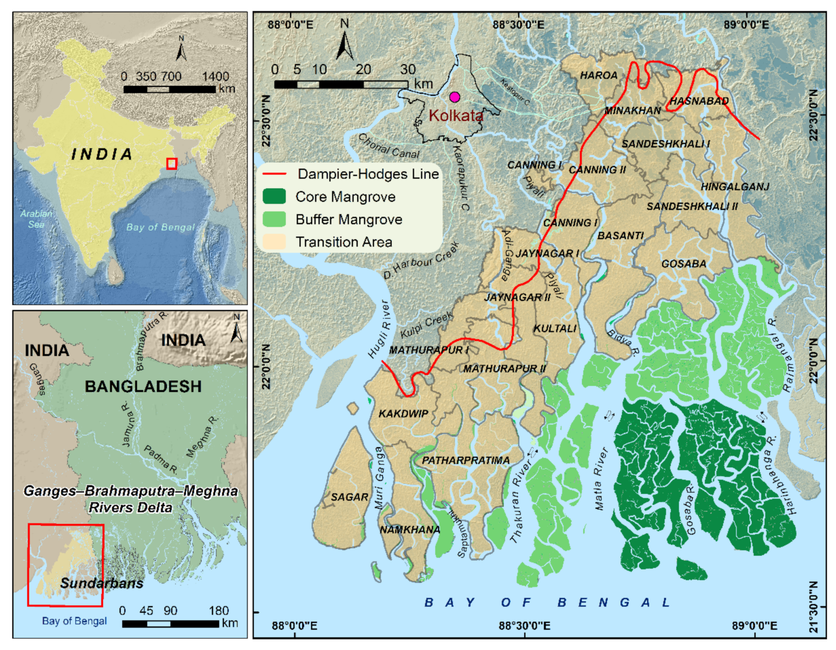
2.1. The Sundarban Biosphere Reserve, India

The Sundarbans (spatial extent: 21°32′ to 22°40′N and 88°05′ to 89°51′E) covers an area of approximately 10,000 km2. A proportion of 62% lies within Bangladesh and 38% lies in India [44], and it comprises the largest contiguous mangrove forest on earth. The depositional environment has evolved with the formation and evolution of the Ganges–Brahmaputra River delta over the last 11,000 years [45]. It consists of a network of mudflats and islands, separated by channels, and created by accumulated sediment loads that these rivers carry from their Himalayan headwaters. The Indian Sundarbans mangrove located within the Sundarbans Biosphere Reserve (SBR) was defined by UNESCO in 1989 under the Man and Biosphere (MAB) Program. The SBR islands occupy 19 community development blocks (Figure 1) across the South 24 Parganas and North 24 Parganas districts. The SBR is divided into core, buffer, and transition zones (Figure 1). In the core area, no human activities are permitted. The buffer zone remains uninhabited but fishing and other activities are permitted. The transition zone is densely settled and includes intensive agricultural land use and other economic activities.
The main estuaries in the SBR are funnel-shaped and orientated from north to south with wide mouths. These are interconnected by a complex network of east-to-west flowing channels. The tidal amplitude is between 3.5 m and 4 m, with seasonal variation between 1 and 6 m and a strong lunar 18.6-year nodal cycle [46]. The region is characterized by a tropical climate with a dry season between November and April and a wet monsoonal period over the rest of the year. The total annual amount of precipitation is between 1500 and 2000 mm. Landfall of tropical cyclones and the associated surges originating in the Bay of Bengal are recurring hazards, causing severe flooding and wind damage [47]. Seasonal mean minimum and maximum temperature vary from 12 °C to 24 °C and 25 °C to 35 °C, respectively [48].
The Sundarbans mangroves belong floristically to the Indo-Andaman mangrove province within the species-rich Indo-West Pacific group [49]. Twenty-four true mangrove taxa, belonging to nine different families, are found within the Indian Sundarbans [50]. Several species are endemic, such as Aegialitis rotundifolia, Heritiera fomes, Sonneratia apetala, and S. griffithii. There is a zonation within the mangroves, both from land to sea and from east to west. Tectonic uplift in the north and west and subsidence by sediment compaction and human activities in the east, in combination with varying freshwater inputs, create different salinity zones: hyposaline in the eastern and western part, where the Hugli and Ganges deliver monsoon run-off, and hypersaline in the central part, where the ground is higher and freshwater input from rivers is minimal [51]. Avicennia marina, A. alba, and Bruguiera cylindrica grow in the lower coastal areas while B. gymnorhiza, Ceriops decandra, and Rhizophora mucronata are more common upstream. The least salt-tolerant taxa, found in riverine environments and more common to the east, are the eponymous Sundari-tree (Heritiera fomes), Xylocarpus granatum, and Sonneratia caseolaris [52].

2.2. Mangrove Extent

An initial classification of the mangrove’s extent, based on the principal land cover types, was performed using winter season (December–February) Landsat TM images (30 m resolution) for the years 2000, 2005, and 2010, and Landsat 8 OLI images for the years 2015 and 2020 (downloaded from https://earthexplorer.usgs.gov/ accessed on 21 January 2021). For Landsat TM images, bands 1–band 7 were used (excluding band 6), whereas for Landsat 8 OLI images, band 2–band 7 were used. Four land use/landcover (LULC) classes were used to distinguish between mangrove and the adjoining areas within the Sundarbans Biosphere Reserve (SBR): river, mangrove, mudflat, and saline blanks. The paths/rows are 138/44 and 138/45 for the two scenes covering the SBR. Radiometric calibration and atmospheric correction were performed to reduce atmospheric and scattering effects. Atmospheric correction was performed by the Fast Line-of-sight Atmospheric Analysis of Hypercubes (FLAASH) tool in ENVI. Maximum likelihood supervised classification [28] was performed on the five Landsat images. Two hundred training samples were selected, based on field knowledge and a high-resolution Google Earth image. GPS points and geotagged photographs were taken during several field visits during the study period.

2.3. Mangrove Community Classification

Mangrove community classification, to the level of the dominant genus, was undertaken using Landsat 5 data for 2000 and Landsat 8 OLI data for 2020. Radiometric calibration and atmospheric correction were performed using the FLAASH algorithm in ENVI. FLAASH incorporates the MODTRAN4 radiation transfer code to calculate the radiance at the detector from the reflectance at the surface [53]. Two Landsat 8 OLI scenes were mosaicked, and a subset was made for genus classification using the mangrove class taken from the classified image defined above. A maximum likelihood supervised classification (MLC) method was used for mangrove genus classification. The MLC algorithm computes the weighted distance or likelihood of an unknown measurement vector that belongs to one of the known classes, based on the Bayesian equation [54,55]. Training points for the classification were determined from field observations, prior knowledge of authors, and relevant literature [27,54,55,56,57,58,59]. Validation was performed for the year 2000 using 115 field sampling points, provided by the West Bengal Forest Department and WWF. An overall classification accuracy of 79% was achieved with a kappa value of 0.74. A comparable accuracy assessment using 150 points of field observation during 2018–2020 achieved 77% overall accuracy with a kappa value of 0.72. Giri et al. [54] and Ghosh et al. [55] used multispectral data to map the mangroves up to genus and species level, respectively. Lately, Hati et al. [59] compared the outcomes of mangrove species assemblage mapping with a very high spectral resolution (5 nanometer) AVIRIS-NG airborne data and multispectral data. They observed accuracy levels of 87% and 76%, respectively.

2.4. Mangrove Health Indicators

Both MODIS (250 m resolution) and Landsat TM (30 m resolution) data were used to derive proxy indicators of mangrove health. MODIS was used for its higher temporal resolution (16 days and throughout the year) and Landsat for its better spatial resolution. For a year-long coverage of higher data frequency, the Terra MODIS Vegetation Indices Version 6 (MOD13Q1) product [60,61] was used to monitor the health indicators. This provides two primary vegetation index (VI) layers, normalized difference vegetation index (NDVI) and enhanced vegetation index (EVI). These data are generated at a 250 m resolution with a temporal granularity of 16 days. MOD13Q1 data from 2000 to 2020 were downloaded and extracted and VI layers were further filtered, with the help of the Pixel Reliability layer, provided in the MODIS product, to retain only the best quality pixels. Due to the unavailability of year-round multispectral data, only the winter season, when the health of the mangroves appears to be at its best, was used. Landsat TM, ETM+, and OLI data for the years 2000–2020 were radiometrically corrected in ENVI software using the FLAASH atmospheric correction tool. Cloud masking was also performed, using a quality assessment (QA) band provided by USGS in each Landsat product. The winter seasonal average was generated from the NDVI and EVI [30,62] raster data. The significance of time trends in the various image-derived indices was computed using the Mann–Kendall method [63].

2.5. Meteorological Data

Gridded daily maximum and minimum temperature and rainfall were obtained from Indian Meteorological Department for the period 2000–2020 (http://www.imdpune.gov.in/Clim_Pred_LRF_New/Grided_Data_Download.html accessed on 25 January 2021). The spatial resolutions of the gridded temperature and rainfall data are 0.25 degrees and 1.0 degrees, respectively.

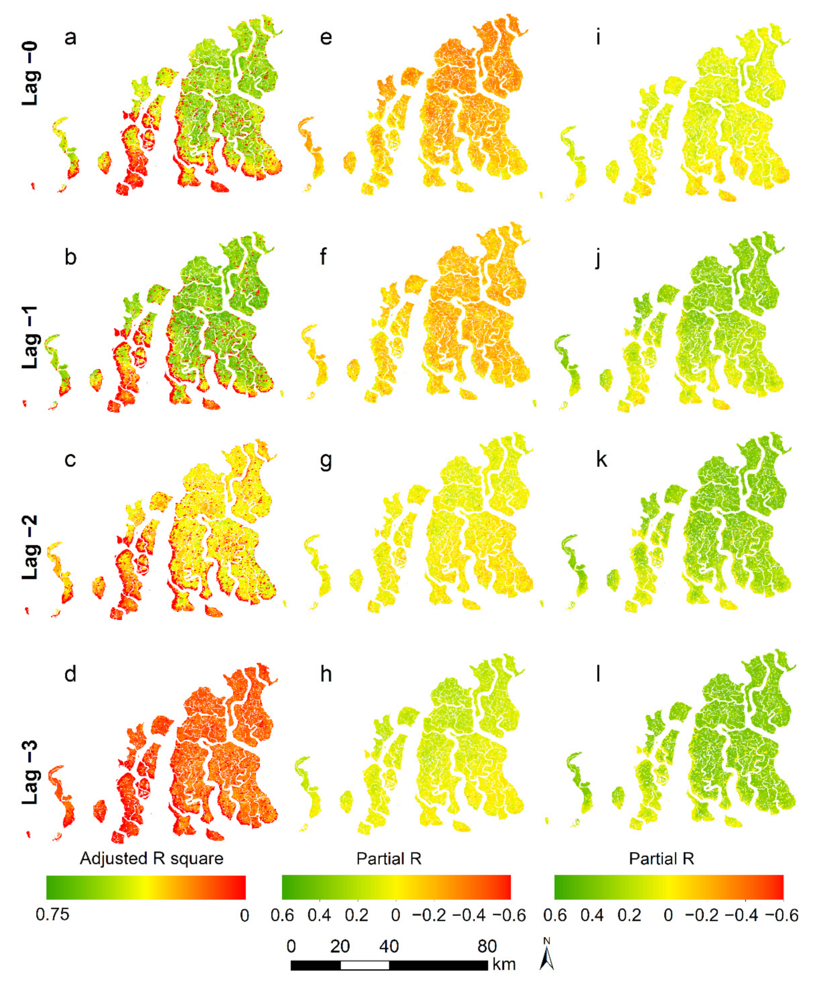
2.6. Relation of Vegetation Health Indicators to Climate Variability

Climate data were resampled to the 250 m spatial resolution of MODIS data for further analysis. The time series of the filtered VI dataset, as well as the resampled climatic variables, were constructed by averaging the 16-day and daily datasets at monthly and subsequently seasonal intervals (December–January–February: winter; March–April–May: summer; June–July–August: monsoon; September–October–November: post-monsoon), for further trend analysis and linear modeling. We performed a pixel-based time-series trend analysis—the non-parametric monotonic trend (Mann–Kendall statistics) [63]—to detect increases and decreases in the vegetation health indicators. The time-series relationships between VI and climatic variables (maximum and minimum temperatures and rainfall) were analyzed through multiple regression at different time lags. A total of 4 different time lags were used, namely lag-0, lag-1, lag-2, and lag-3, which correspond to the same month, previous month, 2 months prior, and 3 months prior, respectively.

2.7. Relation of Vegetation Health Indicators to Cyclone Impact

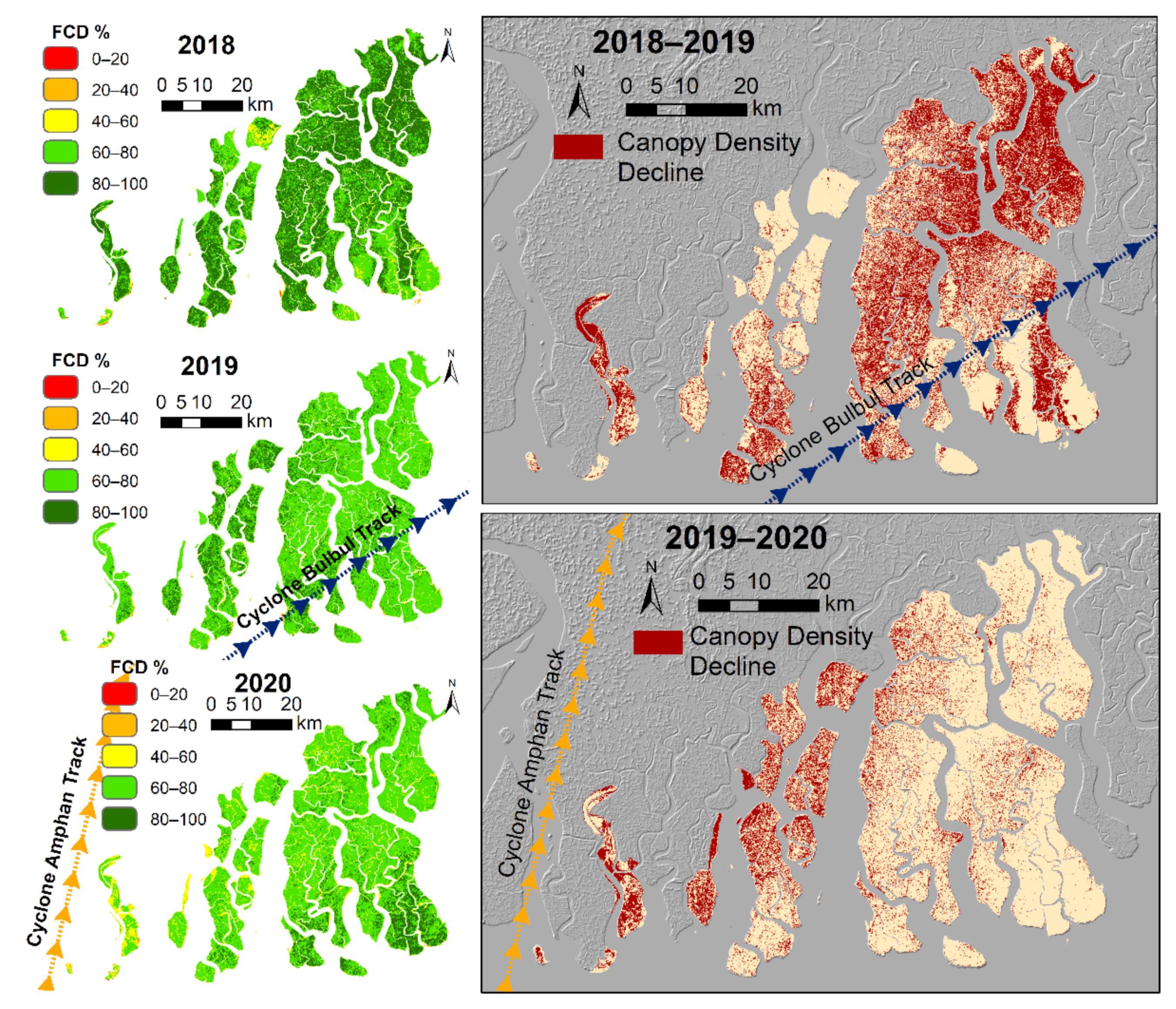
2.7.1. Canopy Density
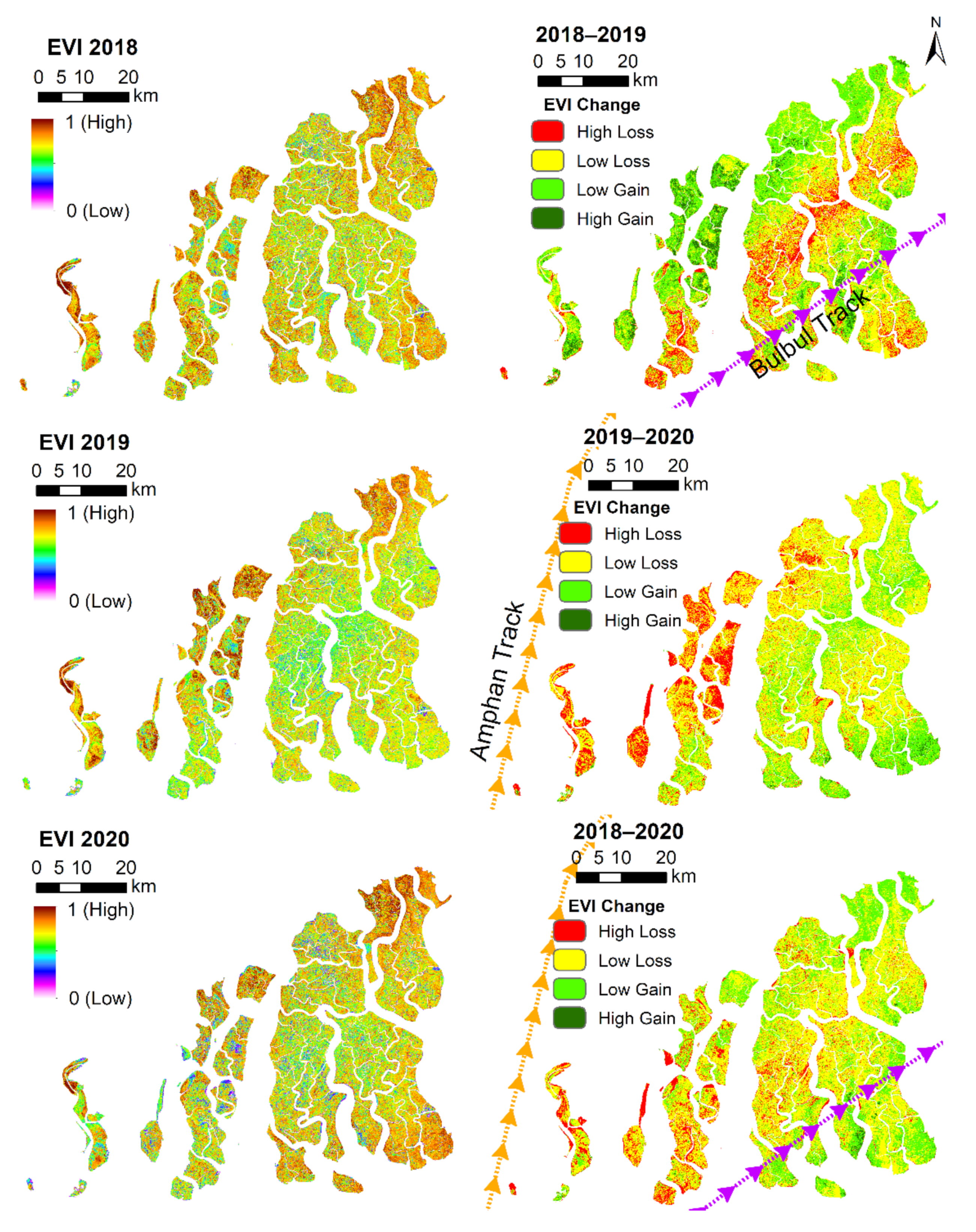
Landsat OLI images from before and after Cyclone Bulbul (2019) and the particularly intense Cyclone Amphan (2020) were used for measuring the forest canopy density (FCD) change. The FCD serves as a vital parameter for the characterization of mangrove conditions. This model includes bio-spectral modeling and analysis using data derived from four indices, viz. advanced vegetation index (AVI), bare soil index (BI), shadow index (SI) or scaled shadow index (SSI), and thermal index (TI) [44,64]. The percentage canopy density in each pixel was calculated by this method, and this forest canopy measure is valuable for cyclone damage assessment and evaluation of changing forest health over time.

2.7.2. EVI

EVI was calculated on atmospherically corrected Landsat OLI images pre- and post-Cyclones Bulbul and Amphan, using Equation (1) [31], as follows:
EVI = 2.5 × ((Band 5 − Band 4)/(Band 5 + 6 × Band 4 − 7.5 × Band 2 + 1))
where −1 < EVI < 1. The pre-cyclone and post-cyclone raster values were differenced, and the difference image was classified based on positive (health gain) and negative (health decline) values.

3. Results and Analysis

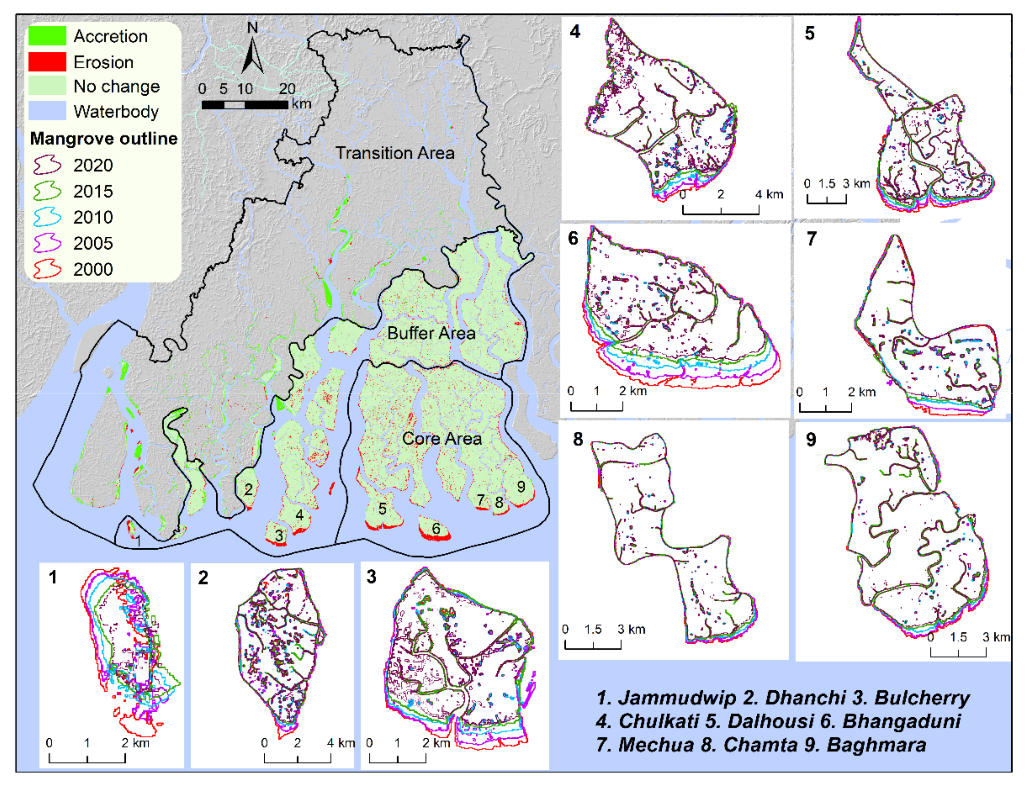
3.1. Change in Mangrove Forest Area

Analysis of the multi-temporal Landsat data from 2000 to 2020 showed significant erosion in the core and buffer areas (Figure 2) of the mangrove forest, accompanied by an increase in the transition area within human habitation. Around 110 km2 of mangroves were lost and 81 km2 gained in the SBR, corresponding to average losses and gains of 5.5 km2/year and 4.1 km2/year, respectively. The core area of the mangrove forest lost 58 km2 (2.9 km2/year), the buffer area lost 52 km2 (2.6 km2/year), while 81 km2 (4.1 km2/year) were gained in the transition area outside the contiguous mangrove area (Table 1). The rate of mangrove change was not uniform over time; the maximum loss rate was observed from 2000 to 2005 with losses of 4.5 km2/year in the core area and 3.4 km2/year in the buffer area, while maximum accretion was observed from 2015 to 2020 (7.7 km2/year).
Shoreline changes on nine ocean-facing islands, where the erosion is concentrated, were analyzed in detail (Figure 2 and Table 2). Land loss between 2000 and 2020 ranged from 1.3 km2 in Jammudwip to 11.6 km2 on Dalhousi Island. There was a net total loss of 49 km2 from these sea-facing islands, all of which (except Jammudwip Island) provide tiger habitats.

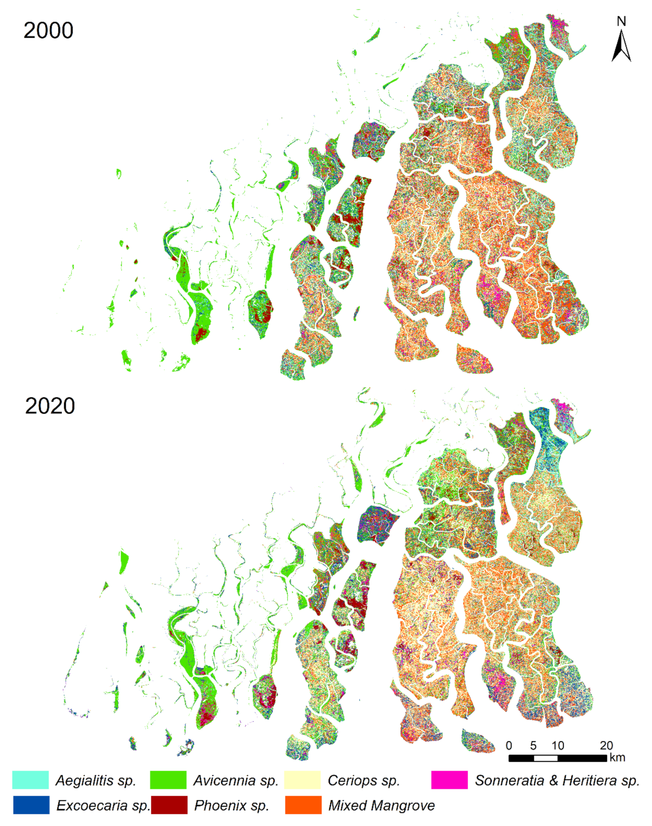
3.2. Changes in Mangrove Community Composition

Mangrove community composition maps were generated at the genus level for the years 2000 and 2020 (Figure 3). The results (summarized in Table 3) reveal an increase in salt-tolerant mangrove genera and a slight decline in the low salinity-loving genera. The largest increase in extent was for Ceriops sp.-dominated assemblage (4.2%), followed by Avicennia sp. (1.8%), Excoecaria sp. (1.4%), and Phoenix sp.-dominated assemblage (0.4%). Declines in area were observed from mixed mangrove class (5.7%), followed by Sonneratia-Heritiera sp. assemblages (1.5%) and Aegialitis sp. dominated assemblage (0.6%). The increase in Avicennia sp. assemblages can be attributed to the plantation along the riverbank and colonization of newly emerged Char/mudflat in transition areas.

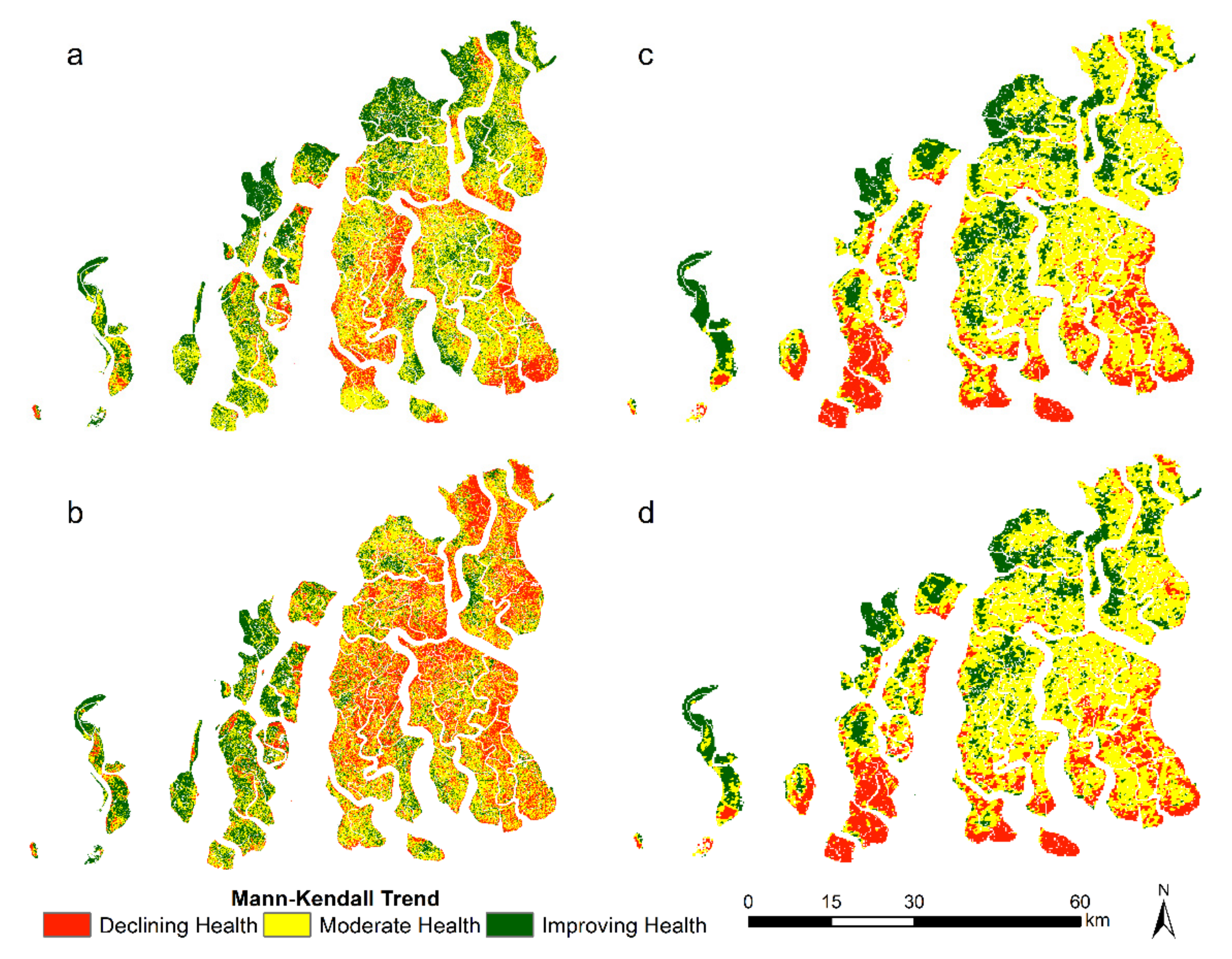
3.3. Change in Mangrove Health Indicators

Monotonic trends were computed for both Landsat and MODIS image sequences from 2000–2020. Due to the lack of cloud-free Landsat images, we conducted the MK test in the winter season only, whereas the monthly trend of NDVI–EVI was computed from MODIS data. The monotonic trend for the winter season shows a continuous decrease in EVI and NDVI values for both Landsat and MODIS, which indicates a progressive decline in the health of the mangrove forest. The Mann–Kendall trend test indicates that in the winter season Landsat analysis, 23% of NDVI pixels and 40% of EVI pixels showed a negative trend. However, 73% of NDVI pixels and 81% of EVI pixels showed a negative trend in the monthly MODIS analysis. Looking at the spatial distribution of the MK trend, a large decline on the sea-facing islands and in the central, eastern, and northeastern parts of the mangrove forest is apparent from the negative trend in NDVI and EVI. However, positive NDVI and EVI MK trends in western and some northern island margins were noted (Figure 4).
The existence of any relationships between EVI as a proxy for mangrove health and rainfall and the maximum air temperature was investigated through a correlation performed at four time monthly lags (lag-0 = same month, lag-1 = previous month, etc.). The adjusted R2 was high for lag-0 and lag-1 (adjusted R2 = 0.5–0.7) but declined for lag-2 and lag-3.

3.4. Drivers of Change

A range of drivers potentially influences the observed changes in the mangrove area, community structure, composition, and health. As summarised in Table 4, these include progressive legacy drivers due to a continued response to changes that have already happened, progressive contemporary drivers due to active ongoing changes, and shocks due to extreme events.

3.4.1. Sediment Supply

Due to the easterly tilt of the basin by block faulting, in the early 16th century, the main flow of the river Ganges shifted eastward [74], leaving the southerly flowing distributaries, such as Bhagirathi–Hugli on the west and Ichamati on the east of the Indian Sundarbans, dry outside the monsoon months. The most recent and largest intervention in the sediment and the freshwater dispersal system has been the building of the Farakka dam in 1975, which impounded 87 million m3 of water and sediments [75]. The dam not only initiated sedimentation upstream of the barrage but also considerably reduced (by approximately 31% [76]) the sediment supply downstream of the Hugli and its distributaries [77]. The lack of fresh water in the forest and sediment supply to the delta front contributes to other influences on mangrove health at a regional scale, being the major driver of increasing salinity (see below), and erosion of seaward facing shorelines against a background of sea-level rise.

3.4.2. Salinization

The increase in salinity in the estuaries of the Sundarbans is regarded as an environmental stressor, affecting the health of the mangroves and their services. Disconnection in the 20th century of major freshwater distributaries, such as Adi Ganga, Matla, Jamuna, Bidydhari, or Ichamati, from their freshwater sources, led to increased salinity ingress in the estuarine channels. Eleven such major disconnections, both natural and anthropogenic, have been identified from the field and remote sensing studies [78]. While the rising salinity level in the River Hugli, a major freshwater supplier to the megacity of Kolkata, was arrested and reversed after the freshwater supply was restored through the feeder canal at the Farakka dam, the salinity level in the Saptamukhi–Matla–Thakuran estuary or the Ichamati–Raimangal estuary, encompassing the Sundarban mangrove forest, has continued to increase over the last few decades.
Synthesizing observations of salinity in the Hugli–Saptamukhi–Matla–Thakuran–Raimangal estuaries, Mitra et al. [79] observed an acute scarcity of freshwater from the limited data around the core area of the Sundarbans. Salinity now remains as high as 13 ppt even during the monsoon, rising to 21 ppt in the post-monsoon period and up to 28 ppt in the pre-monsoon lean periods [80]. The literature indicates that the mangrove trees are at present subject to salt stress, which is manifested by stunted growth, reduced physiological functioning, and degradation of forest cover in several places. The freshwater-loving mangrove species (such as Heritiera fomes, Nypa fruiticans, Xylocarpus sp., and Sonneratia caseolaris) are widely diminishing and being replaced by more salt-tolerant species (Ceriops sp., Avicennia sp., and Excoecaria agallocha). This transition is also resulting in a net loss of species biodiversity.
Mitra et al. [79] reviewed published water salinity data within seven zones in the Sundarban Biosphere reserve area (Figure 5A). Figure 5B shows that, in the sea-facing SWS and SES zones that host the core and buffer areas of the Biosphere reserve, MODIS-derived mangrove health indicators show a significant deterioration over the period 2000–2020. In these zones, the salinity was observed to be 27–28 ppt during the pre-monsoon period and 17–21 ppt during the post-monsoon period, with an increasing trend in the last 30 years. In the NES zone along the Bangladesh border, despite high mean salinity, the health deterioration of the mangroves is moderate, due to the intermittent freshwater flow from the river Ichhamati. Similarly, healthy mangroves occur in the western part of Sundarbans due to some freshwater influx from the Hugli estuary through the Saptamukhi river. Declining mangrove cover and changing genus composition (which are considered to indicate degradation of mangrove health), due to increasing salinity, were observed by Chowdhury et al. [69] in the Indian Sundarbans. Rahman [45] studied the decline of some of the mangrove species (i.e., Heritiera fomes, Nypa fruticans, Phoenix paludosa), due to increasing salinity in the Bangladesh Sundarbans.

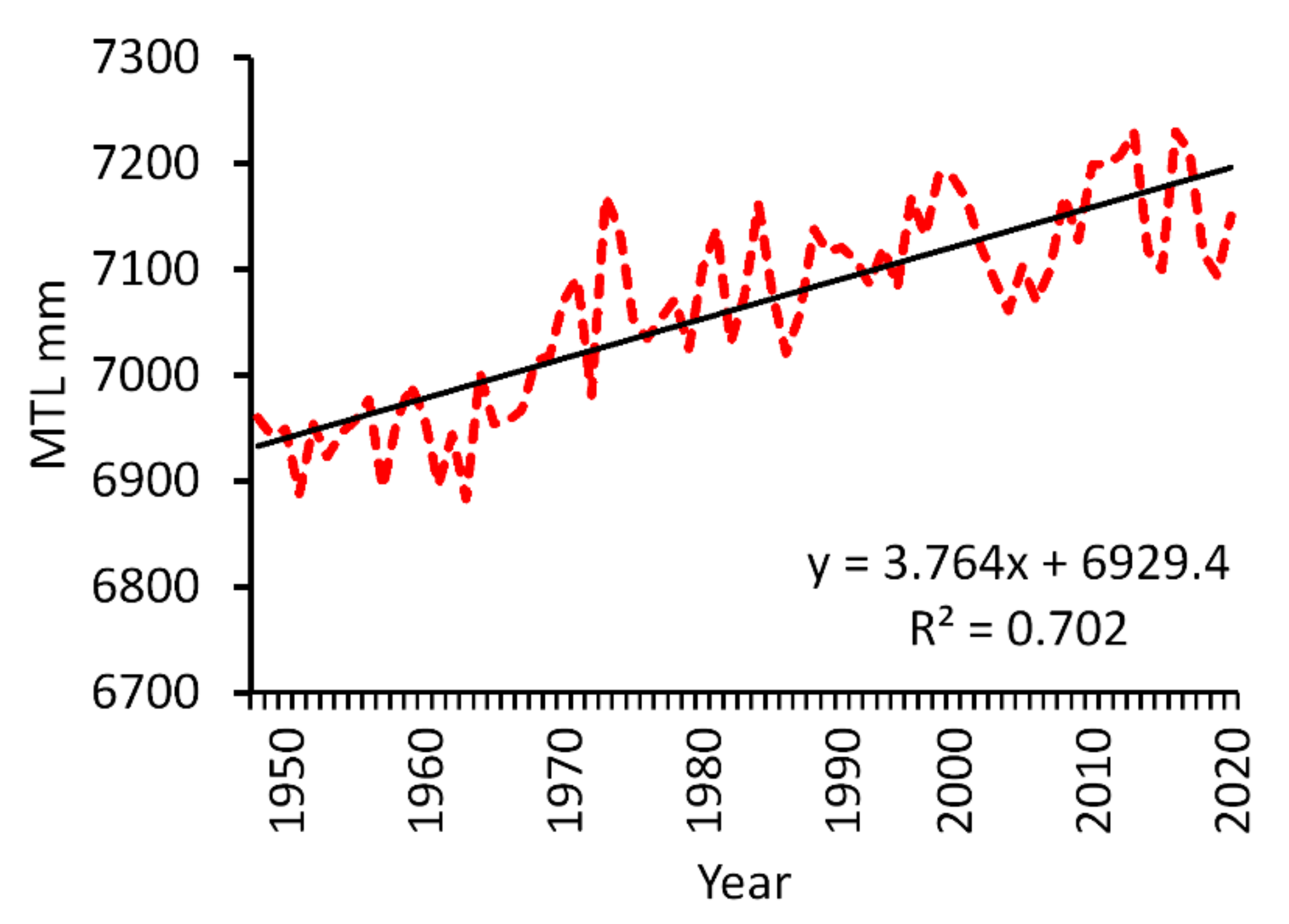
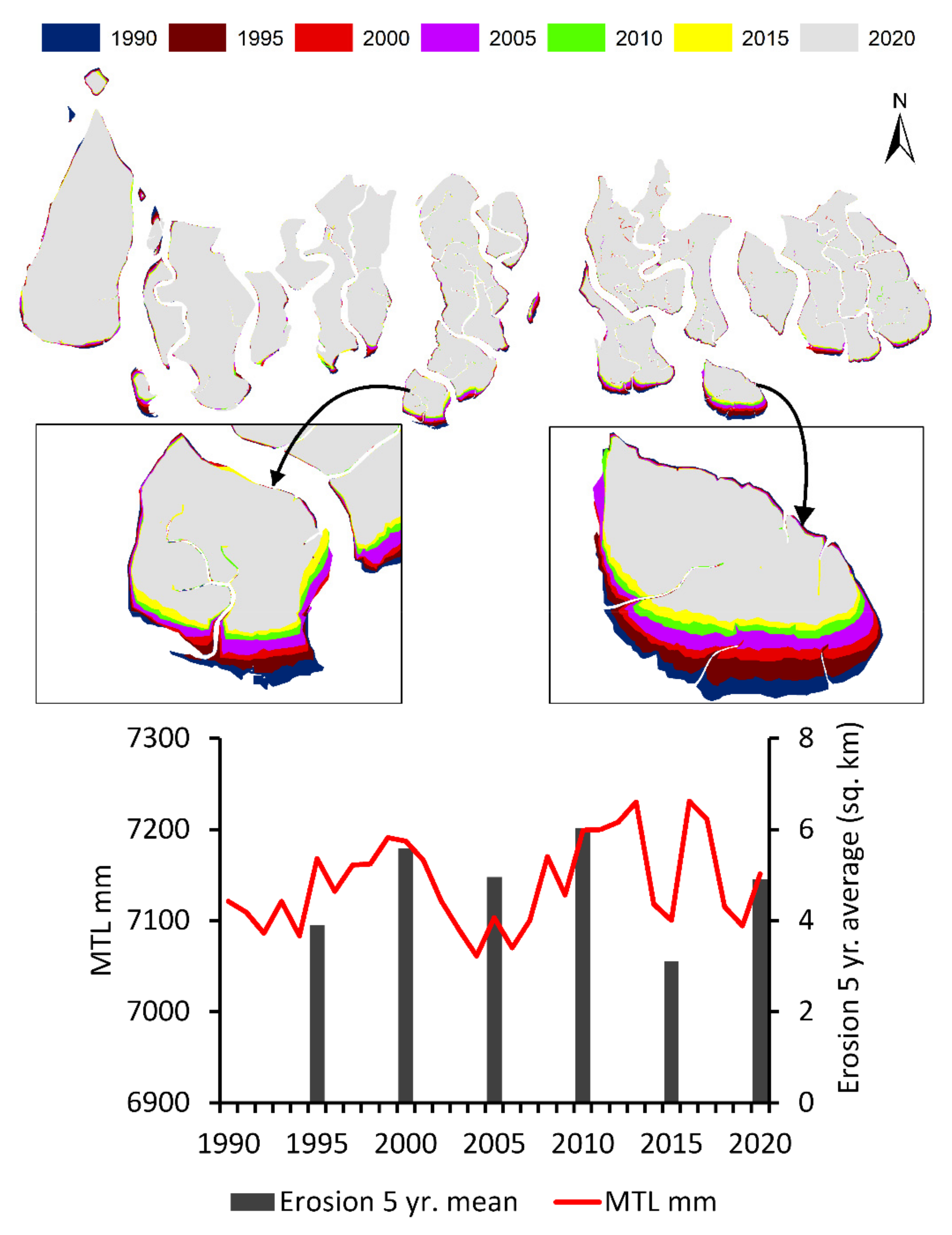
3.4.3. Relative Sea-Level Rise

Given its location on a major delta, the Sundarbans is exposed to both absolute sea-level rise and subsidence [80]. Tide gauge records in the northern Bay of Bengal show strong interannual variability in mean sea level associated with El Niño Southern Oscillation (ENSO) and Indian Ocean Dipole (IOD) influences, as well as variation river flow [81]. The longest and most complete of the Indian records is for Diamond Harbor on the Hugli estuary, which shows a linear trend of 3.75 mm/year for the period 1948–2020 (Figure 6). The tidal range here is approximately 5 m and the record also contains some variation at the scale of the 18.6-year nodal cycle. The sea-level rise trend at Diamond Harbor is broadly consistent with a trend in absolute sea-level of 3.11 ± 0.44 mm/year in the northern Bay of Bengal for the period 1993–2010, determined from analysis of satellite altimetry data by Ghosh et al. [82]; however, this can be assumed to include a contribution from subsidence as well. Subsidence is known to be significant but spatially variable across the delta [81,82]. Reliable data are sparse, but most estimates for the western part of the delta (including the Sundarbans) are around 2.5 to 4 mm/year [83,84,85], and this needs to be added to estimated (or projected future) change in absolute mean sea level in the region to evaluate the likely impact on the delta and its ecosystems. These impacts can be expected to include an increased tendency towards shoreline erosion (especially on ocean-facing islands in the delta), increased inundation, and more extensive influence of marine salinity.
Sea-level rise is widely associated with an increased tendency towards erosion along unprotected shorelines [85]. This hypothesis was investigated through an empirical analysis of shoreline changes, along with the ocean-facing islands of the Sundarbans, in comparison with trends in sea level for a slightly extended period from 1990 to 2020. Analyses of this kind are usually complicated by the strong interannual variability in sea level and also in erosion, which is driven by individual storm events that occur in conjunction with sea-level change. The results (Figure 7) show that significant erosion and land loss are occurring and that the rate of land loss exhibits a close correspondence with short-term fluctuations in mean sea level. The high rates of erosion can be attributed not only to the effect of storms but also to lower sediment availability within the Indian Sundarbans, compared with those in the neighboring Bangladesh (Table 4) [85].

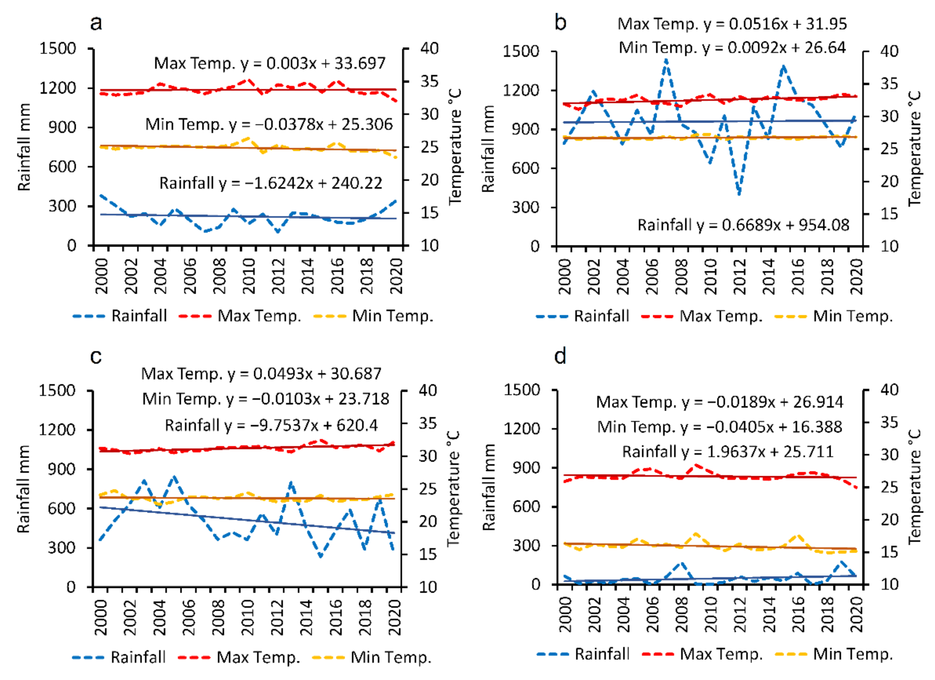
3.4.4. Changes in Air Temperature

Temperature is well established as a factor controlling the distribution of mangroves, with low temperatures being important in defining their latitudinal limits [86]; although, this is not an issue in the Sundarbans. Extreme high temperatures can also affect the survival and growth of mangrove seedlings [87]. Trends in seasonal air temperature over Sundarbans are shown in Figure 8. This analysis reveals upward trends in maximum air temperature in Summer (March, April, and May), monsoon (June, July, and August), and post-monsoon (September, October, and November). It is notable that high sea surface temperatures (SST) were recorded during the consecutive El Nino years of 2005, 2009–10, and 2015, which is reflected in the air temperature series presented here. Although the physiological mechanisms that cause reduced growth and mortality are still not fully understood [86], likely impacts of higher maximum temperatures include desiccation and adverse effects on plant metabolism during germination and propagation time (from July to September). Experimental work (e.g., [88]) has shown that even small changes in temperature extremes can have a significant effect on the health of mangrove seedlings, and in the Sundarbans, that could impact not only the health and functioning of the mangrove community but also the overall health of the wider ecosystem.
A partial correlation between mangrove EVI and maximum temperature shows a stronger negative response at lag-0 (30 days), implying that EVI is decreasing, with increasing maximum air temperature. It should be emphasized here that the literature on temperature effects on mangroves [87,88] suggests that these mainly involve the viability and health of seedlings; whereas, EVI is more representative of the health of the established mangrove canopy. Therefore, the present findings presumably reflect short-term stress experienced by the established mangrove forest, rather than providing evidence that climate change is limiting mangroves at the replacement or colonization stage.

3.4.5. Changes in Rainfall

A proportion of 70–80% of annual rainfall in the Sundarbans occurs during the summer monsoon (southwest monsoon), resulting in higher river discharge in the Hugli (range 2952 to 11,897 m3 s−1) and often in the Ichamati, which is found to decline steadily during non-monsoonal months (varying from 900 to 1500 m3 s−1) [89]. Rainfall variability is a major driver of temporal and spatial variation in salinity in the delta, and any changes in the river flow regime could have significant implications for the health of the mangrove forest and forest-dependent livelihoods. The present analysis indicates that, over the last two decades, there has been a decline in summer and post-monsoon rainfall, while monsoon rainfall has remained nearly constant, followed by a slight increase in winter rainfall (Figure 8). Reduced rainfall, both in the summer and the post-monsoon season, is likely to have a negative influence on the health of the mangroves by reinforcing an increase in salinity, as already discussed.
The partial correlation between EVI and rainfall was strongly negative at lag-0 and lag-1, with a weaker positive correlation observed at lag-2 and lag-3 (Figure 9). This implies that rainfall has no immediate effect on plant health but may affect the health of the mangrove with a longer response interval (2/3 months). However, a strong correlation (R2 = 0.7) observed between the combined effect of rising temperature and rainfall variability (especially reduced rain in the pre-monsoon and post-monsoon) with the declining trend of EVI or mangrove health indicates that, along with other drivers, such as increasing salinity and sea level, a changing climatic pattern might have a significant contribution to the degradation of mangrove health.

3.4.6. Short-Term Degradation Due to Cyclones

In addition to progressive trends in sea level and climate variables, frequent cyclones and associated coastal flooding by storm surges are the major natural hazards in the delta. The Bay of Bengal experiences 7% of the major cyclones of the world [90]. Over the last 120 years, there has been a 26% increase in the number of very severe cyclonic storms over the northern Bay of Bengal [91] and increases in both frequency and intensity have been observed for the last two decades in particular [92,93,94].
In the early years of the 21st century, a sharp rise of SST has been associated with seven such cyclonic storms in the northern Bay of Bengal, including Mala (in 2006), Sadr (in 2007), Bijli (in 2009), and Aila (in 2009)—four storms in less than four years, which impacted large areas in the Sundarbans. In the last decade (2011–20), the delta has suffered the impacts of Roanu (2016), Titli (2018), Fani (2019), Bulbul (2019), and Amphan (2020). The Sundarbans narrowly escaped the devastating Phalin (2013) and Hudhud (2014) cyclones. The present study assessed the damages to the mangrove forests in Sundarbans during the severe cyclonic storm Bulbul and very severe cyclone storm Amphan, which occurred less than six months apart. Avoiding the seasonal variability of mangrove plant phenology, we analyzed the Landsat 8 and Sentinel-2 satellite data to assess the changes in the pre-cyclone and post-cyclone mangrove forest canopy density (FCD). Advanced vegetation index, bareness index, shadow index, and thermal index were computed and compared. It was observed (see Figure 10) that FCD decreased considerably in the 80–100% FCD classes after Cyclone Bulbul on 9 November 2019 and Amphan on 20 May 2020. Detailed analysis shows that 780 km2 changed from very high (80–100%) to high canopy density (60–80%) and a small fraction converted from high to moderate canopy density (40–60%) between 2018 and 2019 (pre-Bulbul and post-Bulbul). In comparison, 261 km2 changed from very high to high canopy density and 142 km2 from high to moderate canopy density between 2019 and 2020 (pre-Amphan and post-Amphan).
As shown in Figure 11, enhanced vegetation index (EVI), derived from Landsat 8 data, also indicated a considerable reduction in mangrove health along the tracks of the consecutive cyclones. Proportions of 14.6% (303.6 km2) and 45.8% (950.7 km2) of the area suffered high and low loss, respectively, after Cyclone Bulbul. The changes were broadly similar with 14% (287 km2) high loss and 51% (1064 km2) low loss after Cyclone Amphan. The combined effect over the whole period spanning both cyclones was 13.3% (277 km2) high loss and 57.4% (1190 km2) low loss. Cyclones cause severe damage to the mangrove canopy with limited recovery between severe storms occurring in close succession. These findings imply that the observed increased frequency of high-intensity cyclones in the Bay of Bengal is having adverse consequences on mangrove health [95,96].

4. Discussion

The present study has shown that about 110 km2 mangrove forest area was lost during the period 2000–2020. Critically analyzing the spatial distribution of land loss, we observed that the majority of the loss of mangroves took place in the core region of the National Park and tiger reserve. However, in the fringe area outside the contiguous forest, a gain of 81 km2 of mangroves occurred. This opens up a new question of whether the forest area loss and subsequent habitat and blue carbon services can be compensated by mangrove plantation and regeneration. To estimate the loss of blue carbon over the last two decades, we used the estimate of Ray et al. [97], that the average aboveground and belowground biomass in the Indian Sundarbans is 39.93 ± 14.05 t C ha−1 and 9.61 ± 3.37 t C ha−1, respectively. Assuming this estimate holds for the lost mangrove cover, an estimated 0.29 × 10⁶ t C and 0.072 × 10⁶ t C have been lost from the aboveground and the belowground stores, respectively. A total of 0.36 × 10⁶ t C is estimated to have been lost due to the loss of just the mangrove floral stand. A portion of the mangrove soil will have been lost due to erosion, with a further loss of the carbon trapped in the sediments. The spatial variability of soil sediment carbon is high and is harder to estimate than the species-specific carbon stock. However, these figures provide at least a first order estimate of the carbon storage that needs to be replaced through plantation and regeneration schemes.
The analysis presented here includes the first attempt to relate observations of mangrove health degradation with rising maximum air temperature and declining post-monsoon rainfall in the Indian Sundarbans region. In addition, the impact of repeated cyclones (2 out of 4 in 24 months that took place at intervals of 6 months) has been analyzed to demonstrate the consequences of more frequent high-intensity cyclones. The mangroves, as observed after cyclone Sidr in Bangladesh, took 6–7 years to recover from the damage. Temperature rise, a decline of post-monsoon rainfall, and a higher frequency of cyclonic incidence in this part of the delta have adversely impacted the health of the mangroves in Sundarbans.
While the impact of high soil and estuarine salinity seems to have promoted stunted growth, lower above-ground biomass and health degradation, and near absence of freshwater-loving species like Heritiera, Nypa, or Sonneratia from the Indian Sundarbans, in the absence of time series data of soil salinity, any specific correlation of rising soil salinity with the health degradation of mangroves is not possible. However, lower health mangroves were observed in saline sea-facing situations, while healthier mangroves are observed in the buffer region where some freshwater input occurs from the river Hugli on the west or river Ichamati on the eastern fringe. This requires further investigation.
The present research highlights two important aspects of mangrove degradation within the Sundarbans region of the Ganges–Brahmaputra delta. The first is the high rate of relative sea-level rise in the absence of adequate sediment supply to the delta causing significant loss of mangrove area over the last two decades. The second is the decline in health of the existing mangroves due to reduced freshwater supply, the rise of salinity (which is also enhanced buy sea-level rise), and the combined effect of rainfall instability and temperature rise. Both these sets of drivers have led to significant loss of tiger habitat and blue carbon stock. This degradation and loss are expected to continue and likely accelerate with rising sea levels. This observation warrants the immediate attention of planners and policymakers, who need to change to ecosystem-based management and restoration of this global heritage site. One positive finding that emerges from this study, however, is the growth of fringe mangroves around the inhabited islands in the inner estuaries, thanks to plantation and restoration efforts by government agencies, NGOs, and local communities. Extensive regeneration of mangroves with an appropriate salinity tolerance is an immediate option where space is available, even on mudflats around islands within mangrove forest areas of the outer estuary. This can be further supported by the installation of submerged oyster reefs or breakwater to arrest erosion and offshore silt loss, which has apparently been successful in Kutubdia island in Bangladesh on the eastern delta. However, as a long-term ecosystem regeneration strategy to improve the health of the mangroves, action to combat the rise of salinity and nutrient deficiency is a prerequisite, particularly when facing climate change. Earlier research [98] indicated that provisioning of around 500 m3 s−1 of freshwater through the restoration of moribund river channels and intra-basinal water transfer is a feasible option. However, this may require a transboundary management approach in collaboration with Bangladesh.

5. Conclusions

This analysis shows that the Sundarbans mangroves are experiencing a slow decline in terms of both area and key health indicators. Shoreline erosion on the ocean-facing islands has been the dominant mechanism of areal loss over the period 2000–2020. Changes in the composition of the mangrove forest community are also evident, with a shift towards more salt-tolerant species occurring in response to decreased freshwater influx from precipitation and river flow, in conjunction with increasingly estuarine conditions as a result of sea-level rise. The persistent decline of mangrove health indicators in the major part of the forest associated with salinity stress, and possibly also trends in maximum air temperature and rainfall variability, are another concern. Major cyclones are also shown to cause extensive damage along their tracks and recovery can be limited when severe storms occur in close succession. Although the net losses remain small in percentage terms, there is potential for a more significant and sustained decline, given the expectation of an acceleration in the rate of sea-level rise and a reduction in frequency (and therefore increased ‘clustering’) of extreme cyclone events. Further work, including continued systematic monitoring, is required to fully assess the implications for the future sustainability of the vital Sundarbans ecosystem.

Author Contributions

Conceptualization, S.S. and S.H.; methodology, S.S. and P.P.M.; software, S.S. and P.P.M.; validation, S.S., S.H., P.P.M., A.C. and S.G.; formal analysis, S.S., S.H., P.P.M., A.C. and S.G.; investigation, S.S., S.H., P.P.M., A.C. and S.G.; data curation, S.S., S.H., P.P.M., A.C. and S.G.; writing—original draft preparation, S.S., S.H., J.R.F. and R.J.N.; writing—review and editing, J.R.F. and R.J.N.; visualization, S.S.; supervision, S.H.; project administration, S.H.; funding acquisition, S.H. and R.J.N. All authors have read and agreed to the published version of the manuscript.

Funding

This research was funded under the “Towards a Sustainable Earth: Environment-human systems and the UN Global Goals” (TaSE) program in the project “Opportunities and trade-offs between the SDGs for food, welfare and the environment in deltas”. Funding was provided by NERC Grant NE/S012478/1, Formas Grant 2019-00045, and the UKIERI-DBT (Grant No. BT/IN/TaSE/70/SH/2018-19) under UK-India Education Research Initiative.

Institutional Review Board Statement

Not applicable.

Informed Consent Statement

Not applicable.

Data Availability Statement

The data presented in this study are available on request from the corresponding author. No new data have been created in this study, rather, the existing data of several types from multifarious sources have been modeled and analyzed in the present study. Requests to share the data analyzed in this study can be sent to the corresponding author in case of specific interests.

Acknowledgments

The authors acknowledge the State Forest Department of West Bengal, India, and the local inhabitants of the Sundarbans Biosphere Reserve for extending their help time and again to accomplish research of this nature. The authors are also grateful to the respective agencies that provided the remotely sensed data to carry out this study.

Conflicts of Interest

The authors declare no conflict of interest.

References

  1. Giri, C.; Ochieng, E.; Tiszen, L.L.; Zhu, Z.; Singh, A.; Loveland, T.; Masek, J.; Duke, N. Status and distribution of mangrove forests of the world using earth observation satellite data. Glob. Ecol. Biogeogr. 2010, 20, 154–159. [Google Scholar] [CrossRef]
  2. Alongi, D.M. The Energetics of Mangrove Forests; Springer: Dordrecht, The Netherlands, 2009. [Google Scholar]
  3. Field, C.B.; Osborn, J.G.; Hoffman, L.L.; Polsenberg, J.F.; Ackerly, D.D.; Berry, J.A.; Björkman, O.; Held, A.; Matson, P.A.; Mooney, H.A. Mangrove biodiversity and ecosystem function. Glob. Ecol. Biogeogr. Lett. 1998, 7, 3–14. [Google Scholar] [CrossRef]
  4. Dodd, R.S.; Ong, J.E. Future of mangrove ecosystems to 2025. In Aquatic Ecosystems: Trends and Global Prospects; Polunin, N.V.C., Ed.; Cambridge University Press: Cambridge, UK, 2008; pp. 172–187. [Google Scholar]
  5. Nagelkerken, I.; Blaber, S.J.M.; Bouillon, S.; Green, P.; Haywood, M.; Kirton, L.G.; Meynecke, J.-O.; Pawlik, J.; Penrose, H.M.; Sasekumar, A.; et al. The habitat function of mangroves for terrestrial and marine fauna: A review. Aquat. Bot. 2008, 89, 155–185. [Google Scholar] [CrossRef] [Green Version]
  6. Wolanski, E. Transport of sediment in mangrove swamps. In Asia-Pacific Symposium on Mangrove Ecosystems. Developments in Hydrobiology; Wong, Y.S., Tam, N.F.Y., Eds.; Springer: Dordrecht, The Netherlands, 1995; Volume 106. [Google Scholar] [CrossRef]
  7. Dittmar, T.; Hertkorn, N.; Kattner, G.; Lara, R.J. Mangroves, a major source of dissolved organic carbon to the oceans. Glob. Biogeochem. Cycles 2006, 20, GB1012. [Google Scholar] [CrossRef]
  8. Zhang, K.; Liu, H.; Li, Y.; Xu, H.; Shen, J.; Rhome, J.; Smith, T.J. The role of mangroves in attenuating storm surges. Estuar. Coast. Shelf Sci. 2012, 102–103, 11–23. [Google Scholar] [CrossRef]
  9. Arkema, K.K.; Guannel, G.; Verutes, G.; Wood, S.A.; Guerry, A.; Ruckelshaus, M.; Kareiva, P.; Lacayo, M.; Silver, J.M. Coastal habitats shield people and property from sea-level rise and storms. Nat. Clim. Chang. 2013, 3, 913–918. [Google Scholar] [CrossRef]
  10. Menéndez, P.; Losada, I.J.; Torres-Ortega, S.; Narayan, S.; Beck, M.W. The Global Flood Protection Benefits of Mangroves. Sci. Rep. 2020, 10, 4404. [Google Scholar] [CrossRef]
  11. Donato, D.C.; Kauffman, J.B.; Murdiyarso, D.; Kurnianto, S.; Stidham, M.; Kanninen, M. Mangroves among the most carbon-rich forests in the tropics. Nat. Geosci. 2011, 4, 293–297. [Google Scholar] [CrossRef]
  12. Alongi, D.M. Carbon cycling and storage in mangrove forests. Annu. Rev. Mar. Sci. 2014, 6, 195–219. [Google Scholar] [CrossRef]
  13. Duarte, C.M.; Losada, I.J.; Hendriks, I.E.; Mazarrasa, I.; Marbà, N. The role of coastal plant communities for climate change mitigation and adaptation. Nat. Clim. Chang. 2013, 3, 961–968. [Google Scholar] [CrossRef] [Green Version]
  14. Valiela, I.; Bowen, J.L.; York, J.K. Mangrove forests: One of the world’s threatened major tropical environments. Bioscience 2001, 51, 807–815. [Google Scholar] [CrossRef] [Green Version]
  15. Thomas, N.; Lucas, R.; Bunting, P.; Hardy, A.; Rosenqvist, A.; Simard, M. Distribution and drivers of global mangrove forest change, 1996–2010. PLoS ONE 2017, 12, e0179302. [Google Scholar] [CrossRef] [Green Version]
  16. Polidoro, B.A.; Carpenter, K.E.; Collins, L.; Duke, N.C.; Ellison, A.M.; Ellison, J.C.; Farnsworth, E.J.; Fernando, E.S.; Kathiresan, K.; Koedam, N.E.; et al. The loss of species: Mangrove extinction risk and geographic areas of global concern. PLoS ONE 2010, 5, e10095. [Google Scholar] [CrossRef]
  17. Hamilton, S.E.; Casey, D. Creation of a high spatio-temporal resolution global database of continuous mangrove forest cover for the 21st century (CGMFC-21). Glob. Ecol. Biogeogr. 2016, 25, 729–738. [Google Scholar] [CrossRef]
  18. Goldberg, L.; Lagomasino, D.; Thomas, N.; Fatoyinbo, T. Global declines in human-driven mangrove loss. Glob. Chang. Biol. 2020, 26, 5844–5855. [Google Scholar] [CrossRef]
  19. Doughty, C.L.; Langley, J.A.; Walker, W.S.; Feller, I.C.; Schaub, R.; Chapman, S.K. Mangrove range expansion rapidly increases coastal wetland carbon storage. Estuar. Coast. 2016, 39, 385–396. [Google Scholar] [CrossRef]
  20. Alongi, D.M. Mangrove forests: Resilience, protection from tsunamis, and responses to global climate change. Estuar. Coast. Shelf Sci. 2008, 76, 1–13. [Google Scholar] [CrossRef]
  21. Kuenzer, C.L.; Bluemel, A.; Gebhardt, S.; Quoc, T.V.; Dech, S. Remote sensing of mangrove ecosystems: A review. Remote Sens. 2011, 3, 878–928. [Google Scholar] [CrossRef] [Green Version]
  22. Simard, M.; Fatoyinbo, L.; Smetanka, C.; Rivera-Monroy, V.H.; Castañeda-Moya, E.; Thomas, N.; Van Der Stocken, T. Mangrove canopy height globally related to precipitation, temperature and cyclone frequency. Nat. Geosci. 2019, 12, 40–45. [Google Scholar] [CrossRef]
  23. Lee, S.-K. Mangrove height estimates from TanDEM-X data. Korea J. Rem. Sens. 2020, 36, 325–335. [Google Scholar] [CrossRef]
  24. Atwood, T.B.; Connolly, R.M.; Almahasheer, H.; Carnell, P.E.; Duarte, C.M.; Lewis, C.J.E.; Irigoien, X.; Kelleway, J.J.; Lavery, P.S.; Macreadie, P.I.; et al. Global patterns in mangrove soil carbon stocks and losses. Nat. Clim. Chang. 2017, 7, 523–528. [Google Scholar] [CrossRef]
  25. Tang, W.; Zheng, M.; Zhao, X.; Shi, J.; Yang, J.; Trettin, C.C. Big geospatial data analytics for global mangrove biomass and carbon estimation. Sustainability 2018, 10, 472. [Google Scholar] [CrossRef] [Green Version]
  26. Bryan-Brown, D.N.; Connolly, R.M.; Richards, D.R.; Adame, F.; Friess, D.A.; Brown, C.J. Global trends in mangrove forest fragmentation. Sci. Rep. 2020, 10, 7117. [Google Scholar] [CrossRef] [PubMed]
  27. Manna, S.; Raychaudhuri, B. Mapping distribution of Sundarban mangroves using Sentinel-2 data and new spectral metric for detecting their health condition. Geocarto Int. 2020, 35, 434–452. [Google Scholar] [CrossRef]
  28. Giri, C.; Pengra, B.; Zhu, Z.; Singh, A.; Tieszen, L.L. Monitoring mangrove forest dynamics of the Sundarbans in Bangladesh and India using multi-temporal satellite data from 1973 to 2000. Estuar. Coast. Shelf Sci. 2007, 73, 91–100. [Google Scholar] [CrossRef]
  29. Chellamani, P.; Prakash Singh, C.; Panigrahy, S. Assessment of the health status of Indian mangrove ecosystems using multi temporal remote sensing data. Tropic. Ecol. 2014, 55, 245–253. [Google Scholar]
  30. Pastor-Guzman, J.; Dash, J.; Atkinson, P.M. Remote sensing of mangrove forest phenology and its environmental drivers. Rem. Sens. Environ. 2018, 205, 71–84. [Google Scholar] [CrossRef] [Green Version]
  31. Huete, A.; Didan, K.; Miura, T.; Rodriguez, E.P.; Gao, X.; Ferreira, L.G. Overview of the radiometric and biophysical performance of the MODIS vegetation indices. Remote Sens. Environ. 2002, 83, 195–213. [Google Scholar] [CrossRef]
  32. Maryantika, N.; Lin, C. Exploring changes of land use and mangrove distribution in the economic area of Sidoarjo District, East Java using multi-temporal Landsat images. Info. Process. Agric. 2017, 4, 321–332. [Google Scholar] [CrossRef]
  33. Abd-El Monsef, H.; Smith, S.E. A new approach for estimating mangrove canopy cover using Landsat 8 imagery. Comp. Electron. Agric. 2017, 135, 183–194. [Google Scholar] [CrossRef]
  34. Ishtiaque, A.; Myint, S.W.; Wang, C. Examining the ecosystem health and sustainability of the world’s largest mangrove forest using multi-temporal MODIS products. Sci. Total Environ. 2016, 569–570, 1241–1254. [Google Scholar] [CrossRef]
  35. Rahman, M.M.; Rahman, M.M.; Islam, K.S. The causes of deterioration of Sundarban mangrove forest ecosystem of Bangladesh: Conservation and sustainable management issues. Aquac. Aquar. Conserv. Legis. 2010, 3, 77–90. [Google Scholar]
  36. Paul, A.K.; Ray, R.; Kamila, A.; Jana, S. Mangrove degradation in the Sundarbans. In Coastal Wetlands: Alteration and Remediation; Finkl, C., Makowski, C., Eds.; Springer: Cham, Switzerland, 2017; pp. 357–392. [Google Scholar] [CrossRef]
  37. Islam, M.J.; Alam, M.S.; Elahi, K.M. Remote sensing for change detection in the Sundarbans, Bangladesh. Geocarto Int. 1997, 12, 91–100. [Google Scholar] [CrossRef]
  38. Kundu, K.; Halder, P.; Mandal, J.K. Detection and prediction of sundarban reserve forest using the CA-Markov chain model and remote sensing data. Earth Sci. Inf. 2021, 14, 1503–1520. [Google Scholar] [CrossRef]
  39. Kundu, K.; Halder, P.; Mandal, J.K. Change Detection and Patch Analysis of Sundarban Forest During 1975–2018 Using Remote Sensing and GIS Data. SN Comput. Sci. 2021, 2, 1–14. [Google Scholar] [CrossRef]
  40. Chatterjee, N.; Mukhopadhyay, R.; Mitra, D. Decadal changes in shoreline patterns in Sundarbans, India. J. Coast Sci. 2015, 2, 54–64. [Google Scholar]
  41. Bera, R.; Maiti, R. Quantitative analysis of erosion and accretion (1975–2017) using DSAS—A study on Indian Sundarbans. Reg. Stud. Mar. Sci. 2019, 28, 100583. [Google Scholar] [CrossRef]
  42. Rahman, A.F.; Dragoni, D.; El-Masri, B. Response of the Sundarbans coastline to sea level rise and decreased sediment flow: A remote sensing assessment. Rem. Sens. Environ. 2011, 115, 3121–3128. [Google Scholar] [CrossRef]
  43. Sánchez-Arias, L.E.; Rodriguez, J.P.; Caballer, M.; Asmussen, M.V.; Medina, G. Diagnostic of health status in Mangrove ecosystems. Adv. Environ. Res. 2011, 3, 235–262. [Google Scholar]
  44. Sahana, M.; Sajjad, H.; Ahmed, R. Assessing spatio-temporal health of forest cover using forest canopy density model and forest fragmentation approach in Sundarban reserve forest, India. Model. Earth Syst. Environ. 2015, 1, 49. [Google Scholar] [CrossRef]
  45. Rahman, M.M. Impact of increased salinity on the plant community of the Sundarbans Mangrove of Bangladesh. Commun. Ecol. 2020, 21, 273–284. [Google Scholar] [CrossRef]
  46. Pitchaikani, J.S. Vertical current structure in a macro-tidal, well mixed Sundarban ecosystem, India. J. Coast Conserv. 2020, 24, 63. [Google Scholar] [CrossRef]
  47. Ali, S.A.; Khatun, R.; Ahmad, A.; Ahmad, S.N. Assessment of cyclone vulnerability, hazard evaluation and mitigation capacity for analyzing cyclone risk using GIS technique: A study on Sundarban biosphere reserve, India. Earth Syst. Environ. 2020, 4, 71–92. [Google Scholar] [CrossRef]
  48. Padhy, S.R.; Bhattacharyya, P.; Dash, P.K.; Reddy, C.S.; Chakraborty, A.; Pathak, H. Seasonal fluctuation in three mode of greenhouse gases emission in relation to soil labile carbon pools in degraded mangrove, Sundarban, India. Sci. Total Environ. 2020, 705, 135909. [Google Scholar] [CrossRef]
  49. Ghosh, A.; Schmidt, S.; Fickert, T.; Nüsser, M. The Indian Sundarban mangrove forests: History, utilization, conservation strategies and local perception. Diversity 2015, 7, 149–169. [Google Scholar] [CrossRef]
  50. Barik, J.; Chowdhury, S. True mangrove species of Sundarbans delta, West Bengal, eastern India. Check List 2014, 10, 329–334. [Google Scholar] [CrossRef]
  51. Barik, J.; Mukhopadhyay, A.; Ghosh, T.; Mukhopadhyay, S.K.; Chowdhury, S.M.; Hazra, S. Mangrove species distribution and water salinity: An indicator species approach to Sundarban. J. Coast. Conserv. 2018, 22, 361–368. [Google Scholar] [CrossRef]
  52. Banerjee, K.; Gatti, R.C.; Mitra, A. Climate change-induced salinity variation impacts on a stenoecious mangrove species in the Indian Sundarbans. Ambio 2017, 46, 492–499. [Google Scholar] [CrossRef] [Green Version]
  53. Wang, D.; Wan, B.; Qiu, P.; Su, Y.; Guo, Q.; Wang, R.; Sun, F.; Wu, X. Evaluating the performance of Sentinel-2, Landsat 8 and Pléiades-1 in mapping mangrove extent and species. Remote Sens. 2018, 10, 1468. [Google Scholar] [CrossRef] [Green Version]
  54. Giri, S.; Mukhopadhyay, A.; Hazra, S.; Mukherjee, S.; Roy, D.; Ghosh, S.; Ghosh, T.; Mitra, D. A study on abundance and distribution of mangrove species in Indian Sundarban using remote sensing technique. J. Coast. Conserv. 2014, 18, 359–367. [Google Scholar] [CrossRef]
  55. Ghosh, M.K.; Kumar, L.; Roy, C. Mapping long-term changes in mangrove species composition and distribution in the Sundarbans. Forests 2016, 7, 305. [Google Scholar] [CrossRef] [Green Version]
  56. Mitra, D.; Karmaker, S. Mangrove classification in Sundarban using high resolution multi-spectral remote sensing data and GIS. Asian J. Environ. Disaster Manag. 2010, 2, 197–207. [Google Scholar]
  57. Kumar, T.; Mandal, A.; Dutta, D.; Nagaraja, R.; Dadhwal, V.K. Discrimination and classification of mangrove forests using EO-1 Hyperion data: A case study of Indian Sundarbans. Geocarto Int. 2019, 34, 415–442. [Google Scholar] [CrossRef]
  58. Mukhopadhyay, A.; Wheeler, D.; Dasgupta, S.; Dey, A.; Sobhan, I. Aquatic salinization and mangrove species in a changing climate: Impact in the Indian Sundarbans. World Bank Policy Res. Work. Pap. 2018, 8532, 1–21. [Google Scholar]
  59. Hati, J.P.; Samanta, S.; Chaube, N.R.; Misra, A.; Giri, S.; Pramanick, N.; Gupta, K.; Majumdar, S.D.; Chanda, A.; Mukhopadhyay, A.; et al. Mangrove classification using airborne hyperspectral AVIRIS-NG and comparing with other spaceborne hyperspectral and multispectral data. Egypt. J. Remote Sens. Space Sci. 2021, 24, 273–281. [Google Scholar] [CrossRef]
  60. Didan, K. MOD13Q1 MODIS/Terra Vegetation Indices 16-Day L3 Global 250m SIN Grid V006. NASA EOSDIS Land Processes DAAC. 2015. Available online: https://lpdaac.usgs.gov/data/ (accessed on 6 June 2020).
  61. AppEEARS Team. Application for Extracting and Exploring Analysis Ready Samples (AppEEARS); Ver. 2.42.1; NASA EOSDIS Land Processes Distributed Active Archive Center (LP DAAC), USGS/Earth Resources Observation and Science (EROS) Center: Sioux Falls, SD, USA, 2020. Available online: https://lpdaacsvc.cr.usgs.gov/appeears (accessed on 6 June 2020).
  62. Kovács, F.; Gulácsi, A. Spectral index-based monitoring (2000–2017) in lowland forests to evaluate the effects of climate change. Geosciences 2019, 9, 411. [Google Scholar] [CrossRef] [Green Version]
  63. Neeti, N.; Eastman, R. A contextual Mann-Kendall approach for the assessment of trend significance in image time series. Trans. GIS 2011, 15, 599–611. [Google Scholar] [CrossRef]
  64. Rikimaru, A.; Roy, P.S.; Miyatake, S. Tropical Forest cover density mapping. Trop. Ecol. 2002, 43, 39–47. [Google Scholar]
  65. Sarwar, M.G.M.; Woodroffe, C.D. Rates of shoreline change along the coast of Bangladesh. J. Coast. Conserv. 2013, 17, 515–526. [Google Scholar] [CrossRef] [Green Version]
  66. Rahman, M.M.; Ghosh, T.; Salehin, M.; Ghosh, A.; Haque, A.; Hossain, M.A.; Das, S.; Hazra, S.; Islam, N.; Sarker, M.H.; et al. Ganges-Brahmaputra-Meghna Delta, Bangladesh, and India: A Transnational Mega-Delta. In Deltas in the Anthropocene; Nicholls, R., Adger, W., Hutton, C., Hanson, S., Eds.; Palgrave Macmillan: Cham, Switzerland, 2020; pp. 23–51. [Google Scholar] [CrossRef] [Green Version]
  67. Rahman, M.S.; Sass-Klaassen, U.; Zuidema, P.A.; Chowdhury, M.Q.; Beeckman, H. Salinity drives growth dynamics of the mangrove tree Sonneratia apetala Buch. -Ham. in the Sundarbans, Bangladesh. Dendrochronologia 2020, 62, 125711. [Google Scholar] [CrossRef]
  68. Akhand, A.; Chanda, A.; Manna, S.; Das, S.; Hazra, S.; Roy, R. A comparison of CO2 dynamics and air-water fluxes in a river-dominated estuary and a mangrove-dominated marine estuary. Geophys. Res. Lett. 2016, 43, 11726–11735. [Google Scholar] [CrossRef]
  69. Chowdhury, R.; Sutradhar, T.; Begam, M.M.; Mukherjee, C.; Chatterjee, K.; Basak, S.K.; Ray, K. Effects of nutrient limitation, salinity increase, and associated stressors on mangrove forest cover, structure, and zonation across Indian Sundarbans. Hydrobiologia 2019, 842, 191–217. [Google Scholar] [CrossRef]
  70. Feher, L.C.; Osland, M.J.; Griffith, K.T.; Grace, J.B.; Howard, R.J.; Stagg, C.L.; Enwright, N.M.; Krauss, K.W.; Gabler, C.A.; Day, R.H.; et al. Linear and nonlinear effects of temperature and precipitation on ecosystem properties in tidal saline wetlands. Ecosphere 2017, 8, e01956. [Google Scholar] [CrossRef]
  71. Ward, R.D.; Friess, D.A.; Day, R.H.; MacKenzie, R.A. Impacts of climate change on mangrove ecosystems: A region-by-region overview. Ecosyst. Health Sustain. 2016, 2, e01211. [Google Scholar] [CrossRef] [Green Version]
  72. Krauss, K.W.; Osland, M.J. Tropical cyclones and the organization of mangrove forests: A review. Ann. Bot. 2020, 125, 213–234. [Google Scholar] [CrossRef]
  73. Mandal, M.S.H.; Hosaka, T. Assessing cyclone disturbances (1988–2016) in the Sundarbans mangrove forests using Landsat and Google Earth Engine. Nat. Hazards 2020, 102, 133–150. [Google Scholar] [CrossRef]
  74. Morgan, J.P.; McIntire, W.G. Quaternary geology of the Bengal basin, East Pakistan and India. Geol. Soc. Amer. Bull. 1959, 70, 319–342. [Google Scholar] [CrossRef]
  75. Basu, S.K. A geotechnical assessment of the Farakka Barrage Project, Murshidabad and Maldah Districts, West Bengal. Bull. Geol. Surv. India 1982, 47, 2–3. [Google Scholar]
  76. Gupta, H.; Kao, S.; Dai, M. The role of mega dams in reducing sediment fluxes: A case study of large Asian rivers. J. Hydrol. 2012, 464–465, 447–458. [Google Scholar] [CrossRef]
  77. Rudra, K. Changing river courses in the western part of the Ganga—Brahmaputra delta. Geomorphology 2014, 227, 87–100. [Google Scholar] [CrossRef]
  78. Bhadra, T.; Mukhopadhyay, A.; Hazra, S. Identification of river discontinuity using geo-informatics to improve freshwater flow and ecosystem services in Indian Sundarban Delta. In Environment and Earth Observation; Hazra, S., Mukhopadhyay, A., Ghosh, A., Mitra, D., Dadhwal, V., Eds.; Springer: Cham, Switzerland, 2017; pp. 137–152. [Google Scholar] [CrossRef]
  79. Mitra, S.; Chanda, A.; Das, S.; Ghosh, T.; Hazra, S. Salinity Dynamics in the Hooghly-Matla Estuarine System and Its Impact on the Mangrove Plants of Indian Sundarbans. In Sundarbans Mangrove Systems; Mukhopadhyay, A., Mitra, D., Hazra, S., Eds.; CRC Press: Boca Raton, FL, USA, 2021; pp. 305–328. [Google Scholar] [CrossRef]
  80. Brown, S.; Nicholls, R.J. Subsidence and human influences in mega deltas: The case of the Ganges–Brahmaputra–Meghna. Sci. Total Environ. 2015, 527, 362–374. [Google Scholar] [CrossRef] [Green Version]
  81. Becker, M.; Papa, F.; Karpytchev, M.; Delebecque, C.; Krien, Y.; Khan, J.U.; Ballu, V.; Durand, F.; Cozannet, G.L.; Saiful Islam, A.K.M.; et al. Water level changes, subsidence, and sea-level rise in the Ganges–Brahmaputra–Meghna delta. Proc. Natl. Acad. Sci. USA 2020, 117, 1867–1876. [Google Scholar] [CrossRef]
  82. Ghosh, M.K.; Hazra, S.; Nandy, S.; Mondal, P.P.; Watham, T.; Kushwaha, S.P.S. Trends of sea level in the Bay of Bengal using altimetry and other complementary techniques. J. Spat. Sci. 2018, 63, 49–62. [Google Scholar] [CrossRef]
  83. Hazra, S.; Mukhopadhyay, A.; Chanda, A.; Mondal, P.; Ghosh, T.; Mukherjee, S.; Salehin, M. Characterizing the 2D shape complexity dynamics of the islands of Sundarbans, Bangladesh: A fractal dimension approach. Environ. Earth Sci. 2016, 75, 1367. [Google Scholar] [CrossRef]
  84. Brown, S.; Nicholls, R.J.; Lázár, A.N.; Hornby, D.D.; Hill, C.; Hazra, S.; Addo, K.A.; Haque, A.; Caesar, J.; Tompkins, E.L. What are the implications of sea-level rise for a 1.5, 2 and 3° C rise in global mean temperatures in the Ganges-Brahmaputra-Meghna and other vulnerable deltas? Reg. Environ. Chang. 2018, 18, 1829–1842. [Google Scholar] [CrossRef] [Green Version]
  85. Wong, P.P.; Losada, I.J.; Gattuso, J.-P.; Hinkel, J.; Khattabi, A.; McInnes, K.L.; Saito, Y.; Sallenger, A. Coastal systems and low-lying areas. In Climate Change 2014: Impacts, Adaptation, and Vulnerability. Part A: Global and Sectoral Aspects. Contribution of Working Group II to the Fifth Assessment Report of the Intergovernmental Panel on Climate Change; Field, C.B., Barros, V.R., Dokken, D.J., Mach, K.J., Mastrandrea, M.D., Bilir, T.E., Chatterjee, M., Ebi, K.L., Estrada, Y.O., Genova, R.C., et al., Eds.; Cambridge University Press: Cambridge, UK; New York, NY, USA, 2014; pp. 361–409. [Google Scholar]
  86. Tomlinson, P.B. The Botany of Mangroves; Cambridge University Press: Cambridge, UK, 1986. [Google Scholar]
  87. Krauss, K.W.; Lovelock, C.E.; McKee, K.L.; Lopez-Hoffman, L.; Ewe, S.M.L.; Sousa, W.P. Environmental drivers in mangrove establishment and early development: A review. Aquat. Bot. 2008, 89, 105–127. [Google Scholar] [CrossRef]
  88. McKee, K.L. Growth and physiological responses of neotropical mangrove seedlings to root zone hypoxia. Tree Physiol. 1996, 16, 883–889. [Google Scholar] [CrossRef] [Green Version]
  89. Mukhopadhyay, S.K.; Biswas, H.; De, T.K.; Jana, T.K. Fluxes of nutrients from the tropical River Hooghly at the land–ocean boundary of Sundarbans, NE Coast of Bay of Bengal, India. J. Mar. Syst. 2006, 62, 9–21. [Google Scholar] [CrossRef]
  90. Dube, S.K.; Jain, I.; Rao, A.D.; Murty, T.S. Storm surge modelling for the Bay of Bengal and Arabian Sea. Nat. Hazards 2009, 51, 3–27. [Google Scholar] [CrossRef]
  91. Singh, D.; Singh, V. Impact of tropical cyclone on total ozone measured by TOMS–EP over the Indian region. Curr. Sci. 2007, 93, 471–476. [Google Scholar]
  92. Sattar, A.M.; Cheung, K.K. Comparison between the active tropical cyclone seasons over the Arabian Sea and Bay of Bengal. Int. J. Clim. 2019, 39, 5486–5502. [Google Scholar] [CrossRef]
  93. Bhardwaj, P.; Singh, O.; Pattanaik, D.R.; Klotzbach, P.J. Modulation of Bay of Bengal tropical cyclone activity by the Madden-Julian oscillation. Atmos. Res. 2019, 229, 23–38. [Google Scholar] [CrossRef]
  94. Bhardwaj, P.; Singh, O. Climatological characteristics of Bay of Bengal tropical cyclones: 1972–2017. Theor. Appl. Clim. 2020, 139, 615–629. [Google Scholar] [CrossRef]
  95. Sannigrahi, S.; Zhang, Q.; Joshi, P.K.; Sutton, P.C.; Keesstra, S.; Roy, P.S. Examining effects of climate change and land use dynamic on biophysical and economic values of ecosystem services of a natural reserve region. J. Clean. Produc. 2020, 257, 120424. [Google Scholar] [CrossRef]
  96. Sannigrahi, S.; Chakraborti, S.; Banerjee, A.; Rahmat, S.; Bhatt, S.; Jha, S.; Singh, L.; Paul, S.K.; Sen, S. Ecosystem service valuation of a natural reserve region for sustainable management of natural resources. Environ. Sustain. Indic. 2020, 5, 100014. [Google Scholar] [CrossRef]
  97. Ray, R.; Ganguly, D.; Chowdhury, C.; Dey, M.; Das, S.; Dutta, M.K.; Mandal, S.; Majumder, N.; De, T.K.; Mukhopadhyay, S.; et al. Carbon sequestration and annual increase of carbon stock in a mangrove forest. Atmos. Environ. 2011, 45, 5016–5024. [Google Scholar] [CrossRef]
  98. Hazra, S.; Bhadra, T.; Ghosh, S.; Barman, B.C. Assessing Environmental Flows for Indian Sundarban: A suggested approach. River Behav. Control 2015, 35, 65–74. [Google Scholar]
Figure 1. Location of the Sundarbans, including the Indian Sundarbans in the western part of the Ganges–Brahmaputra delta. The Dampier–Hodges line represents the extent of the mangrove forest as mapped in 1830. The core, buffer, and transition areas within the Sundarbans Biosphere Reserve are marked.
Remotesensing 13 04957 g001
Figure 2. Mangrove area loss/gain in the sea-facing islands (numbers 1 to 9).
Remotesensing 13 04957 g002
Figure 3. Distribution of dominant mangrove communities of the Indian Sundarbans in 2000 and 2020.
Remotesensing 13 04957 g003
Figure 4. Trends in vegetation indices in terms of improving health and declining health from 2000 to 2020 using the Mann–Kendall test on EVI and NDVI, derived from Landsat and Modis data ((a)—Landsat NDVI MK test; (b)—Landsat EVI MK test; (c)—MODIS NDVI MK test; (d)—MODIS EVI MK test).
Remotesensing 13 04957 g004
Figure 5. Comparison between salinity zones and mangrove health (MODIS EVI MK test). (A) the inset map showing the different salinity zones in SBR and (B) the spatial variability of EVI MK.
Remotesensing 13 04957 g005
Figure 6. Mean sea-level rise at Diamond Harbor. MTL stands for mean tide level (source: Permanent Service for Mean Sea Level (https://www.psmsl.org/data/obtaining/stations/417.php accessed on 21 January 2021) and Kolkata Port Trust).
Remotesensing 13 04957 g006
Figure 7. Relationship between sea-level rise and loss of mangrove island area due to erosion. MTL stands for mean tide level.
Remotesensing 13 04957 g007
Figure 8. Annual rainfall, maximum temperature and minimum temperature variability in (a) summer, (b) monsoon, (c) post-monsoon, and (d) winter season during 2000–2020 in the SBR.
Remotesensing 13 04957 g008
Figure 9. Adjusted R square (ad), partial R EVI-rainfall (eh), and EVI-maximum temperature (il).
Remotesensing 13 04957 g009
Figure 10. Change in the forest canopy density (FCD) of the mangroves after cyclones Bulbul (2019) and Amphan (2020).
Remotesensing 13 04957 g010
Figure 11. Change in the enhanced vegetation index (EVI) of the mangroves after two consecutive cyclones in 2019 and 2020.
Remotesensing 13 04957 g011
Table 1. The Indian Sundarbans mangrove forest area over time. Numbers in parenthesis show average annual change over the proceeding five years, with negative indicating loss and positive indicating gain.
YearCore Area
(km2)
Buffer Area
(km2)
Transition Area
(km2)
Total Area
(km2)
2000903.21084.786.22074.1
2005880.9 (−4.5)1067.6 (−3.4)100.3 (+2.8)2048.8
2010869.9(−2.2)1053.2(−2.9)109.5 (+1.8)2032.6
2015855.9 (−2.8)1046.6 (−1.3)128.7 (+3.8)2031.2
2020845.2 (−2.2)1032.9 (−2.7)167.4 (+7.7)2045.4
2000–2020 (% change)−6.42%−4.78%+94.20%−1.38%
Table 2. Changes in mangrove forest area on nine islands facing the Bay of Bengal (see Figure 2 for location).
Island2000 (km2)2005 (km2)2010 (km2)2015 (km2)2020 (km2)2000 to 2020
(km2)(km2/yr)
1Jammudwip3.93.83.73.42.6−1.3−0.1
2Dhanchi32.131.030.229.428.0−4.1−0.2
3Bulcherry22.120.419.018.217.2−4.9−0.2
4Chulkati38.537.535.234.932.9−5.6−0.3
5Dalhousi63.060.956.755.451.4−11.6−0.6
6Bhangaduni30.027.223.721.519.1−10.9−0.5
7Mechua18.317.616.616.215.7−2.6−0.1
8Chamta37.036.335.435.134.0−3.0−0.1
9Baghmara58.257.455.355.053.6−4.7−0.2
Table 3. Area (and percentage area) of principal mangrove genera in 2000 and 2020.
Mangrove GenusArea (km2)% Area
2000202020002020
Aegialitis sp.159.4144.37.77.1
Avicennia sp.425.9456.520.522.3
Ceriops sp.459.3537.422.126.3
Excoecaria sp.253.0278.212.213.6
Phoenix sp.60.167.82.93.3
Excoecaria & Ceriops sp.536.6427.725.920.9
Sonneratia & Heritiera sp.109.278.95.33.9
Mixed Mangrove70.954.53.42.7
Table 4. Drivers of change for mangroves in the Indian Sundarbans. Driver types: L—legacy; C—contemporary; S—shock.
Driver
(and Type)
CauseScale and DurationPotential Impact on the MangrovesStrength of EvidenceSources
Declining sediment supply
(L)
Avulsion of river courses eastward with a consequent reduction in freshwater flow and sediment supply to the SBRRegional, CenturiesReduced resilience of mangrove to relative sea-level rise and increased coastal erosionHigh based on greater losses in the Indian Sundarbans versus the Bangladesh Sundarbans[65,66]
Salinization
(L, C)
Avulsion of river courses eastward with a consequent reduction in freshwater inflow to the SBR, and increasing marine influence due to sea-level riseRegional, CenturiesSalinity stress, loss/decline of low salinity mangroves, stunted growth and mangrove health deterioration, High, based on an observed shift in mangrove community composition towards more salt-tolerant varieties[65,67]
Relative sea-level rise
(L, C)
Climate-induced sea-level rise and deltaic subsidenceGlobal and regional, decadal and longerLoss of mangroves due to erosion and inundationHigh based on tide gauge measurements across the region[68,69]
Temperature rise
(C)
Continuing warming of land and SeaGlobal and regional, decadal and longerStress on mangrove germination and propagation, with potential adverse impacts on ecosystem functions Hypothesized globally; insufficient observations in south Asia to confirm a causal relationship with mangrove health/loss[70]
Change in rainfall
(C)
Seasonal rainfall change and variability including in the monsoon Regional, decadal and longerStress on germination and propagation, and potential for stress on established mangrove forestHypothesized globally; insufficient observations in south Asia to confirm a causal relationship with mangrove health/loss[71]
Cyclones and Storm surges
(S)
High wind speeds and extreme water levelsLocal, Days to yearsAbrupt loss of mangrove canopy cover, reduced leaf area, death along river margins due to storm/surge thrustHigh, based on studies of past cyclones in the Sundarbans and also the remote sensing analysis presented in this paper[72,73]
Publisher’s Note: MDPI stays neutral with regard to jurisdictional claims in published maps and institutional affiliations.

