1. Introduction
SAR echo signal simulation offers a powerful tool for understanding image characteristics. The radar backscattering is given rise by the complex electromagnetic wave interactions with the target, be it deterministic or random [
1]. It is well-known that an SAR image records the scattering process; thus, amplitude and phase are included. In [
2], the SAR image was generated merely from DSM (digital surface model) data for fast SAR image simulation. For the same reason, the pre-estimated backscattering coefficient with a look-up table was adopted in the SARViz to simulate the DEM landscapes [
3] and extend to integrate both the 3D target and background environment [
4]. The shadowing map was approximated by rasterization considering only the point-like target [
3]. For double bounce, it treated the target and background separately; their wave interactions were neglected. Because the rasterization approach was used, the influence of specular reflections on surrounding objects was not taken into account, producing an amplitude-only simulated image. It means that the phase history only records the single bounce information. The reports in [
5,
6] implemented the multiple bouncing using the ray-tracing technique and added the speckle incoherently. These approaches were suitable for the vitalization purpose for high-resolution scenes, such as urban areas, but the complex SAR echo was not generated. It is noted that one of the raw data simulation objectives is to enhance the understanding of SAR scattering mechanisms within the context of electromagnetic waves interaction with complex targets.
The point-like reflectivity map with phase history by pre-calculating a look-up table from DEM of a landscape was also adopted in [
7,
8] for a natural scene to reduce the computation burden. Extended scene simulators, such as SARAS [
9] and GRECOSAR [
10] that focus on complex extended landscapes, are suitable for SAR echo generation. These data include the backscattering coefficient and phase history, ideal for a follow-up focusing on algorithm development and InSAR/DInSAR applications. The SARAS [
9] was extended to natural scenes using the backscattering coefficient calculated directly from the physical model. The combination of the target and background in the echo signal model was reported in [
10], but they were treated separately. The target and background and their interactions, to be more realistic, need to be included. One of the core issues in the SAR raw data simulation chain is the computation of scattered fields within synthetic aperture imaging. However, it is always a compromise between image fidelity and computation costs. For fast SAR image generation, the amplitude-only simulation assumes the known reflectivity map [
11]. A real-time rendering method for the SAR amplitude image generation without involving the SAR signal model was considered in [
12], such that the SAR effects narrowed down to specular, diffusion, and shadow components, all separately.
To speed up the computation, the CPU node of the coarse-grained and GPU fine-grained two-step strategy was adopted for a large area and applied to multiple GPU environments [
13]. The NVIDIA OptiX sped up ray tracing, but only amplitude simulation was demonstrated for large scenes [
14]. Previous studies reported a GPU implementation for different SAR acquisition geometries. The SAR echo signal was simulated by GPU using a point scatter signal model [
15]. Using the point target method, the authors in [
16] presented a simulator for the Spotlight mode. The authors of [
17] implemented the Stripmap simulations, in which the GPU was realized for the SAR echo signal and focusing but only at a zero squint angle. Furthermore, the airborne bistatic geometry to generate the SAR echo was implemented on a dual-GPU configuration [
18]. Similar to [
4], we summarize the above-reviewed simulators in
Table 1.
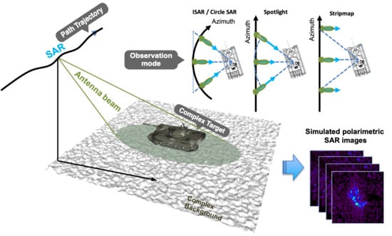
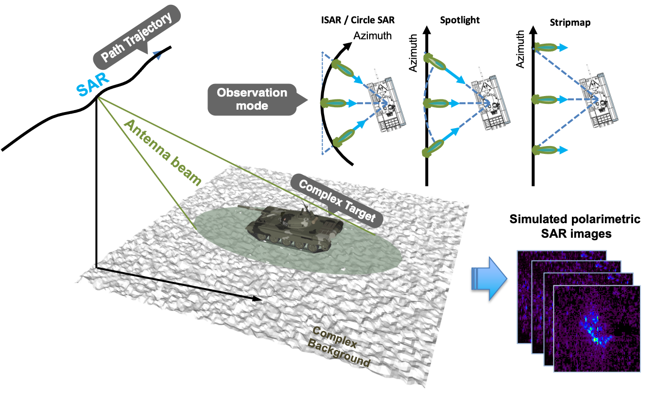
From the above reviews, it is clear that there is a need for an efficient SAR signal and image simulator, including the SAR echo signal generation considering the coherent integration of the target and background. This simulator can also simulate incident wave rays and the propagation into the inter- and intra-interactions of targets and background clutter. The clutter and speckle are coherently given. Besides, the SAR geometry can be flexible to accommodate different SAR acquisition modes under sensor path trajectory variations. This paper aims to coherently integrate all the signal chains, starting from radar signal transmission to final image focusing, emphasizing the fast computation of the multi-frequency backscattering field in the course of synthesis aperture imaging.
In the next section, we briefly introduce the SAR signal model to facilitate the fast computation algorithm implementation in
Section 3. An accumulated speedup table is summarized to validate the performance of parallel computation.
Section 4 illustrates a model-based SAR simulation of the MSTAR-like 3D CAD model and multiple target’s aspect angles. Finally, we provide a summary of the SAR simulation with a high parallelization performance to close the paper.
3. Computation of SAR Backscattering Field
3.1. An Iterative Shooting Bouncing Ray
In Shooting Bouncing Ray (SBR) [
20], geometric optics (GO) is utilized to describe the electric field direction and energy propagation into and away from the target being imaged. We use the bounding volume hierarchy (BVH) method [
21] to build the 3D target model. In general, the target surface is curved.
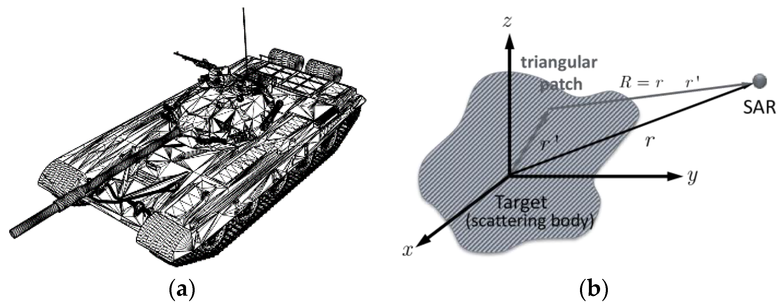
Figure 4a displays a 3D CAD model of the T72 tank. When imaging by SAR, the incident and scattered waves into the target and out of it are complex; together with BVH in SBR, we can determine which triangle patch is inter-sectioned by the specific ray using a fast ray-box intersection algorithm. The intersection point on this triangle patch and the reflection vector can be calculated from Snell’s law. The number of bouncings is iteratively determined according to the target’s geometry complexity until preselected criteria are met. The target can be multi-layered dielectric coatings on PEC or pure dielectric, for example.
By including multiple bounces, Equation (1) can be rewritten as a coherent sum of every single bounce (
):
where
I is the slant range from the target’s origin to the sensor’s instantaneous position;
is the relative slant range of the target’s origin and the
k-th intersection point on the target for the ray-racing technique; and
. The field
is the scattering electric field of the
m-th bounce;
stands for the component of the scattering electric field in the
k-th ray of the
N, the number of the rays tracing determined by SBR [
20]. In computing Equation (5), we assume the “stop-and-go” SAR signal model [
19]. The amplitude of the electric field weakens with an increasing number of bouncing. In what follows, we shall detail the SBR in the context of SAR imaging using Equation (2) as a working model to generate the received signal or the SAR raw data.
In the incident surface, the spherical surface is needed to satisfy the requirement of the near and far field conditions. The smallest cell size,
, on which the wave incidences and is determined by
, where
is the distance from the pseudo origin of the spherical surface to the shell of this sphere; and the
relative to the smallest angle,
, should be at least less than one-sixth of the radar wavelength [
8]. By this, the minimal spanning angle of this incident surface grid in the vertical and horizontal directions is calculated by the eight projection points of embracing hexahedron projection on the incident surface following the ways shown in
Figure 3. Based on the spanning angle and direction, the two tangential unit vectors and minimum sizes of the grid cells are determined.
3.1.1. Electric Field in Sphere Coordinate
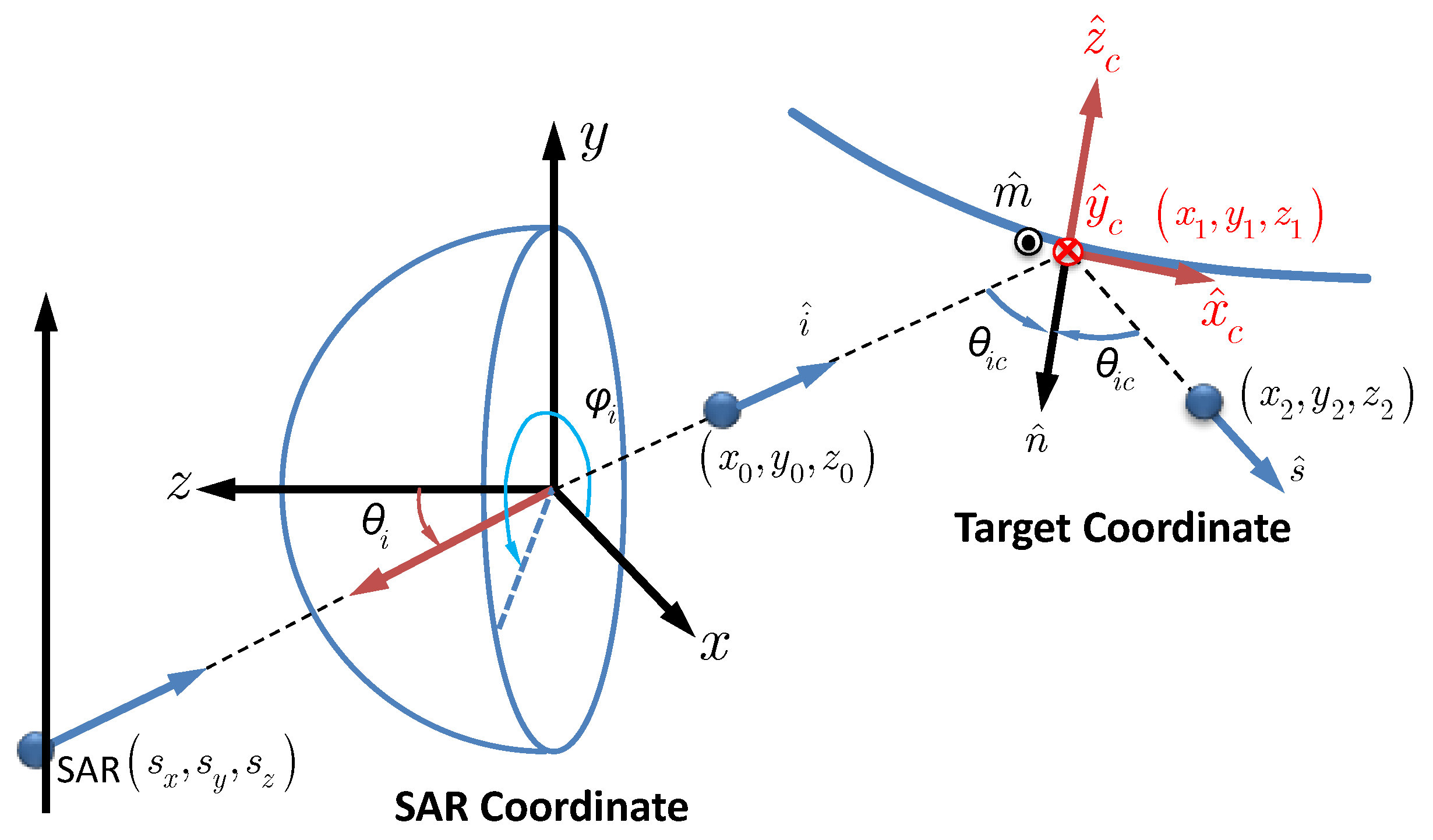
Referring to
Figure 5, at the SAR sensor coordinate, the origin of the incident electric field is
, with the instantaneous incident electric field at
, with
and
representing the radar incident angle and azimuth angles, respectively. The incident field impinges upon the target’s surface
at target coordinate
with the local incident angle
. The target coordinate is defined by both the incident vector
and the target’s surface normal vector
:
where
is the unit vector perpendicular to the target’s surface,
. It follows that the local incident angle
can be found as:
From the Snell’s law, the reflection direction can be readily obtained.
3.1.2. Coordinate Transformation
At this point, we need to transform each patch from the local coordinate to the global coordinate. Referring to
Figure 6, the transformation between the global coordinate and the local patch coordinate is by matrix [
1,
22]:
where:
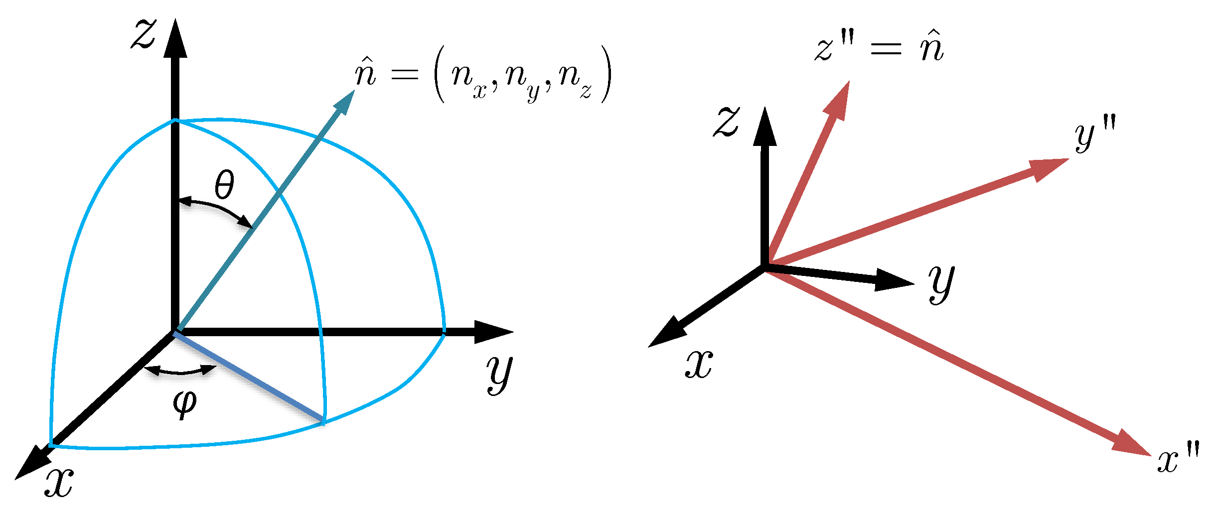
where the azimuth and polar angles are
, with
being the unit normal vector
, where
is always one.
3.2. Surface Current Density and Scattered Field
The far-field scattered field due to the surface current density:
where
A is the illuminated area,
is the intrinsic impedance, and
is the project length from
to
. The surface current sources come from the electric current density
and magnetic current density
.
Once the surface current density is known, the scattered field can be calculated. Numerous fast computation algorithms have been proposed in the frequency domain or time domain [
23]. Although the solutions may be accurate, they are still computationally prohibitive for an electrically large and complex target for SAR image simulation. As we already saw from Equation (1), the scattered field must be repeatedly calculated when SAR moves because the incident wave direction changes. If we further consider the target orientation to build a complete SAR image database, the computation of the scattered fields would stall, if not stop, the simulation.
For the target under consideration, we assume each patch has a tangent plane such that physical optics (PO) approximation can be applied to obtain the surface current density
,
in the illuminated region:
where
and
are the Fresnel reflection coefficients for vertical and horizontal polarizations, respectively;
and
where
are the p-polarized incident electric and magnetic fields, respectively. For a perfectly electric conducting (PEC) target,
and
. For multi-layered dielectric targets, the reflection coefficients can be calculated by a recursive formula given in [
24].
Under the PO approximation, the scattered is denoted by
. The scattering is from the local tangent planes from every patch and the wedges in a triangular patch. We use the physical theory of diffraction (PTD) to include the diffraction field produced by the fringe current at or near edges. The diffraction currents on the dielectric edges are given by [
25]:
where
is the unit vector tangent to the edge,
is the angle between the edge and the incident or diffracted direction,
is the angle between the incident direction and the top surface of the wedge,
and
are the corrections for the reflection coefficients of the surfaces that form the wedge given in [
25], and
are the Ufimtsev’s diffraction coefficients for the Keller’s cone case [
26]. The diffracted field due to the diffracted currents given by Equations (15) and (16) is [
26]:
where
is the distance from an element on the contour
C to the observation point, and
is the differential length along the edge discontinuity length
. The diffracted field
is the correction to
such that the total estimated scattered field is:
The scattered field given in Equation (18) is in global coordinate and is transformed to local coordinate through Equation (9) before being substituted into Equation (4) for an instantaneous azimuth position. Computations continue as SAR is imaging the targets during the aperture time. It is not difficult to realize that the calculation of scattered fields is heavily burdened for various SAR acquisition modes. Furthermore, the raw signal is repeatedly generated by Equation (4) for each step of receiving the scattered field.
3.3. Computation Parallelization
In the processing flow using Equation (6), computing the scattered field for each SAR azimuth position poses the highest complexity in terms of computational parallelization. The computing time complexity is , where is the required number of bounces, and is the equivalent number of ray beams, frequencies, and aspect angles; in common practice, is easily at least on the order of 109. Our goal is to reduce the overall time complexity to , if proper optimization is attempted and implemented. The most massive loading stems are from the inner loop of calculating the scattering electric field by integrating the surface current, governed by the integral equations, for each incident ray impinging upon the target. Inside the integration, the coordinate transformations between global and local coordinate systems are involved. Hence, to this end, the parallelization scheme based on NVIDIA CUDA includes several components described below.
We carried out the computation of scattered fields in the frequency domain for range compression. The outer loop is the essential ray-tracing element for each grid on the different incident surface mesh. The initialization of shooting and bouncing variables is declared here. The multi-frequency is involved in the next loop because the transmitted signal and scattered signal are frequency dependent with the fast ray-polygon intersection algorithm, which has the time complexity of . The inner loop treading the bouncing process can be divided into five steps.
SBRs: We conduct the ray tracing in the outer loop and extract the information of the intersection point and the reflection direction.
Pre-calculation: We calculate and store the distance between the current and previous bouncing points, local coordinate transformation angle on the intersection polygon, and global coordinate transformation matrix in the cache of GPU.
Dielectric grid: We compute the reflection coefficients for the dielectric target for each grid on the incident ray’s target.
Post-calculation: We conduct the ray beam area normalization and wave propagation distance in this step. The parallel and perpendicular electric field components must be projected onto the receiving plane using the relationship of the geometry matrix of the scattering field and the receiving plane in the pre-calculation given in step 2.
Summation: We sum up the scattered fields for all frequency components at a certain SAR look angle and the target’s aspect angle, using the CUDA parallel reduction algorithm.
As illustrated in
Table 2, in terms of the computation complexity for general SAR acquisition, the aspect angles are 10 to the power of 3. The ray-tracing elements are on the order of 10 to the 10 to the 7 power, the frequency steps can be 10 to the 10 to the 2–3 power, and the iteration number of multi-bouncing is between 1~10. This ends up with the overall time complexity
. Comparatively, the number of bounces,
, is small compared to
represented by
,
, and
.
Table 3 gives the computation environment, and
Table 4 summarizes the cumulative speed up compared to the sequential coding (no paralleling implementation). The breakdowns clearly show the time distributions of each stage of operation. The overall speedup factor is up to 224
. This speedup, however, does not imply a limit. Using higher specifications of GPU and enhancing parallel optimization would be able to push up the speedup.
4. Validations
We used canonical targets of the sphere and the dihedral reflectors to validate the simulation. The sensor parameters and the associated imaging parameters are listed in
Table 5. The radar frequency was set to 9.6 GHz with 591 MHz of bandwidth, and four polarizations of HH, VH, HV, and VV were simulated. The path trajectory length means the SAR moving distance with a look angle of 72.64°. Using this setup, the range of the azimuthal scanning angles was relatively small, about 3.9°. For SAR data takes, we computed the backscattering field at a small step of 0.003362. We adopted the “stop-and-go” model in the simulation, so the phase ambiguity problem mainly occurs in the azimuth direction, especially in the Doppler centroid estimation. For a zero-squint, the phase ambiguity is not an issue. For a squint angle of 30 degrees, the ambiguity number is larger than one PRF. Nevertheless, we were able to obtain a reasonable estimate of the Doppler centroid frequency. We implemented a Range-Doppler algorithm (RDA) for Stripmap mode and an Omega-K algorithm (WKA) for Stoplight mode for image focusing [
19]. The multi-looking cross-correlation algorithm (MLCC) and the multi-looking beat frequency algorithm (MLBF) were used to estimate the phase ambiguity.
The computations of the backscattered field during aperture synthesis are required to apply Equation (6) to obtain the SAR signal, a complex signal. Computationally, every single ray bouncing can be recorded and processed into the SAR signal. In dealing with the iterative computation of ray bouncing in Equation (6), we continued the ray tracing until the multiple scattered field amplitudes:
where
m is
mth ray bouncing as indicated in Equation (6). The convergent rate depends on the geometry complexity and dielectrics of the target. In such a way, we can better explore the scattering process and its dependence on radar and target parameters, both dielectric and geometric.
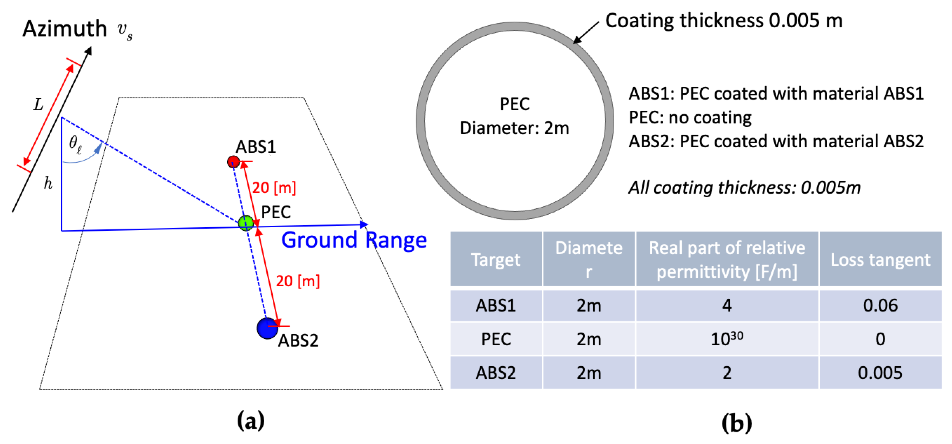
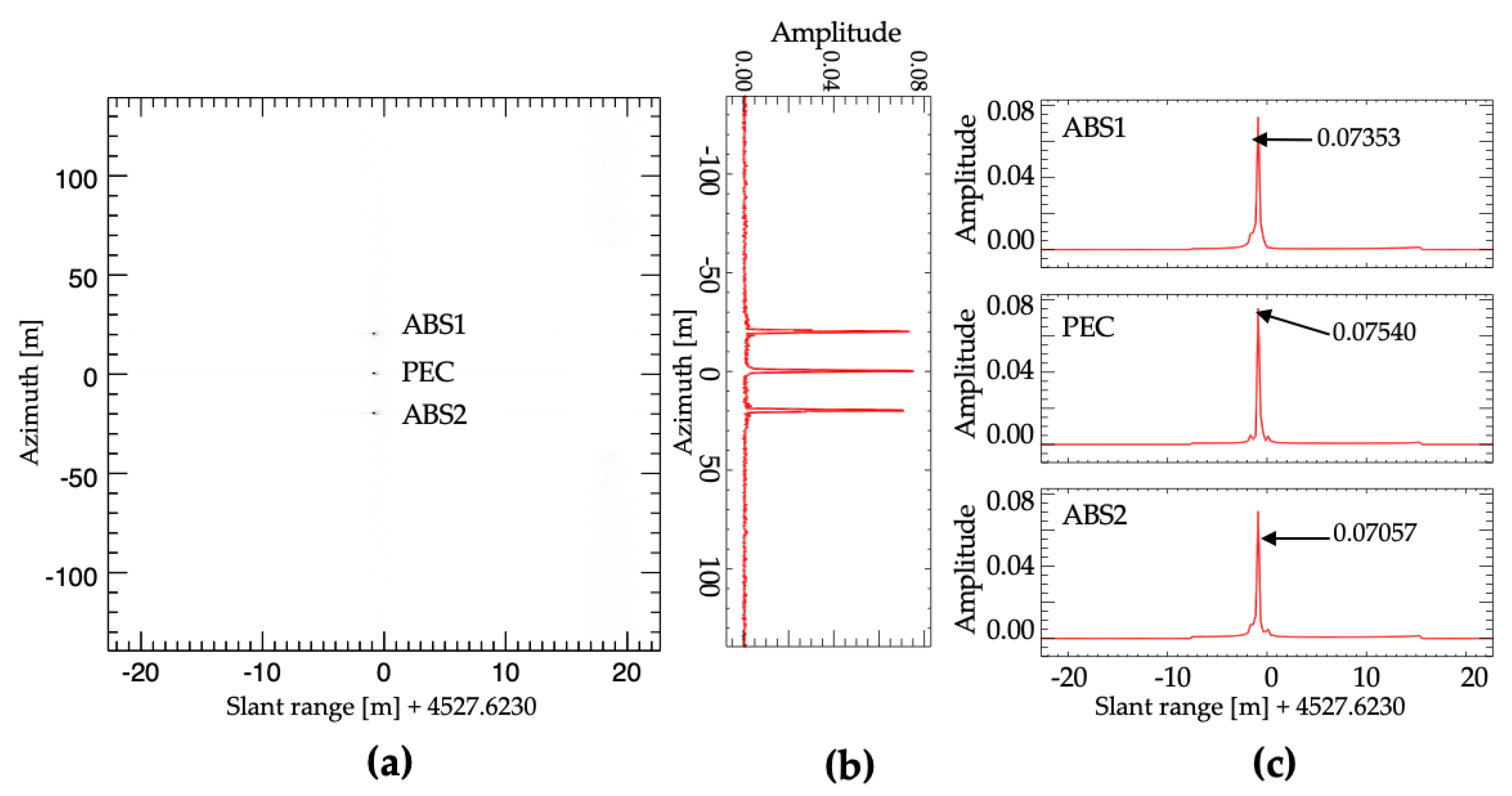
We begin simulating the sphere target; the scene consists of three spheres: a PEC and two dielectrics coated on PEC spheres. The coatings had a thickness of 0.005 m ABS1, PEC, and ABS2 coating, placed along the azimuth direction spaced uniformly 10 m apart, as indicated in
Figure 7a. The diameters and dielectrics of the three spheres are given in
Figure 7b. For a further inspection, we illustrate the amplitude responses of the azimuthal and range profiles for three targets in
Figure 8b,c, respectively, which are all cut through the focused images’ peak values in
Figure 8a. Rich information can be revealed due to electromagnetic wave behavior, such as scattering and penetration, occurring concurrently. In the ABS2 target with the lower dielectric constant, much of the power penetrates through the media. Thus, the first response is weaker than the PEC target, whereas the boundary reflection occurs with a small response. With an increase in the dielectric constant, the first response of the ABS1 becomes stronger, and the penetration energy decreases.
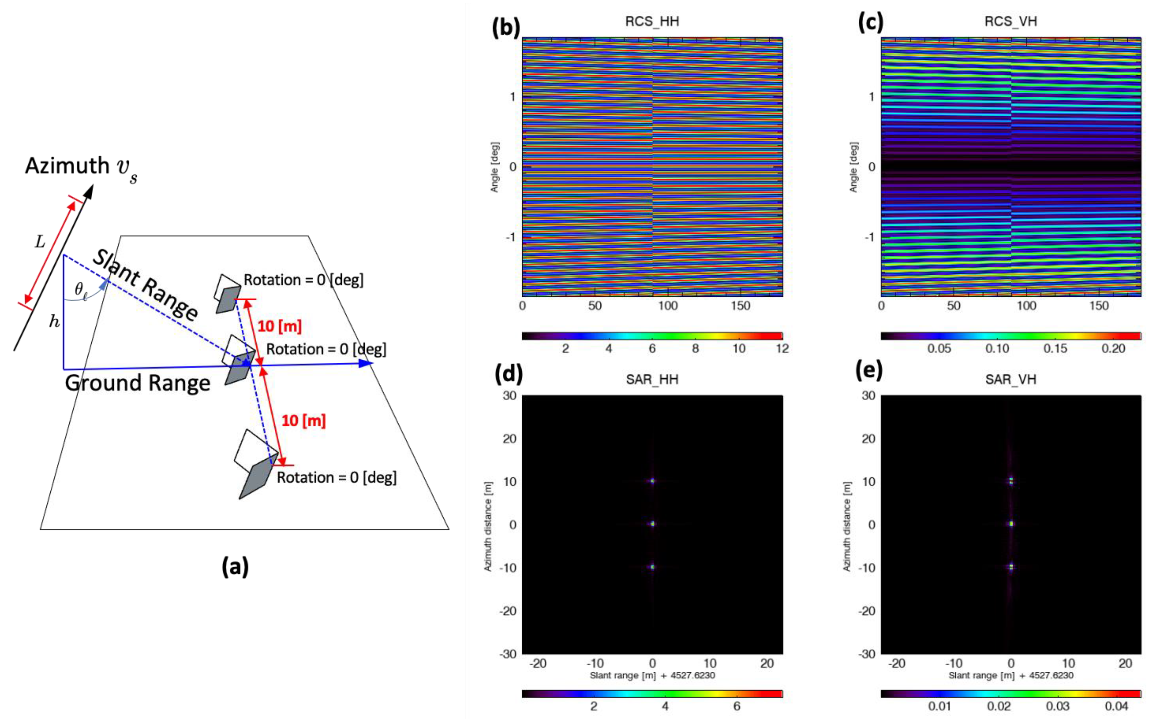
The canonical targets of the sphere and the dihedral reflectors, with their known scattering matrices, provide ideal targets of polarimetric calibration and polarimetric image focusing, both qualitatively and quantitively.
Figure 9 illustrates the image scene, similar to
Figure 7a.
Figure 9b shows HH and VH polarized RCS and the dihedral reflector RCS variation with the illumination angle, for the azimuth angles of interest. The focused HH and VH polarized images are illustrated in
Figure 9d,e, respectively. Three dihedral reflectors are identified in the HH polarized image, whereas the VH polarized image itself can appear due to the angle dependency and edge effect of the dihedral reflectors. The HH polarized image is approximately 22 dB stronger than the VH polarized image in
Figure 9b. The dominant scattering of a dihedral reflector is double-bounce scattering in the HH image. In a deeper inspection of the VH polarized image, the two dihedral reflectors placed at 10 m apart exhibited their shapes in two parts. This corresponds to the VH polarized RCS return in the azimuth-frequency domain, where the VH polarized RCS is more dependent on the azimuth angle. The VH polarized RCS will be enhanced when the sensor scans away from the dihedral reflectors due to the absence of the azimuthal reflection symmetry.
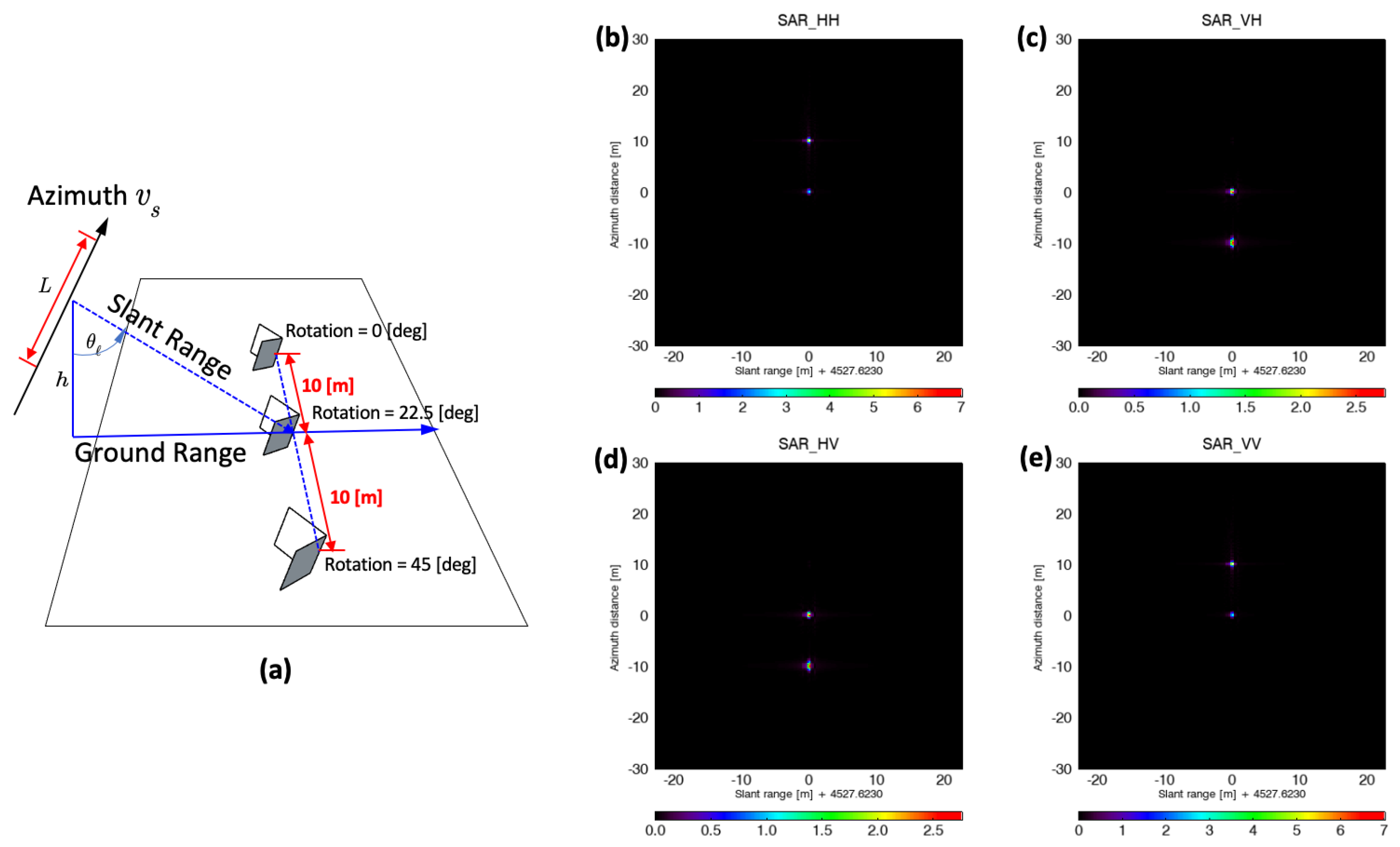
In the third simulation case, the three dihedral reflectors have different orientations by rotating 0°, 22.5°, and 45°, placed along the azimuth direction with the spacing of 10 m.
Figure 10a illustrates the imaging scene, while
Figure 10b–e display the fully polarized focused images with HH, VH, HV, and VV respectively. We may identify the 0°-rotated dihedral reflector in the HH and VV polarized images, as is the 45°-rotated dihedral reflector in the HV and VH polarized images. We can also observe the 22.5°-rotated dihedral reflector in the fully polarized images, which agree with the theoretical scattering matrices [
27].
5. Examples of Simulation Images of a Complex Target
The complex targets with high structural and interaction between the target and background were presented in a section later without loss of reliability. The MSTAR dataset is a highly representative example that corresponds to our purpose flow chain to simulate a dataset. We applied this simulator to the MSTAR T72 target. The real SAR image had 1 feet resolution by the Spotlight SAR acquisition mode in the airborne system, operating at X band with high depression angle 15° and 17°.
5.1. Target CAD and Observation Setup
The target’s type in the public dataset has more than 10 kinds, and there are up to almost 300 different aspect angles for each target. Because of the high acquisition look angle, we could find the shadow effect easily in the images dataset. The 3D CAD model was Autodesk 3DS Max file format with 1,086,030 polygons that triangulates from the original model [
28]. The model is placed on the plane ground to examine the multi-bounce effect due to the ground surface. The aspect angles were within [−1.8502, 1.8468], with an interval of 0.0033 degrees to match the PRF of 213.4 Hz, ending with 1100 samples. We adopted the sensor path trajectory with a general XYZ coordinate at an equal sensor height, and all light-of-sight was projected onto the geodetic coordinate with WGS84 datum. Because the target includes the background in the square 20 m area, we restricted the maximum observation swath to 95.6 m, resulting in 360 samples, such that the spacing was 0.2536 m.
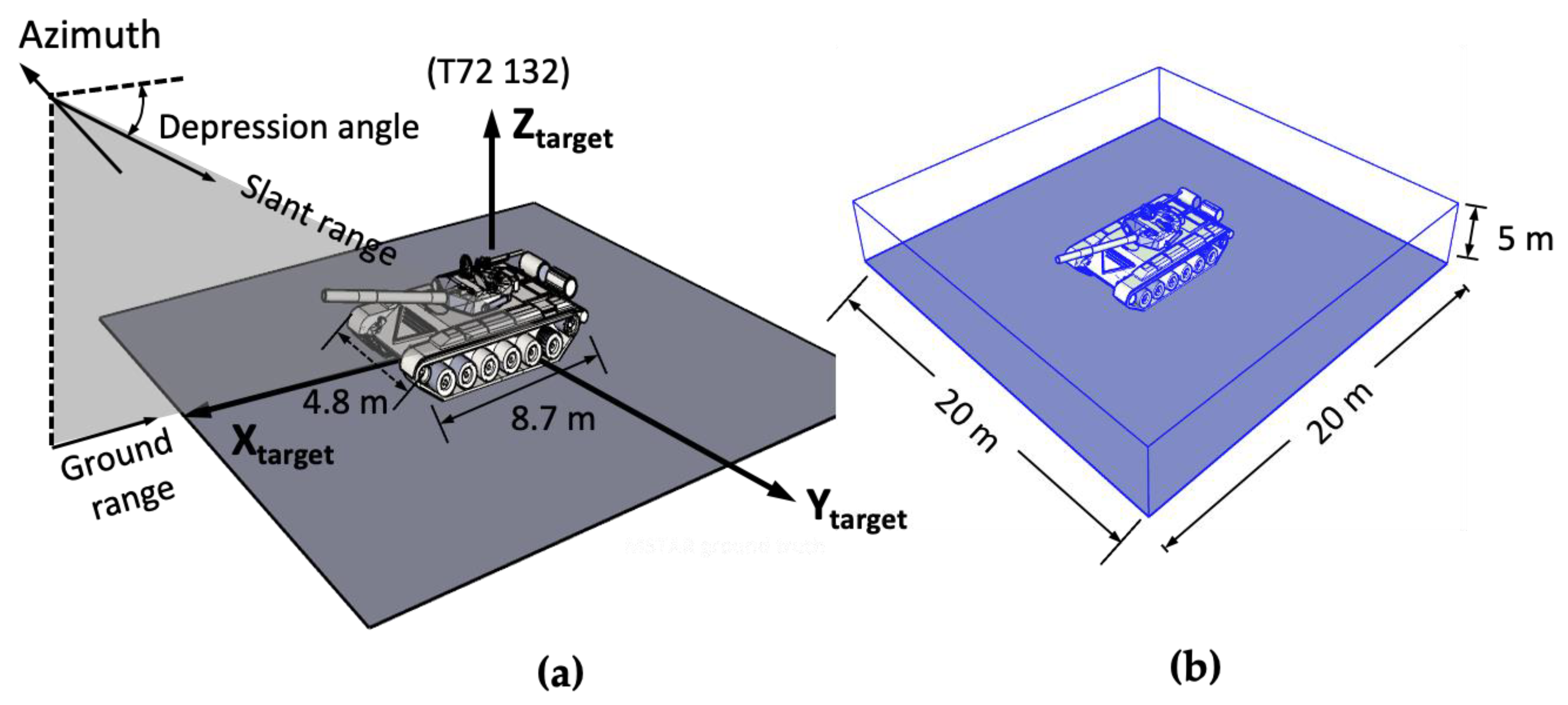
Figure 11 shows the surrounding box with a 20 m square and 5 m height for covering the background and target.
Figure 11a shows the SAR sensor using Spotlight acquisition mode directs to the target with a depression angle. A pseudo ground plane was added to the model for the double-bounding effects between the ground and the wheels. To implement the SBR, we applied an embracing bounding box for a fast ray-triangle intersection, as shown in
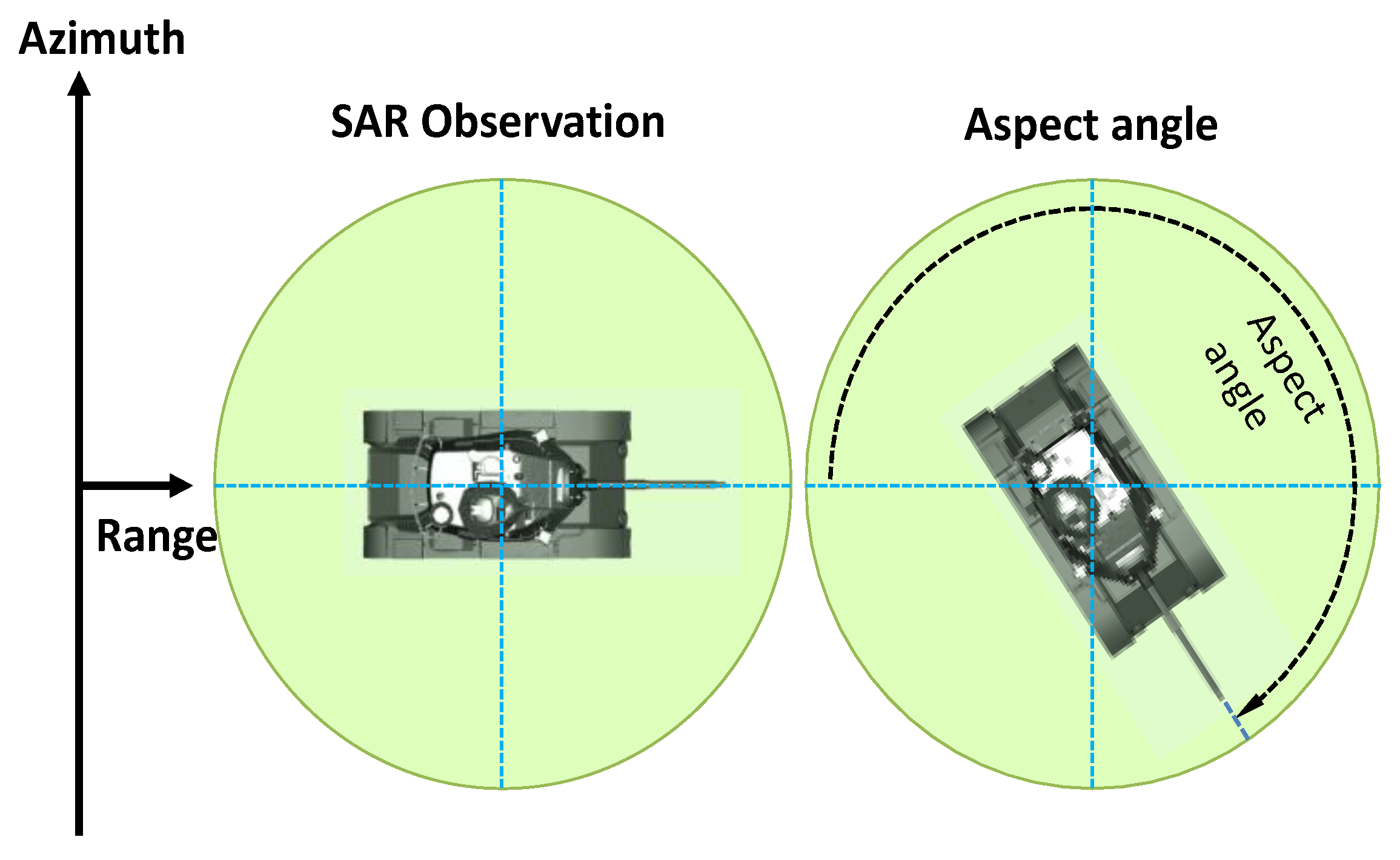
Figure 11b. The SAR image features are sensitive to the relative orientation; different aspect angles are included in the simulation dataset. The aspect angle is defined as the line of sight pointing to the right (see
Figure 12). The aspect angle is rotated along the
z-axis with the left-hand rule that is the same as the MSTAR dataset.
5.2. Simulation Parameters
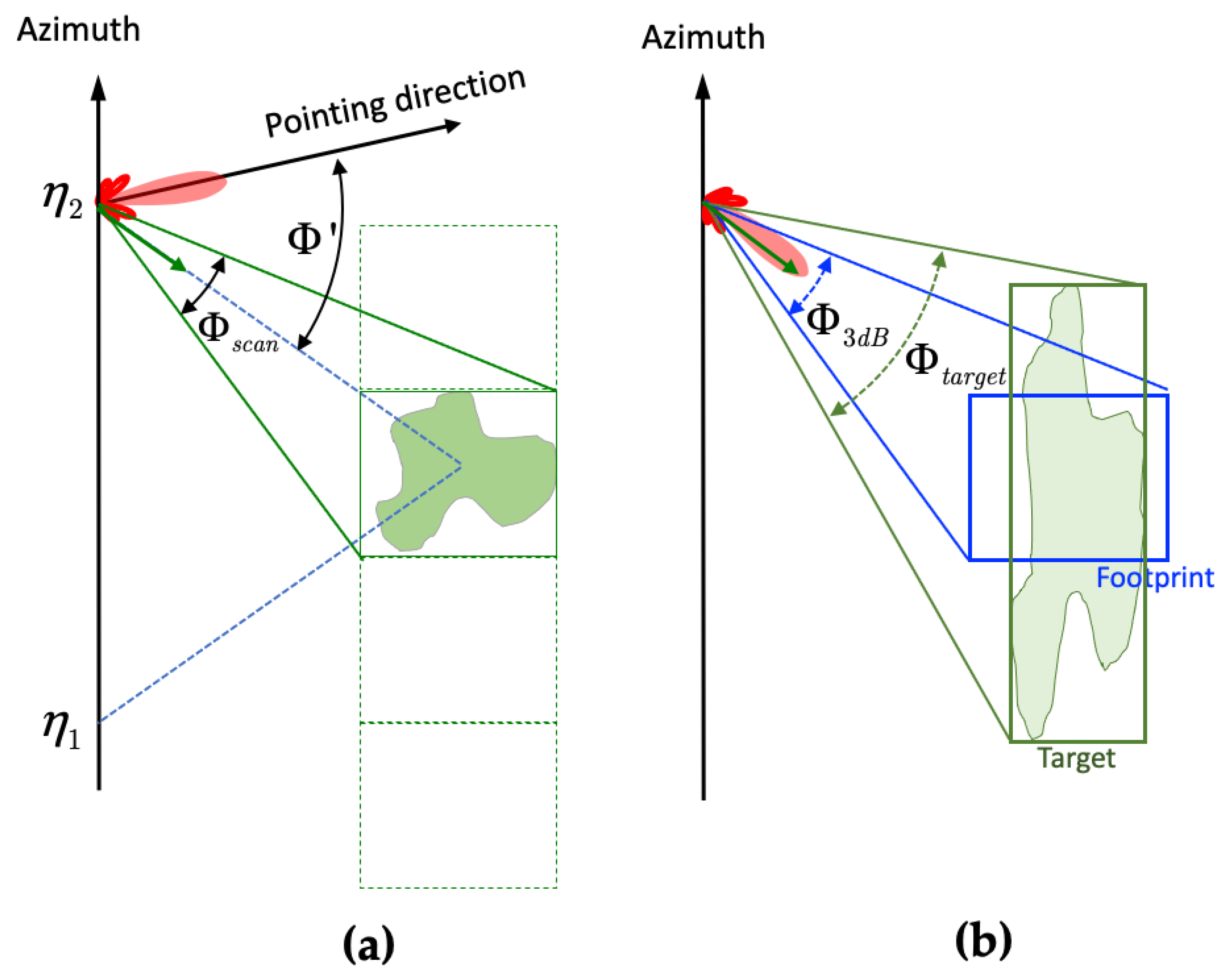
Table 6 summarizes the simulation parameters. To be consistent with the MSTAR specifications, we used the X-band with a 9.6 GHz center frequency, 591 MHz bandwidth, and HH polarization. We calculated the antenna beamwidth, range resolution, and spacing from the effective antenna length. Note that the state vector’s position and tangential velocity can be derived from the azimuth dimension and PRF. The Doppler parameters in
Table 7, including the Doppler bandwidth and rate, were calculated using the antenna beamwidth and PRF. The spacing at both directions was set to almost 0.25 m to meet the 1 feet resolution requirement in real MSTAR data [
29]. The scan angle range was calculated by Equation (3). The image size was 360 samples of frequency sampling in the range direction and 1100 samples of azimuth sampling for fully azimuth synthesis.
5.3. Simulated Images and Discussions
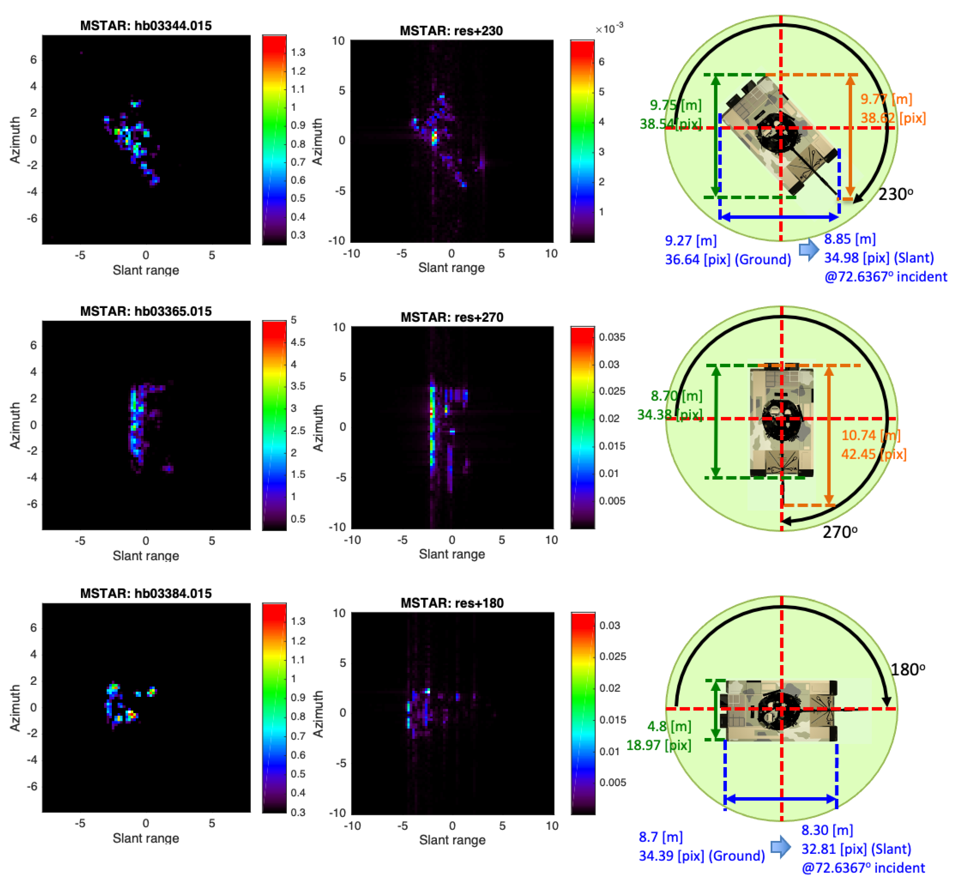
Figure 13 compares real and simulated images at 230°, 270°, and 180° aspect angles. The left column is the MSTAR actual image in amplitude. The simulated SAR amplitude images are in the middle, corresponding to the relative target’s geometry, including the target’s attitude and the slant and ground plane’s dimension. We note that the barrel pointing direction was different: the barrel direction aligned with the vehicle body in the simulated image but was slightly offset, appearing in the real image with an unknown angle. For example, in the 230° aspect angle, the maximum dimension at azimuth is 9.77 m or about 38 pixels. The slant range is 8.85 m, corresponding to about 35 pixels, and at the ground, the range is 9.27 m, nearly 36 pixels. From these high-resolution simulated images, we found the structure of the turret in the 230° clip. The double bouncing effect with strong scatter mainly occurs. In the 270°, the strong single and double bouncing induced by the wheels and track was shown along the azimuth direction. The barrel structure is also present here because the pointing is perpendicular to the line of sight. The two secondary fuel tank structures can also be found in the 180° clip because they are the first intersection targets with the radar incident wave.
At this point, it is worth noting that the main factor most likely to produce the high levels of sidelobe, as shown in the simulated images of
Figure 9 and
Figure 13, is due to the antenna 3 dB wide range. To speed up the echo signal generation, we limited the exposure range of the antenna, as indicated in
Figure 3, to alleviate the computation burden. This exposure time gives rise to a
sinc squared-like function to reduce the edge effect, but considerable sidelobes still appeared after image focusing. In our SAR imaging simulation, we applied a Kaiser window in the azimuth direction. We may suppress the sidelobe level in our future work by (1) expanding the physical range of the antenna gain pattern in the echo signal generation process, (2) enhancing the azimuth window filtering in the SAR imaging process, and (3) increasing the azimuth window filtering in the SAR imaging process. Methods, such as spatially variant apodization and sparsity constraint regularization, may be applied. We will attempt to implement them in our future simulations.
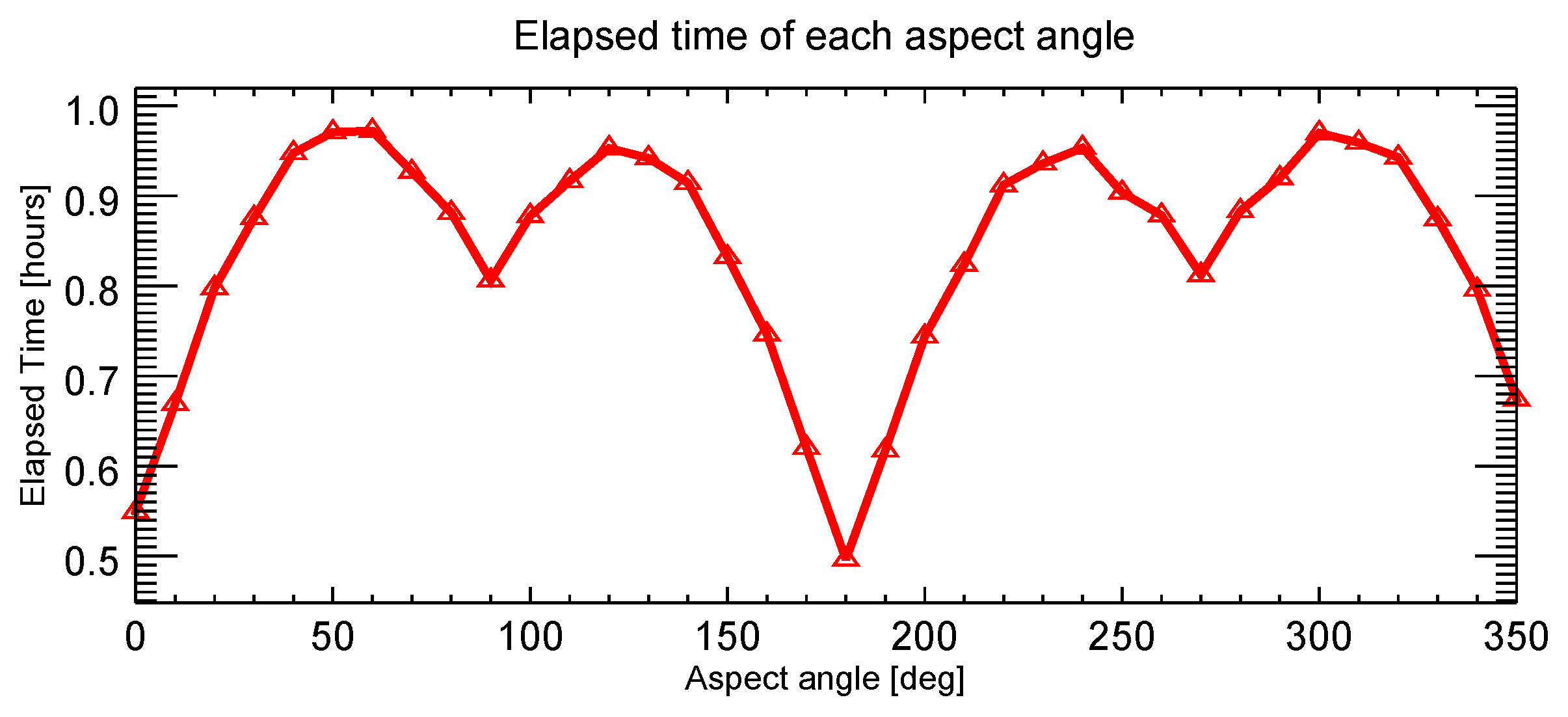
Figure 14 shows the GPU computation time corresponding to every aspect angle, where the calculation time is dependent on the target’s pose to SAR observation. We can note a symmetry of about 180° of the aspect angle. A longer computation time was required to reach convergence in accounting for the multiple bounces in ray tracing, implying in some sense that richer image features about the target may be acquired.
Table 8 shows the two extremes, the longest and shortest computation times at the 60° and 180° aspect angles.
The image size is 360 samples of frequency sampling and 1100 samples of azimuth sampling; it took 43 and 74 h of CPU computation time. The GPU-based algorithm proposed in this paper reduces the computation time to less than an hour, with a speedup rate of more than 70 times. Compared to the 224
speedup shown in
Table 4, we note that for a much more complex target than in this example, the rays in SBR may go through quite different bouncing numbers. So, there will be many threads waiting for the one that takes care of the highest number of bouncing when executed simultaneously on the GPU thread. Nonetheless, the proposed GPU-based parallel algorithm offers an effective and efficient approach to simulating the SAR image of both complex geometry and electrically large targets, such as the T72 tank demonstrated in this example. This allows us to build up more complete simulated SAR images for target poses for classification and identification.
As mentioned previously, the total bouncing from the incidence to the scattering out of the target can be decomposed into individual bouncing. The scattering signal from this individual bouncing can be processed into SAR images so that the detailed interaction of the scattering process can be extracted to explore the target features.
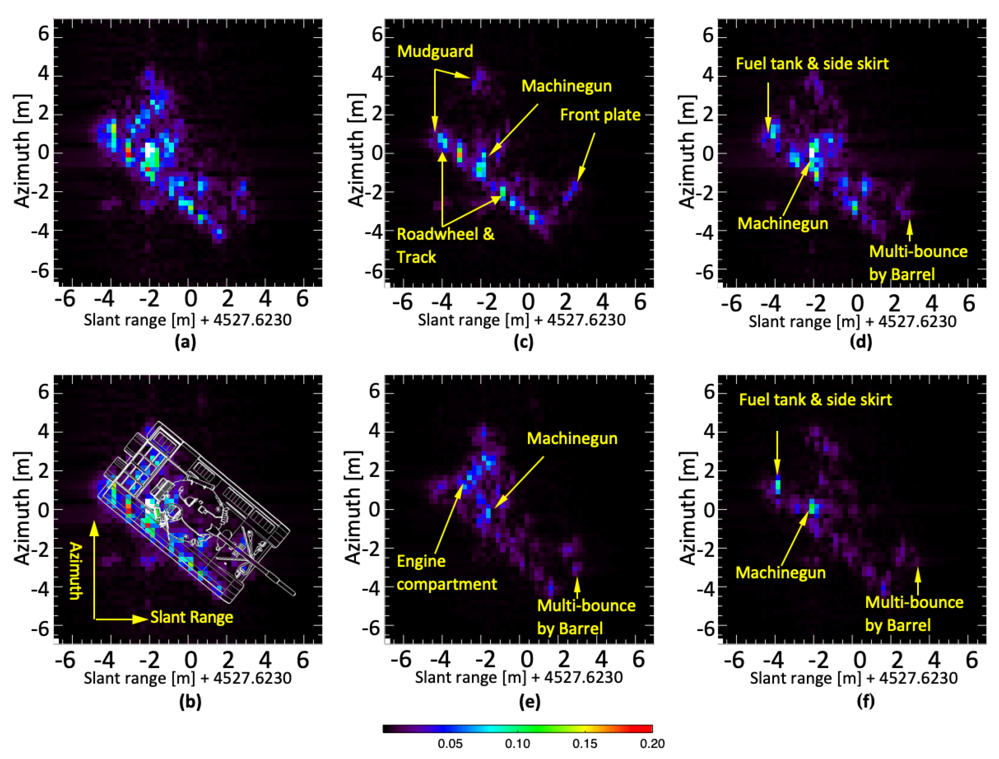
Figure 15 shows the total bouncing image after a coherent sum of the individual bouncing signal at a 220° aspect angle. To better visually inspect the image feature, we also overlaid the target’s wireframe on the
Figure 15a image, as shown in
Figure 15b.
Figure 15c–f display the simulated images from bouncing 1 to bouncing 4, denoted as level 1 to level 4. Because the signal level decreases with the increasing number of bouncing, for comparison, we normalized the image amplitude to a maximum value of 0.2. At levels higher than four bouncings, the signal is too weak and is not shown.
A further look reveals that the strong scattering points between the roadwheel and trace appear in level 1 and level 2 images. The structure between the roadwheel and trace is involved but is also significant for enhancement of the wave scattering. A strong scattering phenomenon also appears in level 3 and level 4 images but with much weaker intensity. The machinegun position feature is visible in level 1 through to level 4 images and is most apparent at level 2. Because, at this pose, the machinegun placement is parallel to azimuth and is located on the turret side, it is a scattering preference. In the level 2 image, there is significant scattering at the junction of the secondary fuel tank and side skirt, considered a Dihedral-like reflection, and this is not presented in other level images. The engine compartment that appears in the level 3 image has a regular pattern across the slant range. The cooling plate produced regular patterns, which is mainly due to the contribution from level 3 after decomposition. The mudguard and side skirt features, which make up one of the most distinctive features of this target, appear at the close range but disappear as the turret is obscured at a far range due to the shadowing effect. There is a distinct feature point at the barrel and front plate junction, which gradually moves toward the far range from level 2 to level 4 due to multiple scatterings between the barrel and front plate. As the number of bouncing (higher levels) increases, the wave travel path becomes longer so that the scattering point gradually moves toward the far range.
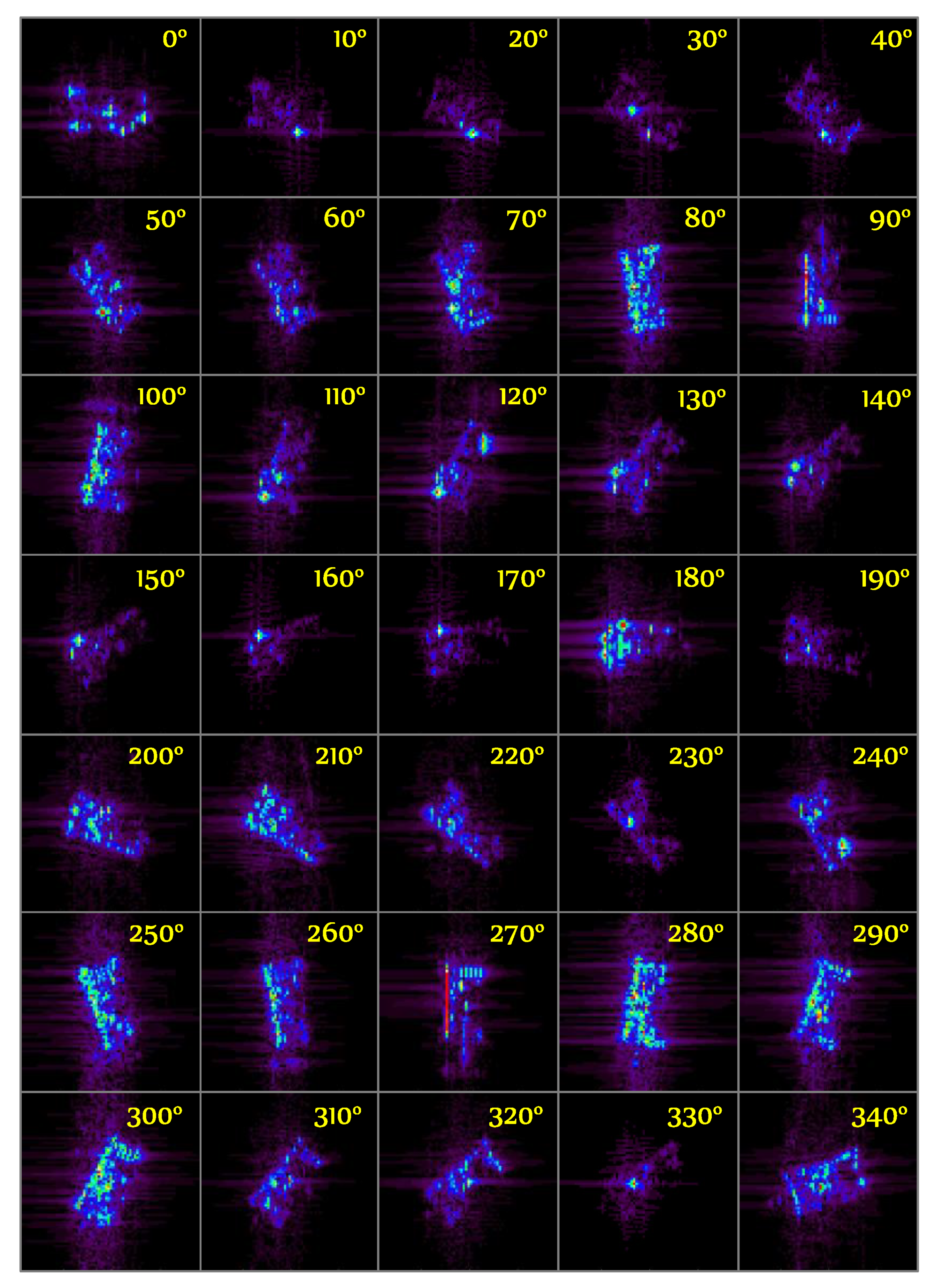
Finally, we simulated the T72 target dataset covering the aspect angles simulated from 0° to 359° with a step of 1°.
Figure 16 displays 35 clips for a step of 10° of the aspect angle. With such high-resolution images, the image features are quite different from various angles, which is no surprise since the SAR is sensitive to the target’s poses relative to the sensor. From the image set, we can only see the gun structure at angles of 90° and 180°. Some persistent structures of the targets nevertheless show up in the simulated images.
6. Conclusions
We proposed a GPU-based fast computation of multiple scattering to simulate the SAR image in a coherent system approach. For computing the backscattered fields, we adopted the shooting bouncing ray (SBR), the physical optics (PO), and the physical theory of the diffraction method. To be more realistic, we included the antenna pattern tracking to generate the SAR echo signal. The SAR acquisition mode can be Stripmap or Spotlight. The implementation of the computation parallelization of SAR echo signal generation was demonstrated. By profiling, the overall processing was identified to find which is the heavy loading stage. A dedicated hardware orientation language, NVIDIA CUDA, was adopted. To accommodate the hardware structure, we devised extensive modifications in the CUDA kernel function. We used a GPU card to evaluate the performance of the speedup rate for each modification. Moreover, the accumulated speedup rate was shown in the experiment tables. As a result, the speedup is very high, with over 224 times speedup rate. The computation complexity was demonstrated by comparing the CPU and GPU computations. As a coherent SAR simulator, we included the following chains: SAR returns signal model from targets, whether simple or complex, the range frequency sampling to create the range bin profile, the sensor path trajectory with motion including system error and random noise, the geometry relation between the SAR observation and target, and, finally, image focusing. We then validated the proposed simulation algorithm, using PEC and dielectric spheres, and rotated/unrotated dihedral corner reflectors. We showed that the simulated images by the proposed method have high fidelity in their geometric and radiometric qualities. In particular, the simulator can preserve the polarimetric information of the targets. As an extensive image features database is essential for target detection, identification, and recognition from the SAR image, the fast simulation architecture proposed in this paper fully meets this demand. We will further refine the algorithm to speed up the computation and include other SAR acquisition modes, such as circular SAR and inverse SAR.


