Sub-Bottom Sediment Classification Using Reliable Instantaneous Frequency Calculation and Relaxation Time Estimation

Abstract

The shift in IF (instantaneous frequency) series and the corresponding relaxation time have the potential to characterize sediment properties. However, these attributes derived from SBP (sub-bottom profiler) data are seldom used for offshore site investigations because of the unsoundness in attribute calculation. To overcome this problem, a new reliable method combining VMD (variational mode decomposition) and WVD (Wigner–Ville distribution), as well as relaxation time, is presented. Since the number of modes in classical VMD should be provided in advance, a modified VMD algorithm, MVMD (modified variational mode decomposition), is proposed here, where the distribution of the frequency domain of modes is taken into account to automatically determine the number of modes. Through the relaxation time model, the IF data of a series of pings calculated through MVMD-WVD are transformed into a relaxation time map. A robust estimation algorithm is applied to the relaxation time map to reduce the effects of interferences and obtain robust relaxation times. The final relaxation time data are used to determine the sediment types. Real data from SBP experiments, as well as borehole sampling and geotechnical analysis results, verified the good performance of the proposed method.

1. Introduction

SBPs are designed to image the underwater sub-bottom sediments for mineral resource exploration, marine scientific research, and so on [1,2,3]. In one ping measurement, the SBP transducer transmits acoustic waves and then receives reflected echoes. The recorded sequential echoes reflect the structural information of the measured sediment layers, and the reflection strength and IF of SBP data may aid in the lithology identification of sub-bottom layers [1,2,3,4,5,6,7]. Remote sediment classification based on SBP data enables the sub-bottom to be mapped more quantitatively, thus improving the degree of confidence of geological predictions, and this in turn has the potential to decrease the reliance on costly seabed sampling. However, the existing use of SBP is still mostly limited to the delineation of stratigraphic structures, although the remote acoustic classification of the physical properties (reflection coefficient, attenuation coefficient, etc.) of shallow sediments is of paramount interest to the geotechnical and geological communities in the field of mining and exploration for placer deposits and other marine mineral resources [4,5,6,7,8,9]. For example, SBP sediment classification based on the data acquired by De Beers Marine helped its offshore mining and exploration programs for diamondiferous placer deposits, situated on the continental shelf off the west coast of South Africa [9].

Sediment classes are still difficult to obtain because of unsoundness in acoustic attribute estimation [9]. To deal with this problem and improve the classification potential of SBP data, there are many researchers who have made efforts in this field using different methods [10]. These methods can be divided into three categories: reflection coefficient-based methods, attenuation property-based methods, and machine learning methods.

Mohamed [11] proposed an algorithm that estimates the reflection coefficients of layers on the basis of signal energy reflected from various interfaces to achieve sediment classification. They derived the multilayer acoustic energy equations and estimated the reflection coefficient of every sediment interface. Plets et al. [12,13] also used the reflection coefficient to analyze the properties of sub-bottom sediments, which is rather simple and practical. They calculated the reflection coefficient as the ratio of the amplitude of the reflected wave and the amplitude of the incident wave. However, in sub-bottom applications, attempts to obtain reflection coefficients are still limited. The analysis window size in Mohamed’s method can result in unsoundness, while Plets’s method can be invalid if no multiple exists.

Because of the higher frequencies used, as in the case of sub-bottom imaging, attenuation significantly alters the reflection response. Thus, the attenuation parameters are also rather important for SBP sediment classification, and attenuation property-based methods have been developed [9,14,15,16,17,18].

In the early days, the spectral ratio method [14,15,16] was directly used for the application to acoustic reflection data, and Q (quality factor) can be obtained and used to classify sediments. A simple spectral ratio method is noise-sensitive; thus, Pinson et al. [15] proposed a method to obtain a robust Q by fitting the spectral ratio curve through iterative regression using the reweighted robust least-squares method. This method has achieved great success and is a good tool to analyze the properties of sub-bottom sediments. However, it is a difficult task to choose an appropriate window size for calculating the spectral ratio. Moreover, when thin reflectors exist in the analysis window, the calculated Q will be unreliable. In IF-based methods obtaining the attenuation attributes, Panda et al. [17] built an attenuation-based classification model that relates the relaxation time of sediment to the shift in IF of the acoustic signal, which can make up for the limitations of Q based methods. Stevenson et al. [9] built a relationship between t* (a causal attenuation operator) and the shift in IF within a complex, thinly interbedded sedimentary sequence. The IF-based methods all used Hilbert transform to extract IF series from Chirp SBP data, which can be easily polluted by noise. Robb et al. [18] proposed a WVD method to obtain IF series and used the relaxation time model to classify sediments, achieving better performance than traditional Hilbert transform-based methods. However, the WVD method always suffers from cross-term interference [19,20,21], which can result in incorrect IF. In conclusion, although attenuation property-based methods have been developed for many years, they still suffer from unsoundness in terms of key parameter estimation.

Machine learning and feature engineering methods have also been applied in marine geophysics. They can find the potential relative relationships between observed data and physical properties. Yegireddi et al. [22] proposed a sediment classification method based on SBP image texture features. However, the relationships between texture features and sediment properties are not clear. Because there are differences in the resolution of different instruments, even in the same sub-bottom, the image characteristics measured by different instruments are different. Furthermore, the classified results are based on patches; thus, the resolution of these results is relatively low. Kim et al. [23] introduced the SI (similarity index) for the classification of the seafloor on SBP data. They assumed that different sediments can produce different features in terms of the waveform in the adjacent received signals, and SI can be used to measure the similarity between these adjacent received signals. However, the SI can only be used to classify the seafloor and is not suitable for sub-bottom sediment classification. In addition, the methods based on machine learning and feature engineering can only give qualitative results but not quantitative analysis processes, while they need drilling data to build sample sets.

In order to perform quantitative analysis and sediment classification without drilling data, and to overcome the defects of unsound acoustic attribute estimation of traditional methods, we propose an IF series estimation method based on MVMD-WVD and apply it to the relaxation time model. Then, a relaxation time map can be obtained and processed by the robust estimation method to obtain reliable relaxation times, which can finally be used for sediment classification. The remainder of this paper is organized as follows: in Section 2, the method is described. The experimental details are presented in Section 3. A discussion is presented in Section 4. Lastly, our conclusions are given in Section 5. The flow chart of the proposed method is shown in Figure 1. The main symbols of the variables used in this paper are shown in

Table 1. Main symbols of variables used in the proposed method.

Symbols	Descriptions
pres, V,ρ, Rconst	The excess pressure, the adiabatic acoustic speed, the excess density, a constant characterizing the relaxation process
ξ	The displacement at a surface
kwave, α, Vp, ω	Wave number, attenuation coefficient, phase velocity, frequency
τrelax, ϕsize	The relax time, the average particle size
fshift	The slope of line fitting of an IF series in a given interval
uk, Ak, ϕk	The k-th mode in VMD, the amplitude of the mode, the corresponding phase
h, λ, K	Signal to be decomposed, Lagrangian multiplier, the number of modes
ωk,σk	The mean frequency (the center frequency) and its corresponding standard deviation of k-th mode
Gi, Gk	Two normal distribution functions
$xt,zt,\widehat{x}$(t)	A signal, the corresponding analytical signal, the result after Hilbert transform of x(t)
fIF	The instantaneous frequency series
Wz(t, Ω)	The WVD of an analytical signal z(t) at time t and frequency Ω in WVD
$L, B, X_{\mathsf{\tau }}, \Delta$	The observation vector, the coefficient matrix, the parameter vector, the error term of observation function
pnum, a, b	Ping number, the slope, the intercept of a fitted line based on relaxation time map
τrelax (pnum)	The relaxation time τrelax in pnum-th
wi, vi, σ0	The weight function and the residual of i-th observation value in robust estimation, the root-mean-square error
P, k0, k1	Equivalent weight matrix, two constants of weight function in robust estimation

.

2. Methods

2.1. Relaxation Time Model

In this paper, the relaxation time model [17] was used to study the classification of sediments rather than using a lookup curve figure, because the relationship between the relaxation times and sediments has been directly presented in the literature.

Fully saturated marine sediments exhibit relaxation phenomena. The relaxation time is a measure of the finite time needed to change the density by the application of sudden pressure. The equation of state for a relaxation time model is given by

$$pres=V^2\rho +R_{const}\dot{\rho },$$

(1)

where pres is the excess pressure, ρ is the excess density, V is the adiabatic acoustic speed, and R_const is a constant characterizing the relaxation process. Combining the equation of state with the equation of continuity and the momentum equation, the equation of motion becomes

$$\ddot{\xi }=V^2\left(\frac{{\partial }^2\xi }{\partial x^2}+{\tau }_{relax}\frac{{\partial }^2\dot{\xi }}{\partial x^2}\right),$$

(2)

where τ_relax is the relaxation time, and x is the direction of motion. ξ is the displacement. The solution to Equation (2) is a damped plane harmonic wave given by

$$\xi (x,t)={\xi }_0{e}^{-\alpha x}{e}^{j(\omega t-k_{wave}x)},$$

(3)

where α is the attenuation coefficient, k_wave is the wave number, and ω is the frequency. ξ₀ is an arbitrary constant. Substitution of Equation (3) into Equation (2) yields

$$k_{wave}{}^2-{\alpha }^2=\frac{{\omega }^2}{V^2(1+{\omega }^2{\tau }_{relax}{}^2)},$$

(4)

and

$$2\alpha k_{wave}=\frac{{\omega }^3{\tau }_{relax}}{V^2(1+{\omega }^2{\tau }_{relax}{}^2)}.$$

(5)

By solving for the wave number and the attenuation coefficient, we obtain

$$\alpha =\frac{{\omega }^2{\tau }_{relax}{V}_p}{2V^2(1+{\omega }^2{\tau }_{relax}{}^2)},$$

(6)

and

$$k_{wave}=\frac{\omega }{V_p},$$

(7)

where V_p, the phase velocity, is given by

$$V_p=\frac{\sqrt{2}V}{\omega {\tau }_{relax}}{\left[(1+{\omega }^2{\tau }_{relax}{}^2)(\sqrt{1+{\omega }^2{\tau }_{relax}{}^2}-1)\right]}^{1/2}.$$

(8)

For low frequency,

$$V_p\approx V(1+\frac{3{\omega }^2{\tau }_{relax}{}^2}{8}+\dots ).$$

(9)

Neglecting the second- and higher-order terms, we obtain

$$\alpha \approx \frac{{\omega }^2{\tau }_{relax}}{2V}.$$

(10)

The attenuation coefficient (unit: dB/m/kHz) and its associated property of sediments were studied by conducting a large number of geo-acoustic and geotechnical analysis experiments. The average particle sizes and attenuation coefficient parameters of different sediments were obtained, and the attenuation–average particle size scatter map was drawn [17]. According to the distribution characteristic of these scattered points in the map, Panda [17] concluded that the relationship between attenuation coefficient and average particle size can be transformed into the relationship between the relaxation time and average particle size, which can better characterize the sediment geo-acoustic properties. Accordingly, Equation (10) was used to convert the attenuation coefficient α into a relaxation time τ_relax, and the relationship model of relaxation time–mean particle size can be established as

$${\tau }_{relax}=0.0848({\varphi }_{size}-0.415)e^{-0.0437{({\varphi }_{size}-0.415)}^2},$$

(11)

where ϕ_size is the average particle size.

Since acoustic attenuation in sediment can be characterized by the frequency selection characteristic of attenuating mediums, the frequency spectrum after attenuation will move to the low-frequency domain. Thus, acoustic attenuation can be described by measuring the shift of the center frequency of the pulse. The local mean of an IF series can be used to replace the central frequency; hence, the relationship between the IF series and relaxation time can be directly established to characterize the sediment properties. By measuring the IF series of sound waves penetrating different types of sediments while measuring the corresponding relaxation times, a model of the relaxation time and IF shift can be established as follows:

$${\tau }_{relax}=0.00672f_{shift},$$

(12)

where f_shift is the slope of line fitting of an IF series in a given interval, i.e., the IF shift.

2.2. MVMD-WVD

Although the traditional WVD method can be employed to get IF series, it may suffer from serious cross-term effects [19,20,21]. The VMD algorithm is a newly developed time–frequency tool for signal decomposition and is qualified for solving the cross-term of WVD. However, choosing the number of modes appropriately is not the task of VMD. Thus, we propose a modified VMD method called the MVMD method to automatically determine the number of modes and then combine MVMD with WVD to achieve reliable IF calculation.

2.2.1. Variational Mode Decomposition

VMD can decompose a real-valued input multimodal signal h into several intrinsic mode functions (named modes in VMD), u_k, that have narrow bands while reproducing the input [24,25]. Modes are AM/FM (amplitude-modulated/frequency-modulated) signals, written as

$$u_k(t)=A_k(t)\cos \left({\varphi }_k(t)\right),$$

(13)

where A_k(t) is the amplitude, and ϕ_k(t) is the phase.

The key problem is how to assess the bandwidth of a mode. In VMD, a variational framework is built to deal with the bandwidth assessment problem:

$$\begin{array}{l}\underset{\left\{u_k\right\},\left\{{\omega }_k\right\}}{\min }\left\{{\displaystyle \sum _k{{\displaystyle ‖{\partial }_t\left[\left(\delta (t)+\frac{j}{\pi t}\right)\ast u_k(t)\right]e^{-j{\omega }_{k}t}‖}}_2^2}\right\}\\ s.t.\begin{array}{cc}& {\displaystyle \sum _k^K{u}_k}=h\end{array},\end{array}$$

(14)

where {u_k}: = {u₁, …, u_K} is the mode, and {ω_k}: = {ω₁, …, ω_K} is the corresponding center frequency. K is the number of modes, and h is the original input signal. The reconstruction constraint can be addressed by making use of both a quadratic penalty term and a Lagrangian multiplier, λ, in order to render the problem unconstrained. Then, the final optimization for VMD is to minimize the following:

$$\begin{array}{l}L(\{u_k\},\{{\omega }_k\},\lambda ):=\alpha {\displaystyle \sum _k{{\displaystyle ‖{\partial }_t\left[\left(\delta (t)+\frac{j}{\pi t}\right)\ast u_k(t)\right]e^{-j{\omega }_{k}t}‖}}_2^2}\\ +{{\displaystyle ‖h(t)-{\displaystyle \sum _k{u}_k(t)}‖}}_2^2+〈\lambda (t),h(t)-{\displaystyle \sum _k{u}_k(t)}〉.\end{array}$$

(15)

The solution to the minimization problem above can be obtained using a sequence of iterative suboptimizations called the alternate direction method of multipliers.

2.2.2. Modified Variational Mode Decomposition

The traditional VMD method has the same drawback as methods such as k-means, where the number of modes K should be provided before decomposition. A relatively large K can result in over-decomposition which may bring in virtual terms, while a relatively small K may result in under-decomposition, and some modes may have multiple components. To deal with this problem, a modified variation mode decomposition method taking the characteristics of modes in the frequency domain is proposed in this paper.

Since each mode has a narrow band, the decomposed k-th mode u_k is mostly compact around a center angular frequency ω_k, and different modes are away from each other in the frequency domain to avoid the overlap between two different modes. If K is too large, a serious spectral overlap may occur between two different modes. According to this concept, an appropriate K can be determined through assessing the degree of the spectral overlap.

First, let us focus on solving ω_k. The bandwidth is estimated through the Gaussian smoothness of the demodulated signal, i.e., the squared norm of the gradient, as shown below [24].

$${{\displaystyle \omega }}_k^{n+1}=\underset{{\omega }_k}{\arg \min }\left\{{{\displaystyle ‖{\partial }_t\left[\left(\delta (t)+\frac{j}{\pi t}\right)\ast u_k(t)\right]e^{-j{\omega }_{k}t}‖}}_2^2\right\}.$$

(16)

In the Fourier domain, the above equation can be rewritten as

$${{\displaystyle \omega }}_k^{n+1}=\underset{{\omega }_k}{\arg \min }\left\{{\displaystyle {\int }_0^{\infty }{\left(\omega -{\omega }_k\right)}^2{\left|{\widehat{u}}_k(\omega )\right|}^{2}d\omega }\right\}.$$

(17)

In fact, Equation (17) is similar to the minimum error sum of squares algorithm. ω is the observation value, and ω_kⁿ⁺¹ is the estimation value, while ${\left|{\widehat{u}}_{\mathrm{k}}\left(\omega \right)\right|}^2$ is the weight. ω_kⁿ⁺¹ can be obtained using

$${{\displaystyle \omega }}_k^{n+1}=\frac{{\displaystyle {\int }_0^{\infty }\omega {\left|{\widehat{u}}_k(\omega )\right|}^{2}d\omega }}{{\displaystyle {\int }_0^{\infty }{\left|{\widehat{u}}_k(\omega )\right|}^{2}d\omega }}.$$

(18)

The corresponding standard deviation can be obtained as

$${{\displaystyle \sigma }}_k^{n+1}=\sqrt{\frac{{\displaystyle {\int }_0^{\infty }{\left(\omega -{\omega }_k\right)}^2{\left|{\widehat{u}}_k(\omega )\right|}^{2}d\omega }}{{\displaystyle {\int }_0^{\infty }{\left|{\widehat{u}}_k(\omega )\right|}^{2}d\omega }},}$$

(19)

where σ_kⁿ⁺¹ is the standard deviation corresponding to ω_kⁿ⁺¹ after the n + 1 iteration. When the iteration is ended, the final mean and standard deviation can be obtained and noted as ω_k and σ_k. Since the minimum error sum of squares-based optimization algorithms assume that the error and observation values follow normal distributions, ω − ω_k obeys the normal distribution with the expectation as 0 and the standard deviation as σ_k. Under this distribution, the area ratio in the interval [ω_k − λσ_k, ω_k + λσ_k] is 99.73% (when λ = 3). Figure 2a describes the situation of the spectral overlap. Modes u_i and u_k have their corresponding Gaussian distribution functions G_i(x) and G_k(x) and are shown in Figure 2a as Gaussian function-like curves. If the ratio of the overlap area to the area of two distribution functions is about 0.27% (calculated through 1–99.73%), then the overlap occurs.

Then, the determination criterion of the number of modes K can be concluded as follows:

Step 1: Set initial K as 2, and set the max number of modes K_max;

Step 2: Calculating VMD based on the input signal h when the number of modes is K. Then, set k = K.

As for $\forall$u_i (i ≠ k), if $G_i({\omega }_k+\lambda {\sigma }_k)$ > $G_k{({\omega }_k+\lambda {\sigma }_k) \mathrm{or} G}_i({\omega }_k -\lambda {\sigma }_k)$ > $G_k({\omega }_k -\lambda {\sigma }_k)$, then the final number of modes is determined as K = K − 1.

If $G_i({\omega }_k+\lambda {\sigma }_k)$ ≤ $G_k{({\omega }_k+\lambda {\sigma }_k) \mathrm{and} G}_i({\omega }_k -\lambda {\sigma }_k)$ ≤ $G_k({\omega }_k -\lambda {\sigma }_k)$, then K = K + 1. If K is equal to K_max, the final number of modes is K = K – 1; else, return to Step 2.

Here, λ is usually set to 3. $G_i$ and $G_k$ are normal distribution functions.

$$\begin{array}{l}{G}_i(x)=\frac{1}{\sqrt{2\pi }{\sigma }_i}\exp \left(-\frac{{(x-{\omega }_i)}^2}{2{\sigma }_i{}^2}\right),\\ G_k(x)=\frac{1}{\sqrt{2\pi }{\sigma }_k}\exp \left(-\frac{{(x-{\omega }_k)}^2}{2{\sigma }_k{}^2}\right).\end{array}$$

(20)

Figure 2a shows an illustration of the above steps. The green curve represents G_k, and the red curve represents G_i. The black point (ω_k + λσ_k, G_i (ω_k + λσ_k)) is above the blue point (ω_k + λσ_k, G_k (ω_k + λσ_k)), which satisfies the formula $G_i({\omega }_k+\lambda {\sigma }_k)$ > $G_k({\omega }_k+\lambda {\sigma }_k)$. That is, the two curves have a large overlapping area. Therefore, we can judge from Figure 2a that, in this case, a mode aliasing state occurs, and the final number of modes should be determined as K = K − 1.

The above describes the method to determine the number of modes. The final modes can be obtained using VMD by setting the number of modes as K.

2.3. Calculating IF Using WVD

Firstly, we show the definition of IF. As for a given signal x(t), its corresponding analytical signal z(t) is as follows [26,27]:

$$z(t)=x(t)+j\widehat{x}(t)=Amp(t)e^{j\phi (t)},$$

(21)

where Amp(t) is the instantaneous amplitude, and φ(t) is the instantaneous phase. j here stands for imaginary unit. $\widehat{x}$(t) is the imaginary part and can be obtained using Hilbert transformation.

$$\widehat{x}(t)=x(t)\ast \frac{1}{\pi t}=\frac{1}{\pi }{\displaystyle {\int }_{-\infty }^{+\infty }\frac{x(\tau )}{t-\tau }}\mathrm{d}\tau ,$$

(22)

where IF f_IF is defined as

$$f_{IF}(t)=\frac{1}{2\pi }\frac{d}{dt}[\phi (t)].$$

(23)

In practice, the following formula is often used to calculate IF [9]:

$$f_{IF}(t)=\left(\frac{1}{2\pi }\right)\frac{x(t)\frac{d\widehat{x}(t)}{dt}-\widehat{x}(t)\frac{dx(t)}{dt}}{x^2(t)+{\widehat{x}}^2(t)}.$$

(24)

Although Equation (24) is always used to obtain IF series, it is a noise-sensitive method. Robb et al. [18] showed that WVD can achieve better performance to get IF series and to be employed in sediment classification. Since the WVD method may generate cross-terms, we can combine MVMD with WVD to suppress the influence of cross-terms. The processing steps are shown below.

(1).

MVMD is used to decompose the original signal h(t). Mode u_i(t) is obtained (i = 1, 2, 3, ..., K).

(2).

The analytical signal of u_i(t) is obtained as z(t) using Equation (21). The WVD of z(t) is W_z(t, Ω) [18].

$$\begin{array}{l}{W}_z(t,\Omega )={\displaystyle \int r(t,\tau )}{e}^{-2\pi j\Omega \tau }d\tau ,\\ r(t,\tau )=z(t-\raisebox{1ex}{$\tau $}\!\left/ \!\raisebox{-1ex}{$2$}\right.)*z(t+\raisebox{1ex}{$\tau $}\!\left/ \!\raisebox{-1ex}{$2$}\right.).\end{array}$$

(25)

Then, the IF of u_i(t) is as follows [19]:

$$f^i{}_{IF}(t)=\frac{{\displaystyle \int \Omega W_z(t,\Omega )d\Omega }}{{\displaystyle \int W_z(t,\Omega )d\Omega }}.$$

(26)

(3).

The final IF series can be obtained as

$$f_{IF}(t)=\frac{1}{K}{\displaystyle \sum _{i=1}^K{f}^i{}_{IF}(t)}.$$

(27)

Then, we apply 3 × 3 mean filtering to the IF series, and this IF series is still named f_IF.

2.4. The Robust Estimation of Relaxation Time

The trend line which depicts a least-squares linear fit for the selected sediment interval can be obtained on the basis of f_IF, and the slope of the trend line is the estimated shift of IF, i.e., f_shift. The selected interval corresponds to the vertical spatial distribution range of the sediment. Then, through Equation (12), relaxation times can be obtained. In order to obtain more reliable results, relaxation time is calculated by combining multi-ping data. Taking the analysis ping as the center, 50 pings on the left and right sides of this ping are selected. Thus, a total of 101 pings are selected. By separately applying the line fitting to the IF series of consecutive 101 pings, a set of relaxation times can be obtained, constituting a relaxation time map as shown in Figure 2b.

Although the relaxation time map is obtained as described above, the locations of sediment interfaces cannot be precisely determined, which may result in errors in the estimation of relaxation time. Moreover, noise can degrade the performance of the trend line fitting. Thus, outliers can be introduced into the relaxation time map. To suppress these outliers and obtain robust relaxation times, we remove outliers with negative values. We also assume that the relaxation time of sediment is changing slowly and linearly along the sailing direction, and a robust estimation method (selecting weight iteration robust least-squares regression [28]) is applied to the relaxation time map. This line fitting is shown in Figure 2b, where the red line is the trend line of the relaxation time map, and the blue asterisks represent the relaxation times of each ping.

The equidistant sampling method is first applied to SBP data to make the distance between adjacent pings equal [29]. The robust estimation of the relaxation time map starts from the following equation:

$$L=B{X}_{\tau }+\Delta ,$$

(28)

$$L={\tau }_{relax}\left(p_{num}\right),B=\left[\begin{array}{cc}{p}_{num}& 1\end{array}\right],X_{\tau }=\left[\begin{array}{c}a\\ b\end{array}\right].$$

(29)

Here, p_num is the ping number, τ_relax(p_num) is the relaxation time τ_relax in the p_num-th ping, and a and b are the slope and intercept of the fitted line of the relaxation time map. △ is the error term. The corresponding error equation can be expressed as

$$V_{\tau }=B{\widehat{X}}_{\tau }-l,$$

(30)

where l = L − BX_τ⁰; X_τ⁰ is the approximate value of X_τ. A selecting weight iteration robust least-squares regression is used to obtain a and b [28], as described below.

(1).

Let the initial values of weights be 1, i.e., p_i = p₂ = … = p_m = 1,

(2).

The first estimation value of parameter X_τ and the residual is

$${\widehat{X}}_{\tau }{}^{(1)}={(B^{T}PB)}^{-1}{B}^{T}Pl,V_{\tau }{}^{(1)}=B{\widehat{X}}_{\tau }{}^{(1)}-l.$$

(31)

(3).

P⁽¹⁾ can be obtained by constructing the equivalent weight using p_i = p_iw_i.

$${\widehat{X}}_{\tau }{}^{(2)}={(B^T{\overline{P}}^{(1)}B)}^{-1}{B}^T{\overline{P}}^{(1)}l,V_{\tau }{}^{(2)}=B{X}_{\tau }{}^{(2)}-l,$$

(32)

where

$$w_i=\left\{\begin{array}{c}1,\begin{array}{cc}& \end{array}|v_i/{\sigma }_0|<k_0\\ \frac{k_0}{\left|v_i/{\sigma }_0\right|}{\left[\frac{k_1-|v_i/{\sigma }_0|}{k_1-k_0}\right]}^2\\ 0,\begin{array}{cc}& \end{array}|v_i/{\sigma }_0|\ge k_1\end{array}\right.,k_0\le |v_i/{\sigma }_0|<k_1.$$

(33)

v_i is the residual and is the i-th element in V_τ, σ₀ is the root-mean-square error, and k₀ and k₁ are constants. Usually, k₀ is set between 1 and 2.5, and k₁ is set between 3 and 8. Here, k₀ is set to 1 and k₁ is set to 3.

(4).

The following iterative calculation is similar to the above until the last two solutions meet the limit of the difference requirement.

Through the above robust estimation method, we can obtain a better relaxation time at each ping. Moreover, the y-axis of the robust fitted line shows the final relaxation time.

2.5. Sediment Classification

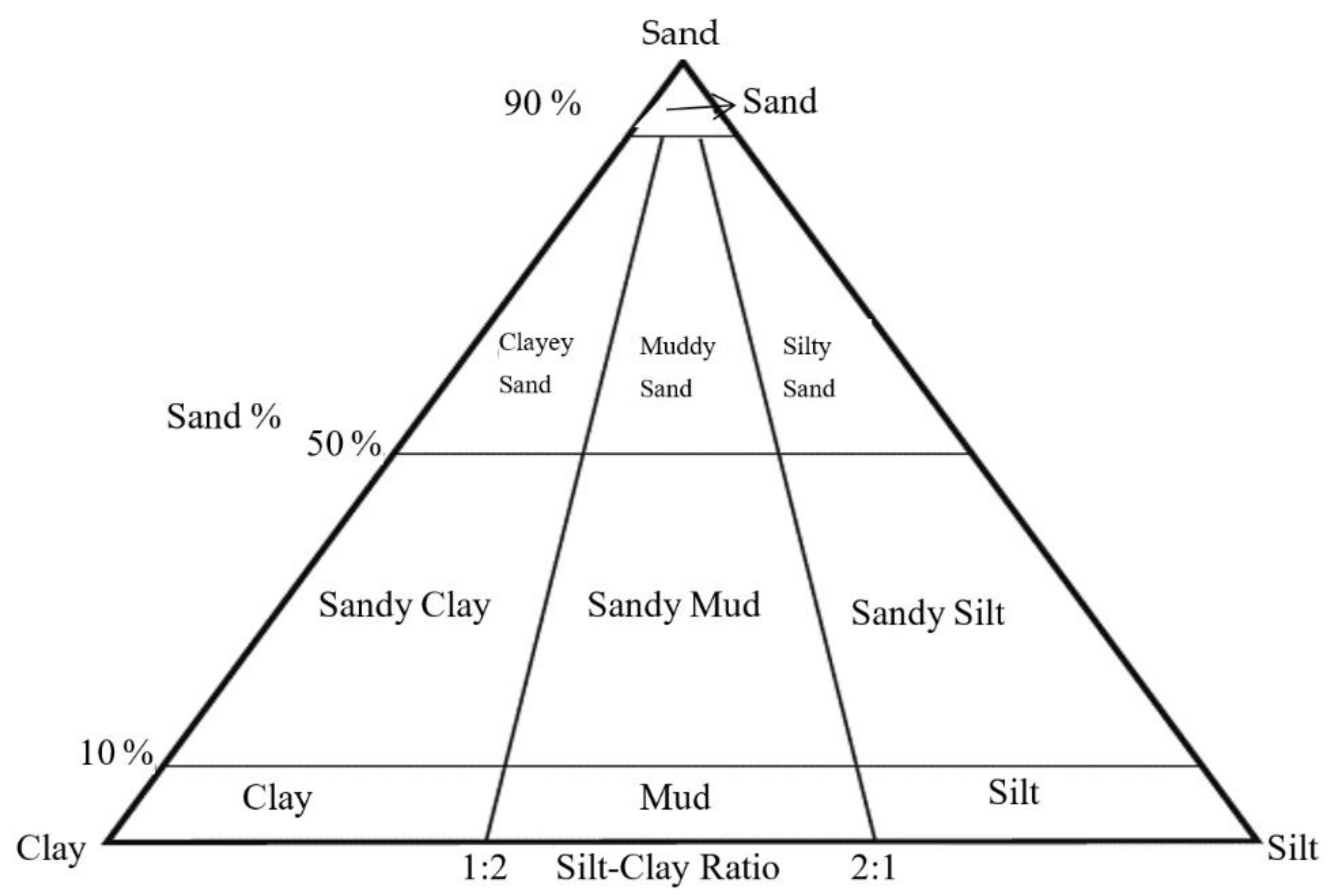
The average relaxation times of various sediments are shown in

Table 2. Average relaxation time for different sediment types.

Sediment Type	Relaxation Time (μs)
Medium sand	0.15
Fine sand	0.17
Coarse silt	0.13
Medium silt	0.06
Fine silt	0.03
Clay	0.02

[17]. By comparing the result τ_relax with the values in Table 2, we can classify the sediment categories. However, it should be noted that the naming methods of the sediment types in Table 2 are different from the commonly used naming method. The nomenclature method in Table 2 is derived from the Udden–Wentworth equal-scale granulation classification standard, where the sediment can be divided into four categories of clay, silt, sand, and gravel; altogether, there are 15 subcategories according to the particle size [30]. Commonly used sediment categories are named according to the relative proportion of different particle size components [31] (Figure 3 shows the Folk naming result). As the proportion of sediment compositions is difficult to be calculated using the classification methods based on either spectral ratio or instantaneous attributes, only results such as those in Table 2 can be obtained. Therefore, according to the Fokker method and the Udden–Wentworth ratio grading classification standard, the sediment category is simplified into sand, silt, and clay. In addition, considering that mud is also a common category in actual measurement, it also needs to be added as a category. According to the results of the Fokker method, mud is a mixture of clay and silt, and its relaxation time should be between that of clay and silt, varying from 0.02 μs to 0.03 μs.

Since the range of the silt category relaxation time is large, while the relaxation times of other categories are small, we can adjust the relaxation time ranges during the simplification of categories to prevent other sediments from being mistakenly classified into silt. The adjusted relaxation time ranges are shown in

Table 3. Relaxation time range for different sediment types after adjustment.

Sediment Type	Relaxation Time Range (μs)
Sand	τrelax ≥ 0.095
Silt	0.045 ≤ τrelax < 0.095
Mud	0.020 < τrelax < 0.045
Clay	τrelax ≤ 0.02

, where 0.095 is calculated through (0.13 + 0.06)/2 and 0.045 is calculated through (0.03 + 0.06)/2.

3. Experiment and Results

To verify the effectiveness of the proposed method, real data experiments were performed. Experimental areas were located in Caofeidian Port area of Tangshan Port in China. The water depth was 5–11 m. Edgetech 3200X-STAR SBP was used for this measurement. The Chirp wave frequency range was set to 0.5–8.0 KHz, and the sampling interval was 0.08 ms. The transmitting power was 2000 W; the speed was about 4–5 knots. The borehole sampling and geotechnical analysis results showed that the sediment in this area is mainly composed of mud, silt, silty clay, and silty sand.

3.1. Case 1

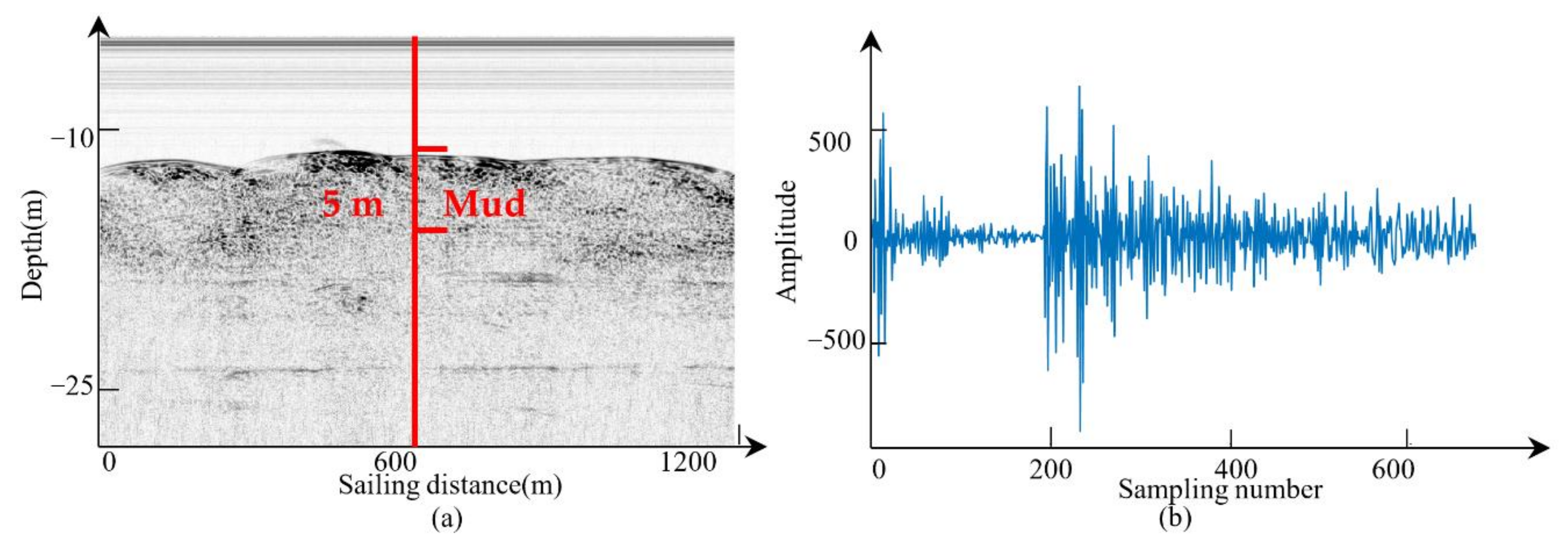
Firstly, the Hilbert transform method was applied to obtain the instantaneous amplitude data. Then, according to the amplitude distribution histogram, the amplitude data were converted into 0–255 to form an SBP image [2], as shown in Figure 4a. From the SBP image, we could locate the positions of the layer reflections. In this case, mud was the first layer, and the borehole sampling did not show the sediment types of deeper layers. The mud layer was located below the 200th sampling point. We also found that, except for the strong reflections, there are some scattering waves in the SBP image, which may have made the classification less robust.

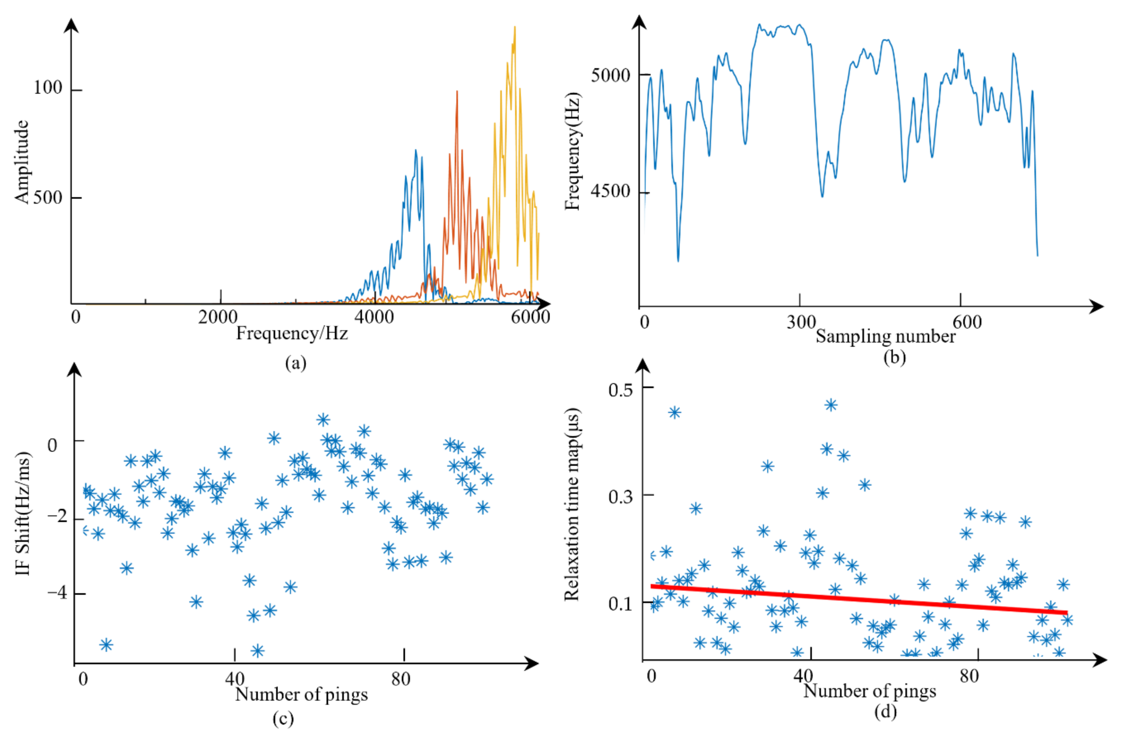
MVMD was first applied to data of one ping. After calculating the mean and standard of each mode, the distribution characteristic of modes in the frequency domain was analyzed, and the spectral overlap between two modes was assessed. The final number of modes in one ping was determined as three. Figure 5a shows the situation of the spectral overlap of decomposed modes. It can be noted that, through the proposed MVMD method, the mode u_k was mostly compact around a center angular frequency ω_k, and different modes were away from each other in the frequency domain. Figure 5b–d show the results of different modes.

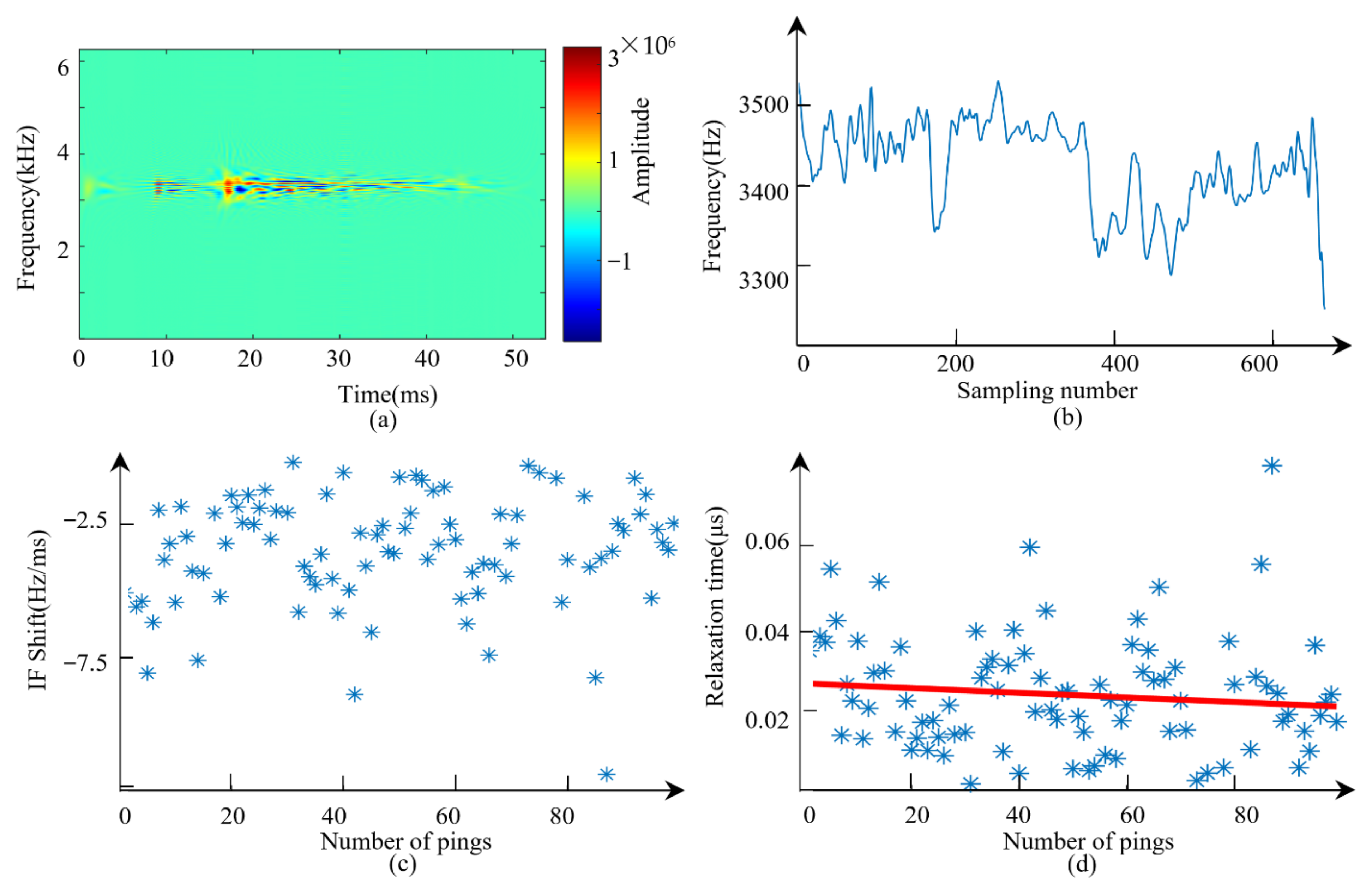
WVD shows the time–frequency distribution of the input signal. At every sampling time, a set of frequencies can be obtained. Thus, WVD has high time and frequency resolution. The WVD of one mode is shown in Figure 6a.

To obtain the IF series of one mode, the first moment of its corresponding WVD along the y-axis was calculated. Combining IF series derived from different WVD maps of different modes, a final IF series could be obtained, as shown in Figure 6b.

The IF curve obtained using the proposed method was smooth although small fluctuation could still be observed in Figure 6b. The fluctuation of the IF series may have been caused by the scatters and the existence of small reflectors. The line fitting was applied to the IF series in the selected range (200th–300th sampling point in this case). The slope of the fitted line was f_shift. After calculating the f_shift of 101 pings of the data around the location of the drill hole, a plot could be obtained (Figure 6c). The relaxation times were obtained using Equation (12). Some relaxation times with negative values were removed. The final relaxation time map is shown in Figure 6d. We extracted an IF series corresponding to the negative relaxation time and found that the inaccurate locations of reflectors could have led to these negative values. After eliminating these outliers, we then applied the robust estimate to the relaxation time map. Some anomalies could be suppressed after robust estimation, and a robust result could be achieved.

Geotechnical analysis was applied to the drill hole sample. The analysis result shows that the sediment here was mud and was behaving plastically. A large amount of debris and a small amount of silt mass were also observed in this drill hole sample. The relaxation time here was between 0.021 μs and 0.026 μs. Compared with the results in Table 3, we can conclude that the sediment type was mostly mud, consistent with the geotechnical analysis result.

3.2. Case 2

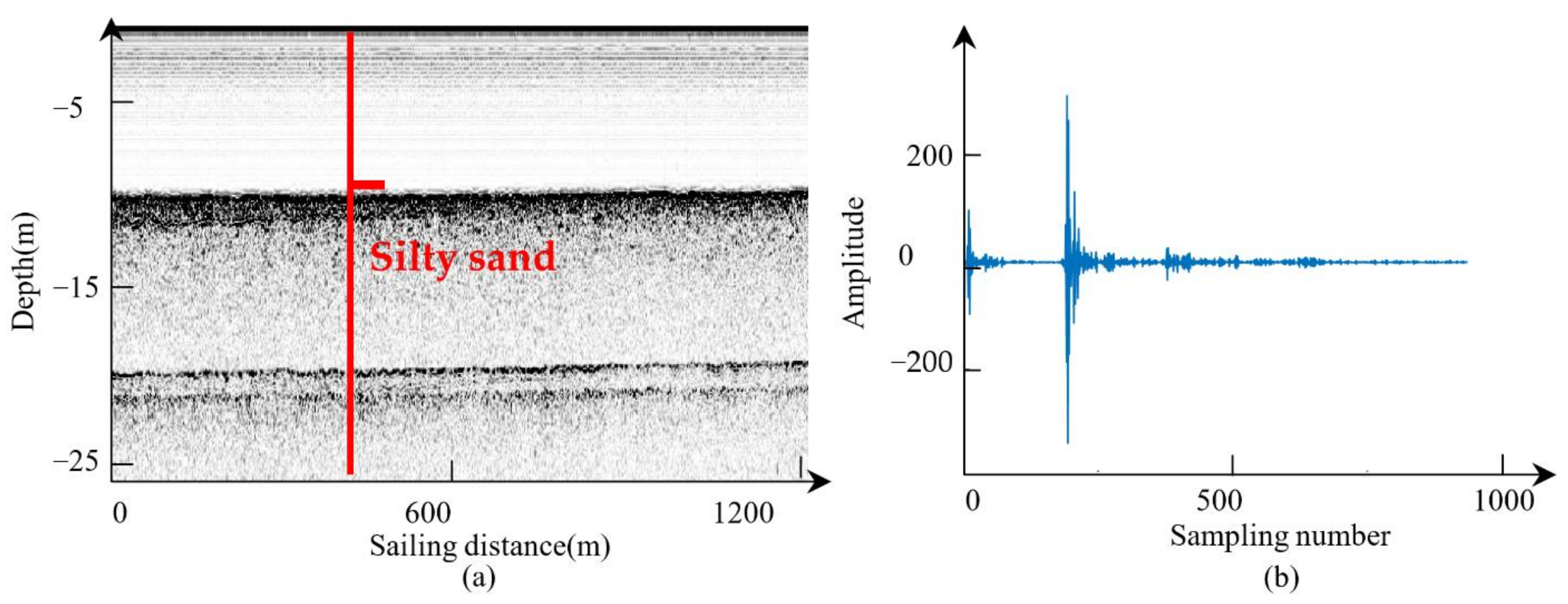
The original data were transformed into a grayscale image, as shown in Figure 7a. Figure 7b shows the data of one ping. From the SBP image, we found that there were many scattering waves below the seafloor. Because of the high attenuation of the acoustic energy in this area, the emitted acoustic wave could not reach deep reflectors. Some reflections with the depth of 20 m were similar to the seafloor, which were multiples caused by the secondary reflections from the sea surface to the seafloor. MVMD was applied first, and the original data were decomposed into several separate modes. The spectral overlap of these modes is shown in Figure 8a. WVD was then applied. By applying the first moment calculation to the WVD along the y-axis, the IF series could be obtained. The final IF series was achieved by combining the IF series of every mode, as shown in Figure 8b. After calculating the relaxation times of 101 pings of the data around the location of the drill hole, a relaxation time map was obtained, as shown in Figure 8d. We then applied the robust estimate to the relaxation time map and the relaxation time was around 0.10 μs. The estimated relaxation time fluctuated greatly, which could have been caused by the non-determinacy introduced by the scattering waves.

The geotechnical analysis of the drill hole sample shows that the sediment here was silty sand. The relaxation time estimated here was close to the relaxation time of middle sand and coarse silt in Table 2. Referring to the relaxation time results after our category simplification in Table 3, the sediment was defined as sand. Thus, the sediment type determined using the proposed method was consistent with that provided by the drill hole. Accordingly, the effectiveness of the proposed method was verified.

3.3. Case 3

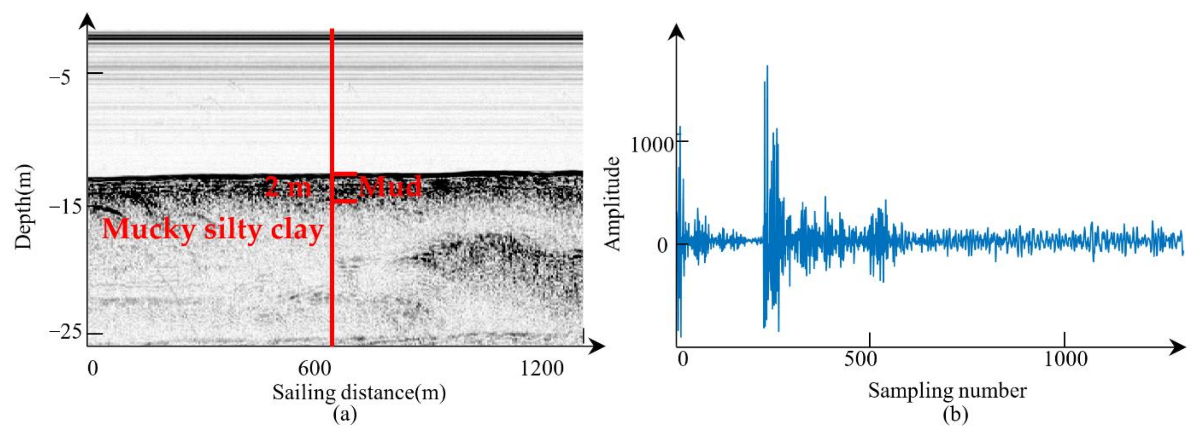
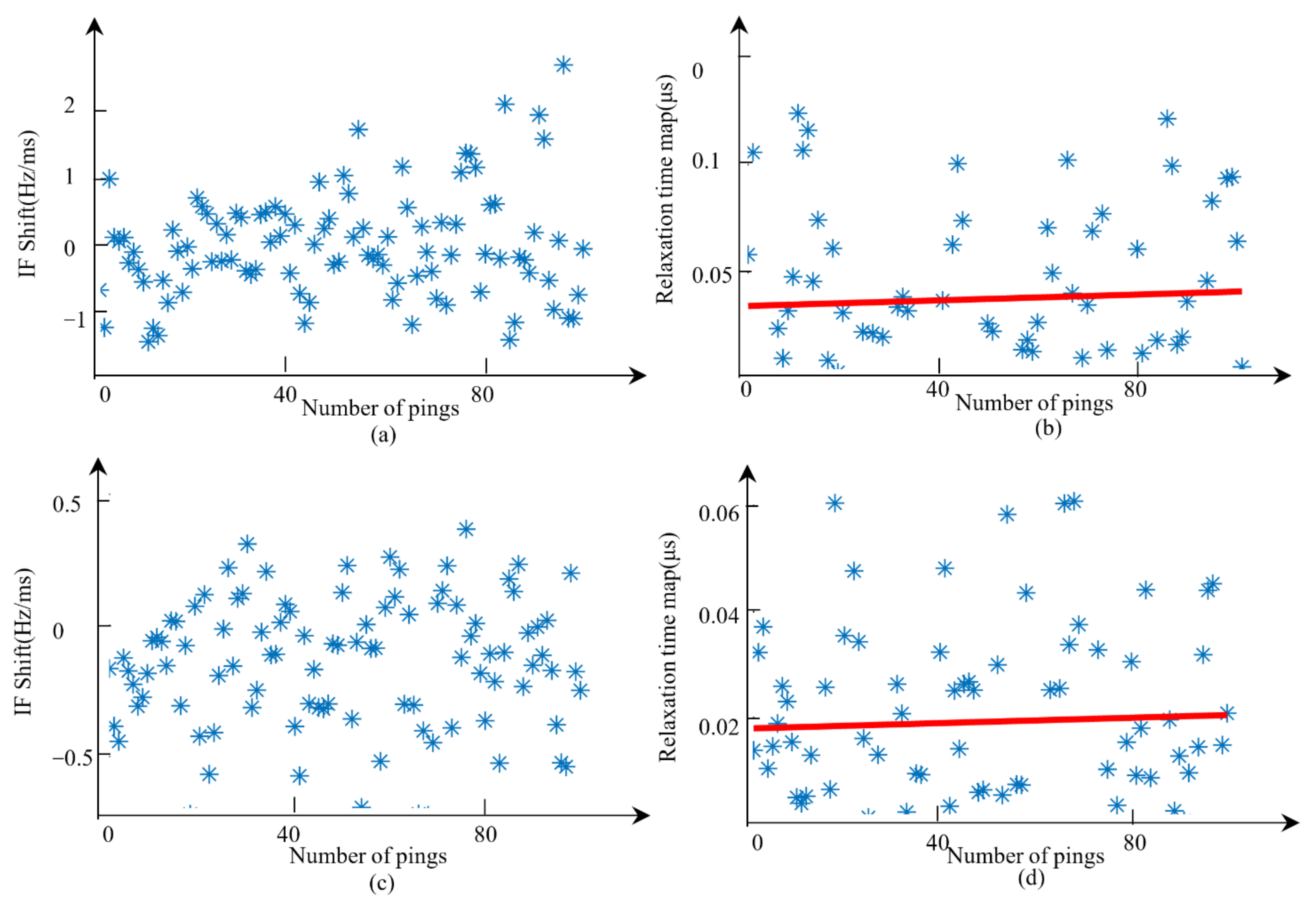
The original data were transformed into a grayscale image, as shown in Figure 9a. From the SBP image, we found two layers. The first layer was located between the 230th and 260th sampling points. The second layer was located below the 260th sampling point. It was also observed in the SBP image that there were many scattering waves below the seafloor. The scattering waves and the thin thickness of the first layer increased the difficulty in estimating the relaxation time, as scattering waves may introduce outliers, while thin thickness means that fewer observations can be used in relaxation time estimation. MVMD was applied first. Figure 10a shows that the number of modes was determined as four, and the original data were decomposed into four separate modes. The WVD of each mode was calculated after MVMD. Then, by applying the first moment calculation to the WVD along y-axis, the IF series of each mode could be obtained. The final IF was achieved by combining the IF series of every mode, as shown in Figure 10b. After calculating the relaxation times of 101 pings of the data around the location of the drill hole, a relaxation time map was achieved. We then applied the robust estimate to the relaxation time map, as shown in Figure 11b,d.

From the relaxation time map in Figure 11, we found that the relaxation time of the first layer was between 0.032 μs and 0.040 μs, and the relaxation time of the second layer was between 0.018 μs and 0.020 μs. The sediment type of the first layer was mud, and the sediment type of the second layer was clay. The geotechnical analysis of the drill hole sample showed that the sediment here was mud and mucky silty clay. Thus, the sediment type determined by the proposed method was basically consistent with that provided by the drill hole. However, it is worth noting that, from the relaxation time maps, the distribution ranges of relaxation time discrete points under silt and silty clay are relatively close. Therefore, although the distinction between the two types of sediments was achieved, the difference between these two sediments in terms of relaxation time is small.

4. Discussions

4.1. The Effectiveness of MVMD

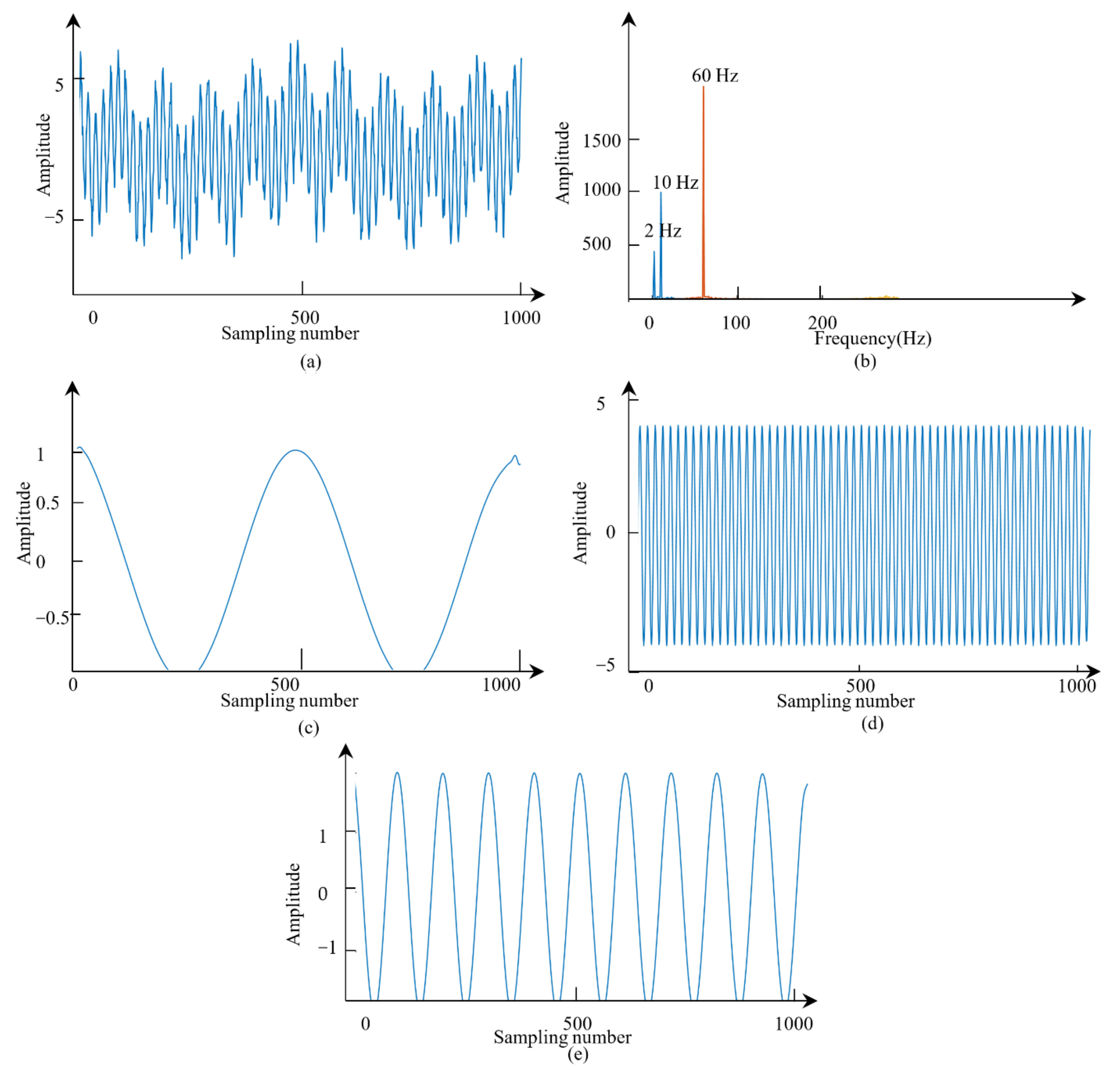
To verify the ability and effectiveness of the proposed method in the determination of the number of modes K and the decomposition of signals, a simulated signal was generated, as shown in Figure 12a. The simulated signal y can be expressed as

$$y=\cos (4\pi t)+2\cos (20\pi t)+4\cos (120\pi t)+n,$$

(34)

where n is the noise. This signal was composed of three cosine signals (with frequency 2 Hz, 10 Hz, and 60 Hz, respectively). Using the proposed MVMD method, K was first determined as 3. VMD was then applied to the simulated signal, and the modes after decomposition were as shown in Figure 12c–e. In this case, the spectral ratio is shown in Figure 12b. It is very clear that the three modes had center frequencies of 2 Hz, 10 Hz, and 60 Hz, respectively, and the decomposed signals were very close to the original sub-signals.

4.2. Robust Line Fitting

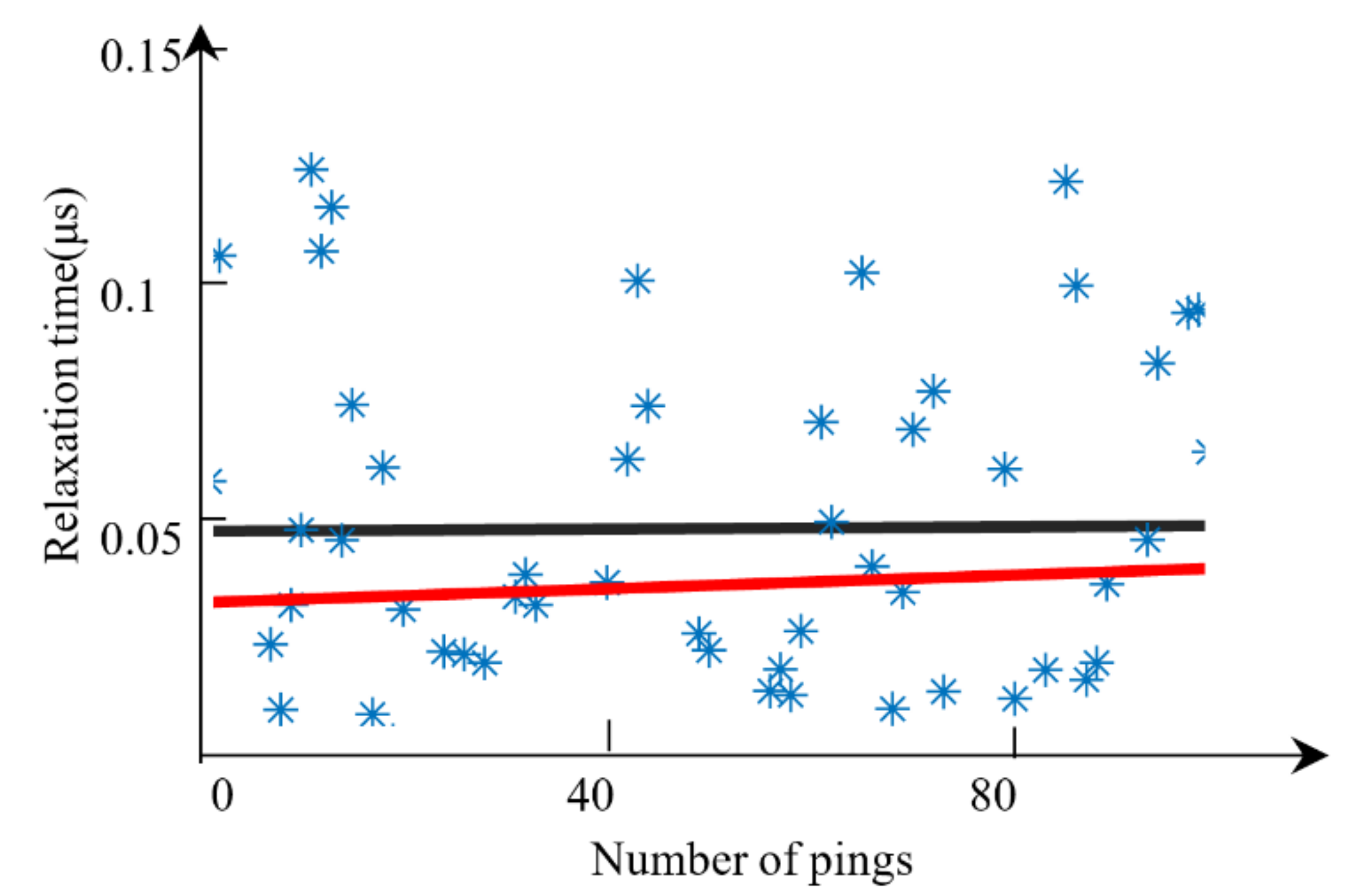
After calculating a set of relaxation times for 101 pings, a line fitting based on the robust estimation theory was applied to the relaxation time map. Here, we compared the difference between line fitting results with or without robust estimation. The relaxation time map is shown in Figure 13, and the black line shows the line fitting using the least-squares method, while the red line shows the line fitting using the robust line fitting algorithm. This sediment type was mud, with a relaxation time between 0.020 μs and 0.045 μs. The estimated relaxation time using the black line was relatively high (between 0.048 μs and 0.049 μs), which may have been caused by the outliers with high relaxation times, while the used robust method obtained a more credible result (between 0.032 μs and 0.040 μs).

4.3. Comparison with Traditional Methods

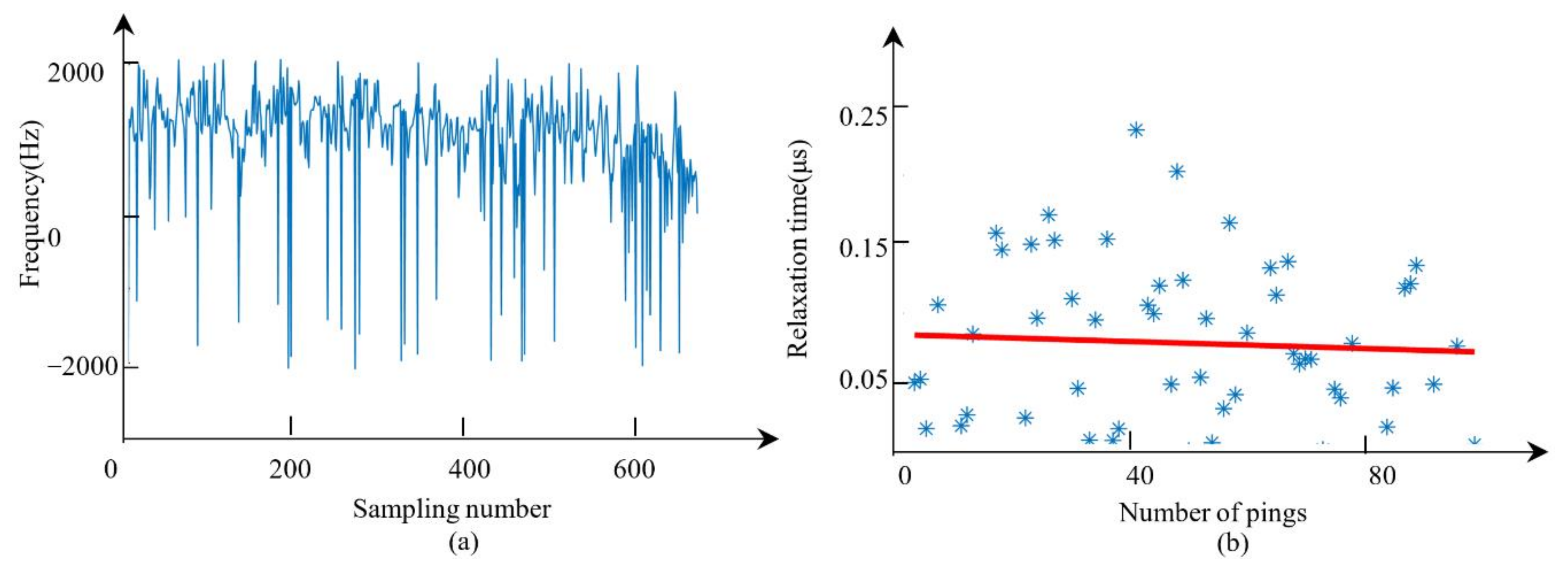
The typically used IF calculation method is based on Equation (24). The calculated IF series of one ping is shown in Figure 14a based on the real data in case 1. There were several outliers in the IF series. Although the robust line fitting of the relaxation time map showed that the relaxation time was near 0.08 μs, which is close to the relaxation time of mud. As shown in Figure 14b, too many outliers were removed before generating the relaxation time map, which led to the few points in the fitting. Thus, the result was not reliable.

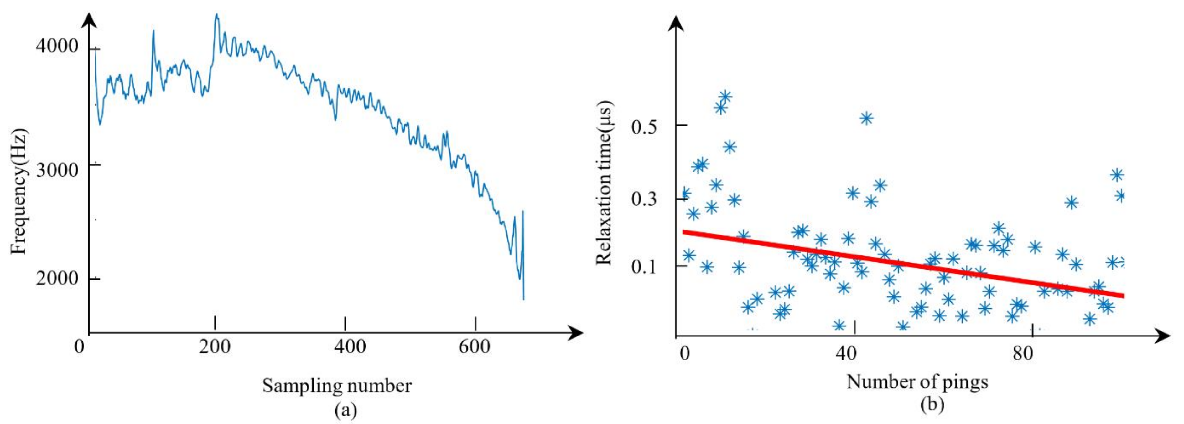
In the work of Robb et al. [18], they tested the performance of WVD using a set of real experiments and concluded that WVD is suitable for the relaxation time estimation of correlated Chirp SBP signals. Here, we also directly applied the WVD to the real data in case 1. The obtained IF series is shown in Figure 15a, and the relaxation time map and the fitted line are shown in Figure 15b. The estimated relaxation time was about 0.1 μs, while the relaxation time in this sediment type (mud) is about 0.02–0.03 μs. Thus, the estimated result was far away from the ground truth. This situation may have been caused by cross-terms. Cross-terms are generated by the WVD when the input signal is multi-component and can lead to inaccurate IF values.

5. Conclusions

In this paper, we presented the MVMD-WVD method for reliable IF calculation and used the relaxation time model to obtain relaxation time maps. To suppress the influence of outliers, a robust least-squares algorithm was employed to estimate robust relaxation times from the relaxation time map. Final sediment classification could be achieved through the relaxation time look-up table. In conclusion, the sediment classification method presented in this paper provides a new reliable way to explore the relationship between the latent sediment characteristics and the IF series. Furthermore, our experiments show that the proposed method is an effective way of classifying sub-bottom sediments.

However, further improvements in IF calculation can still be achieved, since VMD is not specifically designed for sonar signal processing. Moreover, the proposed method is still away from practical application in complex sediment environments, and further research may be needed for a finer classification of the sub-bottom. In future work, we will combine more prior characteristics in SBP sonar signals with MVMD to effectively obtain a more reliable IF series.

References

1. Lurton, X. An Introduction to Underwater Acoustic: Principles and Applications, 2nd ed.; Springer: Chichester, UK, 2010; pp. 372–379. [Google Scholar]
2. Li, S.; Zhao, J.; Zhang, H.; Bi, Z.; Qu, S. A Novel Horizon Picking Method on Sub-Bottom Profiler Sonar Images. Remote Sens. 2020, 12, 3322. [Google Scholar] [CrossRef]
3. Zhao, J.; Li, S.; Zhang, H.; Feng, J. Comprehensive Sediment Horizon Picking From Subbottom Profile Data. IEEE J. Ocean. Eng. 2018, 44, 524–534. [Google Scholar] [CrossRef]
4. Idczak, J.; Brodecka-Goluch, A.; Łukawska-Matuszewska, K.; Graca, B.; Gorska, N.; Klusek, Z.; Pezacki, P.D.; Bolałek, J. A geophysical, geochemical and microbiological study of a newly discovered pockmark with active gas seepage and submarine groundwater discharge (MET1-BH, central Gulf of Gdańsk, southern Baltic Sea). Sci. Total Environ. 2020, 742, 140306. [Google Scholar] [CrossRef]
5. Fakiris, E.; Blondel, P.; Papatheodorou, G.; Christodoulou, D.; Dimas, X.; Georgiou, N.; Kordella, S.; Dimitriadis, C.; Rzhanov, Y.; Geraga, M.; et al. Multi-Frequency, Multi-Sonar Mapping of Shallow Habitats—Efficacy and Management Implications in the National Marine Park of Zakynthos, Greece. Remote Sens. 2019, 11, 461. [Google Scholar] [CrossRef] [Green Version]
6. Hoffmann, J.J.L.; Von Deimling, J.S.; Schröder, J.F.; Schmidt, M.; Held, P.; Crutchley, G.J.; Scholten, J.; Gorman, A.R. Complex Eyed Pockmarks and Submarine Groundwater Discharge Revealed by Acoustic Data and Sediment Cores in Eckernförde Bay, SW Baltic Sea. Geochem. Geophys. Geosyst. 2020, 21, e2019GC008825. [Google Scholar] [CrossRef]
7. Garcia-Gil, S.; Vilas, F.; Garcia-Garcia, A. Shallow gas features in incised-valley fills (Ría de Vigo, NW Spain): A case study. Cont. Shelf Res. 2002, 22, 2303–2315. [Google Scholar] [CrossRef]
8. Kato, Y.; Fujinaga, K.; Nakamura, K.; Takaya, Y.; Kitamura, K.; Ohta, J.; Toda, R.; Nakashima, T.; Iwamori, H. Deep-sea mud in the Pacific Ocean as a potential resource for rare-earth elements. Nat. Geosci. 2011, 4, 535–539. [Google Scholar] [CrossRef]
9. Stevenson, I.; McCann, C.; Runciman, P. An attenuation-based sediment classification technique using Chirp sub-bottom profiler data and laboratory acoustic analysis. Mar. Geophys. Res. 2002, 23, 277–298. [Google Scholar] [CrossRef]
10. Vardy, M.; Vanneste, M.; Henstock, T.; Clare, M.A.; Forsberg, C.F.; Provenzano, G. State-of-the-art remote characterization of shallow marine sediments: The road to a fully integrated solution. Near Surf. Geophys. 2017, 15, 387–402. [Google Scholar] [CrossRef]
11. Mohamed, S. Seabed Classification Using Sub-Bottom Profiler. Master’s Thesis, Delft University of Technology, Delft, The Netherlands, 2011. [Google Scholar]
12. Plets, R.M.K. The Acoustic Imaging, Reconstruction and Characterization of Buried Archaeological Material. Ph.D. Thesis, University of Southampton, Southampton, UK, 2007. [Google Scholar]
13. Plets, R.; Dix, J.; Adams, J.; Best, A. 3D reconstruction of a shallow archaeological site from high-resolution acoustic imagery: The Grace Dieu. Appl. Acoust. 2008, 69, 399–411. [Google Scholar] [CrossRef] [Green Version]
14. Jannsen, D.; Voss, J.; Theilen, F. Comparison of methods to determine q in shallow marine sediments from vertical reflection seismograms. Geophys. Prospect. 1985, 33, 479–497. [Google Scholar] [CrossRef]
15. Pinson, L.J.W.; Henstock, T.; Dix, J.K.; Bull, J. Estimating quality factor and mean grain size of sediments from high-resolution marine seismic data. Geophysics 2008, 73, G19–G28. [Google Scholar] [CrossRef] [Green Version]
16. Schock, S.G. The Chirp—High Resolution, Quantitative Subbottom Profiler. Ph.D. Thesis, University of Rhode IsIand, Kingston, RI, USA, 1989. [Google Scholar]
17. Panda, S. Remote Acoustic Evaluation of Seafloor Sediment Properties. Ph.D. Thesis, University of Rhode IsIand, Kingston, RI, USA, 1992. [Google Scholar]
18. Robb, G.B.N.; White, P.R.; Bull, J.M.; Best, A.I.; Leighton, T.G.; Dix, J.K. The Estimation of Geo-Acoustic Properties from Broadband Acoustic Data, Focusing on Instantaneous Frequency Techniques. Inst. Sound Vib. Res. Southampt. UK Tech. Rep. 2002, 298, 40. [Google Scholar]
19. Cohen, L. Time frequency distributions—A review. Proc. IEEE 1989, 77, 941–981. [Google Scholar] [CrossRef] [Green Version]
20. Chen, V.C.; Qian, S. Joint time-frequency transform for radar range doppler imaging. IEEE Trans. Aerosp. Electron. Syst. 1998, 34, 486–499. [Google Scholar] [CrossRef]
21. Andria, G.; Savino, M. Interpolated smoothed pseudo Wigner-Ville distribution for accurate spectrum analysis. IEEE Trans. Instrum. Meas. 1996, 45, 818–823. [Google Scholar] [CrossRef]
22. Yegireddi, S.; Thomas, N. Segmentation and classification of shallow subbottom acoustic data, using image processing and neural networks. Mar. Geophys. Res. 2014, 35, 149–156. [Google Scholar] [CrossRef]
23. Lee, G.H.; Kim, H.J.; Kim, D.C.; Yi, B.Y.; Nam, S.M.; Khim, B.K.; Lim, M.S. The acoustic diversity of the seabed based on the similarity index computed from Chirp seismic data. ICES J. Mar. Sci. 2008, 66, 227–236. [Google Scholar] [CrossRef] [Green Version]
24. Dragomiretskiy, K.; Zosso, D. Variational Mode Decomposition. IEEE Trans. Signal Process. 2013, 62, 531–544. [Google Scholar] [CrossRef]
25. Xue, Y.-J.; Cao, J.-X.; Wang, X.-J.; Du, H.-K. Estimation of seismic quality factor in the time-frequency domain using variational mode decomposition. Geophysics 2020, 85, V329–V343. [Google Scholar] [CrossRef]
26. Taner, M.T.; Koehler, F.; Sheriff, R.E. Complex seismic trace analysis. Geophysics 1979, 44, 1041–1063. [Google Scholar] [CrossRef]
27. Barnes, A.E. Theory of 2-D complex seismic trace analysis. Geophysics 1996, 61, 264–272. [Google Scholar] [CrossRef]
28. Qiu, W.N. The Theory and Method of Surveying Data Processing, 2nd ed.; WuHan University Press: Wuhan, China, 2008; pp. 126–140. [Google Scholar]
29. Li, S.; Zhao, J.; Zhang, H.; Zhang, Y. Automatic Detection of Pipelines from Sub-bottom Profiler Sonar Images. IEEE J. Ocean. Eng. 2021, in press. [Google Scholar] [CrossRef]
30. Zhao, D.B. Discussion on Common Classification and Nomenclature Methods of Sediment Grain Size. Mar. Geol. Lett. 2009, 25, 41–44. [Google Scholar]
31. Folk, R.L. Practical Petrographic Classification of Limestones. AAPG Bull. 1959, 43, 1–38. [Google Scholar] [CrossRef]
Figure 1. Flowchart of the proposed method.
Remotesensing 13 04809 g001
Figure 2. Illustration of the spectral overlap and the relaxation time map. (a) The spectral overlap. (b) The relaxation time map and its line fitting.
Remotesensing 13 04809 g002
Figure 3. Illustration of the sediment nomenclature.
Remotesensing 13 04809 g003
Figure 4. The measurement data. (a) The SBP image. (b) The raw data of one ping.
Remotesensing 13 04809 g004
Figure 5. Illustration of the MVMD result. (a) The spectral ratio of the decomposed modes of one ping. (b) The first mode after decomposition. (c) The second mode after decomposition. (d) The third mode after decomposition.
Remotesensing 13 04809 g005
Figure 6. Illustration of WVD, IF series, and the relaxation time map. (a) The WVD result of one mode. (b) The IF series data of one ping. (c) The IF shift data of 101 pings. (d) The relaxation time map and the robust line fitting based on relaxation time map.
Remotesensing 13 04809 g006
Figure 7. The measurement data. (a) The SBP image. (b) The raw data of one ping.
Remotesensing 13 04809 g007
Figure 8. Illustration of VMD, IF series, and the relaxation time map. (a) The spectral overlap situation after VMD. (b) The IF series data of one ping. (c) The IF shift data of 101 pings. (d) The robust line fitting based on a relaxation time map.
Remotesensing 13 04809 g008
Figure 9. The measurement data. (a) The SBP image. (b) The raw data of one ping.
Remotesensing 13 04809 g009
Figure 10. Illustration of VMD and the IF series. (a) The spectral overlap situation after VMD. (b) The IF series data of one ping.
Remotesensing 13 04809 g010
Figure 11. Illustration of the IF series and the relaxation time map. (a) The IF shift data of 101 pings of the first layer. (b) The robust line fitting based on a relaxation time map of the first layer. (c) The IF shift data of 101 pings of the second layer. (d) The robust line fitting based on a relaxation time map of the second layer.
Remotesensing 13 04809 g011
Figure 12. Illustration of the MVMD. (a) The original data. (b) The spectral ratio of the decomposed modes. (c) The first mode. (d) The second mode. (e) The third mode.
Remotesensing 13 04809 g012
Figure 13. Illustration of the robust line fitting. The black line is the classical line fitting, while the red line is the robust line fitting.
Remotesensing 13 04809 g013
Figure 14. Illustration of the IF series using traditional method and the relaxation time map. (a) The IF series. (b) The robust line fitting based on the relaxation time map.
Remotesensing 13 04809 g014
Figure 15. Illustration of the IF series using WVD and the relaxation time map. (a) The IF series. (b) The robust line fitting based on the relaxation time map.
Remotesensing 13 04809 g015