Measurement of Seafloor Acoustic Backscatter Angular Dependence at 150 kHz Using a Multibeam Echosounder

Abstract

Acoustic seafloor measurements with multibeam echosounders (MBESs) are currently often used for submarine habitat mapping, but the MBESs are usually not acoustically calibrated for backscattering strength (BBS) and cannot be used to infer absolute seafloor angular dependence. We present a study outlining the calibration and showing absolute backscattering strength values measured at a frequency of 150 kHz at around 10–20 m water depth. After recording bathymetry, the co-registered backscattering strength was corrected for true incidence and footprint reverberation area on a rough and tilted seafloor. Finally, absolute backscattering strength angular response curves (ARCs) for several seafloor types were constructed after applying sonar backscattering strength calibration and specific water column absorption for 150 kHz correction. Thus, we inferred specific 150 kHz angular backscattering responses that can discriminate among very fine sand, sandy gravel, and gravelly sand, as well as between bare boulders and boulders partially overgrown by red algae, which was validated by video ground-truthing. In addition, we provide backscatter mosaics using our algorithm (BBS-Coder) to correct the angle varying gain (AVG). The results of the work are compared and discussed with the published results of BBS measurements in the 100–400 kHz frequency range. The presented results are valuable in extending the very sparse angular response curves gathered so far and could contribute to a better understanding of the dependence of backscattering on the type of bottom habitat and improve their acoustic classification.

1. Introduction

Ocean shelves and shallow waters are exposed to increasing anthropogenic pressure and economic exploitation. Marine areas offer potential for raw material exploitation and offshore energy production sites that require infrastructure such as pipelines and cables on the seabed. Shallow areas are also intensively exploited by fishing using bottom trawls. Human activities such as intensive fishing and polluting the oceans with sewage may have a destructive effect on the benthic flora and fauna and cause secondary harm through, e.g., reef and habitat destruction. Mapping and monitoring the individual habitats and identifying potential harm or even destruction imply a need for reliable remote sensing of the seafloor. Satellites have become commonly used devices for mapping land areas, whereas, for investigating the marine environment, acoustic measurements are more suitable because, among other reasons, they are not limited by the depth of the euphotic layer. Hydroacoustic swath devices are very efficient tools for underwater spatial remote sensing, enabling large-scale high-resolution mapping and detection of objects in the water column and on the seafloor, thus supporting environmental monitoring of benthic areas. There are well-established methodologies for acoustic-based mapping with confirmed reliability (e.g., [1,2,3]). High-frequency MBES recordings have been suggested and proven to be a valuable tool for this type of research [4,5,6]. In recent years (2017–2020), the ECOMAP project has been exploring the use of swath devices and shallow marine seismic and LIDAR measurements to study the seabed environment (e.g., [7,8,9]).

The main task of industrial MBES measurements is bathymetry, but systems have improved with regard to backscattering strength measurements of both the water column and the seafloor [10]. Especially in shallow water less than 20 m in water depth, ship-based MBES offers great potential for recording sidescan-like snippets [11]. The intensity of backscattered signals depends on many parameters, such as the geoacoustic properties of the seabed, but it is also controlled by the sonar-target geometry, including the individual beam incidence angles and varying bottom reverberation areas (Figure 1) modulated by the local slope of the seabed.

The slope of the seabed has an effect on the BBS [12], due not only to modifications of the reflection angle but also to differences in footprint area. A flat bottom assumption can cause misinterpretation of acoustic signals in the description and classification of bottom habitats, especially when an offset of a few degrees appears unnoted [7]. The impact of slope on signals recorded by multibeam echosounders is even more pronounced in very shallow environments and those with significant topographic variations (Figure 1b).

We can divide parameters that influence registered echo signal into three groups: (i) device-based parameters (e.g., frequency, transducer sensitivity, directivity patterns), (ii) environmental parameters, i.e., acoustic absorption of water during two-way travel (e.g., salinity, temperature), and (iii) seafloor parameters modulating backscattering strength, i.e., physical interaction processes between signal and scattering objects (e.g., roughness of seabed, sediment porosity). To use both absolute backscattering strength and incident-specific echo shape bottom characteristics (ARC), we must know how the parameters in the first two groups modulate the acoustic signals.

MBES measurement with corrected backscattering strength is generally sparse, although affordable [13]. Some companies (e.g., Kongsberg, NORBIT) provide calibration files based on tank measurements and, thus, offer the ability to record absolute backscattering strength values on the fly. In this work, we also outline how we performed the calibration, which was one goal of the EU-funded project BONUS ECOMAP, where we used a calibrated NORBIT STX prototype sonar.

Acoustic measurements of the seafloor with various incidence and corrected backscattering strength are extremely rare [13,14,15,16,17,18]. In this study, we intended to deliver a set of specific records of this kind, the first ones gathered in the Baltic Sea so far. In addition, we discuss how such measurements can improve acoustic seafloor classification and compare absolute backscattering strength and ARCs to the few reports published so far.

The recorded echoes of acoustic signals scattered on the seabed (backscatter) together with bathymetry are often used to classify benthic habitats [8,19,20,21]. The backscatter parameter is not the real BBS value, but the relative signal intensity recorded by the receiver, which is modified so that the relative intensity values correspond to one angle of incidence of the acoustic beam on the bottom. A popular and commercially used tool for preparing such backscatter mosaics is Geocoder, presented by Fonseca and Calder [22]. Geocoder uses the data recorded by MBESs, performs radiometric and geometric correction, and interpolates the intensity values into the final backscatter mosaic.

1.1. Models, Classification, and Calibration

The purpose of using corrected backscattering intensity is to provide an absolute value of the bottom backscattering strength of the seafloor. This requires the use of sonar, whose response on the seafloor is accurately known with regard to the sensitivity during transmission and reception of the signal and taking into account the frequency and angle of incidence. Moreover, this requires applying accurate compensations for transmission losses related to medium and beam geometry and footprint extent to recorded BBS values [16,23].

In most applications for MBES data collection and processing, it is possible to apply environmental parameters measured by, e.g., CTD. This procedure adjusts backscatter data to compensate refraction and attenuation of acoustic signals while traveling in the water. For the calculations presented in this paper, we used an absorption coefficient, which is the result of absorption calculations from a formula given by Francois and Garrison using averaged environmental parameters [24]. The last step to correct intensity signals for propagation and attenuation losses is to refer their value to the beam footprint area on the bottom. Most of the time, a flat bottom assumption is used to calculate this value [23,25].

A compendium of good practices for backscatter collection and processing prepared by the BSWG GeoHab group is the first document of its kind focusing on the quality of MBES acoustic intensity data [23]. Whereas IHO hydrographic standards [26] adequately described MBES bathymetry measurements, standards related to MBES backscatter measurements are rarely standardized in the literature. Ideally, backscatter should be based on full calibration of the sonar sensitivity in transmission and reception, giving access to absolute backscatter strength levels [16,23].

The methods of benthic habitat classification can be divided into two groups: empirical approaches [27] and approaches based on physical modeling of the seabed with various geoacoustic parameters [28]. In the case of MBES, the empirical approach uses the registered backscattered intensity from areas with ground-truth samples and, optionally, bathymetry to assign segmented seabed data to habitat types, creating classified polygons [8,19,20,21]. The physical model-based approach predicts backscattering strength by modeling the acoustic propagation given the respective geoacoustic properties of the seabed, compares measured values with modeled values, and, on this basis, differentiates classes. This approach depends on the model used to describe backscattering from the seabed and the quality of MBES data. The popular APL model was developed for frequencies from 10 to 100 kHz [29]. Backscattering models are not well recognized for frequencies above 100 kHz [15,30]. Modern MBESs for shallow water are usually operated at higher frequencies (typically 150–400 kHz). In the authors’ opinion, difficulties in understanding the phenomenon of backscattering on the seabed are largely due to there being only a small quantity of published calibrated hydroacoustic measurements [15]. A more advanced solution is to prepare a catalog of backscatter parameters for different seabed types at different frequencies and environmental parameters, such as bottom roughness, volume reverberation (including the presence of gas bubbles in the sediment), and grain size, as well as the difference in acoustic impedance between sea water and bottom materials [31]. Measuring the absolute values of angular dependence of the BBS is also necessary to assess the variability of the characteristics of benthic habitats in space and time. Measuring the absolute BBS values may support the development of unsupervised classification methods for previously identified benthic habitats, such as angular range analysis presented by Fonseca et al. [32].

MBES backscatter was the most important parameter for classification of benthic habitats in several works [8,19,20,21]. This highlights the importance of MBES backscatter and the need to measure it as accurately as possible. There is a need to better recognize and investigate the characteristics of backscatter in order to be able to use it for research in the most efficient way [23]. A few studies were conducted recently on calibrating MBESs in reference areas [13,33,34,35]. The most common calibration methods are listed as follows:

• MBES cross-calibration by comparing field data recorded by calibrated SBES, which is based on comparing data recorded in the same place by an acoustically calibrated SBES and an uncalibrated MBES [36]. The SBES transmitter is tilted at different angles to test the angular dependence of the recorded backscatter signal. Correction of MBES recordings is performed on the basis of the measured difference between SBES and MBES measurements. An example is calibration of a Kongsberg EM 2040 MBES using a reference Simrad EK60 in areas located in the Bay of Brest, France [16].
• Calibration with sound sources of known characteristics. This method uses sources with known levels. The aim of the method is to determine receiver and transmitter sensitivities with a defined measurement angle and signal frequency [16,37]. This method has been applied to sonar (Mesotech SM2000/SM20 [38], Kongsberg EM3002 [39], Reson SeaBat T50 [13], Reson SeaBat 7125 [40]). This approach is possible at only a few specialized laboratories worldwide. Foote et al. [41] suggested applying this calibration method to MBES. However, the method contains many difficulties, including the large number of receiving beams, often several hundred.

For the measurements provided in this paper, we utilized the second calibration approach with hydrophones and sound sources of known characteristics. We used a NORBIT iWBMSh (model STX) MBES calibrated in the manufacturer’s laboratory in Trondheim, Norway. In this paper, we present the angular dependencies of absolute values of BBS for specific habitats of the southern Baltic Sea obtained with the acoustically calibrated MBES.

1.2. Goals

Acoustic measurements of the seafloor with various incidence angles and absolute BBS are extremely rare [13,16]. In this study, we provide a set of specific records of this kind, the first ones gathered in the Baltic Sea so far. In addition, we discuss how such measurements can improve acoustic seafloor classification and compare absolute backscattering strength and ARCs to the few cases published so far [13,14,15,16,17]. The main objectives of the work are to develop and discuss (i) the angular dependence of absolute BBS value measurement results for several benthic habitats in the Baltic Sea using transmitted signals of 150 kHz, and (ii) the BBS-Coder applied during the work to achieve an easy-to-interpret backscatter mosaic.

2. Materials and Methods

2.1. Calibration of Multibeam Echosounder

NORBIT’s laboratory tank was used to perform all calibration procedures. They were conducted in order to evaluate the actual detailed MBES characteristics, knowledge of which is necessary to measure physical quantities of the seafloor, such as backscattering strength.

Bottom backscattering strength BBS is defined as

$$BBS=10{\log }_{10}\sigma ,$$

(1)

where σ is the bottom backscattering coefficient [23,30,42]. It denotes the ratio of insonified wave energy backscattered by the seabed with respect to a unit bottom surface.

Bottom backscattering strength is dependent on the frequency of the scattered wave and its angle of incidence to the bottom. It is strongly associated with the physical properties of various types of bottom habitats. BBS depends on many seabed parameters, including density, sound velocity, surface roughness of the seabed surface, and heterogeneity of sediment volume. For most echosounders, the attenuation is so high that the input from volume scattering of the sediment can be described as a function of the reverberation area [23]. Therefore, when considering seafloor backscatter, an interface cross-section is often used, and, when considering the volume scattering, the cross-section for scatterers within the sediment is omitted [43].

With the given measured target strength TS, BBS can be calculated as

$$BBS=TS-BAC,$$

(2)

and the bottom area correction BAC is equal to

$$BAC=10 {\log }_{10}\left(A\right),$$

(3)

where A is the reverberation area insonified by an echosounder.

We can refer to the following classical sonar equation [43]:

$$EL=SL-2TL+TS,$$

(4)

where EL denotes the received echo signal level, SL (source level) is the emitted signal level, TL is the one-way transmission loss describing the signal attenuation due to spreading and absorption in the water column, and TS is target strength describing the backscattering introduced by an investigated object. It should be pointed out that, in an underwater acoustic system, EL is not measured directly, but rather as the level of voltage in the receiving module circuit after energy is transformed from acoustic to electric form. When a set of separate MBES beams is used, instead of EL, we apply the term of beam level BL, which is the received voltage signal level for a particular beam. Moreover, the MBES operation cannot be described by a single value of SL, as it contains specialized signal processing, such as beamforming and matched filtering, each characterized by its own gain, and the directivity properties of particular beams must also be taken into account.

To show all factors that influence TS and BBS measured by the multibeam echosounder, by introducing the device gain DG instead of SL and using the relationship between TS and BBS (Equation (2)), the sonar equation for a given MBES receive beam can be written as

$$BBS=BL-DG+2TL-BAC,$$

(5)

where the device gain DG is the superposition of several factors describing the MBES operation, in both its transmitting and receiving segments, i.e.,

$$DG=OCR+VGA\left(t\right)+PG\left(R{x}_{set}\right)+S{L}_0\left(T{x}_{set}\right)+Di{r}_{Rx}\left(\theta ,\phi \right)+Di{r}_{Tx}\left(\theta ,\phi \right).$$

(6)

OCR is the open circuit response of the receiving array itself, which is defined as the ratio of the RMS voltage produced by the received plane wave to the RMS pressure p of this wave at the transducer face; VGA is the gain of the time-dependent variable gain amplifier applied in the sonar in order to compensate the spherical spreading of the acoustic wave in the water column; PG is the processing gain related to the analog-to-digital conversion, beamformer, and applied matched filter specific to a given transmitted pulse length and shape; SL₀ is the source level characterizing the transmission array $T{x}_{set}$; $Di{r}_{Tx}\left(\theta ,\phi \right)$ and $Di{r}_{Rx}\left(\theta ,\phi \right)$ are the directivity patterns of the transmission and receiving arrays, respectively, as functions of an azimuth angle θ and elevation angle φ.

The transmission loss TL is expressed as

$$2TL=40{\log }_{10}\left(R\right)+2A_{b}R/1000,$$

(7)

where A_b is the absorption coefficient (dB/km), and R is the range from the device to the bottom (m) and can be derived from the two-way travel time as measured by a sonar. Lastly, the bottom area correction BAC is defined as in Equation (3), where A is the bottom reverberation area corresponding to a given beam. It can be shown that A for long and short pulse regimes [23] can be expressed as

$$A=min\left[c\tau /2/sin\left(\theta \right), {\theta }_{RX 3dB} R/cos\left(\theta \right)\right]·{\phi }_{TX 3dB} R,$$

(8)

where ${\theta }_{RX 3dB}$, ${\phi }_{TX 3dB}$ are 3 dB beam widths of the receiving and transmitting beams, respectively, τ is the inverse of the signal bandwidth, and θ is the incident angle. Footprint A is related to the actual inclination of the bottom; hence, it is corrected when the complete bathymetry is known.

In Equation (5), the DG term depends only on the MBES characteristics. TL and BAC depend on environmental features such as the absorption coefficient and seabed inclination; however, as shown in Equation (8), reverberation area A is also influenced by the device characteristics. The aim of the calibration is to measure, in different conditions, all of the terms described above related to MBES characteristics that influence the measured BBS values.

The calibration was performed in the NORBIT laboratory tank, with a size of 10 m × 6 m × 5 m. NORBIT also provided all calibration equipment. The standard calibration method utilizing external hydrophones, as well as sound sources of known characteristics, was used.

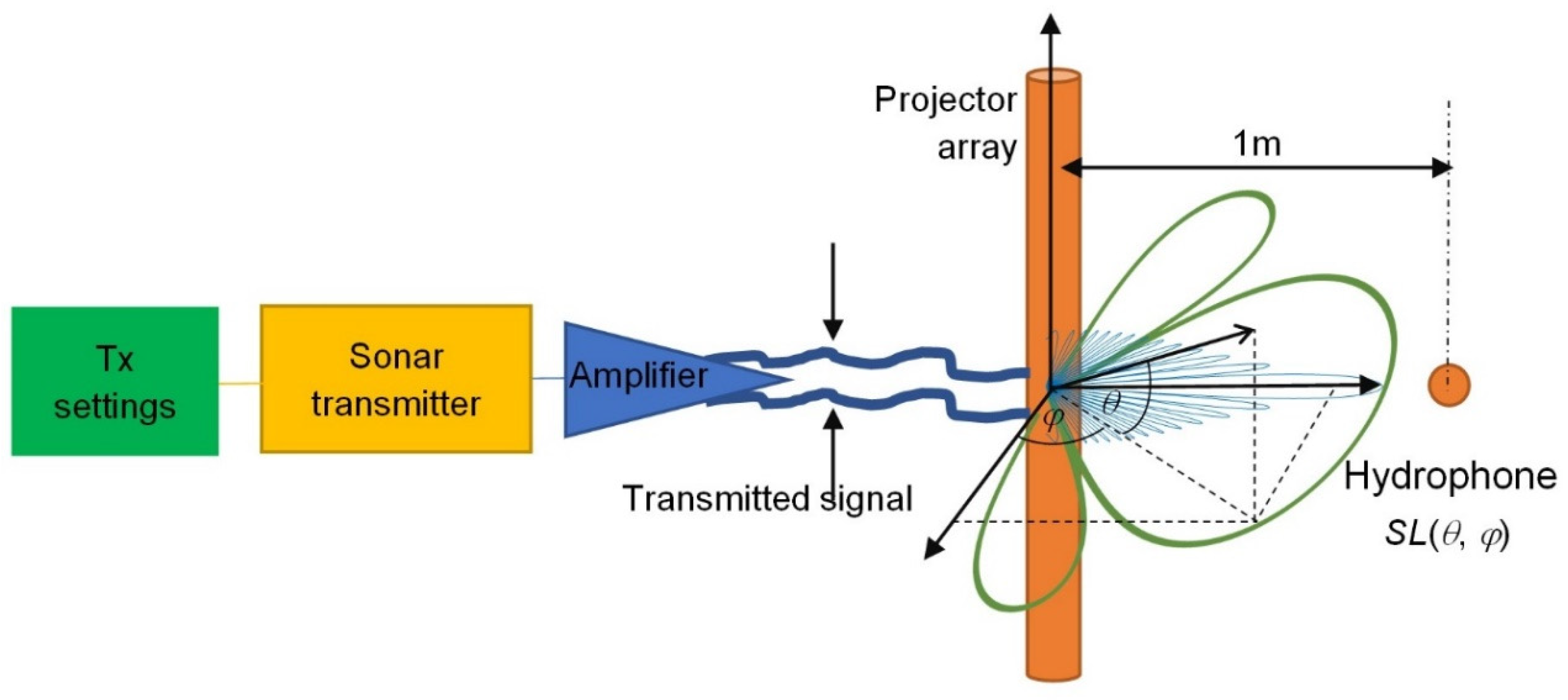
Figure 2 shows the transmitter path calibration setup. According to given Tx settings, the sounding pulse waveform is generated in the sonar transmitter segment and projected into the water column in the laboratory tank toward the hydrophones. The hydrophone pointed at (θ, φ) with respect to the center of the projector array registers the source level for this direction.

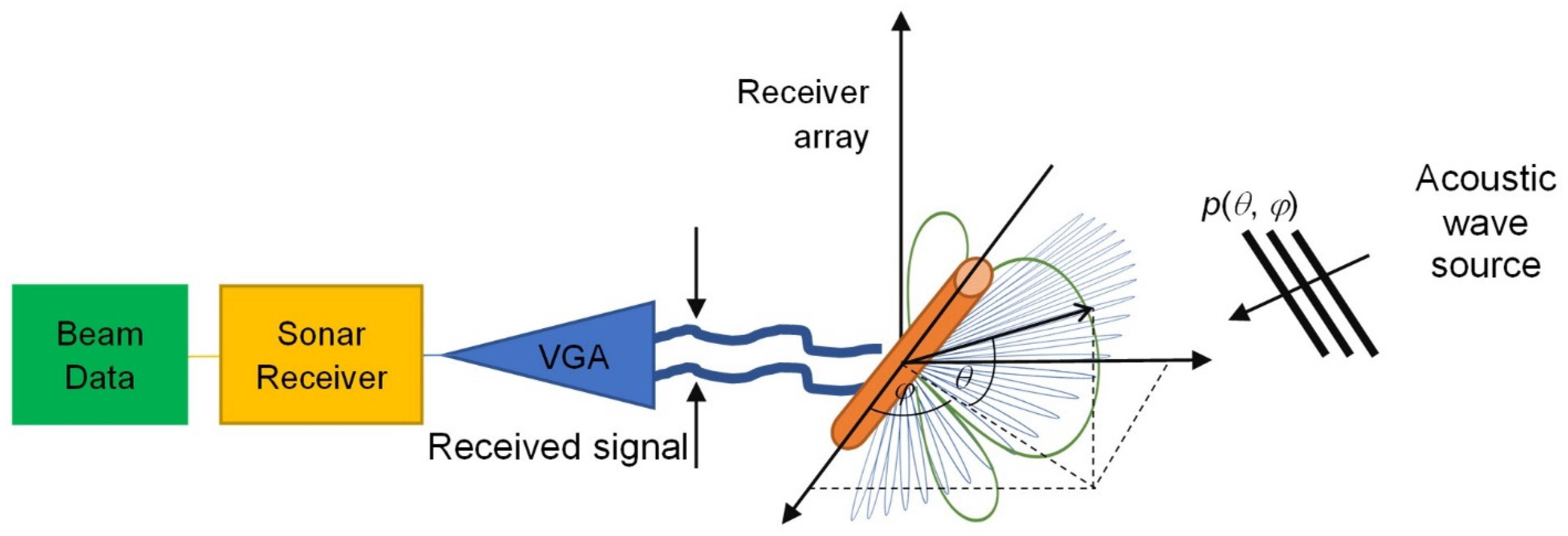
Figure 3 shows the receiver path calibration setup. The independent sound source pointed at (θ, φ) and situated at a given distance generates an acoustic wave of known characteristics p(θ, φ). After being received by the echosounder receiver array and transformed into the electric domain, then into digital form, the appropriate signal processing is done in the sonar receiver segment, including VGA, beamforming, and matched filter processing, resulting in beam data.

The quantities and characteristics measured during the calibration included the following:

• Source level (SL₀) of the transmitting sector Tx;
• Two-dimensional directivity patterns Dir_Tx and Dir_Rx for the set of transmitting and receiving transducers;
• Receiver sensitivity, including the antenna component OCR and the gains related to signal processing, VGA and PG;
• Actual characteristics of transmitted signals, i.e., pulse duration and shape.

The measurements were conducted in a wide range of transmitter settings and conditions, including power, frequency, pulse duration, and pulse type (continuous wave or chirp) with different bandwidths.

It should be noted that not all quantities mentioned in the above equations can be measured separately, but the complete results of measurements allowed us to evaluate and appropriately compensate for the joint influence of the sonar component characteristics on the obtained BBS values.

The calibration results described above were written in XML files, which were used by the NORBIT software to generate corrected records. The files contain all corrections of the system, such as multifrequency beam patterns, gains, and frequency responses for all parts of the system in the entire operating frequency range from 150 to 700 kHz. These data, along with the applied models of particular terms in the sonar equation, allow us to compensate for sonar characteristics and to base the bottom classification or habitat mapping on measurements of physical quantities such as backscattering strength.

2.2. Research Area and Data Collection

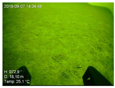
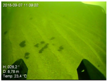
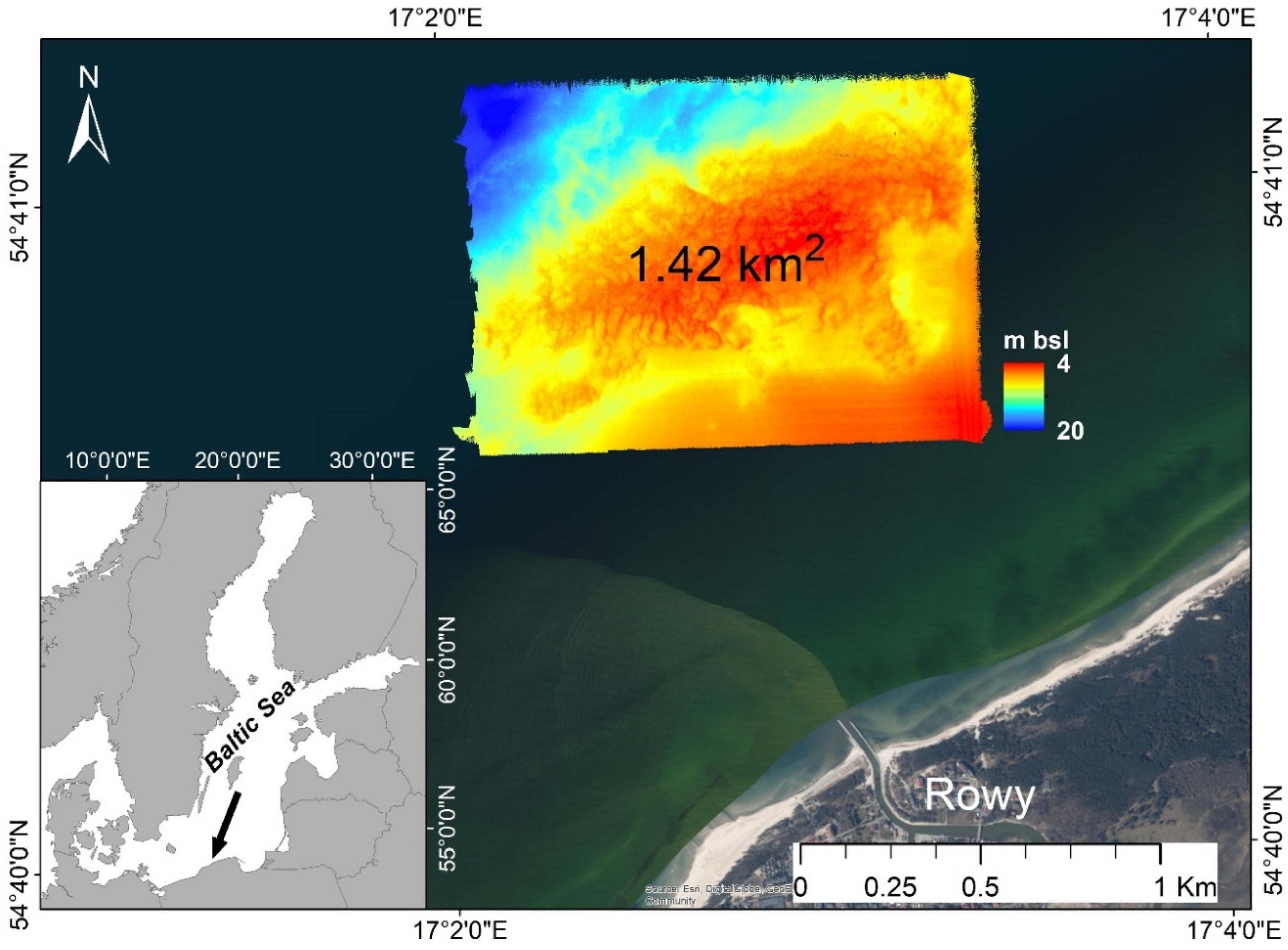
The measurements with the NORBIT MBES were conducted in the Rowy seafloor area, located approximately 1.5 km off the southern coast of the Baltic Sea (Figure 4). This area is characterized by post-glacial sedimentation and local current transport. The seafloor deepens from the coast toward the northwest with a gentle slope [8]. The study area in the central part is built by glacial till covered by boulders and pebbles. 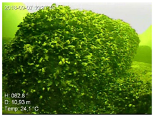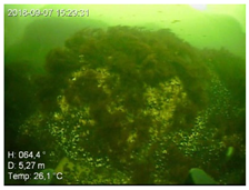In the southern and northwestern parts of the area, a cover of fine-grained sands occurs on the bottom surface (Figure 5). The research area ranges between 4 and 20 m water depth and is morphologically diverse. Numerous pebbles and boulders are covered with Mytilus trossulus bivalves [8,44]. In the study area, there are red algae, such as Bangiophyceae, including Furcellaria lumbricalis and Polysiphonia fucoides. The northwestern and southern parts of the area are relatively flat and covered with very fine sands [8] (Figure 5).

A test version of the NORBIT MBES was used during the measurements. The NORBIT iWBMSh STX is a compact, high-resolution, tightly integrated, broadband multibeam sonar with a curved array. Its small form factor, low power draw, and tight integration allow installation on any survey platform. The MBES was equipped with an integrated Applanix OceanMaster inertial navigation system (INS) with two Trimble antennas for the global navigation satellite system (GNSS) pole mounted on a frame attached to the side of the boat. Two GPS antennas were mounted on the roof of the boat cabin. We used real-time kinematic/global positioning system (RTK-GPS) corrections from the ASG-EUPOS NAWGEO service, with an accuracy of 3 cm horizontally and 5 cm vertically [45]. A Valeport sound velocity profiler was used to provide accurate profiles of the sound speed in the water column. The NORBIT iWBMSh is dedicated for use in shallow-water research between 0.2 and 160 m depth. It can collect 512 beams at frequencies ranging between 150 and 700 kHz. We used a swath coverage of 150–160° to maintain the density of our bottom detections. The maximum ping rate was 20 Hz. The measurements were made at a vessel speed of 3 m/s, and data were recorded in Qinsy software and NORBIT’s GUI software. To maintain homogeneous data density, the equiangle mode was used, i.e., a beamforming mode with a constant distance in angles between consecutive beams. We applied a pulse length of 200 µs for 150 kHz. At a frequency of 150 kHz, the receiving beam width is 2.4° × 2.4°, and, at the maximum available frequency of 700 kHz, it is 0.5° × 0.5°. A full patch test was conducted, and offsets were applied in order to achieve accurate positioning. Only acoustically calibrated iWBMSh STX MBES data were used to prepare the resulting ARCs in order to obtain absolute backscattering strength values.

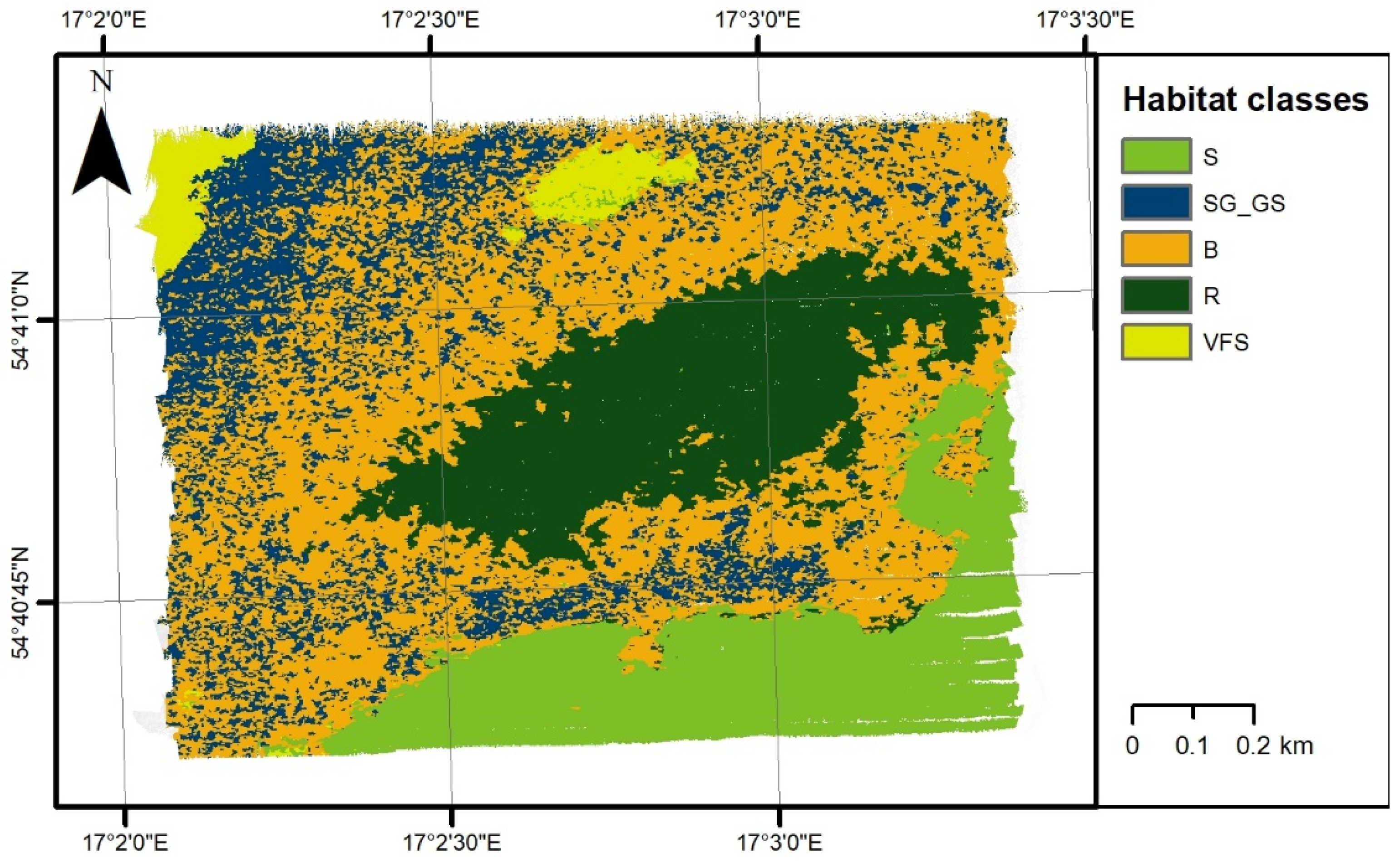
In the studied area, 57 samples of bottom sediments were collected [9], and benthic habitats were separated into five classes [46,47]: S, sand; SG-GS, sandy gravel or gravelly sand; B, boulders; R, red algae on boulders; VFS, very fine sand (Figure 5). The area was divided into six classes using object-based image analysis (OBIA) classification [8], presented in Figure 6. We also considered samples on artificial structures (wrecks), but since they were not representative in the later part of data analysis and statistics calculation, this class was omitted. Grab samples were collected from aboard the University of Gdansk research vessels Oceanograf and Zelint.

2.3. Postprocessing of Backscatter Data

Data were recorded in a shallow water area, and we applied environmental parameters 10 °C, 7 PSU, depth 0, and pH 8.

The data were replayed in the NORBIT GUI software applying the correction described in Section 2.1. The replayed BBS was corrected for acoustic absorption in the water body, where a constant absorption value of 15 dB/km for 150 kHz was calculated after Francois and Garrison’s equation [24].

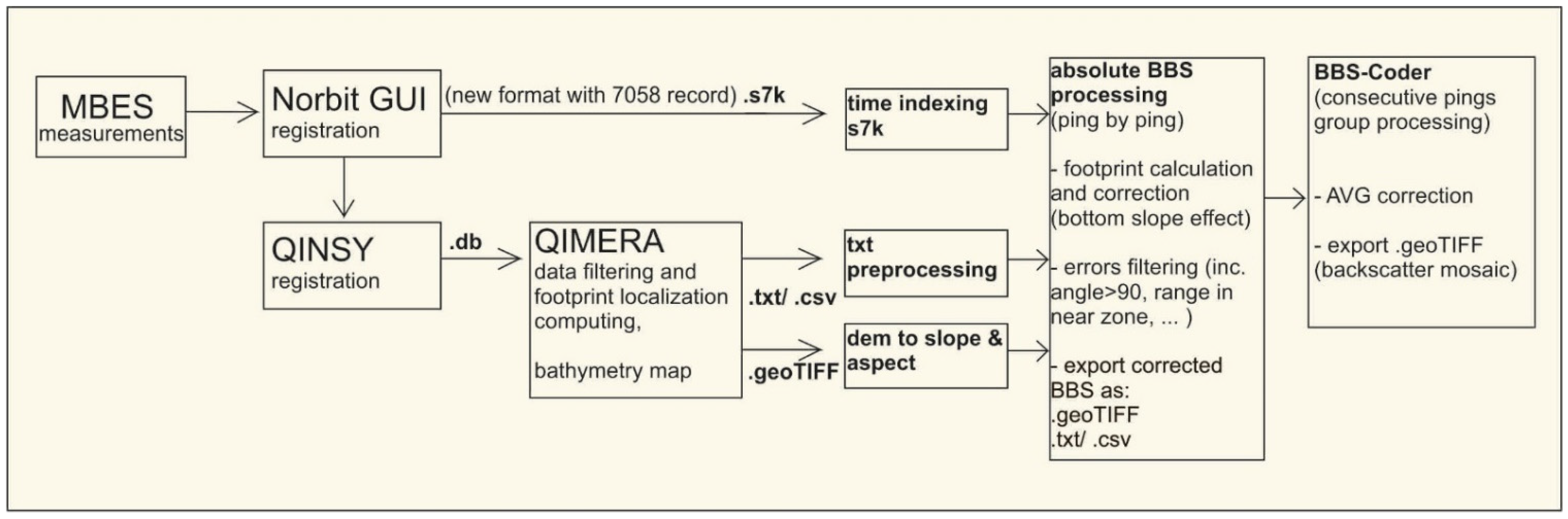
Bathymetry was processed in Qimera software with standard corrections, including ray path correction, cleaning and spike removal, and application of roll, pitch, and yaw offsets from calibration. Information about the position of each sounding for all pings was exported from Qimera as a txt file with a location in the UTM WGS 84 33N projected coordinate system. We developed our own software combining s7k (MBES data format) and txt files to access corrected BBS and position information (Figure 7). Then, we implemented a correction to compensate for the effect of a sloping seabed and true incidence on BBS in order to know the angular relationships of absolute BBS values for different types of seabed. First, we removed the correction used in the NORBIT GUI based on the flat bottom assumption correction from the calculated surface area A of the reverberation. Then, we adjusted the resulting values by our calculated BAC values (Equation (3)), where we considered the slope of the seafloor and the depth and distance from the transducer at each measurement point when calculating the reverberation area. These values were averaged and are presented in the results section as angular response curves of BBS values. In the next step, we ran our AVG correction, BBS-Coder, to remove the angular response as an intrinsic property of the seabed for the sake of generating a backscatter map that is easy to interpret and suitable for image-based classification. The correction algorithms were written in the D programming language [48].

2.3.1. Reverberation area and Bottom Slope Correction

The BBS value depends on the surface area A of the reverberation (Equations (2) and (3)). Significant changes in the BBS value are introduced by considering the actual distance of the acoustic transducer from the point measured at the bottom (R (range) in Equation (8)). The reverberation area on a flat bottom can be calculated from the angle of the receiving beam of the multibeam echosounder, the distance from the transducer to the bottom, and the angle of incidence. However, on a hummocky seabed, the true reverberation area can only be calculated in postprocessing after a 2D bathymetric model has been generated. In fact, the surface of the seabed is hardly ever perfectly flat, thus requiring calculation of the true angle of incidence. As a result, the individual beam reverberation area is not only controlled by the beam angle but also by the slope of the seabed. In order to calculate the reverberation area, it is necessary to consider the actual angle of incidence on the corrugated bottom and the angle of inclination of the bottom in relation to the transducer’s center beam of the sonar [49,50,51]. It is, therefore, necessary to use roll/pitch vessel movement correction to obtain a more precise calculation.

In our study, the roll/pitch vessel movement was applied in Qimera to set the ship’s location and orientation and to calculate the resulting positions of all soundings on the seabed. Seafloor slope was calculated using a bathymetric map with a resolution of 0.5 m, with most of the area, A, being less than 0.5 m². After the bathymetry was calculated, the received beam orientation of the survey was back-calculated again to obtain the true incidence of each beam on the tilted seafloor. For all recorded data and all angles of incidence, the reverberation area A was calculated, and further BBS was calculated using Equation (2). Consideration of the bottom slope gently changed the BBS values.

2.3.2. BBS-Coder: AVG Correction, and Backscatter Map Preparation

The backscattering strength recorded by the MBES depends on the angle of incidence of the acoustic pulse to the bottom. High BBS values near 0° incidence angles are primarily related to Lambert’s law describing characteristics of the backscattered sound, which depends on the cosine of the angle of incidence [31,42].

To implement BBS-Coder, we used the averaged values of the measured BBS in a sliding window with averaging of neighboring pings. All BBS measurements in the studied area were brought down to values corresponding to the backscattering for an angle of 40° in order to generate a uniform backscatter map. We selected 40° as the center of the far angular range defined by Fonseca and Mayer [52]. There is no standard for the choice of reference angle [12], but backscattering from 40° is less angle-variant and more distinct for discriminating between various benthic habitats; therefore, this is often the angle of reference. Fonseca et al. [32] used 20–30° and Lamarche et al. [27] chose 45° as the discriminant value.

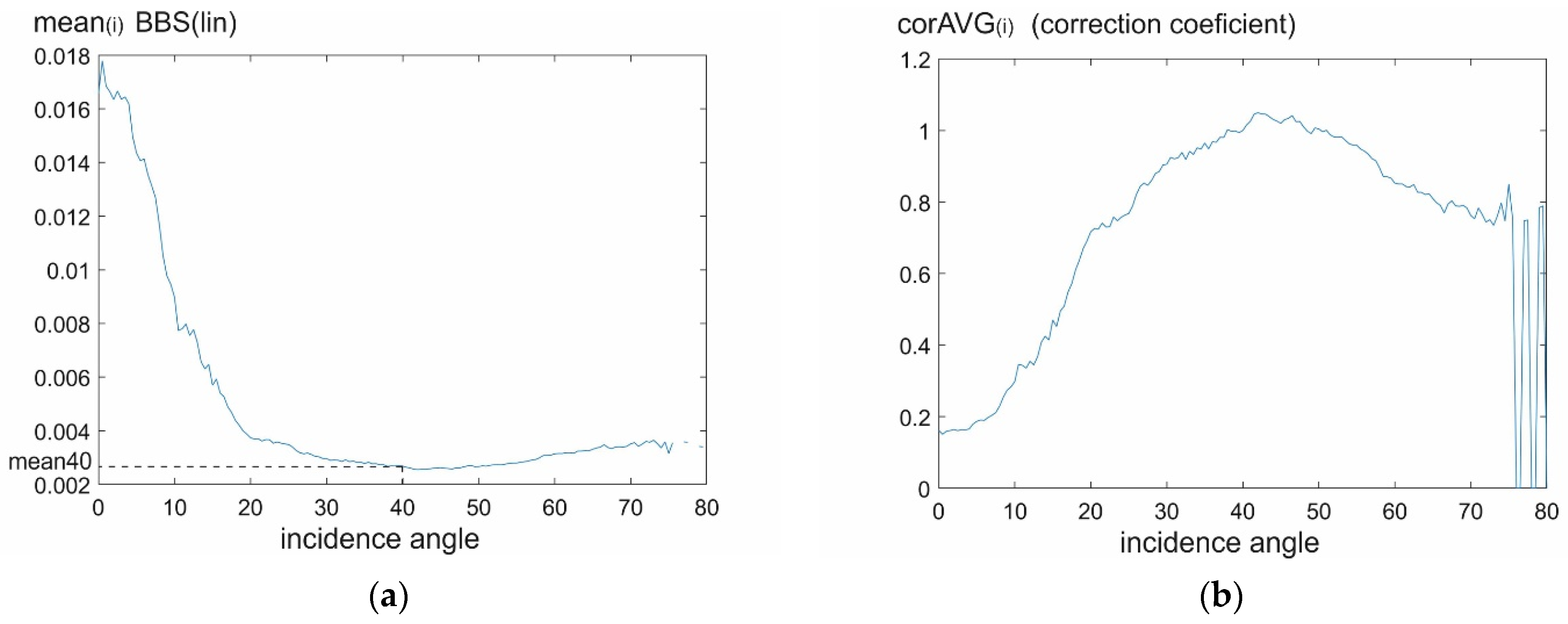
The applied BBS-Coder procedure was based on the division of recorded MBES data into subsets, with each subset containing a sequence of 50 pings, and each ping having 512 beams. It was assumed that the bottom backscattering properties were constant within each subset. From all recorded data in a given subset, we calculated the average BBS values for the angle of incidence, as shown in Figure 8a. Each registered beam was assigned to an appropriate half-degree interval of the angle of incidence (having a center value of 0°, 0.5°, 1°, 1.5°, 2°, 2.5°, etc.).

The correction coefficients, $corAV{G}_{\left(i\right)}$, were then calculated for each angle of incidence as follows:

$$corAV{G}_{\left(i\right)}=\frac{\mathrm{mean}40}{{\mathrm{mean}}_{\left(i\right)}},$$

(9)

where corAVG_(i) is the value of correction for i incidence angle, i = 0°, 0.5°, 1°, 1.5°, 2°, 2.5°, … 90°, mean40 is the average value of 10^(BBS/10) for an angle of incidence of 40°, and mean_(i) is the average value of 10^(BBS/10) for angle of incidence i.

Averaging and multiplication were performed for linear values.

An example of the correction coefficients calculated for one of the 50 ping packages is shown in Figure 8b. In the right part of Figure 8, we can see large changes in values; this is due to zero correction values for angles that were not present in the analyzed packet of 50 pings, as seen in Figure 8a. Then, each BBS value in the dataset (50 pings × 512 beams) was multiplied by the corAVG value appropriate for the angle of incidence of a given beam.

$$BS{40}_{\left(j\right)}=10lo{g}_{10}({10}^{\left(\raisebox{1ex}{$BB{S}_{\left(j\right)}$}\!\left/ \!\raisebox{-1ex}{$10$}\right.\right)} corAV{G}_{\left(i\right)}),$$

(10)

where BS40_(j) is the value after correction for j number of beams in the data package, j = 1, 2, 3, … 25,600 (50 pings × 512 beams). In fact, the maximum value of j is slightly lower because some of the measuring points were removed during the cleaning process.

Backscatter maps presented in the results section were generated from the calculated BS40 values. A single 0.5 × 0.5 m grid element often contains several calculated BS40 values. In such a situation, the values in a single grid element are averaged in order to prepare a map of the studied area.

3. Results

3.1. Angular Response Curves of BBS Values for Specific Habitat of the Baltic Sea

We calculated the angular response curves of absolute BBS for the specific habitat of the Baltic Sea occurring in the studied area: S, sand; SG-GS, sandy gravel or gravelly sand; B, boulders; R, red algae on boulders; VFS, very fine sand. Figure 9a shows the dependence of BBS on the angle of incidence, for which the values are averaged for the measurements made in the areas where homogeneous habitats occur, according to the separations from the map of habitats according to Janowski et al. [8] (Figure 6) for 150 kHz. Figure 9b shows the angular response curves of BBS values. The values are averaged for measurements made within a 3 m radius of the sampling points for 150 kHz.

Table 1 presents the acoustic characteristics of habitat types occurring in the research area. The dependence of BBS values on the angle of incidence was determined for two situations:

• Black line: angular response curves of BBS with values averaged for measurements made within 3 m radius of the sampling points for registration using 150 kHz signal frequency;
• Dashed black line: angular response curves of BBS with values averaged for measurements made in areas where homogeneous habitats occur, according to the separations from the map of habitats according to Janowski et al. [8] (Figure 6) for registration using 150 kHz signal frequency.

Table 1. Angular response curves of BBS: black line, 150 kHz, data from samples; dashed black line, 150 kHz, data from object-based image classification.

Class ID	BBS (dB) 150 kHz	Seabed Image/Composition
VFS		Bare, flat area of very fine sand with worm burrows
S		Sand or slightly gravelly sand with ripple marks
SG-GS		Sandy gravel or gravelly sand, rare boulders with barnacles and Mytilus trossulus
B		High concentration of Mytilus trossulus on dense boulder substratum
R		Large dense patches of red algae with a high concentration of Mytilus trossulus on boulder substratum

Table 1. Angular response curves of BBS: black line, 150 kHz, data from samples; dashed black line, 150 kHz, data from object-based image classification.

Class ID	BBS (dB) 150 kHz	Seabed Image/Composition
VFS		Bare, flat area of very fine sand with worm burrows
S		Sand or slightly gravelly sand with ripple marks
SG-GS		Sandy gravel or gravelly sand, rare boulders with barnacles and Mytilus trossulus
B		High concentration of Mytilus trossulus on dense boulder substratum
R		Large dense patches of red algae with a high concentration of Mytilus trossulus on boulder substratum

Figure 9 and Table 1 present the angular response curves of absolute BBS. Close to an angle of 80°, there were large fluctuations in the values, because, in the extreme part of the swath, fewer measuring points were recorded in equiangle mode, many points from the outer beams were rejected in the cleaning process, and the values from the individual registered measuring points varied considerably. Figure 9a,b do not perfectly show the BBS relationships for the given benthic habitats. Figure 9a presents BBS values averaged within the habitat classes, whose boundaries were determined in a semi-automatic classification process; hence, they are not perfectly defined despite having high classification accuracy. Figure 9b presents BBS values averaged within 3 m radius circles around the ground-truth data, which is a theoretical assumption, because there can also be other habitats present in these buffers.

3.2. Backscatter Maps: BBS-Coder Result

Figure 10 shows backscatter value maps prepared in this study for registration using 150 kHz signal frequency. Figure 10A presents backscatter mosaic grids with relative backscatter values without angular (AVG) and bottom slope (BAC) correction. The near 0° incidence angle showed the strongest signals and also the fastest drop-off. Figure 10B was created with the manufacturer’s MBES calibration (NORBIT) and bottom slope correction (correction of reverberation area, which is improved by bottom slope and calculated range) but without our AVG correction. Figure 10C was created with the manufacturer’s calibration (NORBIT), bottom slope correction, and the BBS-Coder AVG correction developed in this study and described in Section 2.3.2. The near 0° incidence angle represented the strongest signal fluctuations.

4. Discussion

Calibrating the MBES makes it possible to obtain absolute values of BBS, which is an essential feature for specific geoacoustic settings on the seabed and benthic habitats and very helpful in distinguishing them. Only a few studies with absolute BBS have been reported due to technical difficulties associated with MBES calibration and post-measurement data correction; moreover, MBES studies with resulting ARCs are extremely sparse [13,16].

Any physically correct calibration method improves data quality and provides valuable information. The technology now developed for working with MBES makes it possible to fully calibrate the instrument, and the validity and usefulness of the absolute BBS values make it necessary to always use calibrated echosounders.

Several papers have already been written showing absolute BBS values recorded by MBES for bottom habitats. Eleftherakis et al. [16] performed a calibration of the backscatter strength values recorded by MBES with reference to data recorded in the same place by an acoustically calibrated single-beam echosounder (SBES). They presented the dependence of backscatter strength on the angle of incidence in three research areas with different types of sediment at 200 and 333 kHz. Wendelboe [13] presented average values of seabed backscattering strength obtained in the frequency range from 190 to 400 kHz, for grazing angles from 20° to 90°. This study showed that seabed backscattering strength ranged from −8.5 to −19 dB for 400 kHz and from −13.5 to −23 dB for 200 kHz. Weber and Ward [15] took measurements with a calibrated SBES at 170 and 250 kHz in an area with sand, gravel, and bedrock seafloor. Williams et al. [14] measured backscattering at frequencies of 20–150 kHz with grazing angles of 20–30°, and, in subsequent work [17], they measured backscattering at frequencies of 200–500 kHz with grazing angles of 32° and 42°. They recorded increasing values with increased frequency. Stanic et al. [18] performed acoustic bottom backscattering measurements east of Jacksonville, Florida, and recorded data from sidescan sonar. Measurements were made in a coarse shelly area with frequencies of 20–180 kHz and grazing angles of 5–30°. It was found that backscattering strength values slightly decreased with increasing frequency.

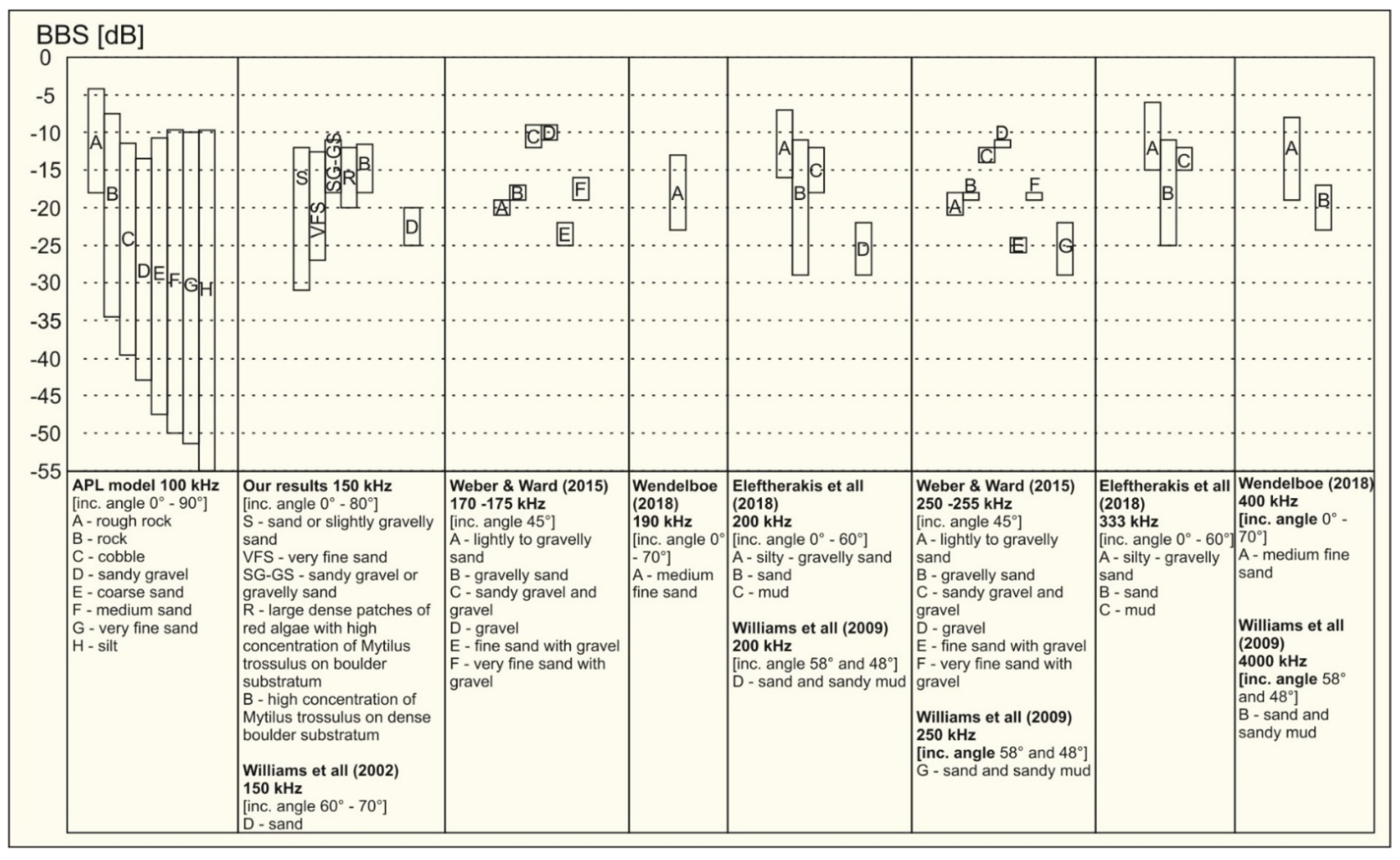
To compare our results on BBS measurements with those recently reported by other researchers, we summarized the basic information on the particular works in Figure 11. In general, the results obtained in this work on the dependence of BBS on the angle of incidence are in line with those achieved by other authors who performed MBES measurements [16,32], as well as the theoretical predictions.

It is difficult to compare data recorded by different authors because there are few papers and the benthic habitats studied vary; however, the BBS values we obtained for sand are similar to those obtained at 60–70° incidence angle and 150 kHz by Williams et al. [14] and to those using the APL model at 100 kHz [29]. The values presented for S (−12 to −31 dB) and VFS (−12.5 to −27 dB) are similar to those of Eleftherakis et al. [16] in the Camaret area with sand (−11 to −29 dB at 200 kHz); the values for SG-GS (−10.5 to −18 dB) are similar to data in the Carré Renard area [16] with silty–gravelly sand (−7 to −17 dB at 200 kHz); the values for R (−12 to −20 dB) and B (−11.5 to −18 dB) are similar to data in the Aulne area [16] with mud (−12 to −18 dB at 200 kHz).

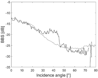
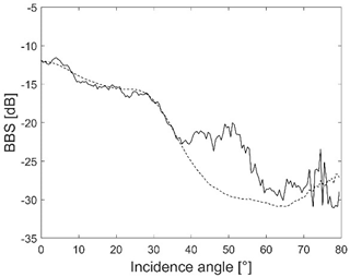
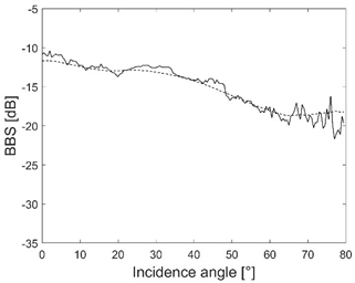
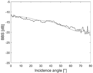
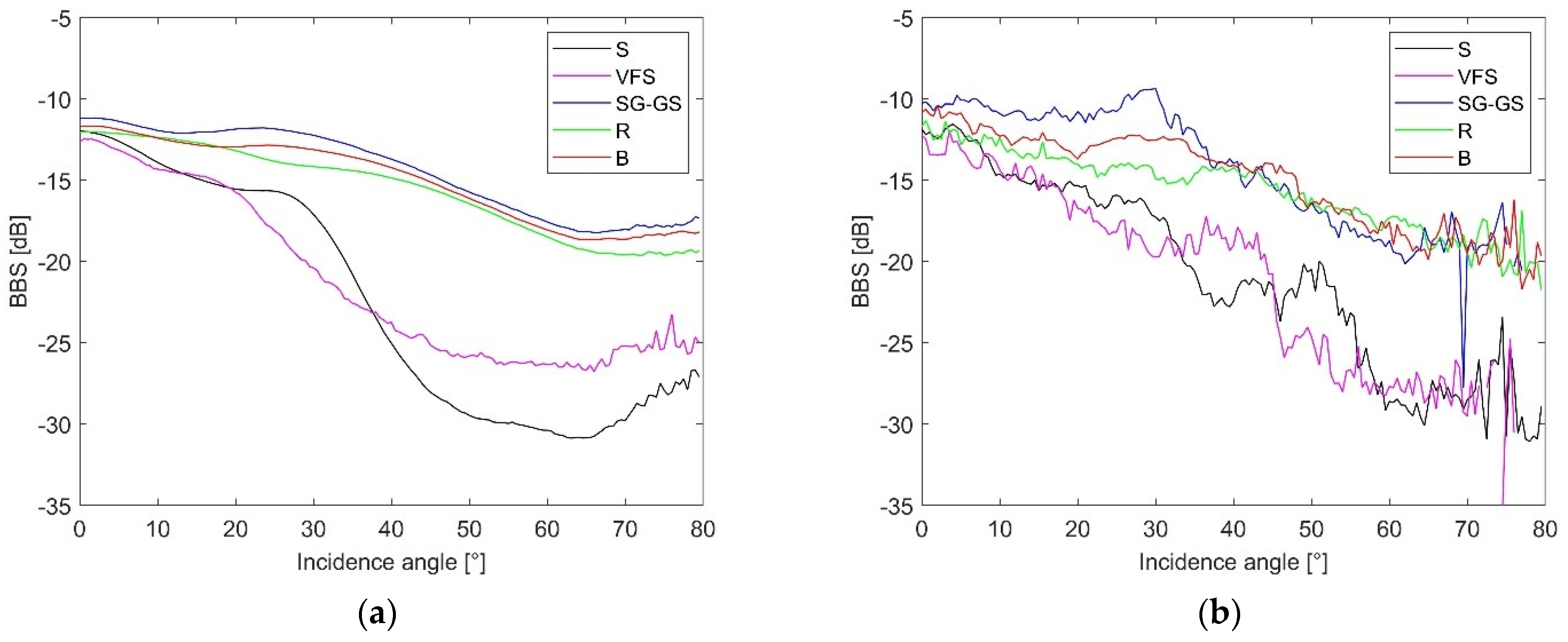
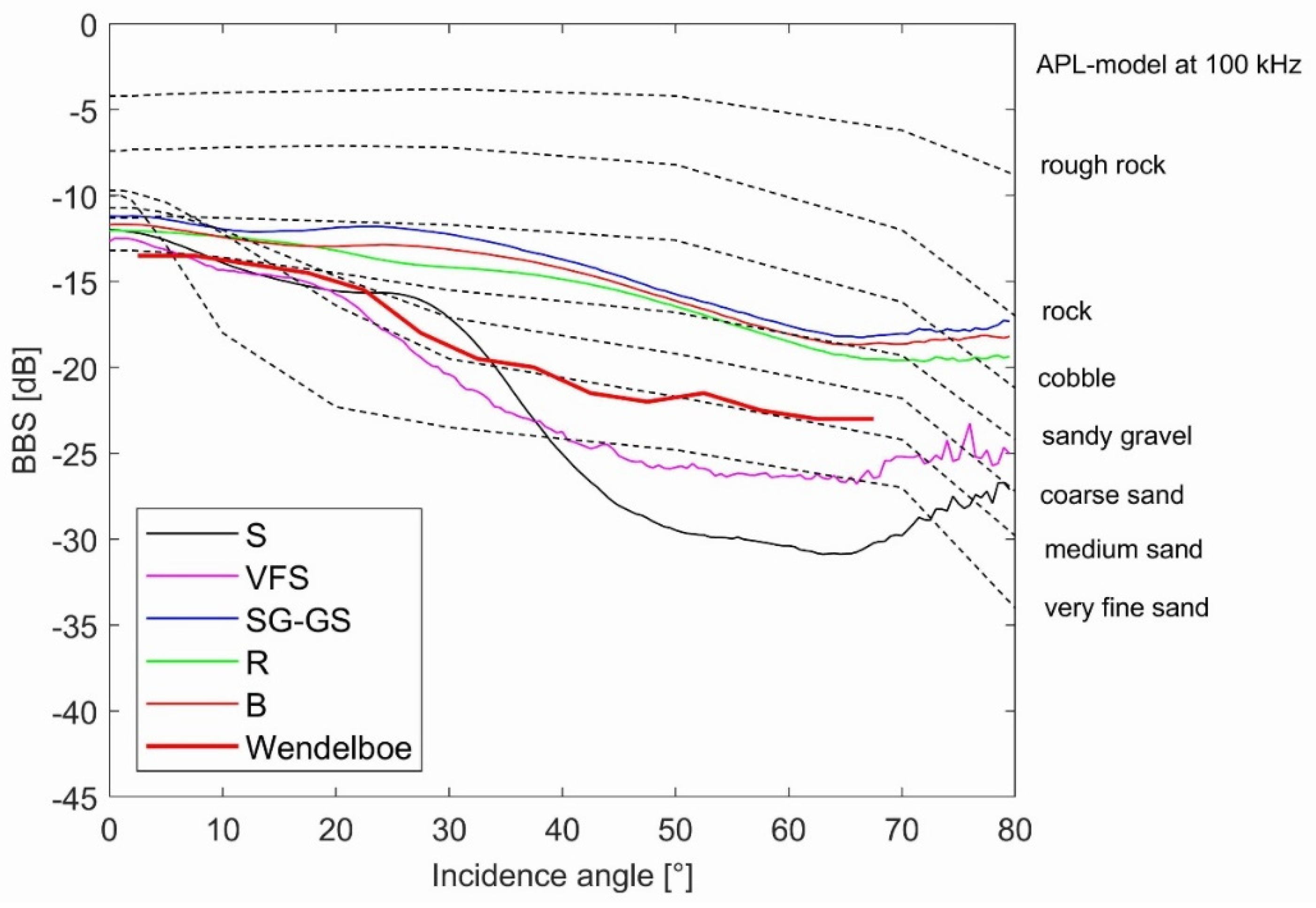
The BBS for S and VFS has similar values and angular relationships (Figure 12) to seabed backscattering strength values presented by Wendelboe [13] obtained at a frequency of 190 kHz for medium–fine sand. For the entire angular range, the BBS for SG-GS, R, and B reaches higher values than for S and VFS. Habitats S and VFS have a characteristic shape typical of the ARC curve of fine-grained sediments in the APL model (Figure 12). In contrast, the SG-GS, R, and B habitats have a characteristic shape typical of the ARC curve of acoustically hard sediment such as rock in the APL model at 100 kHz (Figure 12). Habitats SG-GS, R, and B achieve similar BBS values to sandy gravel and cobble in the APL model at 100 kHz. For incidence angles from 25° to 65°, the ARC curve showed a significant decrease in value greater than the APL model at 100 kHz, and this may be related to the higher frequency of the tested signal, 150 kHz.

In the summary of BBS values obtained by researchers, it is difficult to see a trend of increasing value with increasing frequency. However, such a trend was indicated in some studies that considered different frequencies [14,17]. Williams et al. [14,17] suggested that, at high frequencies, scattering from large fragments of shells is dominated by a different scattering mechanism than surface or volume scattering. Weber and Ward [15] recorded a weak increase in backscattering strength with increased frequency for moderately well-sorted medium sand and a slight decrease in all other locations. In many places, higher backscattering strength values were recorded for 170 kHz than for 250 kHz (as shown in Figures 6 and 7 in [15]). Weber and Ward [8] speculated that the maximum backscattering strength existed at a frequency lower than what they tested (below 170 kHz), and that backscattering strength may be connected with some characteristic length scale via which diffuse scattering reaches a maximum for this type of sediment [15].

Roughness is a matter of the wavelength of the acoustic pulse and the size of bottom irregularity. For one and the same seafloor, in the case of high frequencies, the bottom may appear rough, while, for low frequencies, the bottom acoustically behaves like a smooth seafloor, all determined by the Rayleigh parameter [53].

We suggest that the higher BBS values for higher frequencies are associated with strong scattering of higher-frequency signals on an rough seafloor surface [53].

In the ARC curves presented here, the sand habitat (S) showed that an increase in BBS value around 30° incidence is not in line with the APL model curve. This may be due to the presence of sand ripple marks in the study area, similar to Lurton et al. [54]. Although BBS values were corrected for the slope of the seabed, irregularities less than 1 m can still be significant. Seabed slope was calculated using a bathymetric map with 0.5 m resolution; however, from an acoustic and snippet backscattering perspective, modulation of the backscattering strength through microroughness becomes likely. In addition, local grain size changes were noted in the study area where ripple marks occurred on ridges with fine-grained sand and in valleys with coarse-grained sand, which we believe affected the recorded BBS values.

The differences in Figure 9 and Figure 10 between the angular relationships of BBS values obtained from (a) averaging of habitat classifications and (b) ground-truth samples are more visible for habitat types VFS and S than for SG-GS, B, and R. This may mean that the latter three bottom types are more specific, and that the areas they include are more homogeneous. Habitat types VFS and S are more general and may include areas with different characteristics (different sediment/habitat types could have been assigned to them, both in the course of classification and in the 3 m areas around the cores).

For flatter bottom types (VFS, S) there is a large drop in BBS with increased deviation of the direction of the wave from the vertical, and, for cases with more irregular structure/shape (SG-GS, B, R), this drop is smaller. This is due to the low rate of diffusion scattering on the bottom surface, which usually dominates at large incidence angles.

Fonseca et al. [32] provided information on backscatter strength for 95–98 kHz frequency. According to the division of bands introduced by Fonseca et al. [32], the near range includes incident angles from 0° to 25°, the far range includes incident angles from 25° to 55°, and the outer range includes incident angles from 55° to 85°. In our data, we noted the occurrence of three similar zones from 0° to 25° with a weak slope of the curve, from 25° to 65° with a significant slope, and from 65° to 80° with a weak slope. However, high variability of habitats within the half-swath remains a problem for the method described by Fonseca et al. A possible future workaround could be to use automatic segmentation methods to determine the boundaries of individual habitats.

Unadjusted backscatter values have been successfully used for many purposes, including habitat classification [8,19,20,21]. For more advanced environmental analyses, such as studies of diurnal and seasonal variability of the seabed itself and seagrass scattering variation over time, it might be necessary to work with absolute BBS, because a few dB can determine the variability, as has been demonstrated [55]. Furthermore, the use of absolute BBS is necessary to compare results from different areas recorded at different times. Although the habitats are apparently similar, there are significant differences in their BBS. Sand in the Mediterranean Sea may have different BBS values than sand in the Baltic Sea because they have different physical properties. Habitats with similar physical properties (e.g., number and size of air bubbles in sediment, density) will have similar values. BBS is an intrinsic property of the seafloor and the prevailing habitat (not the multibeam echosounder); thus, it might be better to look for specific habitat-related features that can facilitate habitat recognition. Habitats and their BBS are very different from each other, and substantial research is necessary to know the scattering values of each habitat.

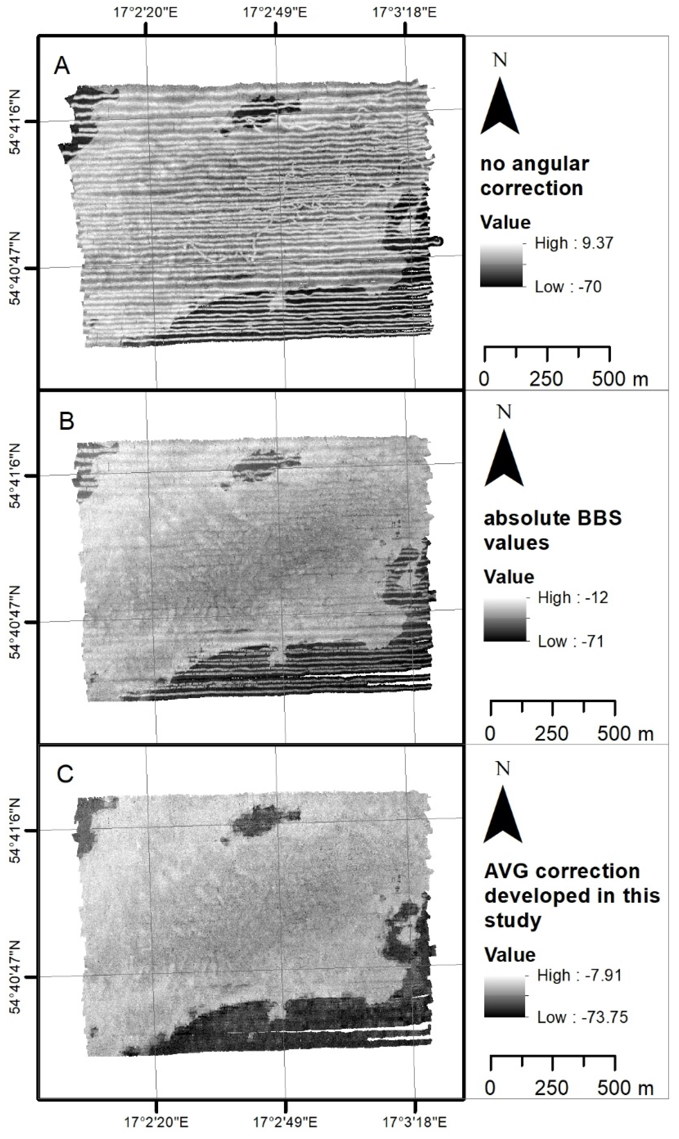
For automatic classification, e.g., object-based (OBIA) or texture (GLCM) analyses, backscatter maps reduced to a single incident angle are needed. There are few techniques for this correction. The methods used range from simple Lambert correction to complex models such as Geocoder. Due to the strong near-nadir errors in the mosaics prepared with the help of Geocoder, we developed our own correction method. It removes the influence of the incidence angle and brings the backscattering strength to an incidence angle of our choice (in this case, 40°).

Other useful backscatter mosaics with smoothed backscatter outcomes without angular dependency can be created using Geocoder [22]. The near 0° incidence angle represents a stronger signal standard deviation. Median filtering of BSS near the 0° incidence angle might be a good solution. Geocoder assigns quality flags to backscatter samples. Data samples closer to and further from the nadir have low values, while samples in the middle range have higher values and a greater influence on the final backscatter mosaic [22]. When our MBES data were recorded with a large overlap, all values found in the raster grid were averaged to generate the mosaic. The BBS-Coder presented here is less complex than the current Geocoder in FMGT QPS software; it is simple and effective, and it will be freely available on the ECOMAP project website (https://www.bonus-ecomap.eu/, accessed on 1 January 2021). The AVG correction scheme presented in this paper assumes the use of a radiometric and geometric correction tool (in this case, QPS Qimera software).

5. Conclusions

The continuous development of measurement technology provides new opportunities for seabed identification and mapping, as exemplified by the real BBS values presented here gathered with a modern GNSS-guided MBES. The absolute BBS should be used to describe habitats precisely, by a physically defined parameter. In the future, this may affect the way acoustic measurements are conducted by reducing the number of samples required to classify benthic habitats and making it easier to compare the scattering of acoustic signals on the bottom in different seasons.

This paper presented the angular dependence of BBS measurement results for several benthic habitats in the Baltic Sea at 150 kHz. The methods of correction used to measure the absolute value of the angular dependence of BBS included laboratory tank calibration, seabed slope correction, and the AVG correction developed in the work, and examples of the obtained mosaics as a result of the applied corrections (BBS-Coder) were shown. The BBS values obtained were −12 to −31 dB for sand (S), −12.5 to −27 dB for very fine sand (VFS), −10.5 to −18 dB for sandy gravel or gravelly sand (SG-GS), −12 to −20 dB for red algae on boulders (R), and −11.5 to −18 dB boulders (B). The AVG correction method presented is a simple and effective tool for preparing a backscatter mosaic useful for seafloor habitat classification.

For the entire angular range, the BBS values obtained for SG-GS, R, and B were higher than those for S and VFS. Habitats S and VFS had characteristic shapes typical of the ARC curve of fine-grained sediment in the APL model (Figure 12).

Examples of measurements presented by different studies suggest high variability of BBS. This may be related to variation within a single habitat, which, in different basins, may have different physical characteristics that vary with time of day and season. It is necessary to find the limits of BBS for specific habitats in specific basins according to numerous empirical studies.

Visual assessment of backscatter mosaic grids created using our methods shows their usefulness for further application, such as sustainable management of seabed resources, exploration of the sea bottom, benthic habitat mapping, and geological mapping of the seabed. The results presented were obtained using the NORBIT echosounder and software, which will be made available on the website associated with the ECOMAP project.

Corrected BBS values are very useful for the characterization of benthic habitats based on acoustic dependence characteristics. Their differentiation based on acoustic signatures may help to classify seabed properties only by specific acoustic responses. It may help to increase the importance of noninvasive underwater acoustic research, reducing the number of sediment ground-truth samples and expanding the classification of known benthic habitats for newly explored areas. However, it should be underlined that this kind of quantitative characterization of the seafloor substrate requires corrected BBS values [23,27]. Advances in calibrated multibeam echosounders are still in the development phase; however, thanks to recent advances by manufacturers, several MBES models calibrated in a test tank are now available. This provides an opportunity for habitat mapping and monitoring using the absolute response of the seafloor to backscattering, as well as its changes over time. We recommend measuring BBS using an acoustically calibrated echosounder and using such data to classify benthic habitats.