Estimating Local Inequality from Nighttime Lights

Abstract

Economic inequality at the local level has been shown to be an important predictor of people’s political perceptions and preferences. However, research on these questions is hampered by the fact that local inequality is difficult to measure and systematic data collections are rare, in particular in countries of the Global South. We propose a new measure of local inequality derived from nighttime light (NTL) emissions data. Our measure corresponds to the local inequality in per capita nighttime light emissions, using VIIRS-derived nighttime light emissions data and spatial population data from WorldPop. We validate our estimates using local inequality estimates from the Demographic and Health Surveys (DHS) for a sample of African countries. Our results show that nightlight-based inequality estimates correspond well to those derived from survey data, and that the relationship is not due to structural factors such as differences between urban and rural regions. We also present predictive results, where we approximate the (survey-based) level of local inequality with our nighttime light indicator. This illustrates how our approach can be used for new cases where no other data are available.

1. Introduction

In the social sciences, there is an increasing trend to use fine-grained data to capture political and economic mechanisms. Measured at high levels of resolution such as individuals or households, they allow for a precise analysis of local conditions and the social processes that people are embedded in [1]. The availability of fine-grained data is usually very good for developed countries, where researchers can rely on extensive surveys or administrative data. For many countries of the Global South, however, the availability of disaggregated data is usually limited. Oftentimes, these countries are unlikely to be covered by surveys, and administrative data shared for research purposes is sparse or does not exist.

For this reason, social science scholars have increasingly turned to alternative sources of data, such as remote sensing. One prominent example in this strand of research is the use of nighttime lights (NTL) data collected by satellites. First attempts have used NTL emissions at aggregated, lower levels of resolution. For example, earlier work has shown that nighttime light emissions can track economic performance and human development at the level of large geographic units, for example countries or states [2,3,4,5]. However, more recent work has tried to increase the resolution of these tests. For example, Weidmann and Schutte [6] show that nighttime light emissions correlate well with ground truth measurements of household wealth, as recorded in surveys. This means that satellite-based NTL data can be used also at high levels of resolution, for example for the estimation of wealth, human development or regional inequality between provinces and sub-national administrative units [7,8,9,10,11].

In this paper, we build on this work and attempt to use NTL data for the estimation of local inequality. In recent years, and in particular following the influential work by Piketty [12], inequality has attracted a lot of interest from the research community. Using aggregated country- or group-levels measures of economic inequality, this research has shown for example that inequality can be an important driver of social conflict and political instability [13]. Again, research in this vein has relied on NTL data, but only at aggregated levels to measure inequality between [14,15,16] or within social groups [17]. However, recent research has also shown that people do not perceive aggregated/systemic levels of inequality. Rather, it is the local context that matters for explaining individuals’ behavior. In particular, there is a number of studies showing that local inequality, i.e., inequality with an individual’s immediate spatial context, affects citizen’s political preferences in behavior [18,19,20,21,22,23,24].

To find out how this local context matters in the Global South, we need fine-grained estimates of local inequality. This is what we present in this article. Our study, however, is not the first to study local inequality with NTL data. Existing work, however, has not used night light emissions to measure local inequality directly; rather, these studies first approximate economic performance or wealth from night lights for small geographic units, and then calculate inequality between them [9,25,26]. Our approach, in contrast, operates directly on the NTL data in combination with a population raster, and is therefore able to produce local inequality estimates for arbitrary locations on the globe and at a high levels of resolution.

2. Data and Methods

In this paper, we present an approach to computing satellite-based estimates of local inequality, which we validate with local inequality estimates derived from large-scale survey data. In the following, we first describe the nighttime light data we use for our indicator, before turning to the survey data used for validation.

Our satellite-based estimates of local inequality rely on the VIIRS nighttime light data [27] (V2). We use the annual composites, where non-stationary light sources and other erroneous influences have been removed by a combination of the different images available for a given year. This methodology is described in Elvidge et al. [27]. The VIIRS nighttime lights is one of the most recent freely available data products of remote-sensed nighttime light emissions, and it is available for the years 2012–2021. Compared to earlier products such as the frequently-used DMSP-OLS nighttime light data [28], it has a number of advantages. Most importantly, VIIRS nighttime light rasters have a higher resolution of 15 arc-seconds, which corresponds to about 500m at the equator. Furthermore, VIIRS reduce the problem of top-coding: in the DMSP-OLS NTL data, high emissions are all coded at the maximum value of 63, which eliminates a lot of variation at the upper end of the spectrum. Therefore, with VIIRS data, we can exploit considerably more variation within well-lit areas. Not surprisingly, existing research has concluded that VIIRS-derived data should be preferred for work that uses nighttime lights to study socio-economic processes [29,30].

For our approach, we rely on earlier work by Weidmann and Schutte [6], which has analyzed nighttime light emissions as a proxy for economic wealth at high levels of resolution. This work has shown that on average, more intensely illuminated areas are also the richer ones. However, since variation in illumination to a large extent driven by settlement patterns, more populated areas emit more light at night. In our analysis, we take this into account by using a second spatial data source that maps the global population at a high resolution: the WorldPop dataset, available from https://www.worldpop.org/ (accessed on 30 July 2021) [31]. We use the population counts raster from WorldPop, which provides annual population estimates at the level of cells with a resolution of 30 arc-seconds. These counts are computed in a “top-down” fashion, by disaggregating official population statistics for administrative divisions using spatial covariates as described in Lloyd et al. [32].

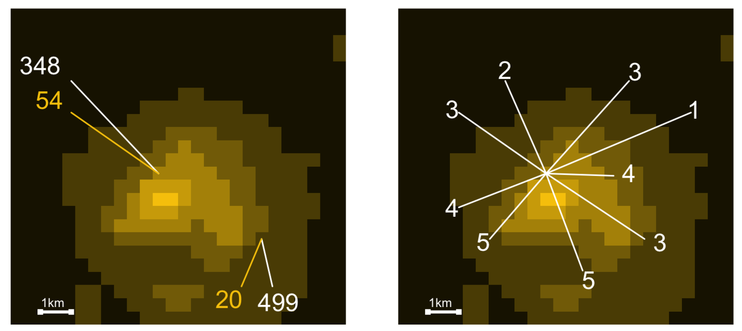
For combining the VIIRS NTL data and WorldPop, we aggregate the former to a resolution of 30 arc seconds. Dividing the nighttime light emissions value by the population living in the same cell, we obtain per capita values of nighttime light emissions at the level of the raster cells. This allows us to compute inequality estimates for any given point on the globe: Given a set of longitude/latitude coordinates, we retrieve all cells within a buffer of a certain radius, and simply compute an inequality index—the Gini coefficient—across all of them. For this computation, we need the per capita nighttime light emissions as well as the population counts of each grid cell. 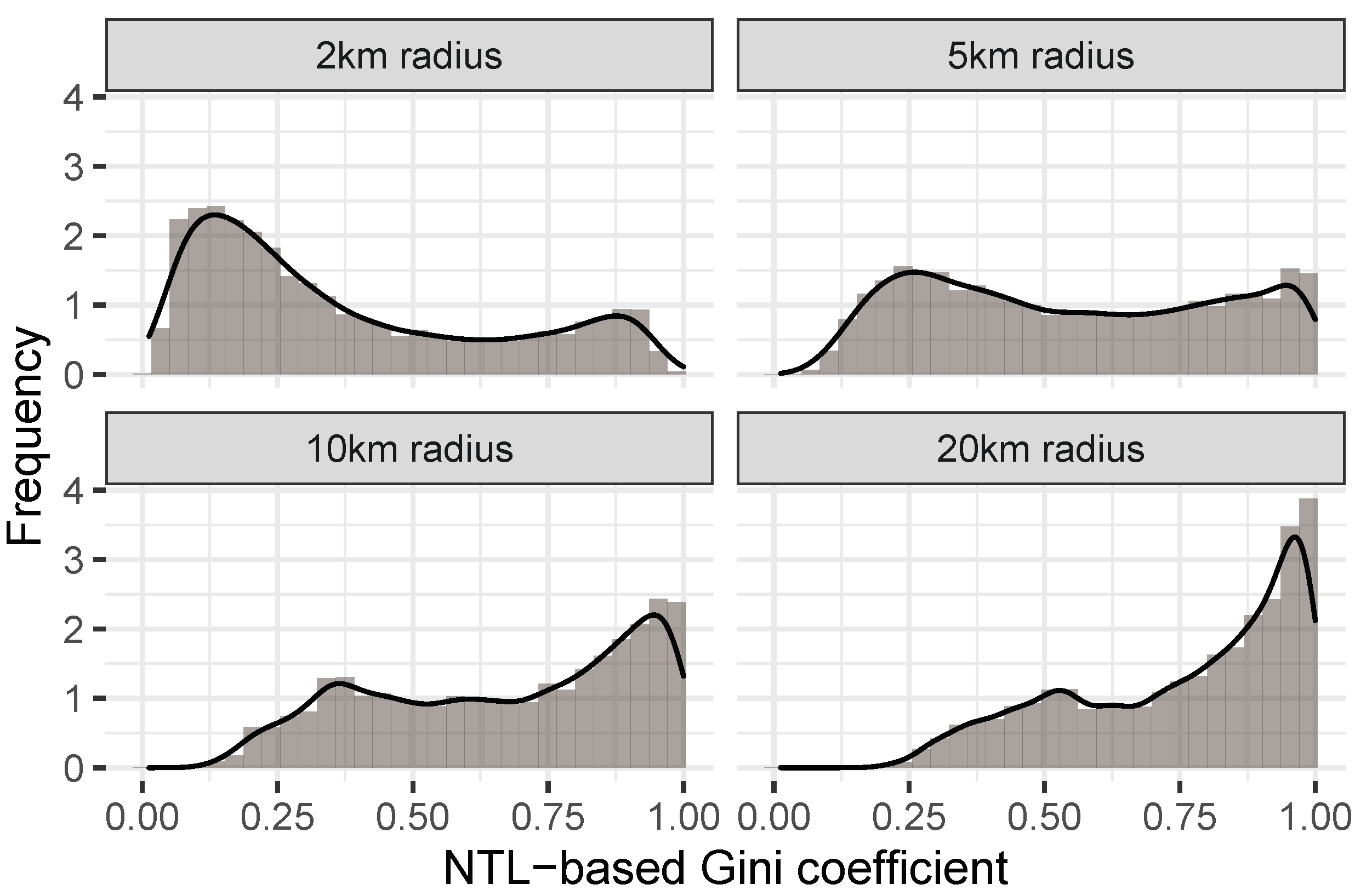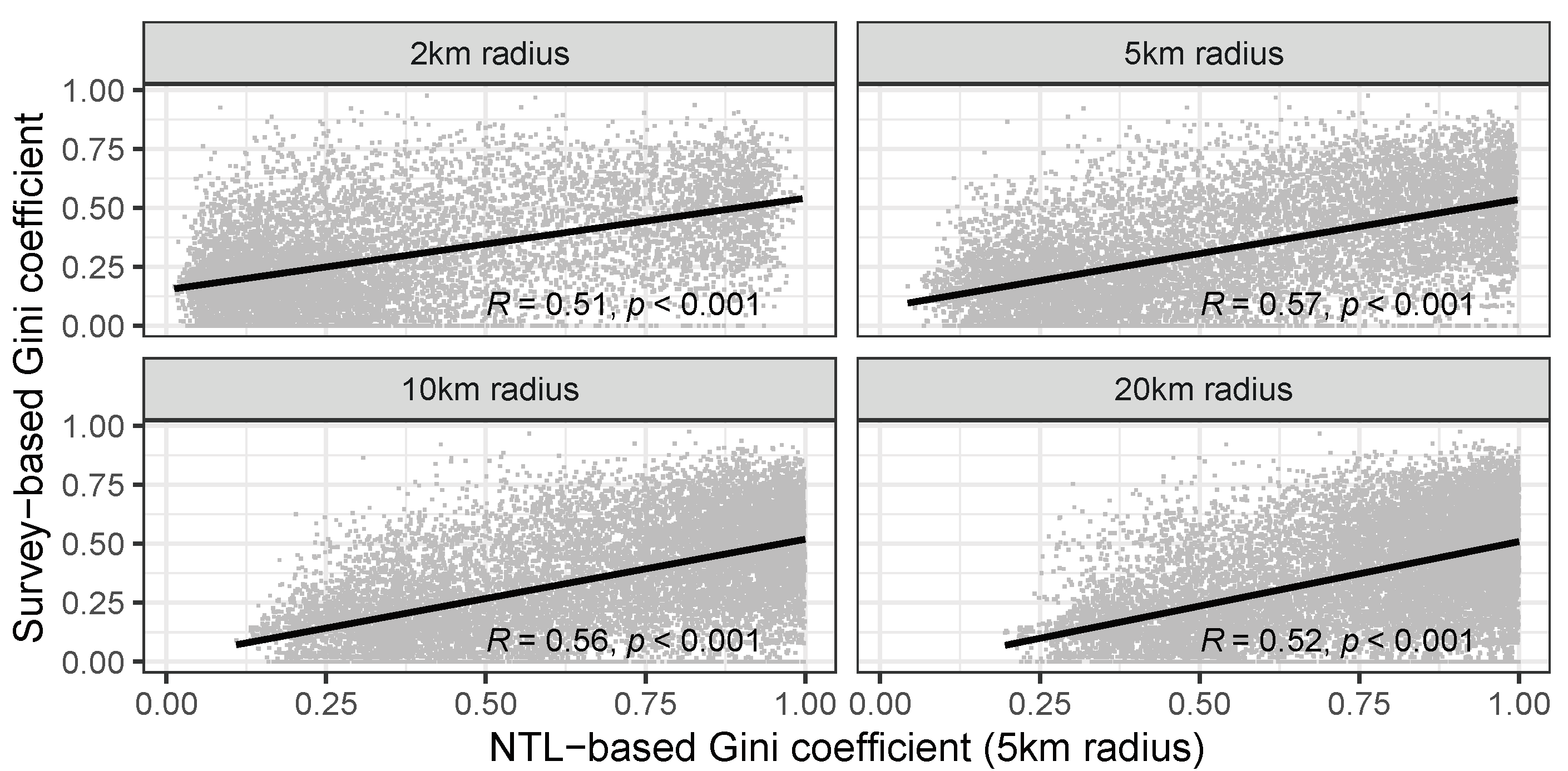In line with results by Weidmann and Schutte [6], we log-transform the nighttime light value before computing the inequality estimates. In our analysis below, we vary the buffer size from 2 km to 20 km, to find out what produces the most accurate estimates of local inequality. 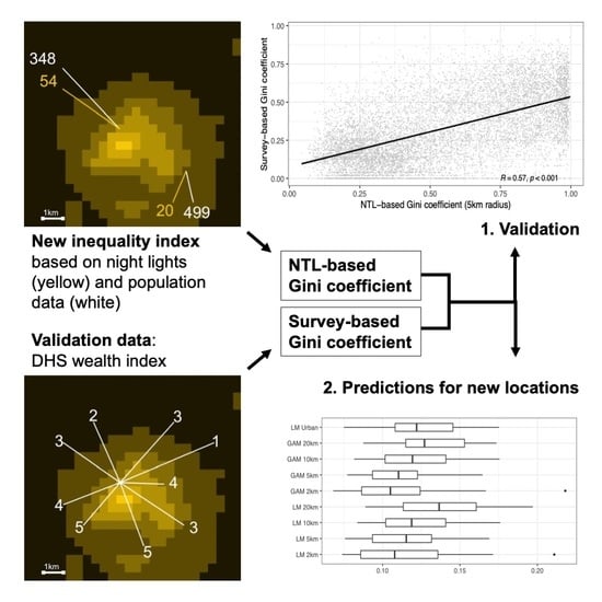Figure 1 (left panel) illustrates the data we use for this procedure. In principle, it is possible with this approach to compute local inequality estimates for any point on the globe. For our validation exercise below, we do this for the spatial locations where the survey was conducted, which allows us to compare survey-based inequality estimates to those calculated from the nighttime lights.

For our validation exercise, we require alternative estimates of local inequality. For countries where detailed official income or wealth statistics are available, these estimates can easily be computed (as for example in [33]). However, for many countries in particular in the Global South, these data cannot be used for research purposes, or are simply not collected regularly. This is why we rely on large cross-national survey data from the Demographic and Health Surveys (DHS) project (see https://dhsprogram.com, accessed on 30 July 2021). The DHS is a regular survey on living conditions and health-related data that is conducted across many countries. It uses the same survey instrument in all countries, which contains questions at the individual level but also the household level. Most importantly, the DHS also include an assessment of the household’s wealth by means of a wealth index. The wealth index is created from different questions answered by the enumerator (not the respondents) about the household’s assets. These answers are collapsed to the most important underlying dimension using factor analysis, and the factor scores are used to assign each household to its corresponding quintile in the distribution of scores in the country [34]. The household’s quintile (1–5) is the wealth index for this household. 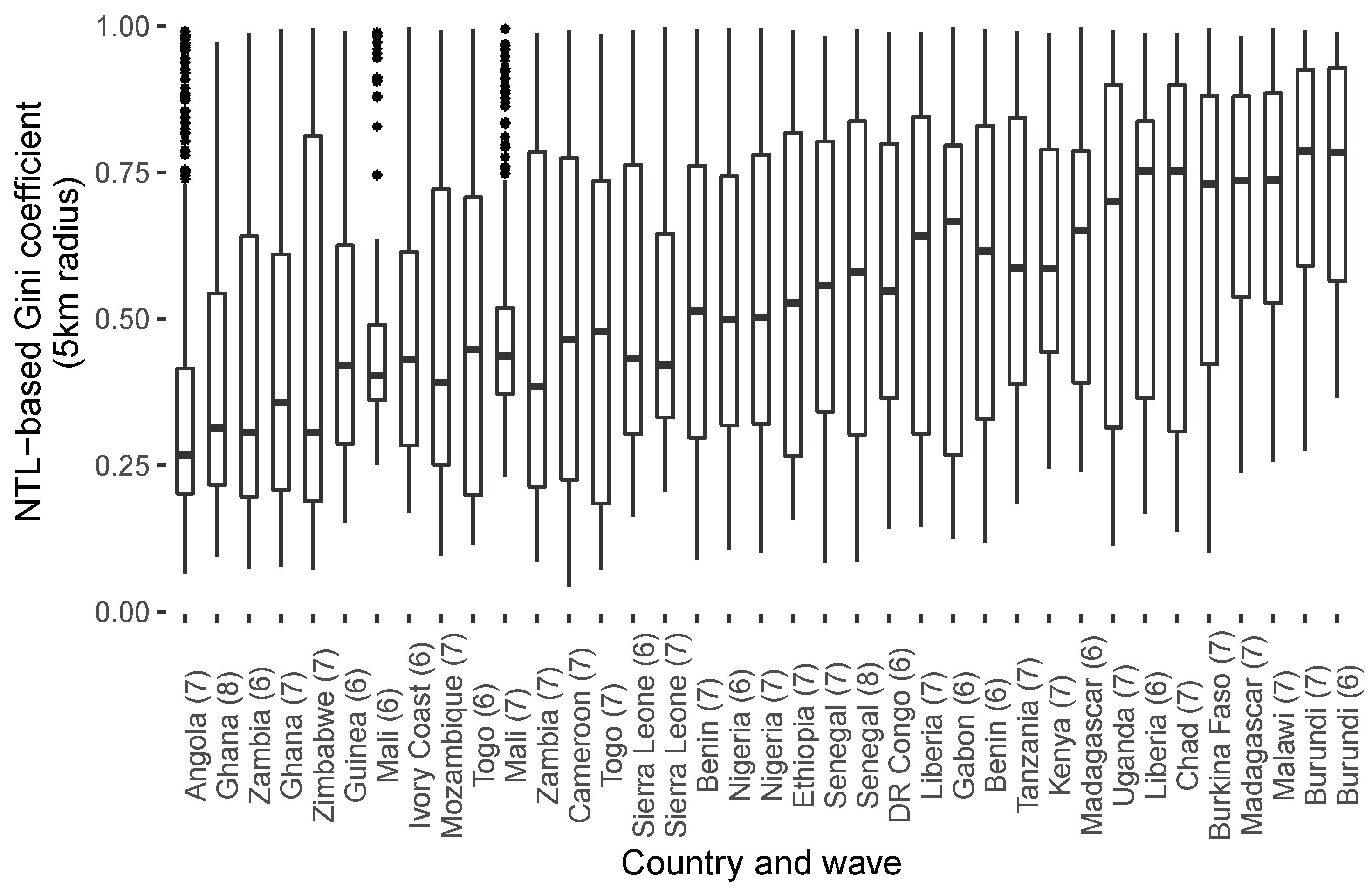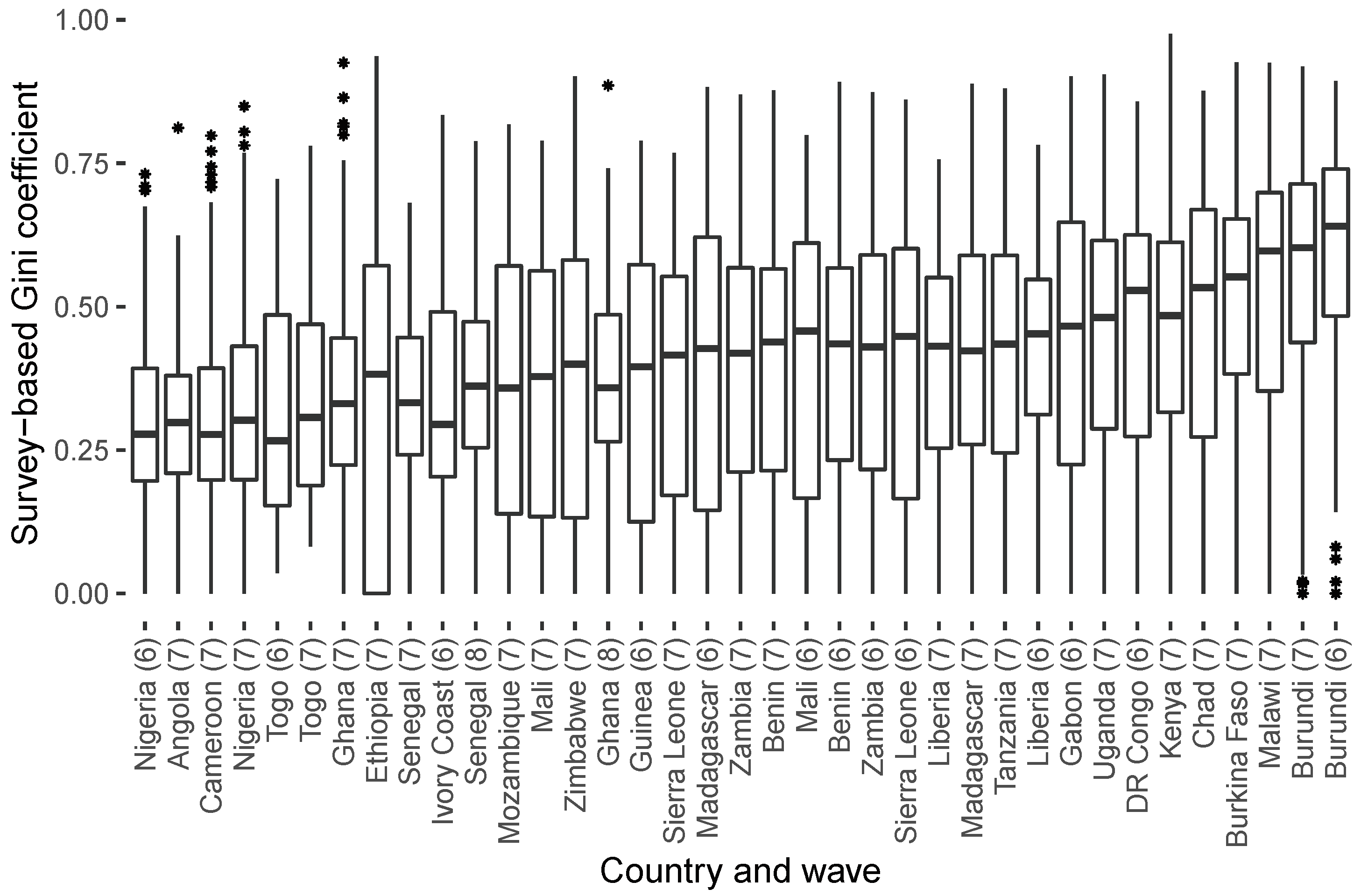Figure 1 (right panel) gives an example of the DHS data we use for the validation. The entire sample covers 26 countries from DHS survey waves 6, 7 and 8, with data collected in the years 2012–2019. Appendix A lists all the countries and survey waves included in the sample.

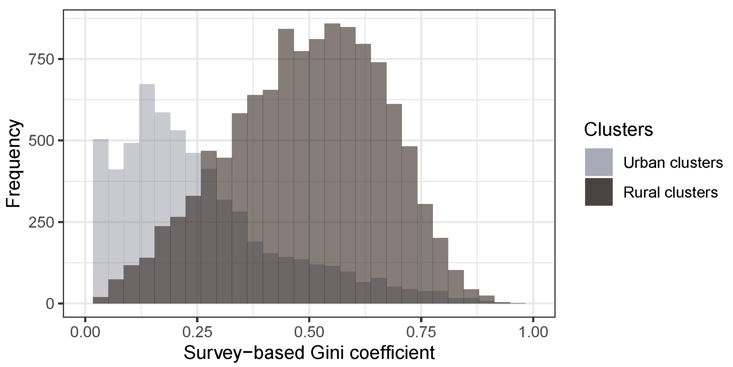
To link the survey results to our spatial index of local inequality, we also require geographic information about the location of households in the survey. These coordinates are not provided at the level of households, but at the level of survey clusters or primary sampling units (PSUs). 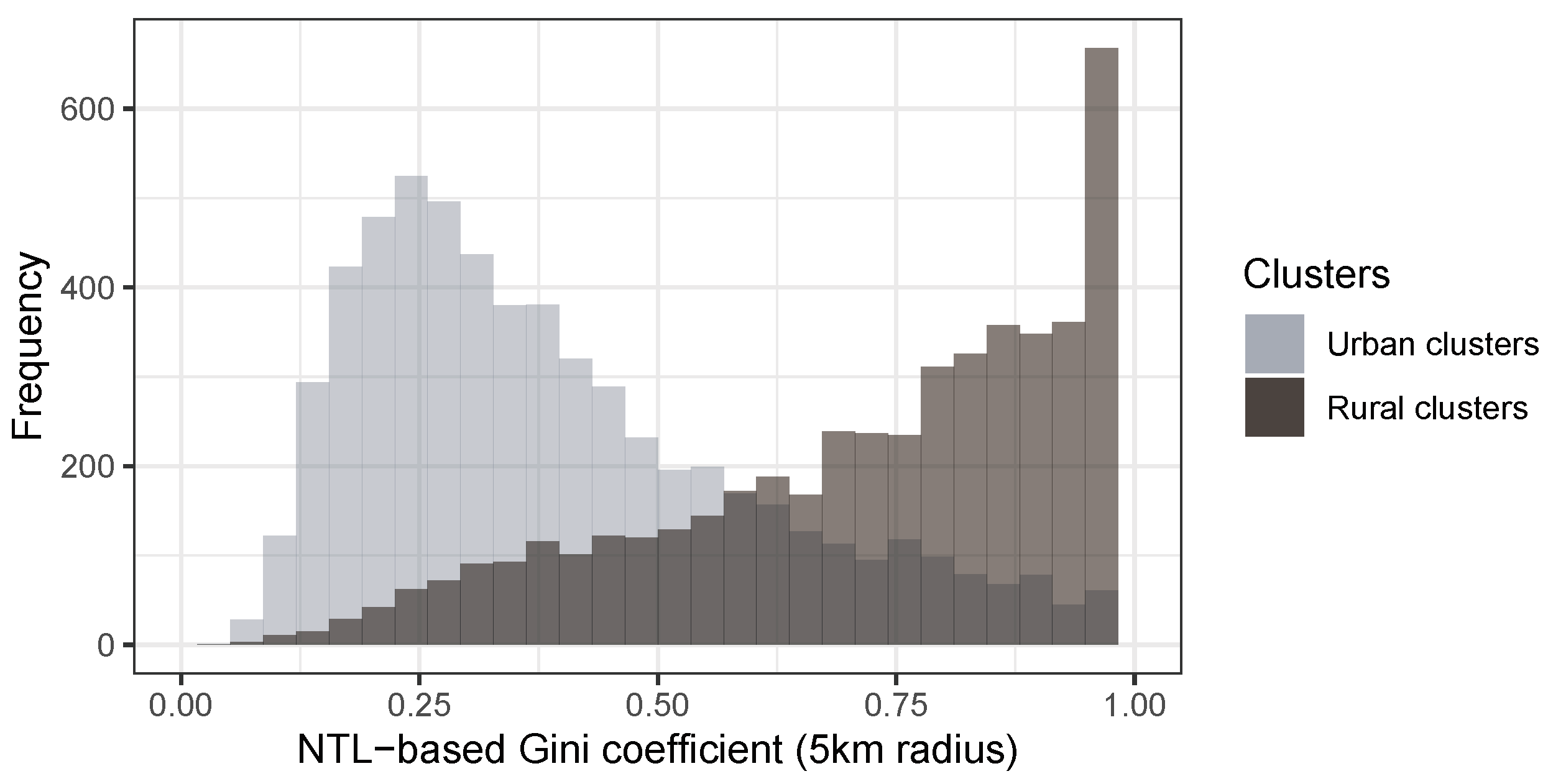In the DHS, a cluster is a group of about 25–30 households in close proximity to each other, which were selected according to the DHS’s sampling scheme [35]. The DHS categorize clusters into urban and rural ones. For each cluster, the DHS provide a point (longitude/latitude) location, which, however, is randomly distorted to preserve anonymity in the data. More precisely, an urban cluster’s location is randomly shifted within a radius of 2 km, while a rural location is assigned a random location with a radius of 5 km of its original location (10 km for a randomly chosen 1% of all rural clusters in a given country and survey wave). Therefore, the spatial reference for the survey cluster is approximate, and we construct the spatial buffers for the computation of our local inequality index such that it contains the original cluster location (with the exception of the randomly chosen 1% of the rural cluster with a spatial error of up to 10 km, which introduces measurement error in our analysis that we cannot prevent).

For our survey-based measure of local inequality, we compute the Gini inequality coefficient over the wealth index values of all households in a cluster. Since the input values have a limited range of 1–5, the upper bound of the Gini coefficients is less than 1 (the usual upper bound of the Gini index). To normalize the resulting coefficient values, we divide them by 0.382. The derivation for this value is presented in Appendix B.

3. Results

In this section, we first present the satellite-based and survey-derived estimates of local inequality separately, before turning to a comparison of the two.

3.1. Estimates of Local Inequality from Nighttime Lights Data

As stated above, we compute spatial estimates of local inequality for all survey cluster locations in our sample, so that we can later compare them to the survey-derived inequality scores. These computations use NTL data for the same year in which the cluster was included in the survey (see below). In Figure 2, we show the overall distribution of our spatial estimates, computed with a buffer radius of 5 km. The distribution is bimodal, which is an aggregate result of the different distributions of urban and rural clusters: While urban clusters tend to have low values of inequality (most of them located around 0.20), the opposite is true for rural clusters. Here, the majority of the cases has Gini values of 0.5 and above. This could partly reflect more segregated residential patterns in cities, where neighborhoods tend to be inhabited by similarly poor or rich households. This could be different in rural areas, where rich and poor households can be located close to each other, thus resulting in a high level of local inequality.

At the same time, this pattern can also indicate potential limitations of our satellite-based measurement method. In urban areas, a small buffer radius (2 km or 5 km) will include many cells with similar levels of illumination and similar population counts, thus leading to low levels of the NTL-based inequality indicator. A plot of the inequality scores for different buffer sizes (see Figure 3 partly confirms this: as the buffer size increases, cells within the buffers become more diverse as regards their illumination and population values, and inequality scores increase as a result. Our validation exercise later will have to test how buffer size affects the correlation between NTL-based and survey-based inequality scores, and which of them results in the best fit.

We also show the distribution of nightlight-based inequality scores separately for each country in Figure 4. The results show that the distribution of NTL-based local inequality values differs by country. Our validation exercise will have to test whether these patterns reflect actual differences in local inequality.

3.2. Estimates of Local Inequality from the DHS

What is the level of local inequality according to the survey data from the DHS? In Figure 5, we plot the overall distribution of the survey-based inequality scores, distinguishing again between urban and rural clusters. Again, we observe a similar distribution as for the NTL-based estimates above, with urban clusters on average exhibiting lower levels of local inequality, while rural clusters have high Gini values. This is somewhat reassuring, since it shows that the patterns we found for the nightlight-based indicator above are not entirely driven by the measurement method.

We again plot the indicator distribution separately for each country (see Figure 6). In contrast to the pronounced differences between countries for the NTL-based indicator, we see considerably less variation across countries here, with most distributions centered in the range 0.25–0.5.

3.3. Validation

In this section, we compare the local inequality estimates obtained from the surveys to those computed from the nighttime light data. As explained above, for each survey cluster and the associated level of (survey-based) local inequality, we compute a nightlight-based estimate for the same year in which the survey was conducted. In Figure 7, we show simple scatterplots of the two indicators, as well as a line indicating the linear fit. Overall, the plot shows a positive and significant correlation between the two indicators. In other words, our nightlight-based indicator is able to pick up some of the variation in local inequality we see in the surveys. Still, the large point clouds also indicate that there is considerable error where the two indicators disagree.

To test how buffer size affects the fit between the nightlight-based and the survey-derived indicator, we plot the full distribution of clusters for different buffer sizes in Figure 8. Here, we see that neither small nor large buffer sizes maximize the fit between the two indicators. Rather, a buffer size of 5 km seems to give the best results over the entire sample.

Can we also observe different patterns for the different countries in our analysis? Following our approach above, we plot the two indicators separately for each country in Figure 9. In all countries except one (Ghana), the correlation between them is positive, which is encouraging. In some countries, we observe high levels of agreement (as for example, Burkina Faso, Uganda or Zambia), while in a few others, our satellite-based measurement method does not seem to work well. In Gabon and Ghana, for example, correlations between the indicators remain low.

Our bivariate comparison of survey-based and NTL-based indicators cannot control for other factors that could potentially affect the positive correlation we find between the nightlight-based and the survey-based indicator. For that reason, we run multivariate regression models for each buffer size (2 km, 5 km, 10 km and 20 km), with the survey-derived Gini coefficient as the outcome. Our main predictor is the inequality index computed from the satellite data. We include a number of control variables. First, we include a dummy variable for urban clusters, to remove variation in the outcome that is driven by the difference between urban and rural locations (see the discussion above). We also control for demographic factors such as the average size of the household, as well as the number of households included in the cluster. To make sure that the results are driven by inequality in the nightlight emissions and not the overall level of emissions or the size of the buffer, we also control for the sum of the nighttime light emissions in a buffer, and the total population as well as the number of cells in the buffer. The results of the regression models are shown in

Table 1. OLS regression results. Dependent variable: survey-based Gini coefficient. Standard errors clustered by country and survey wave.

	Survey-Based Inequality Index
	Radius
	2 km	5 km	10 km	20 km
	(1)	(2)	(3)	(4)
Intercept	0.638 ***	0.626 ***	0.507 ***	0.327 ***
	(0.027)	(0.028)	(0.029)	(0.030)
NTL-based Gini	0.098 ***	0.165 ***	0.211 ***	0.265 ***
	(0.009)	(0.009)	(0.009)	(0.009)
Urban	−0.088 ***	−0.116 ***	−0.152 ***	−0.177 ***
	(0.005)	(0.004)	(0.004)	(0.004)
Household size (mean)	0.002 *	−0.001	−0.002 *	−0.001
	(0.001)	(0.001)	(0.001)	(0.001)
Number of households	0.0003	−0.0005	−0.001 ***	−0.002 ***
	(0.0003)	(0.0003)	(0.0003)	(0.0003)
Total NTL emissions (log)	−0.003 ***	−0.001 ***	−0.0002 ***	−0.0001 ***
	(0.0004)	(0.0001)	(0.00002)	(0.00001)
Total population (log)	−0.042 ***	−0.031 ***	−0.016 ***	−0.003
	(0.002)	(0.002)	(0.002)	(0.002)
Number of cells	0.005 ***	0.002 *	0.001	0.001
	(0.001)	(0.001)	(0.001)	(0.001)
Observations	9343	11,029	12,946	15,211
R${}^2$	0.423	0.437	0.421	0.398
Adjusted R${}^2$	0.423	0.437	0.421	0.398
Residual Std. Error	0.158 (df = 9335)	0.163 (df = 11,021)	0.168 (df = 12,938)	0.172 (df = 15,203)

Note: * p < 0.1; *** p < 0.01.

. We provide additional results with country/wave fixed effects in

Table 2. OLS regression results with country/wave fixed effects. Dependent variable: survey-based Gini coefficient. Standard errors clustered by country/survey wave.

	Survey-Based Inequality Index
	Radius
	2 km	5 km	10 km	20 km
	(1)	(2)	(3)	(4)
Intercept	0.218 ***	0.164 ***	0.042	−0.115 ***
	(0.034)	(0.035)	(0.035)	(0.037)
NTL-based Gini	0.105 ***	0.171 ***	0.207 ***	0.257 ***
	(0.009)	(0.009)	(0.009)	(0.011)
Urban	−0.079 ***	−0.103 ***	−0.137 ***	−0.162 ***
	(0.005)	(0.004)	(0.004)	(0.004)
Household size (mean)	0.015 ***	0.011 ***	0.010 ***	0.010 ***
	(0.001)	(0.001)	(0.001)	(0.001)
Number of households	0.007 ***	0.008 ***	0.008 ***	0.008 ***
	(0.001)	(0.001)	(0.001)	(0.001)
Total NTL emissions (log)	−0.008 ***	−0.001 ***	−0.0003 ***	−0.0001 ***
	(0.0004)	(0.0001)	(0.00002)	(0.00001)
Total population (log)	−0.018 ***	−0.014 ***	−0.005 ***	0.004 *
	(0.002)	(0.002)	(0.002)	(0.002)
Number of cells	0.007 ***	0.001 ***	0.0002 ***	0.00005 ***
	(0.001)	(0.0002)	(0.00003)	(0.00001)
Fixed effects (country/wave)	Yes	Yes	Yes	Yes
Observations	9343	11,029	12,946	15,211
R${}^2$	0.539	0.532	0.508	0.470
Adjusted R${}^2$	0.537	0.530	0.507	0.469
Residual Std. Error	0.142 (df = 9299)	0.149 (df = 10,985)	0.155 (df = 12,902)	0.161 (df = 15,167)

Note: * p < 0.1; *** p < 0.01.

, to take into account systematic differences between countries and survey waves.

The regression results confirm that our NTL-based indicator remains a strong predictor of actual local inequality. We see that in both types of regression and for all four buffer sizes, the coefficient of this variable remains positive and highly significant. This results holds in the presence of several control variables. For example, the “urban” dummy nets out the difference between urban and rural clusters we have seen above, with urban clusters having lower levels of inequality. Furthermore, the effect of the NTL-based indicator remains when we control for the overall level of night light emissions and the total population, which are additional controls that go beyond the simple urban/rural distinction and provide additional support for the impact of our NTL-based indicator. In Appendix C, we provide additional results that limit the sample to clusters with at least 30 households, since we may be concerned that survey-based local inequality may be measured with considerable error if we have fewer observations in a cluster. Furthermore, we repeat the analysis without log-transforming the NTL. The substantive results from our main analysis remain unchanged. In short, these results show that our indicator can capture local inequality well and that the relationship we see is not due to some a spurious correlation with other characteristics of the survey clusters and their spatial features.

3.4. Predicting Local Inequality from Nighttime Lights Data

Our above analyses show that the nightlight-based indicator picks up variation in local inequality, even when we control for a number of factors that could be driving this result. In a final analysis, we move from correlation analysis to prediction. We analyze a situation where a researcher requires estimates of local inequality, and uses simple machine learning models to predict these values based on our NTL indicator with a model fitted on available data from other locations. Specifically, we study two scenarios. In the first one, we use data from a given country to fit a prediction model, and then predict local inequality for a new location. In the second and more difficult scenario, we predict local inequality for a new country with a prediction model fitted on data from other countries. For both scenarios, our aim is to gauge the average prediction error that the researcher would have to incur when relying solely on our NTL indicator.

In both scenarios, we use very simple prediction models. Our first model is an OLS regression model similar to the one we have used above, but with only one predictor: the nightlight-based estimate of local inequality. The second model is a generalized additive model (GAM) using quadratically penalized likelihood, fitted using the gam function from R’s mgcv package (see [36]), while more complex machine learning models could be applied, we do not expect significant performance gains due to the simple setup of the prediction exercise with a single predictor only. We evaluate all our models out-of-sample. In the first prediction scenario, this means that we keep a single cluster in a country as a hold-out, fit the model on the remaining clusters from that country, and then predict the level of local inequality for the cluster that was set aside. In Figure 10, we show the distribution of the absolute prediction errors across the 37 surveys in our sample, for satellite-based inequality indicators with different buffer sizes (2 km, 5 km, 10 km and 20 km) and the two different prediction models (LM and GAM). For comparison, we add an additional linear model that only contains a binary predictor for urban vs. rural locations. The tabular presentation of the results is provided in Appendix D.

The plot shows that prediction of local inequality for new locations using our spatial indicator works well. Using small buffer sizes (2 km), we miss the level of local inequality as given by the survey data only by around 0.11 on average, and 75% of the cases have an error of less than 0.125 (for the GAM). The GAM performs slightly better than the LM, but the differences are small.

In our second prediction scenario, we predict local inequality in a new country that was not used in training the model. We again use leave-one-out cross-validation, where we fit the model on all our data except one country, and then predict the values for that country. In Figure 11, we show again the distribution of absolute prediction errors for this exercise.

Figure 11 shows that as expected, prediction errors are higher as compared to the first scenario. This is not surprising, since in the second scenario, the model is not able to capture a possible country-specific relationship between the satellite-based estimates and the survey-based inequality indicator. Still, prediction errors are again of limited magnitude even in the more difficult scenario. However, unlike in the first prediction task, we see that our NTL-based indicator improves predictive performance only marginally as compared to the simple model using only the urban/rural dummy (“LM Urban”) in Figure 11. In particular, the 5 km buffers seem to work best. Together, these results show that we can use our NTL-based indicator in a simple machine learning model to obtain local inequality estimates for new locations in a given country, but in particular for cases where we do have some training/calibration data available for the same country.

4. Discussion

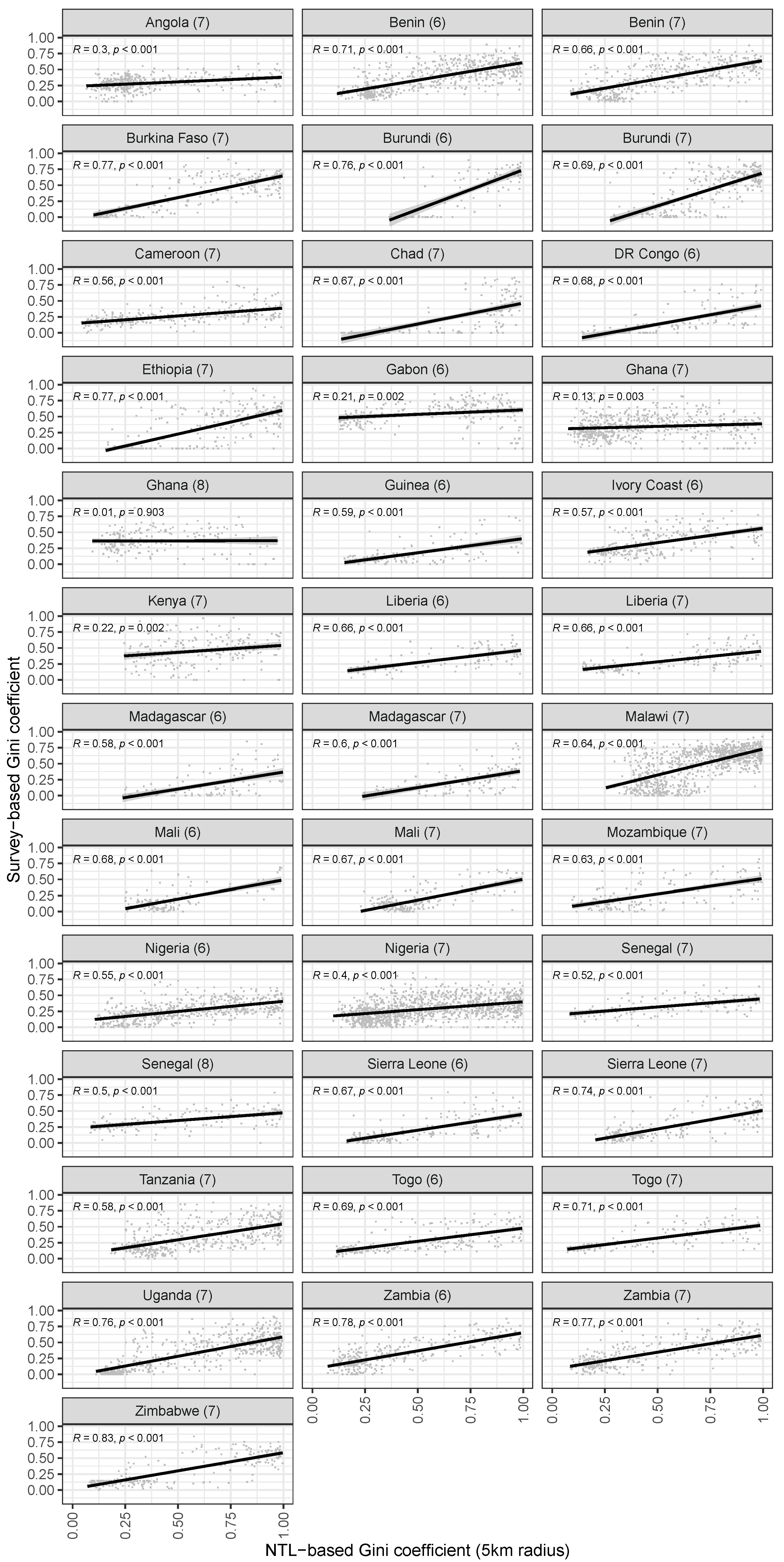
In this article, we have introduced an indicator for local inequality derived from high-resolution night lights data. In addition to the night lights raster data, the computation of this indicator requires only a fine-grained population grid, both of which are freely available. We combine these two data sources to obtain per capita emissions values at the grid cell level, which we use to compute a Gini index of inequality for spatial buffers of a given size. We present two main analyses. In a first validation exercise, we compare the NTL-based indicator to estimates of local inequality derived from survey data. The correlations are positive and significant in almost all countries in our sample, although not surprisingly, the indicator cannot fully capture local inequality as measured by the surveys. This is to be expected: while survey estimates of wealth take into account a variety of household assets, only some of them are related to electricity consumption and are therefore possibly reflected in nightlight emissions. Furthermore, in particular in urban areas, night light emissions are less likely to be attributable to individual households, and rather reflect public infrastructure. This will also reduce the correlation between NTL emissions and individual wealth.

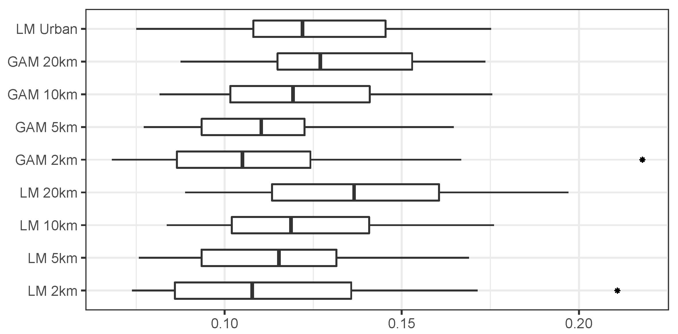
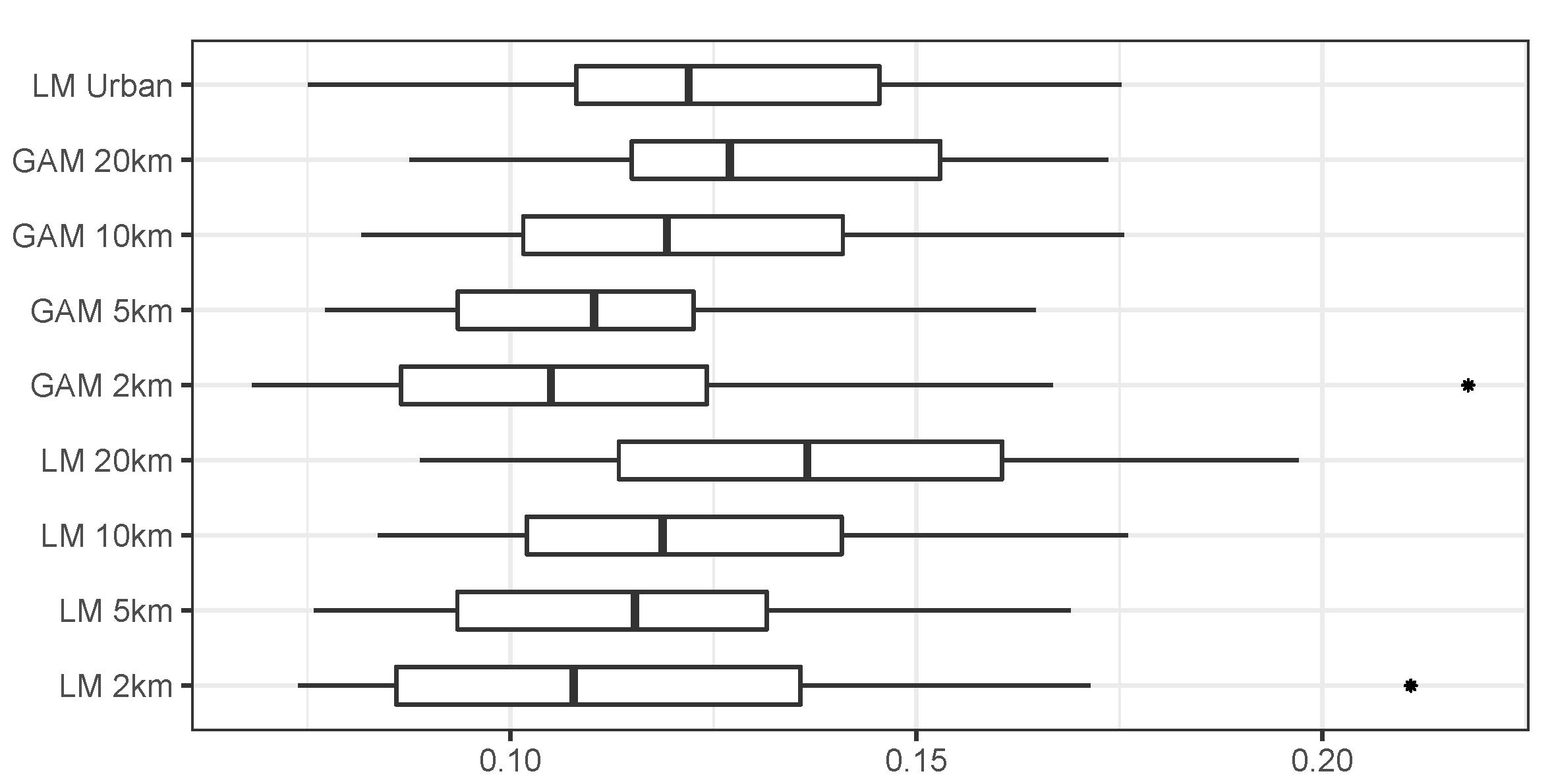
To address the question of whether it is possible to our indicator for locations where no other data are available, we provide a second type of analysis. Here, we generate estimates of local inequality with simple prediction models, and compare these predicted values to the ones measured with the survey data. This analysis shows that prediction errors are generally low. When we predict Gini coefficients of local inequality with our NTL-based indicator, the best predictions have an average error around 0.05 on the 0–1 scale. This is a good result, given that it is derived exclusively from simple spatial datasets (night light emissions and population rasters). Overall, this shows that our approach can be used to generate new estimates of local inequality for locations for which no other data exists.

While our results show that night lights emission can pick up local inequality to a certain extent, they are necessarily weaker as compared to other approaches combining multiple sources of data. For example, Chi et al. [37] introduce micro-level estimates of wealth that are computed using a variety of input data, including telecommunication coverage maps as well as Facebook connectivity data. This leads to better wealth estimates, which could also be used to estimate local inequality. At the same time, however, the use of proprietary data makes this approach impossible to use for many researchers without access to these data. Furthermore, the coverage of these data may be limited to particular countries, which restricts their applicability to country-specific studies. Our approach, in contrast, uses only publicly available data, is fully replicable using open-source software (PostGIS), and can be used for comparative, cross-national work in the social sciences.

Due to its ability to pick up variation in local inequality and its exclusive reliance on publicly available data, our index enables future research in many different fields. In political science, for example, it helps to better understand how local inequality in an individual’s immediate context affects political preferences and behavior. Sociologists can use these data to study the effect of local inequality on residential choice or personal relationships, and development economists can use it to identify areas in need of particular support.

While the results presented in our article are encouraging, there are several drawbacks associated with the NTL-based estimation of inequality. Due to its reliance on variation in night light emissions, this approach can only work in world regions where no saturation has been reached. For example, in most countries of the Global North, nightly illumination of streets is commonplace, which reduces variation in night light emissions and their correlation with socio-economic variables [38]. Consequently, we expect our approach to be less applicable to these countries. Furthermore, there are limitations as regards the temporal variation the indicator is able to pick up. Night light emissions change slowly, which is why our indicator will remain relatively stable even in cases of large population shifts, for example due to refugee movements. When relying on night lights as a proxy for wealth or inequality, researchers should be aware of these limitations and carefully consider whether this data source is suitable for their project.

References

1. Cederman, L.E.; Gleditsch, K.S. Introduction to Special Issue on ’Disaggregating Civil War’. J. Confl. Resolut. 2009, 53, 487–495. [Google Scholar] [CrossRef] [Green Version]
2. Elvidge, C.D.; Baugh, K.E.; Kihn, E.A.; Kroehl, H.W.; Davis, E.R.; Davis, C.W. Relation between Satellite Observed Visible-Near Infrared Emissions, Population, Economic Activity and Electric Power Consumption. Int. J. Remote Sens. 1997, 18, 1373–1379. [Google Scholar] [CrossRef]
3. Elvidge, C.D.; Sutton, P.C.; Ghosh, T.; Tuttle, B.T.; Baugh, K.E.; Bhaduri, B.; Bright, E. A Global Poverty Map Derived from Satellite Data. Comput. Geosci. 2009, 35, 1652–1660. [Google Scholar] [CrossRef]
4. Ghosh, T.; Powell, R.L.; Elvidge, C.D.; Baugh, K.E.; Sutton, P.C.; Anderson, S. Shedding Light on the Global Distribution of Economic Activity. Open Geogr. J. 2010, 3, 148–161. [Google Scholar]
5. Elvidge, C.D.; Baugh, K.E.; Anderson, S.J.; Sutton, P.C.; Ghosh, T. The Night Light Development Index (NLDI): A Spatially Explicit Measure of Human Development from Satellite Data. Soc. Geogr. 2012, 7, 23–35. [Google Scholar] [CrossRef]
6. Weidmann, N.B.; Schutte, S. Using Night Light Emissions for the Prediction of Local Wealth. J. Peace Res. 2017, 54, 125–140. [Google Scholar] [CrossRef]
7. Zhou, Y.; Ma, T.; Zhou, C.; Xu, T. Nighttime Light Derived Assessment of Regional Inequality of Socioeconomic Development in China. Remote Sens. 2015, 7, 1242–1262. [Google Scholar] [CrossRef] [Green Version]
8. Bruederle, A.; Hodler, R. Nighttime Lights as a Proxy for Human Development at the Local Level. PLoS ONE 2018, 13, e0202231. [Google Scholar] [CrossRef] [Green Version]
9. Wu, R.; Yang, D.; Dong, J.; Zhang, L.; Xia, F. Regional Inequality in China Based on NPP-VIIRS Night-Time Light Imagery. Remote Sens. 2018, 10, 240. [Google Scholar] [CrossRef] [Green Version]
10. Ivan, K.; Holobâcă, I.H.; Benedek, J.; Török, I. Potential of Night-Time Lights to Measure Regional Inequality. Remote Sens. 2020, 12, 33. [Google Scholar] [CrossRef] [Green Version]
11. Ivan, K.; Holobâcă, I.H.; Benedek, J.; Török, I. VIIRS Nighttime Light Data for Income Estimation at Local Level. Remote Sens. 2020, 12, 2950. [Google Scholar] [CrossRef]
12. Piketty, T. Capital in the 21st Century; Harvard University Press: Cambridge, MA, USA, 2014. [Google Scholar]
13. Cederman, L.E.; Weidmann, N.B.; Gleditsch, K.S. Horizontal Inequalities and Ethno-nationalist Civil War: A Global Comparison. Am. Political Sci. Rev. 2011, 105, 478–495. [Google Scholar] [CrossRef] [Green Version]
14. Cederman, L.E.; Weidmann, N.B.; Bormann, N.C. Triangulating Horizontal Inequality: Toward Improved Conflict Analysis. J. Peace Res. 2015, 52, 806–821. [Google Scholar] [CrossRef] [Green Version]
15. Alesina, A.; Michalopoulos, S.; Papaioannou, E. Ethnic Inequality. J. Political Econ. 2016, 124, 428–488. [Google Scholar] [CrossRef] [Green Version]
16. Bormann, N.C.; Pengl, Y.I.; Cederman, L.E.; Weidmann, N.B. Globalization, Institutions, and Ethnic Inequality. Int. Organ. 2021, 75, 665–697. [Google Scholar] [CrossRef]
17. Kuhn, P.; Weidmann, N.B. Unequal We Fight: Between- and Within-Group Inequality and Ethnic Civil War. Political Sci. Res. Methods 2015, 3, 543–568. [Google Scholar] [CrossRef] [Green Version]
18. Neman, T.S. Does Your Neighborhood’s Income Distribution Matter? A Multi-scale Study of Financial Well-Being in the U.S. Soc. Indic. Res. 2020, 152, 951–970. [Google Scholar] [CrossRef]
19. Newman, B.J. Breaking the Glass Ceiling: Local Gender-Based Earnings Inequality and Women’s Belief in the American Dream. Am. J. Political Sci. 2016, 60, 1006–1025. [Google Scholar] [CrossRef]
20. Newman, B.J.; Hayes, T.J. Durable Democracy? Economic Inequality and Democratic Accountability in the New Gilded Age. Political Behav. 2019, 41, 5–30. [Google Scholar] [CrossRef]
21. Newman, B.J.; Johnston, C.D.; Lown, P.L. False Consciousness or Class Awareness? Local Income Inequality, Personal Economic Position, and Belief in American Meritocracy. Am. J. Political Sci. 2015, 59, 326–340. [Google Scholar] [CrossRef]
22. Newman, B.J.; Shah, S.; Lauterbach, E. Who Sees an Hourglass? Assessing Citizens’ Perception of Local Economic Inequality. Res. Politics 2018, 5, 2053168018793974. [Google Scholar] [CrossRef] [Green Version]
23. Sands, M.L.; de Kadt, D. Local Exposure to Inequality Raises Support of People of Low Wealth for Taxing the Wealthy. Nature 2020, 586, 257–261. [Google Scholar] [CrossRef]
24. Larsen, M.V.; Hjorth, F.; Dinesen, P.T.; Sønderskov, K.M. When Do Citizens Respond Politically to the Local Economy? Evidence from Registry Data on Local Housing Markets. Am. Political Sci. Rev. 2019, 113, 499–516. [Google Scholar] [CrossRef] [Green Version]
25. Hu, Y.; Peng, J.; Liu, Y.; Du, Y.; Li, H.; Wu, J. Mapping Development Pattern in Beijing-Tianjin-Hebei Urban Agglomeration Using DMSP/OLS Nighttime Light Data. Remote Sens. 2017, 9, 760. [Google Scholar] [CrossRef] [Green Version]
26. Mukhopadhyay, A.; Urzainqui, D.G.; The Dynamics of Spatial and Local Inequalities in India. UN-WIDER Working Paper. 2019. Available online: https://www.wider.unu.edu/publication/dynamics-spatial-and-local-inequalities-india (accessed on 30 July 2021).
27. Elvidge, C.D.; Zhizhin, M.; Ghosh, T.; Hsu, F.C.; Taneja, J. Annual Time Series of Global VIIRS Nighttime Lights Derived from Monthly Averages: 2012 to 2019. Remote Sens. 2021, 13, 922. [Google Scholar] [CrossRef]
28. Elvidge, C.D.; Baugh, K.E.; Zhizhin, M.; Hsu, F.C. Why VIIRS Data are Superior to DMSP for Mapping Nighttime Lights. Proc.-Asia-Pac. Adv. Netw. 2013, 35, 62. [Google Scholar] [CrossRef] [Green Version]
29. Chen, X.; Nordhaus, W. A Test of the New VIIRS Lights Data Set: Population and Economic Output in Africa. Remote Sens. 2015, 7, 4937–4947. [Google Scholar] [CrossRef] [Green Version]
30. Gibson, J.; Olivia, S.; Boe-Gibson, G. Night Lights in Economics: Sources and Uses. J. Econ. Surv. 2020, 34, 955–980. [Google Scholar] [CrossRef]
31. Tatem, A.J. WorldPop, Open data for Spatial Demography. Sci. Data 2017, 4, 170004. [Google Scholar] [CrossRef]
32. Lloyd, C.T.; Chamberlain, H.; Kerr, D.; Yetman, G.; Pistolesi, L.; Stevens, F.R.; Gaughan, A.E.; Nieves, J.J.; Hornby, G.; MacManus, K.; et al. Global Spatio-temporally Harmonised Datasets for Producing High-resolution Gridded Population Distribution Datasets. Big Earth Data 2019, 3, 108–139. [Google Scholar] [CrossRef] [Green Version]
33. Sønderskov, K.M.; Dinesen, P.T.; Finkel, S.E.; Hansen, K.M. Crime Victimization Increases Turnout: Evidence from Individual-level Administrative Panel Data. Br. J. Political Sci. 2020. [Google Scholar] [CrossRef]
34. Rutstein, S.O.; Johnson, K.; The DHS Wealth Index. DHS Comparative Reports No. 6. 2004. Available online: http://dhsprogram.com/pubs/pdf/CR6/CR6.pdf (accessed on 30 July 2021).
35. ICF International. Demographic and Health Survey Sampling and Household Listing Manual. Technical Documentation. 2012. Available online: https://dhsprogram.com/pubs/pdf/DHSM4/DHS6_Sampling_Manual_Sept2012_DHSM4.pdf (accessed on 30 July 2021).
36. Wood, S.N. Generalized Additive Models: An Introduction with R; CRC Press: Boca Raton, FL, USA, 2017. [Google Scholar]
37. Chi, G.; Fang, H.; Chatterjee, S.; Blumenstock, J.E. Micro-Estimates of Wealth for all Low- and Middle-Income Countries. CEGA Working Paper Series No. WPS-165. 2021. Available online: https://escholarship.org/uc/item/3fv3h12q (accessed on 30 July 2021).
38. Mellander, C.; Lobo, J.; Stolarick, K.; Matheson, Z. Night-time Light Data: A Good Proxy Measure for Economic Activity? PLoS ONE 2015, 10, e0139779. [Google Scholar] [CrossRef] [PubMed] [Green Version]
Figure 1. Satellite imagery of nighttime light emissions in raster format for the town Kansanshi in Zambia. (Left panel): The computation of the local Gini coefficient requires log-transformed nighttime light emissions at the level of cells (in yellow) and population estimates (in white). (Right panel): The DHS Wealth Index values of the households in the survey cluster at that location. All values are hypothetical and only displayed for illustration purposes.
Remotesensing 13 04624 g001
Figure 2. Histogram of the overall distribution of nightlight-based Gini-coefficients, computed with a buffer radius of five kilometers. The light-grey histogram shows the distribution of urban clusters, the distribution of rural clusters is shown in dark-grey.
Remotesensing 13 04624 g002
Figure 3. Histogram of the overall distribution of nightlight-based Gini-coefficients for different buffer sizes.
Remotesensing 13 04624 g003
Figure 4. Boxplot of the NTL-based Gini-coefficients for a buffer radius of 5 km for individual countries. The lower and upper hinges correspond to the 25th and 75th percentiles, and the centerline indicates the 50th percentile.
Remotesensing 13 04624 g004
Figure 5. Histogram of the overall distribution of survey-based Gini-coefficients. Distribution of urban clusters in light-grey, the dark-grey histogram shows the distribution of rural clusters.
Remotesensing 13 04624 g005
Figure 6. Boxplot of the distribution of survey-based Gini coefficients for the individual countries. The number indicates the survey wave.
Remotesensing 13 04624 g006
Figure 7. Scatterplot of NTL-based Gini coefficients (computed with a buffer size of five kilometers) and survey-based Gini coefficients, separately for urban and rural clusters.
Remotesensing 13 04624 g007
Figure 8. Scatterplot of NTL-based and survey-based Gini coefficients, for different buffer sizes.
Remotesensing 13 04624 g008
Figure 9. Scatterplot of nighttime light-based Gini coefficients (with a buffer size of five kilometers) and survey-based Gini coefficients, by country and survey wave.
Remotesensing 13 04624 g009
Figure 10. Predicting wealth from nighttime light emissions, within-country. The figure shows the median (black lines), the 25th and 75th percentile (hinges) and the full ranges of the mean absolute prediction errors across the 37 surveys in our sample. Lower values indicate better performance.
Remotesensing 13 04624 g010
Figure 11. Predicting wealth from nighttime light emissions, across countries. As above, the figure shows the distribution of the mean absolute prediction errors across the 37 surveys in our sample, with lower values indicating better performance.
Remotesensing 13 04624 g011