Abstract
Aerosol optical depth is an important indicator of aerosol particle properties and their associated radiative impacts. AOD determination is very important to achieve relevant climate modelling. Most remote sensing techniques to retrieve aerosol optical depth are applicable to daytime given the high level of light available. The night represents half of the time but in such conditions only a few remote sensing methods are available. Among these approaches, the most reliable are moon photometers and star photometers. In this paper, we attempt to fill gaps in the aerosol detection performed with the aforementioned techniques using night sky brightness measurements during moonless nights with the novel CoSQM, a portable, low-cost and open-source multispectral photometer. In this paper, we present an innovative method for estimating the aerosol optical depth using an empirical relationship between the zenith night sky brightness measured at night with the CoSQM and the aerosol optical depth retrieved during daytime from the AErosol Robotic NETwork. Although the proposed method does not measure the AOD directly, an empirical relationship with the CE318-T is shown to give good results at the location of Santa Cruz de Tenerife. Such a method is especially suited to light-polluted regions with light pollution sources located within a few kilometres of the observation site. A coherent day-to-night aerosol optical depth and Ångström Exponent evolution in a set of 354 days and nights from August 2019 to February 2021 was verified at the location of Santa Cruz de Tenerife on the island of Tenerife, Spain. The preliminary uncertainty of this technique was evaluated using the variance under stable day-to-night conditions, set at 0.02 for aerosol optical depth and 0.75 for the Ångström Exponent. These results indicate the set of CoSQM and the proposed methodology appear to be a promising tool, adding new information on the optical properties of aerosols at night, which could be of key importance in improving climate predictions.
1. Introduction
The aerosol optical depth (AOD), which characterizes the total aerosol optical extinction at a given wavelength, is a key parameter in the monitoring of aerosol optical properties. AOD is sensitive to aerosol microphysical characteristics (in particular to the vertically integrated number density and to the particulate size distribution). The Ångström exponent (AE) of aerosols is related to the particles’ size distribution. In the case of hygroscopic aerosols such as sea salt or sulfate, these parameters are in turn sensitive to local relative humidity.
Many techniques have been developed in order to monitor the spatiotemporal variability of the AOD. A well-established method consists of observing direct solar radiation using ground-based sun photometer networks such as the AErosol Robotic NETwork (AERONET) [1]. This method provides good temporal information but relatively sparse spatial information, although the network contains more than 1200 sites, of which 500 have reported data in the present year. One important limitation is that sun photometers only operate when the sun shines. Moon photometers were designed to mitigate that limitation; however, a limited number of AERONET sites are equipped with this instrument. A second important approach is based on inversion algorithms, which exploit the atmospherically dominant signal present over dark target pixels in remotely sensed satellite images. This method has been successfully applied over dense dark vegetation (DDV) and ocean pixels using satellite-based sensors such as the Moderate Resolution Imaging Spectro-radiometer (MODIS, [2]). It as also been used with brighter targets such as desert and arid land with good results. Satellite-based inversion techniques provide more comprehensive spatial information but are limited to daily sampling frequencies and are typically inferior in accuracy. Although the two techniques are somewhat complementary, they do not allow AOD acquisition on a continuous basis. Finally, star photometers allow the measurement of the AOD with the use of bright stars as the light source, either with the one star method (OSM), which uses the same methodology as sun photometers, or the two stars method (TSM), which evaluates the relative brightness difference between both stars at different elevations. However, multiple challenges make it difficult to obtain stable and reliable results with this method [3].
In this paper, we attempt to partly fill gaps in the spatiotemporal AOD datasets using a detection methodology that links together the AERONET AOD measurements and the zenith night sky brightness measurements acquired with the multispectral Color Sky Quality Meter (CoSQM) photometer. As a first step towards a worldwide CoSQM network, four CoSQMs were installed on the island of Tenerife in the Canary Islands Archipelago (Spain) at locations differing according to their proximity to the lighting sources and their elevation. The first goal for establishing such a network was to characterize the sky brightness over the island. This is of interest because of the presence of important astronomical facilities on Tenerife and La Palma islands. Tenerife is also a master site for atmospheric sensing science thanks to the Agencia Estatal de Meteorología (AEMET) facilities that provide a reference in terms of aerosol detection and related instrumental cross calibration capabilities. This paper focuses on the Santa Cruz de Tenerife location since light pollution there is intense and the size of the data set is higher than those of other locations. This excess of night sky brightness is the fundamental advantage of the proposed AOD retrieval approach. The instrument is periodically maintained since this is the main AEMET office. Future work will show the equivalent results for the other locations.
As a first experiment with the CoSQM data, we present empirical relationships to convert the multispectral Zenith Night Sky Brightness (ZNSB) into multispectral AOD for the site of Santa Cruz de Tenerife. This particular site is the most light-polluted one equipped with a CoSQM on the Tenerife Island.
2. Materials and Methods
2.1. General Methodology
The general methodology suggested in this paper to retrieve the AOD out of the CoSQM ZNSB, free of the moon, twilight, Milky Way and clouds, is presented in Figure 1. A similar concept for extracting AOD out of light-polluted skies was initially proposed in Aubé et al. [4] in 2005. They suggested the joint use of a night sky radiance model with a high-sensitivity spectrometer and an adjustment of the AOD value in the model in order to fit the measured night sky radiance. In this paper, we decided to explore another possibility based on the determination of an empirical relationship between the AERONET AOD and the CoSQM sky brightness using a different approach. Indeed, the usual methods measure the attenuation of light through the columnar atmosphere from exo-atmospheric light sources (Sun, Moon, stars). The use of the night sky brightness as a light source implies a different path through the atmosphere and the resulting measurement is possibly different from the standard AOD measurement. This paper evaluates an intra-atmospheric approach to this problem by correlating the daytime AERONET AOD measurements to the night time CoSQM sky brightness measurements. We assumed that to be reliable, the method requires a set of data selection filters. We aimed to exclude nights contaminated with clouds and exclude all measurement times for which the moon and the sun are above 2 and 18 under the horizon, respectively. In the case of the Sun, this elevation angle defines the so-called astronomical twilight. To obtain the correlation values, we start by computing the arithmetic mean of the first 5 CoSQM data points of a night for dusk and the last 5 CoSQM data points of the same night for dawn. For example, in the case of dawn, if the last measurement of a night was at 4:00 A.M., the CoSQM value used for correlation is the mean of the measurements of 3:50:00 A.M., 3:52:30 A.M., 3:55:00 A.M., 3:57:30 A.M. and 4:00:00 A.M. The same is done for AERONET values—we take the mean of the last 5 measurements of a day for dusk and the mean of the first 5 measurements of the next day for dawn. The correlation is then obtained by the couples formed by the CoSQM and AERONET dusk and dawn means. To limit the uncorrelated measurements caused by the excessive time interval between the CoSQM and AERONET values, we impose hour limits for dusk and dawn, respectively, 12:00 A.M. and 4:00 A.M. for CoSQM and 2:00 P.M. 10:00 A.M. for AERONET. This mean of 5 CoSQM values is needed since rapid fluctuations of ZNSB are still present after the filtering steps are applied. This averaging window size has been obtained empirically based on a visual analysis of the resulting filtered data. The biggest assumption of this method is that during the delay between the AERONET and CoSQM measurements, the AOD is considered to remain stable (the stability evaluation is described in Section 2.2.4). If this is the case, once an empirical relationship is found, it is possible to apply the relationship to any CoSQM filtered data. Since that method is empirical, a different relationship potentially needs to be found for each site. This implies that CoSQM instruments should be installed in priority on AERONET sites or at least a sun photometer must be installed temporarily close to the CoSQM in order to find the relationship. In this methodology, we also assume that the most important variable affecting the sky brightness is the AOD. It is true that AOD is one of the most important variables to consider [5], but another important variable is the change in light usage according to the time and date. In this study, we assume that the temporal trend is cyclical and may be inferred and corrected with a long enough CoSQM time series for the site.
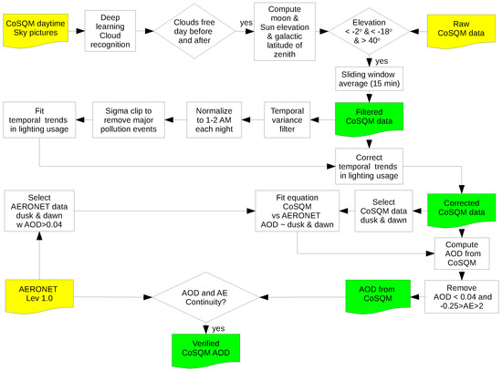
Figure 1.
General methodology used to derive the aerosol optical depth out of the CoSQM cloud-free, moon-free and Milky Way-free night sky brightness. Boxes in yellow are input data, whereas green boxes are data produced using the method. The upper-left box mentioning the CoSQM daytime Sky pictures specifies that no nighttime pictures are taken because of the lack of sensitivity in low light of the RPi camera sensor.
2.2. Instrumentation
2.2.1. The CoSQM System
As shown on Figure 2, the CoSQM is a portable device which aims to sample the multispectral properties of nocturnal artificial light scattered by the atmosphere. It was designed by Aube’s group to estimate the spectral properties of the ZNSB. The CoSQM has a cylindrical shape with a diameter of 11.5 cm, a length of 37 cm and a weight of 1.25 kg. It is composed of a filter wheel with five different spectral transmittances in the visible range (clear, red, blue, green and yellow; see Figure 3 for each band’s spectral response) that is standing on a step motor in front of a Unihedron Sky Quality Meter (SQM). The SQM is a sensor dedicated to the monitoring of the nocturnal sky’s brightness. It is panchromatic, with a spectral response encompassing the visible domain with some residual sensitivity in the near infrared (NIR) region [6]. The SQM sensitivity is close to zero at 1000 nm. The SQM sensitivity from 400 nm to 1000 nm is denoted by the black continuous line in Figure 3. In the CoSQM, we use the SQM model LE (SQM-LE), which includes its own Ethernet interface. We decided to use the SQM in order to be backward-compatible with the large amount of SQM data acquired worldwide to date and considering its high sensitivity and resolution of 0.01 magnitude per squared arc second (MPSAS). This unit is an inverted logarithmic scale that represents the brightness density (per solid angle). Magnitudes were initially developed to characterize the visibility of stars at night. The darker the sky, the higher the MPSAS. The CoSQM device comprises a Raspberry pi (RPi) open source Linux computer. The instrument can be operated remotely via the SSH protocol and the data may be accessed via an integrated web server. The data from all the instruments belonging to our CoSQM network are automatically downloaded every day and stored in a public server. In the second version of the CoSQM, the RPI is configured in such a way that the wired network interface is dedicated to the internet connection, whereas the WiFi interface allows access to the system and the data from any mobile device located near the CoSQM. In version 1, the WiFi interface was not used. Table 1 presents the main properties of the CoSQM v1 and CoSQM v2 devices.
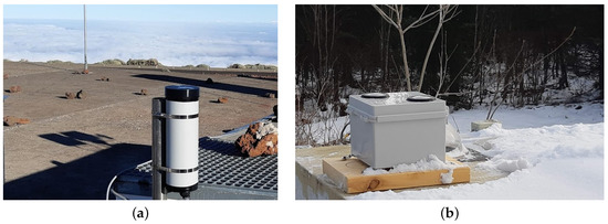
Figure 2.
The CoSQM device. (a) shows version 1 of the CoSQM. That specific unit is installed at AEMET Izaña observatory (Spain). (b) shows the second version of the CoSQM. This unit is installed at Saint-Camille (Canada).
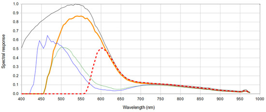
Figure 3.
Spectral responses of the CoSQM instrument installed at Santa Cruz de Tenerife. Shown are the relative spectral response of the 5 color filters installed in all the CoSQMs. The thin black line indicates the spectral response of the SQM-LE as measured in [6]. Other bands are consumer grade color filters in front of the SQM-LE. Colors are representative of the identification of the filters as per the manufacturer.

Table 1.
Feature comparison of CoSQM versions. The optional GPS sensor is identified with an asterisk.
The color detection capability is an important improvement over existing non-imaging detectors. This is particularly important in the context of the drastic change currently occurring in the color of light pollution, associated with the transition to light-emitting diode (LED) technology. The CoSQM’s developing philosophy is based on an open science model, in which all information is provided under an open licence. The methods, drawings, software and documentation can be accessed on the website of Pr. Aubé [7].
2.2.2. CoSQM Network
The CoSQM was designed to be used in a permanent installation mode in order to allow the implementation of a worldwide night sky color detection network. Nevertheless, it is possible to use the CoSQM as a moving device but in such a case a GPS need to be installed. Moreover, one should move slowly because the data acquisition is done every 2.5 min. Since its first release in 2018, 8 CoSQMs have been installed. These devices are located in a variety of sites, concentrated in Canada and Spain. Table 2 gives the list of instruments at the moment of writing and Figure 4 gives their mapped locations. We have indicated in bold the device used in the present paper. The Université de Sherbrooke site is noteworthy because there is also a star photometer installed nearby; therefore, we will eventually be able to compare our method with this measurement technique.
Table 2.
Instruments installed as part of the CoSQM network.

Figure 4.
Map of the CoSQM network. The station used for this study is highlighted in red.
2.2.3. AERONET Sun and Moon Photometers
The sun-sky-moon multi-band photometer CE318-T [8,9] is nowadays the only commercial instrument that is able to perform day and nighttime photometric measurements using the sun and the moon as a light source. The CE318-T is currently the reference instrument for AERONET, together with the old CE318-N standard version [10]. The new photometer version provides additional and enhanced operational functionalities compared with the standard CE318-N [1], mostly related to the improved tracking precision in terms of a new and more sensitive four-quadrant detector in the sensor head and a new control box which uses microstepping technology to improve the pointing resolution. Similarly to the CE318-N, the CE318-T version performs photometric measurements using nine interference filters, with nominal wavelengths centred at 1640 nm, 1020 nm, 937 nm, 870 nm, 675 nm, 500 nm, 440 nm, 380 nm and 340 nm. The CE318-T has an FWHM of 2 nm (ultraviolet, UV), 10 nm (visible, VIS) and 40 nm (near-infrared, NIR) (whereas the CoSQM has an FWHM of 50 nm for each band). Two photodiode detectors allow measurements in the ultraviolet, visible and near infrared spectral range (up to 1020 nm with a silicon detector) and in the near infrared and short-wave infrared range (at 1020 nm and 1640 nm with an InGaAs detector). Photometric measurements performed in the ultraviolet range are restricted to the daytime period, due to the low signal in the UV channels at night. The approximate field of view of the CE318-T is 1.29.
Once the feasibility of the Cimel CE318-T photometer to retrieve AOD at nighttime from lunar observations was assessed [8,9,11,12] a “provisional” lunar AOD product was released on the AERONET website. However, the AERONET team recognized the presence of anomalies in the data and they do not recommend its use for scientific publications [13]. This is why no presentation of the lunar product is provided in this work.
2.2.4. Meteorological State Agency of Spain (AEMET) Facilities
Three of the eight CoSQMs that form the network described in Table 2 were installed in AEMET facilities. This is the case for the stations at Santa Cruz de Tenerife (28.47N, 16.25W, 52 m a.s.l.), Izaña Observatory (28.31N, 16.50W, 2401 m a.s.l.) and Pico Teide (28.27N, 16.64W, 3552 m a.s.l.), located in Tenerife (Canary Islands, Spain), managed by the Izaña Atmospheric Research Centre (IARC) [14]. The subtropical location of this archipelago entails the existence of a strong temperature and moisture inversions in the lower troposphere [15], modulated by quasi-permanent subsidence conditions at this latitude as a result of the descending branch of the Hadley cell. As Carrillo et al. [15] found, one or two sharp temperature inversions or transition layers below the 700 hPa level can be found in the lower troposphere, limiting the humid and well-mixed marine boundary layer (MBL) to the dry and clean free troposphere (CFT) above. The top of the MBL, as an interface between these two very different air masses, is readily visible by the presence of quasi-permanent stratocumulus clouds frequent at this latitude, which have a critical role in preventing the arrival of anthropogenic and light pollution from lower altitudes. Another critical feature of Tenerife is its proximity to the African continent, entailing a strong influence of Saharan desert aerosols in the climatology of the three stations. The archipelago is located within the dust transport mainly during summer, as an elevated dust layer (the Saharan Air Layer or SAL) transported above the MBL at subtropical latitudes with a strong impact on the subtropical free troposphere over the North Atlantic [16,17,18]. Sporadic dust outbreaks can also affect the islands in winter, mostly restricted to lower levels, within the boundary layer [16,19]. These dust events are called “Calima”.
Santa Cruz de Tenerife Observatory is an urban station located within the MBL, close to the city harbor. As a consequence, the aerosol regime at this station is dominated by coarse mode sea-salt aerosols that are well mixed with fine-mode anthropogenic pollution, formed as a mixture of different anthropogenic sources [20,21,22]. Mineral dust particles also influence the aerosol climatology at the station, mainly from spring to autumn [21] but also in July–August [22]. As observed in Rodríguez et al. [23], the urban scale transport of air pollutants in this station is mainly driven by breeze circulation. Guirado-Fuentes [24] provides a complete aerosol characterization of this site. This author found that the AOD at 500 nm is typically lower than 0.15 and the Ångström exponent (AE) calculated using 440–870 nm spectral bands is lower than 0.5. These maritime clean conditions are observed over 60% of the year. An example of the steady conditions present at this site is shown on the Lidar product in Figure 5, which shows the normalized relative backscatter obtained from the MPLNET Lidar located at the same facility (https://mplnet.gsfc.nasa.gov/, accessed on 8 January 2021). The pictured conditions are representative of the typical conditions at the end of spring, one in a multitude of cases in which the proposed method is assumed to be valid since the AOD shows minimal variations throughout the night (0.05 maximum difference from the mean on 23 May to 24 May 2020, inclusively). Furthermore, the planetary boundary layer’s altitude is shown to be around 4 times compared to the aerosols altitude, which implies this location is a good candidate to evaluate the impact of higher aerosols on the determination of AOD from ground-based light sources.
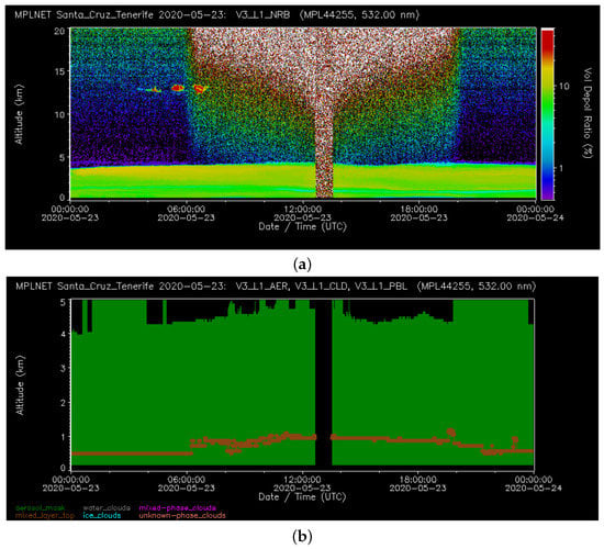
Figure 5.
Lidar volume depolarization ratio and aerosol inversion for 23 May 2020, in Santa Cruz de Tenerife, extracted from https://mplnet.gsfc.nasa.gov/, accessed on 8 January 2021. (a) shows a stable VDR signal throughout the time interval, notably at dusk and dawn and which represents the ideal conditions for the AERONET-CoSQM correlation based on steady temporal conditions. (b) shows the aerosol top layer height (green), as well as the planetary boundary layer (PBL) height (terracotta). The height of the aerosols above the PBL makes this period a good candidate to evaluate the method’s sensitivity to high-altitude atmospheric components. The CoSQM-measured AOD must depend upon the total atmospheric vertical layer to be compared to the AERONET sun photometer measurements.
Izaña and Teide Peak Observatories are two free troposphere stations, mainly characterized by clean background conditions, especially at nighttime, when the subsidence flow is reinforced. The predominant pristine conditions at the sites explain the historical importance of Izaña as a reference station for in situ and remote sensing atmospheric measurements, being designated by the WMO as a CIMO test bed for aerosols and water vapor remote-sensing instruments [25]. The two high-mountain stations can be sporadically affected by dust-loaded Saharan air masses mainly in summer, impacting the subtropical free troposphere [16,17,18]. As described in Guirado-Fuentes [24], researchers performed a detailed aerosol characterization at Izaña, finding that predominant clean background conditions are observed at the station (48% of the year with AOD at 500 nm below 0.05), whereas dust conditions can be associated with AOD at 500 nm higher than 0.10 and large particles with AE values lower than 0.60. These contrasting atmospheric conditions allow the methodology presented in this paper to be performed under a wide range of AOD values: from pristine to moderate dust loads.
2.3. Selecting the Most Relevant CoSQM Bands for Santa Cruz de Tenerife
In order to estimate the effect of the typical sky spectrum in combination with the filters’ spectral transmittance on the evaluation of the effective wavelength of the different CoSQM bands, we proceed to the modeling of the sky spectrum in Santa Cruz de Tenerife. We used the light inventory definition for Santa Cruz de Tenerife ([26]) with a neutral ground reflectance of 10% and the atmospheric content defined by the average AOD and AE (0.196 and 0.504, respectively) of the entire filtered dataset, as explained in the following subsection. This simulated sky spectrum is shown in Figure 6a. The minimal value of that spectrum represents the contribution of the natural star background. This spectrum has been adjusted using a city sky spectrum acquired in Huntington Beach (USA) and by scaling it to fit the differences between the sky brightness values given by the New World Atlas of Light Pollution [27] for the two sites. Then, to find the typical spectral signal detected by the CoSQM, we multiplied that spectrum with each band’s spectral transmittance from the CoSQM (3). The resulting effective spectral response is shown in Figure 6b. This result corresponds to a lamp’s inventory, which contains 90% high-pressure sodium (HPS), 5% metal halide (MH) and 5% LED 4000K. Figure 6c shows the effective spectral response for a city solely using LED lamps with a color temperature of 4000K. The effective wavelength of each CoSQM band is then estimated using a weighted mean of the product of the simulated sky spectrum with the band’s sensitivities. That process gave approximate values of red, green, blue, and yellow (RGBY) of 652 nm, 599 nm, 532 nm and 588 nm, respectively. Even if the spectrum of the sky changes slightly from one day to another, it will not significantly influence the calculated effective wavelength. According to our simulations, the effective wavelength cannot change by more than 10 nm under a change of lighting inventory. This is because city lighting relies only on a few different technologies (e.g., HPS, MH, LED). Therefore, these values were used as the CoSQM bands’ wavelengths in this particular case. It must be noted that this methodology must be redone for every site since the lamp inventory depends on the location.
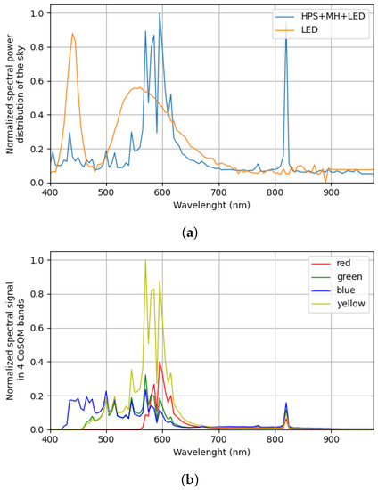

Figure 6.
Simulated spectra of the sky for a typical sky at Santa Cruz de Tenerife, and the respective spectral signal perceived by each CoSQM band. (a) shows in blue a simulated spectrum of the sky based on the lamp technologies in this location (HPS, MH and 4000K LEDs, [26]). A second sky spectrum is shown in orange, where all lighting devices are assumed to be 4000 K LEDs. The natural background is observed as the smallest sky brightness value in the graph, obtained with data from the World Atlas of Light Pollution to fit the measured natural sky brightness in Tenerife. (b) shows the effective spectral signal for each of the 4 color filters of the CoSQM, which takes into consideration the previous sky spectrum and the spectral response of each filter. The effective wavelengths are presented in the legend. (c) shows the effective spectral signal for the hypothetical case of the sole use of 4000K LED lighting on the basis of the LED sky spectrum of (a).
One can see in Figure 6b that the yellow band’s effective sensitivity is very wide, which renders it unusable for this work. In addition, the effective wavelength of the green and the yellow bands are very close to each other (599 nm vs. 588 nm); thus, no significant new information is obtained by using both, hence the discarded green band. The two bands having the most different effective wavelengths are the red and blue bands (652 nm and 532 nm), which motivated our choice to analyze only these bands for the determination of the AOD. Moreover, an analysis of the correlations between measured signals in all two-band combinations is shown in Figure 7. The plot clearly shows that the combinations showing the least correlations are the ones involving the red channel. Indeed, its effective signal is more restricted in the spectral domain (Figure 6b). Finally, only the blue channel was chosen as a second band because it represents the most different part of the whole spectrum and is sensible in higher wavelengths than the green and yellow channels.

Figure 7.
CoSQM band correlations. The correlation plots show that the best distinction is obtained with the red band. Considering that the most different band in terms of spectral sensitivity is the blue filter, only this one has been conserved for the rest of the work.
2.4. Filtering CoSQM and AERONET Data
To determine the AOD correlation, data points must be filtered for the presence of undesired sky brightness contributions so that the remaining variations are solely attributed to the AOD. In this work, data filtering was applied to the CoSQM instruments only, followed by the comparison with the CE318-T Level 1, respecting the same filtering. Moreover, the filtering time is reduced if one assumes that the CE381-T instruments are subject to the same sky conditions as the CoSQM, which is the case in this paper. The order in which the different filtering steps are presented is based on the order in which filters are applied in the calculations of the code and is optimized for computing time. Indeed, the cloud filtering sliding window is sensitive to consecutive values and must be performed within the first steps, before any other filtering is applied (or else filtering artefacts emerge).
2.4.1. Clouds
The presented method uses 3 different successive cloud filtering techniques, explained below:
- Machine learning cloud recognition: A multi-step algorithm has been written to determine the presence of clouds in rpi cam pictures taken at intervals of 15 min during daytime on each CoSQM. The combination of a residual network (ResNET) and a cyclic generative adversarial network (CycleGAN) generates a binary picture in which clouds are detected from the background. Simply put, RESNET+CycleGAN changes the whole original picture through a deep convoluted network to isolate the elements’ signatures (clouds, background) while finding the specific pixels where each signature is present. The combination returns a product that is tested with an adversarial network compared to 2 tagged sets of images (clouds/no clouds). The confirmation dataset is easily created with the rapid human visualization of a random subset of pictures, classified into 2 distinct groups. Following the training of the model, all pictures are transformed by the resulting function and a count of the cloud-contaminated pixels is made for each picture. Since a picture is taken every 15 min, these results provide information on cloud density over time. A threshold of cloud density per picture per day is then applied, which represents the criterion for the first cloud screening. If 90% of the data pixels are cloud-free both the day before and the day after a night of measurements, all data points for this night are conserved, or else removed. This percentage was determined based on a visual analysis of a 30% random subset of the entire Santa Cruz de Tenerife dataset containing 21,588 images, where the temporal variance described below was used to evaluate the presence of clouds for these nights. The results of the algorithm convergence after 30,000 epochs are presented in Figure 8, where the original pictures are first transformed to binary clouded/non-cloudedpixels and finally an attempt at cloud removal is undertaken with the same algorithm. This last step is not used in this project but was an interesting attempt at correcting pictures containing clouds. It also serves as a verification tool, since if the end picture appears to be cloud-free via a visual analysis, the cloud detection works. It must be noted that this corrected product has not been shown to be valid enough to be chosen as a filtering criterion in this work since the preliminary results were inconclusive. The accuracy of this method has been estimated at 85%, since the standard machine learning evaluation criteria of precision has not been applied to this specific algorithm. This value has been empirically determined by looking at 100 random results and qualifying each one on a scale of 1 (bad) to 5 (good). Further evaluation work on this approach shall show the best and worse conditions for applications.
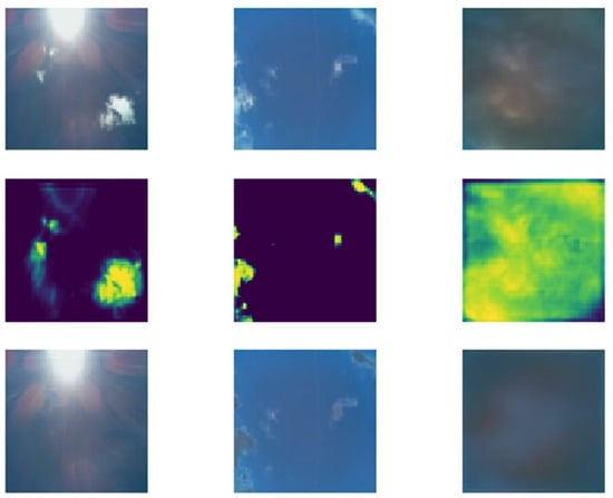 Figure 8. Machine learning algorithm cloud filtering: A combination of a ResNET and a CycleGAN allows the conversion of an RPi cam image (top) into a density map of the computed cloud presence (middle), which is used to transform the original image into a cloud-free version (bottom). Images are analyzed the day before and after a night of measurements, then the CoSQM data are filtered if more than 10% of the images contain clouds. Although not used in this project, the corrected product could help to obtain cloud-corrected ZNSB data with nighttime images, once improved and trained with a bigger dataset.
 - Temporal variance: A sliding window filter of empirically selected width is applied after the above filtering is completed. Care must be taken in this step to not be too aggressive on the filtering, or the short and intense events of particle loading will also be filtered, such as short Calima events. It must be noted that these filtering parameters strongly depend on the study location. This is discussed later and represents a challenge, considering the small number of data points after all filtering steps are applied, which, in this specific location, equates to a total of 2698 data points per band from a total pre-filtered 100,160 data points (2.7%). The selected width for Santa Cruz de Tenerife is a 12.5 min interval, representing 5 measurements for each color band. This value was chosen as it removed the remaining high variance/low MPSAS values, while leaving the known Calima events in the dataset, thus adding high AOD values to the correlation function. Since this filtering is applied individually to each night, the first and last measurements of a night are not modified by the nature of the sliding window. This effect was found to be negligible for the correlation results discussed below. A challenge imposed by the instrument is the fact that the 644 nm channel shows a variance twice as large as the other channels. As seen in Figure 9, CoSQM measurements higher than 19.95 MPSAS show a large variance, which does not pass the temporal variance filter. To fix this problem, the filter only treats the clear band measurements (no filter) which offers a higher signal-to-noise (SNR) ratio. The data points of the other color bands are then filtered for the same moments for which the clear channel is filtered. We have confirmed that this high variance in the 644 nm band is also observed for other color bands when they reach the same value close to 20 MPSAS. This seems to indicate that the sensors’ sensitivity exhibits low SNR for measurements higher than this value. Since the MPSAS scale is logarithmic, the higher the values the more the noise will be magnified. This is the intrinsic behavior of this scale.
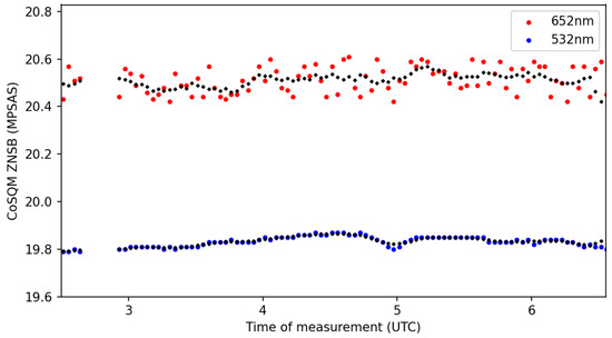 Figure 9. Different variance behaviors of the CoSQM filtered data after correcting for the lighting trends. The Figure shows the important differencse between high SNR values (blue band, 532 nm) and low SNR values (red band, 652 nm) for the night of 24 January 2020. Black symbols represent the data after applying a 15 min sliding average window over each associated color band.
 - Visual analysis: The data points filtered by the temporal variance filter can sometimes leave points that are most probably caused by a quasi-uniform cloud coverage of the entire CoSQM sensor (see Figure 8, right column, for an example). These points are in some cases indistinguishable from clear sky measurements; thus, a visual inspection of the sky pictures is needed. These points are first located in time in the entire dataset of CoSQM measurements and the specific images of the pi cam of the associated evening and the next day are visually examined and discarded if any of the two shows any definitive presence of clouds. A total of 13 nights of measurements were removed following this step, which represents 4% of the resulting nights contained in the dataset at this step.
As described above, cloud filtering steps are first run with very restrictive parameters to assure that the correlated points are as accurate as possible. From there, if the number of data points is not sufficient, the parameters are loosened to obtain more correlation values.
The filtering applied to the CoSQM also serves as the filtering criteria for the CE381-T data. Indeed, since the AOD measurements are taken during the day, the filtered dates for the CoSQM, primarily based on the presence of clouds, are also the same for the CE318-T. It must then be noted that the level 1 AERONET products are used for the CE318-T data, since the filtering has already been applied on the CoSQM (where level 1 means that no filtering has been applied). The use of level 1.5 or level 2 (increased filtering) would potentially remove high aerosol loading events, which are primordial to the correlation fit step of the method. The choice of using the level 1 products is valid based on the primary assumption of the project: AOD variations are slow in time and must be the same during dusk and dawn periods for the evaluation of continuity.
This filtering step left 42,050 of the 100,160 measurements (42%) of the entire CoSQM dataset in Santa Cruz de Tenerife, which indicates the important presence of clouds at this location and the emphasis on the cloud-screening techniques used in low-elevation sites. Measurements in this context mean a 5-value combination, one for each filter band (clear, red, green, blue, yellow).
The next generation of the instrument now incorporates a starlight camera, enabling the cloud detection algorithm to run during SQM measurements. This will allow a greater number of valid data points since the actual ML cloud screening process discards entire nights of measurements and not individual measurements.
2.4.2. Milky Way
Following previous filters, the next contribution to be addressed is the presence of the Milky Way in the instrument’s field of view. This step comes before the sun and moon filtering, since it removes more data points, thus reducing the computation time of the following steps. From an initial analysis of the data, the passage of the Milky Way in the field of view of the instrument can cause a ZNSB reduction of 0.7 MPSAS. By tracking the angle between zenith and the galactic plane (galactic latitude of zenith) using the Skyfield library and limiting its angle from the zenith at a threshold of 40 degrees, this filtering left 7460 of 100,160 measurements (7.4%) of the total data set in Santa Cruz. Considering the limited amount of data available to achieve the aimed goal, we decided to reduce this constraint to 30 degrees, leaving 9.5% of the initial data, an increase of 28% of the dataset size. The impact of this choice is calculated by taking the average of all the data that passed through every filtering step, resulting in a mean clear-band sky brightness difference of 0.08 MPSAS (7.6%) between the 40-degree case and the 30-degree case. The results were similar for the four color bands.
2.4.3. Moon
After the sun, the presence of the moon is the second most important light source to be assessed. Following the same process and using the same Python library, data points are removed if the moon’s elevation angle is higher than −2 degrees. This value has been determined via a visual inspection of several night measurement series for different moon illumination percentages throughout the period of study. This value is optimized to conserve the most data points while making the moon’s brightness contribution to ZNSB as small as possible, in this case in the order of 0.01 MPSAS. After this step of filtering, 5453 of 100,160 measurements (5.44%) were left of the entire dataset. This MPSAS value is less than the contribution of the Milky Way described in the previous subsection (0.08 MPSAS) and is explained by the fact that using a less restrictive value for the moon elevation did not increase the dataset size enough to justify the increased uncertainty caused by the moon’s contribution to ZNSB, as compared to the Milky Way.
2.4.4. Twilight
The scattering and refraction effects of the sun’s rays with the atmosphere near sunset and sunrise increase the sky brightness measured by the CoSQM. The filtering of this contribution is assessed by computing the sun’s elevation angle and removing all data points where this angle is higher than 18 degrees below the horizon. The Skyfield Python library was used to compute these angles [28]. This step of the filtering left 4987 of 100,160 measurements (5.0%). This small contribution to filtering is a consequence of the temporal variance filter that removes the rapidly changing ZNSB data points at sunset and sunrise. The initial evaluation indicates that this value can be extended up to −15 degrees for all sites located on Tenerife before an important sky brightness variation is measured. However, this higher angle only adds 2% of data points. It is not yet confirmed if other sites also show this behavior. Figure 1 specifies a sun angle filtering value of −18 degrees for generality purposes, since this is the most restrictive value in astronomy and is used in this work. Figure 10 shows the data reduction throughout the above defined filters. The initial measurements from the raw data were caused by instrument and/or network failures.
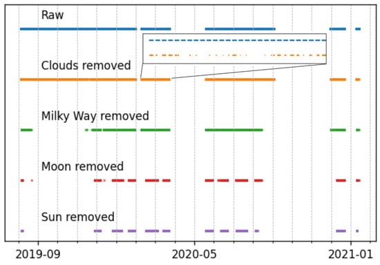
Figure 10.
Data reduction through cloud, Milky Way, moon and sun filtering. The raw data were successively filtered so the only important ZNSB contribution source left was light pollution emitted by artificial lighting. The size of the markers does not allow one to properly see the effect of the cloud-screening filtering but a zoom view is provided to outline the reduction following cloud removal.
2.4.5. Sliding Window Averaging per Color Band
As mentioned before, the SQM sensor experiences low SNR for high MPSAS measurements. To correct this situation, a second sliding window filter is applied on each band individually for all the datasets. The window duration of 15 min (7 measurements) proved to be optimal to reduce the variance while not averaging out the small-scale variations. As seen in Figure 9, the measurements above 19.95 MPSAS show a high variance compared to the lower values for this specific night. This value is not purely a consequence of the sensors’ sensitivity since the value at which the variance increases changes throughout the year. This could be explained by aerosol scattering during darker nights in the bands that exhibit the lowest signal (644 nm mostly). The Figure also shows that the filter adequately reduces the negative impact of the high variance in the 644 nm band.
2.4.6. Removal of Recurring Temporal Trends
Since the ZNSB depends greatly on light pollution sources close to the CoSQM site [29] and scattered light from light fixtures is the principal source of the signal, the temporal trends of lighting usage must be determined to correct for variations in sky brightness associated with human activity or light usage. This information can be extracted directly from the CoSQM filtered data (before the sliding window average step shown in Figure 1). To do so, CoSQM data are evaluated individually for ZNSB as a function of local time of night for each day of week, week and month of year and season. Variations between intervals are evaluated and the longest satisfying interval is chosen to simplify the relationship, while not overfitting the data. This is possible through the use of a low-order polynomial fit which is iteratively applied while excluding the data points that exceed one standard deviation from the resulting fit. This process ends when the final standard deviation converges to 0.1% of the previous obtained value, indicating that the removal of more data points is useless. In this way, we limit the fit sensibility to the random events that do not represent local lighting trends and are potentially caused by the presence of aerosols; thus, they should not have a major effect on the fit function. This iterative fit influences the ZNSB correlation points, which in turn influences the AOD from the ZNSB product. The iterative fit caused a mean variation of 6% on the final AOD values compared to a simple 3rd order fit of all data, where the majority of the modified values are related to ZNSB measurements taken before midnight (where the outliers of Figure 11 are mainly located). The impact of the iterative fit depends on the outlying points for a given dataset; it is then expected to vary at other locations. Finally, the nighttime-dependent contribution to ZNSB is removed from the filtered data. Following this evaluation, we compute a 3rd order correction per band, which is applied to the entire data set. The ZNSB is first averaged between 1:00 A.M. and 2:00 A.M. local time for each night. Each night is then normalized with this average and a 3rd-order function is fitted to the result. The fitted function is then subtracted from the ZNSB data as shown on Figure 12a for a specific night. For these specific datasets, the 1:00 A.M. to 2:00 A.M. time interval showed the least variations of ZNSB throughout the nights; therefore, it was chosen as the reference to normalize the ZNSB trends. This interval may vary between sites, but similar characteristics of lighting trends would probably be found in near cities, since lighting trends are correlated to population habits and customs and it is reasonable to assume that the darkest moment of the night happens in its middle. This interval is also the most likely to give accurate AOD values since it presents the least anthropogenic variations in ZNSB. The Figure also shows major differences in the fit parameters for the 644 nm channel compared to the others. This can be caused by a majority of street lighting technologies that present a lower color temperature such as high-pressure sodium and phosphor-converted amber LED bulbs (redder technologies). Compared to privately owned lighting, the public portion has a steadier contribution to sky glow since the street lights only turn on once per night. The increase in ZNSB around 4:00 A.M. can be explained by the private lighting habits of near sources such as bars, restaurants and other nightlife industries that typically close around that time in Tenerife. Finally, the lower end-of-night reduction in ZNSB for the 644 nm band seems to indicate an opposite relation compared to the results presented in [30], where cloudless nights’ ZNSB variations were observed to decrease more in the longer-wavelength bands than the smaller. The results of Kyba et al. [30] were obtained in Berlin, Germany.

Figure 11.
Night trends in lighting habits and their respective fit functions. Continuous lines indicate a 3rd order fit and dotted lines indicate an iterative weighted fit, which neglects values that show an offset higher than one sigma to the 3rd order fit, until the standard deviation of these values converges to 0.1%. (a) shows the correction of the normalized ZNSB for the 652 nm band filtered data. Density shows the number of points for each brightness value through the night and the fitted third-order night trend. The 3rd order fit was chosen since it adequately follows the lighting trends in urban locations. (b) shows similar results for the 532 nm band, although the effect of the correction is accentuated in this band.
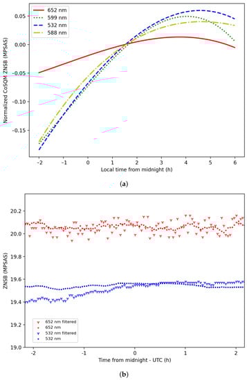
Figure 12.
Correction for the light usage trends. (a) shows a comparison of the correction functions for each CoSQM color filter band. (b) shows an example night of CoSQM ZNSB data for the night of 23 May 2020, for 2 cases: Filtered data (y symbols) for the presence of the sun, moon, Milky Way and clouds, as described in Section 2.4. Circles are filtered data, in which the high variance is removed with a sliding window, as described in Section 2.4.5 after applying the correction for light usage trends, as described in Section 2.4.6.
2.5. Fitting the AOD vs. Sky Brightness Relationships
Following the filtering steps, only a fraction of the data can be used to derive a relationship between AOD and ZNSB. Indeed, the AOD variation period required by the proposed technique must be greater than the interval between the last AERONET AOD measurement (typically 8:00 P.M.) and the first CoSQM measurements after filtering steps are applied (typically 10:00 PM). This implies that only a subset of the remaining data points are valid correlation candidates; in other words, successive nights and days are necessary to obtain reasonable results. The chosen method consists of the correlation of an average of AOD values around 5 h before dawn to an average of ZNSB values around 5 h after dawn (and inversely for dusk). Following the assumption that AOD variations happen on a bigger time scale than this 10 h interval limit, the ZNSB measured after dawn with the CoSQM should be correlated to the AOD measured before dawn with the CE318-T and inversely for dusk. This approach is intrinsically optimized for steady-state AOD conditions (i.e., where the AOD changes slowly). Dispersion of the points would be caused by rapid fluctuations of AOD happening close to dusk and dawn, which is not desirable. These points must be removed since there is no way to confirm that the correlation is in fact valid at these moments in time (AOD changes before the first ZNSB measurements are made, reducing the relation’s validity).
Since neither instrument has the same multispectral responses, the AE extracted from AERONET products is used to derive the AOD for each CoSQM nominal wavelength following Equation (1):
where is the AOD at the specific band’s CoSQM nominal wavelength, is the AOD at the specific band’s CE318-T central wavelength, is the specific band’s CoSQM nominal wavelength, is the specific band’s CE318-T wavelength and is the AE from the CE318-T for wavelengths in the 440–870 nm range. Since the AE also varies in time, the average of the values is also taken along with the CE318-T AOD measurements and this value is used in the above equation. The following equation was chosen to fit the AERONET AOD to the CoSQM ZNSB:
where a and b are parameters determined for each site. The choice of the function is based on the fact that the magnitude scale is a function of the logarithm of the radiance of the sky, which should be reflected through the AOD dependence. Although AOD would be expected to be linearly dependent on ZNSB, such a fit function did not give good results for small AOD values and the deviation from these low values was 5 times higher than for AOD values close to 1. Furthermore, falls to 0 at a finite brightness, which is assumed to be the ZNSB of the natural sky radiance plus the minimal sky radiance produced by molecules without any aerosols for a given site. Hence, this 0 point will vary between sites that exhibit different lighting conditions. Molecules can also scatter light without the presence of aerosols, which may vary according to the sources of artificial light around the site. It is important to note that the fit function is only valid for a specific interval of ZNSB, which depends on the site for which the fit was obtained. Indeed, the chosen function rapidly decreases towards small AOD values in the range of 0.01 for small ZNSB variations in the range of 0.1 MPSAS, often allowed by the low SNR, high ZNSB measurements in the 644 nm band. However, the range of sky brightness considered in this approach does not allow such low values to be reached (SB is always higher than 17 MPSAS for Santa Cruz de Tenerife in the selected dataset). This then implies that the magnitude scale for each site is bounded in respect to the local light pollution.
3. Results
3.1. AOD–ZNSB Correlations
The correlation results obtained through the above filtering steps are presented in Figure 13a for Santa Cruz de Tenerife. Rational functions are fitted to the data using a non-linear least squares method. This choice of function was made based on the possibility of a non-negative AOD value, as well as a decreasing AOD value as a function of sky magnitude. As seen in this figure, a distinction exists between the dusk and dawn correlation points, which could be explained by the relative humidity variations throughout the night. It is expected that water-soluble or hydrophilic aerosols, especially marine ones, change their size by absorbing water. This change in size impacts the AOD [31]. This phenomenon is coherent with the relative humidity (RH) statistics for dusk and dawn at Santa Cruz de Tenerife. As shown in Figure 13b, RH is generally higher at sunrise, which implies a larger particle size. This may be linked with increased AOD without a change in particle number density. Separate correlation functions have been evaluated but did not result in better AOD-ZNSB and AE continuity, so were ignored in this initial analysis. Furthermore, RH must not be the only parameter that creates a distinction between dusk and dawn correlation points. Without further analysis of this behavior, we decided to fit a single function per band for the entire dataset. Each band used 51 data points to determine the correlation. For a preliminary evaluation of the interaction of atmospheric particles (aerosols and molecules) and the ground-located sources at the location of Santa Cruz de Tenerife, a simulation of the Illumina model was made with exponential decreasing aerosol layers of height parameters H = 2 km and H = 10 km. The results shown in Figure 14 demonstrate that the contributions to the sky radiance from aerosols above 2 km are respectively 2.04% and 6.53% of the total aerosol sky radiance. The contributions to the sky radiance from aerosols above 5 km are respectively 0.69% and 2.63% of the total aerosol sky radiance. Although small, these results confirm that ZNSB is influenced by high-altitude aerosols and the proposed method could be valid for different atmospheric aerosol profiles and not strictly restrained to the interactions in the planetary boundary layer (PBL). As described in [5], the relationship between ZNSB and aerosols and especially their attenuation as a function of the distance to light sources does not follow a simple law (the exponent of the function varies with distance). Indeed, the Illumina model has shown that in some situations, the 2nd order scatterings represent only a 7% contribution to sky brightness. This contribution decreases when the observer is closer to light sources. Furthermore, this contribution can reach up to 60% when farther from sources. Futhermore, correlation data points were obtained at different moments of the year, for which Santa Cruz de Tenerife exhibits various atmospheric conditions. The Lidar normalized relative backscatter (NRB) graphs represent the raw signal, which is then converted into different products, such as the volume depolarization ratio (VDR) and layer heights: aerosols (AER), clouds (CLD) [32] and PBL. As seen in Figure 15, winter brings clean maritime conditions, usually cloudy and with a PBL height around 1 km, respectively, represented by red zones on the VDR plot (middle rows) and by terracotta-colored points in the layer plot (lower rows). As seen in Figure 16, winter time can also bring dust at lower levels, typically below 2 km, represented by turquoise zones in the VDR plot. These conditions usually imply an aerosol-free troposphere, as seen in the AER layer product. In summer, mainly July and August, dust events can reach up to 6 km and these conditions are referred to as the Saharan Air Layer (SAL), as pictured in the VDR plot in Figure 17. The free troposphere, referred to as the clean layer, appears above this altitude. Although the Lidar data precisely matching the dates of the ZNSB measurements was only available for the week of 7 June 2020, in SAL conditions, the conditions at Santa Cruz de Tenerife exhibit seasonal cycles and it is highly probable that the correlation points are representative of a multitude of typical atmospheric conditions. These SAL conditions also help to conclude that the proposed method is valid for high aerosol loading at high altitudes.
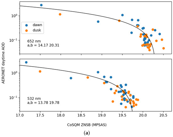

Figure 13.
Relationship between ZNSB and the daytime AOD. (a) shows the correlation plot between AOD from the CIMEL CE318-T sun photometer and ZNSB from the CoSQM multispectral sensor for the Santa Cruz de Tenerife location. The filtered and averaged data are fitted using Equation (2). Parameters a and b correspond to the fitted parameters in this equation. The dusk and dawn legend specifies the period represented by each value. (b) shows the relative humidity histogram at sunset and sunrise for the year 2020 in Santa Cruz de Tenerife. The higher values associated with sunrise (dawn) explain the difference in the plotted points shown in (a) since higher relative humidity may be associated with higher AOD values.
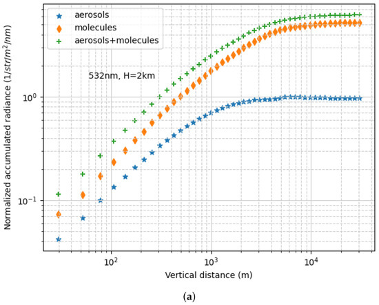
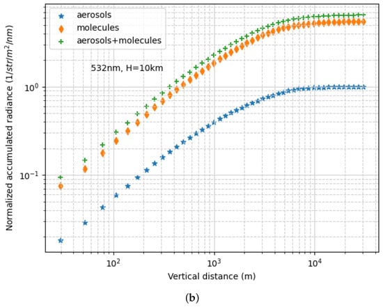
Figure 14.
Accumulated radiance as a function of elevation, normalized to the aerosol total contribution. These contributions are respectively for H = 2 km and H = 10 km and W/str/m2/nm. The values were obtained with the radiative transfer model ILLUMINA v2 for Santa Cruz de Tenerife in the case of (a) aerosol layer with vertical scale height of 2 km and (b) an aerosol layer with vertical scale height of 10 km. The aerosol contribution was obtained by subtracting the simulation with an AOD value of 0.13 to the simulation with an AOD value of 0, with a constant RH value of 70%. The graphs show a non-zero contribution of high altitude aerosols (>5 km) to the total radiance and consequently to the total ZNSB. These results indicate the method of AOD retrieval from ZNSB should be sensitive to the quasi-total aerosol layers.
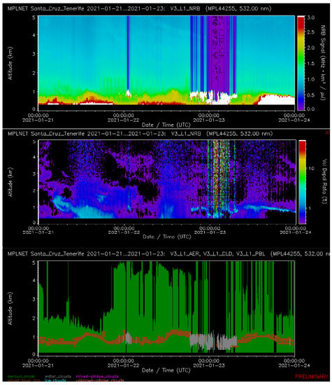
Figure 15.
Clean winter conditions with low aerosol loading around 22 January 2021.
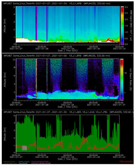
Figure 16.
Lidar products from AERONET showing the NRB above and the particulate discrimination vertical profiles as a function of time. Noisy vertical lines are the consequence of the closing dome to mitigate direct sunlight to the sensor. The Figure shows dust-dominant winter conditions around 29 January 2021.
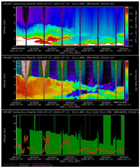
Figure 17.
Lidar products from MPLNET for summer conditions. The Figure shows dust-dominant summer conditions around 10 July 2020.
3.2. Daytime vs. Nighttime Continuity
The time continuity of AOD can be evaluated for the heavily light-polluted case of Santa Cruz de Tenerife with the obtained correlation functions. The AOD is computed from the ZNSB measurements following the results of Figure 13a and Equation (2) for each band. The AE is computed following Equation (3). This approach is the same as the AERONET AE product (440 nm and 667 nm bands), although with different bands (532 nm and 652 nm).
where is the Angstrom exponent, is the AOD in the blue band, is the AOD in the red band and , are the blue and red bands’ nominal wavelengths. From these products, the AE is filtered following two quality-control criteria: (a) negative values smaller than −0.25 are rejected and (b) values higher than two are rejected based on the common high values observed at this location in the AERONET products throughout the data set period. This serves as a reference basis to determine which AE values are acceptable from the proposed method. The first threshold applied to AOD values is based on the precision of the sensor. As stated, the uncertainty of 0.01 mpsas of ZNSB is mapped to an AOD uncertainty of 0.04. Any smaller AOD value would potentially be caused by a ZNSB that, considering the uncertainty, could give a negative AOD. Of course, this is not physical. In this way, this threshold is not arbitrary and will not be identical for each site and moment where this method is used. The second threshold is based on the quality of the results obtained for the AE. This threshold is mainly explained by the presence of outliers and one can say it has a less solid basis. Based on the results shown below, the AE product validity from this method must be questioned. The filtered AE values are finally linked to the measurement dates, themselves used to filter the AOD computed values since non-valid AE values would indicate non-valid AOD values. The results are presented in Figure 18a, Figure 19a and Figure 20b. Considering the uncertain validity of the moon photometer-derived AOD nighttime values from AERONET at the time of writing, these products are not presented. Figure 18 shows the results of the continuity for both AOD and AE for the four color bands of the CoSQM with the equivalent AERONET sun photometer AOD in the week of 20 February 2020, during a Calima event. Figure 19 shows similar results for the week of 21 May 2020 for a calmer aerosol loading event. The associated AOD derived from the CoSQM data is in accordance with the daytime AERONET AOD, even in the case of a high uniform vertical distribution of aerosols. Good continuity results were also observed for SAL conditions, as shown in Figure 20, which confirms that the method is representative of higher-altitude particles (higher than the dense PBL). Although real, negative AE values are not common and they are usually retrieved in the limit of 4 (Rayleigh scattering) to 0 (large aerosols). The occasional occurrence of negative values can be associated with instrumental errors (low SNR situations). In fact, following Wagner and Silva [33], the uncertainty associated with AE values retrieved from sun photometers (with an expected AOD uncertainty between 0.01 and 0.02, as the case of the Cimel) is 1.17 for clean conditions and 0.17 for hazy conditions. There are other additional effects, such as the impact of forward scattering due to mineral dust measured by a finite field-of-view (FOV) photometer in certain conditions with coarse mode dominance (see [18] for further details). In this case, due to the FOV effect, the AOD measured is lower with particle size and wavelength. As a consequence, under these circumstances (FOV and coarse mineral dust), lower-than-expected AOD values are measured at shorter wavelengths, causing the AE values to be lower than real values. This was the case for a severe dust outbreak which took place in the Canary Islands in February 2020. This extreme event was the object of a publication [34], defined as an intense dust episode from the desert areas of the western Sahara towards the Canary Islands, with an important contribution of particulate matter higher than 6 m and a negligible fine mode. This is a consequence of the proximity of the dust emission source and the high wind speed in this particular dust episode. The AERONET control algorithms often incorrectly eliminate AOD events due to the intensity and speed of the dust intrusion affecting the observatory, incorrectly attributing them to the presence of clouds.
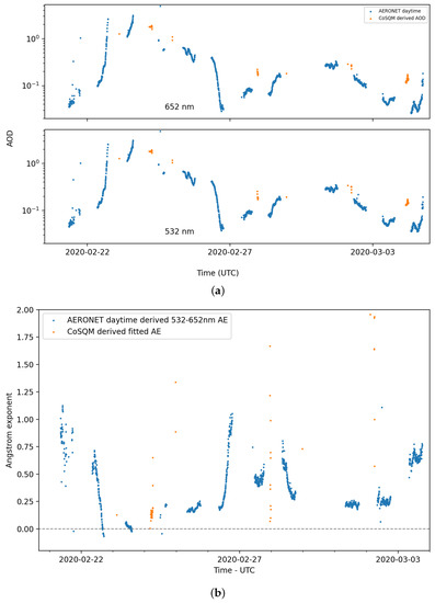
Figure 18.
Continuity of ZNSB-derived AOD and AE values compared to AERONET daytime sun photometer measurements during and after a Calima event. (a) shows the AOD for the 4 CoSQM bands and (b) shows the AE derived from a fit of Equation (3) on CoSQM AOD values compared to AERONET 440–675 nm daytime sun photometer measurements.
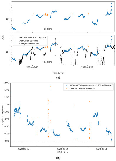
Figure 19.
As in the above Figure 18, continuity of ZNSB-derived AOD and AE values compared to AERONET daytime sun photometer measurements during typical conditions.
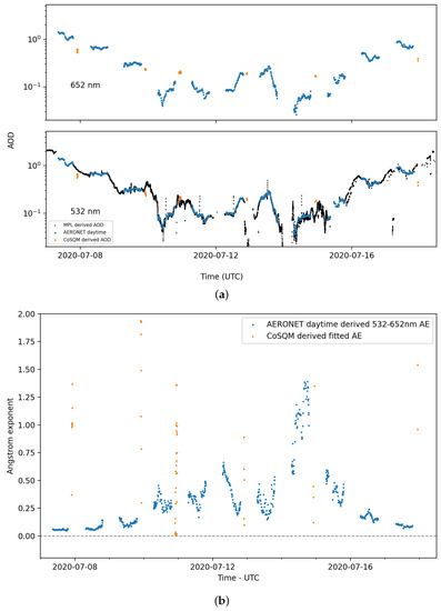
Figure 20.
Continuity of ZNSB-derived AOD and AE values compared to AERONET daytime sun photometer measurements during typical conditions. (a) shows the AOD for the 4 CoSQM bands and (b) shows the AE derived from a fit of Equation (3) on CoSQM AOD values compared to AERONET 440–675 nm daytime sun photometer measurements.
Variance throughout the typical night of 23 May 2020, is shown in Figure 21, where the method of the extremes is applied to evaluate the uncertainty of AOD, here 0.02. The selected night is representative of what is defined as stable-state conditions in the context of this work, which seems to indicate that this night is a good candidate to evaluate the AOD uncertainty. Finally, the theoretical dependency of ZNSB as a function of distance for multiple AOD values is shown in Figure 22a, as described in Simoneau et al. [5]. It can be seen that in cases where contributing light sources are located either near the observer (<2 km) or far from it (>20 km), a good determination of AOD is possible given the high dynamic range of values. Figure 22b then shows the radially integrated contribution maps for the AEMET research center of Santa Cruz de Tenerife. This plot was generated with the Illumina v2 [26,35] model using the light inventory developed by Aubé et al. [26]. As can be seen, 90% of the light source’s contribution is located in a mean radius of ≈2.5 km and 99% under ≈8 km. This indicates that this site is a good candidate for the proposed method because most of the contributing lighting devices are located in the low interval that presents a good discrimination of AOD, as determined based on Figure 22a.
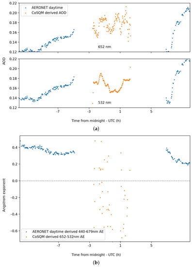
Figure 21.
Variance of AOD and AE for the steady-state night of 23 May 2020. In (a) an AOD uncertainty of 0.02 can be evaluated if the variations are not considered to be of physical origin. (b) shows the AE for the same night. The negative values can be caused by the high variance in ZNSB values for very dark sky conditions (higher than 19.95 MPSAS) or in the presence of high/low AOD values (1 or 0.05) caused by Rayleigh scattering or large aerosols.
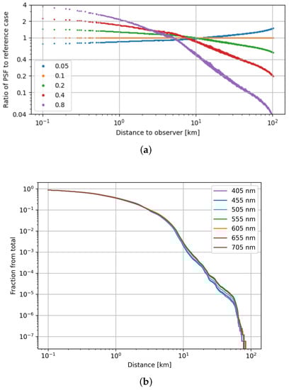
Figure 22.
Most important sources in relation to the ZNSB–AOD relationship. (a) shows the dependence of relative sky brightness with the distance from sources to an observer looking at the zenith for different AOD values. The modeled case is for lamps having a 5% upward light output ratio, a wavelength of 550 nm, an AOD of 0.1 and an Ångström exponent of 1.3. These figures come from [5]. The Figure indicates that the correlation function should better discriminate between various AOD values for sites having most of their light sources either near the CoSQM (<2 km) or far (>20 km) from it. (b) shows the fraction of the ZNSB coming from within a given radius. The plot is for the AEMET location of Santa Cruz de Tenerife, with an AOD value of 0.13 and an AE of 0.6 (representative of the average value for this site in 2020). Calculations were made with Illumina v2 model [26]. Contributions are shown for each simulated wavelength. Furthermore, 90% of the ZNSB is coming from inside a radius of ≈2.5 km and 99% from inside a radius of ≈8 km.
4. Discussion and Conclusions
In this paper we have presented an innovative method to determine the AOD at night by observing the light pollution scattered by the atmosphere. This new method appears to be promising, especially for heavily light-polluted sites with many nearby light pollution sources located within a few kilometres. This method adds new information on the optical properties of aerosols, and therefore it may have a significant impact in improving future global climate model predictions. The results show that the determination of AOD is possible for the specific site of Santa Cruz de Tenerife since it is a highly light-polluted site and the majority of the contribution of ZNSB from light sources is located within less than approximately 2.5 km, where the AOD dynamic range is high (see Figure 22a). This was also made possible since enough data points remained after the numerous ZNSB filtering steps, and an apparently realistic correction of the nocturnal lighting trends was obtained. The latter is of the upmost importance since it has a direct influence on the AOD values computed with the method. Indeed, if an ivalid correction is applied, the resulting AOD will not correlate with the AERONET product and will give high variance fit values, which have been shown to cause multiple problems (see the AE results in Figure 21b). The computed fit functions show high dispersion around small AOD values around 0.1. This is caused by the filtering parameters, which are set to obtain as much valid data points as possible for the correlation and to avoid a filtering bias (for example, keeping only summertime data points). A higher number of measurements would allow us to possibly reduce this dispersion, since filtering would be increased and confirm the above assertion. Furthermore, the upcoming version of the instrument, which has a more sensitive camera, will allow the short-time detection of the presence of clouds. The presence of clouds is thought to be the most influential factor in regard to the dispersion of the correlation function. Variations of the order of 100% exist between the dusk of a date and the dawn of the next morning. However, the correlation is limited to a time interval of 8–10 h (dusk to dawn) and high discrepancies would be observed in the correlation points if such changes were present, which are not observed. It must be noted that this time interval is the maximum limit, which is not often reached in the dataset. Furthermore, since no nighttime measurement exists for the nighttime AOD CoSQM retrievals shown (which was the main motivation of this work), it is impossible to evaluate if the AOD variations are not steady between AERONET and CoSQM measurements. Furthermore, one cannot even assume that successive days that show near 0% AOD variations are better candidates for correlation points since the AOD may change during the night and return to its earlier value before dawn. Based on this, we chose not to filter out any data points that remained after filtering and threshold steps. Since our method only works in the absence of the moon (lunar model correction will be evaluated in future work), any simultaneous comparison with this product is impossible. Indeed, only star photometer measurements can provide confirmation of the AOD derived from the method explained in this paper. These results will be part of future works. Nevertheless, we evaluated the method’s validity by comparing the AOD product obtained from ZNSB to the Lidar inversion product of the MPLNET. They showed good agreement, as shown in Figure 20a. In the case of the aerosol loading event presented in Figure 19a, the ZNSB product seems to overestimate the AOD, whereas the Lidar product seems to underestimate the AOD compared to the daytime sun photometer AERONET product. The variability of the measurements for a given night shown in this figure is higher for the Lidar product (which also contains more data points), which does not follow the daytime AOD evolution as coherently. Once more, no discrimination can be carried out without simultaneous comparison with the star photometer product. The uncertainty of the method for Santa Cruz de Tenerife can be evaluated based on Figure 21, in which the maximum variations are 0.02 for AOD and 0.75 for AE (although more analysis on the latter is needed to draw conclusions as to this value). This high value for the AE is thought to be caused by the low SNR measurements, primarily in the red band. Another factor is that the CoSQM color bands overlap each other, as seen in Figure 6b. This implies that the measurements are not independent from each other compared to the AERONET AE product (318-T narrow bands). However, Figure 6a shows that the effective spectral sensitivities are much more independent, at the cost of signal intensity. Considering the major conversions of light sources to LED technology around the world, the proposed method would have greater potential in these converted locations. The high variance in AE helps to distinguish the most valid computed CoSQM AOD values. As of now, our results seem to show considerable variations compared to AERONET but there is no way to conclude that they are erroneous without the use of nighttime AOD products from another instrument. The AOD uncertainty is based on the worst-case scenario since we believe nocturnal variations to be caused by physical phenomena, such as rises in relative humidity levels, as well as decreases in human activity throughout the night. The resolution of the SQM sensor is 0.01 MPSAS, which, according the correlation function, equates to an AOD of 0.05. This shows that the selected SQM sensor is adequate for the proposed method. Also, some nights show small AOD temporal variations of the order of 0.1 and a steady transition from one day to the other, which seems to indicate that the variations observed are not purely random and that the uncertainty would be lower than previously estimated for nights with low ZNSB (high SNR) values. The evaluation of the method in the three other locations on Tenerife Island (see Table 2) will be presented in a future work. It is not trivial if the method will work well for these sites because an important part of the light for at least Izana and Observatorio del Teide seems to come from sources concentrated around a distance of 10 km, which is the critical zone with almost no possibility of discriminating AODs, as shown in Figure 22a. In fact, these sites do not have significant sources of light pollution inside a radius of a few kilometers. Such situation may mitigate the possibility of distinguishing different AOD values. The case of Pico Teide may be different because in that case many contributing sources must be farther than ≈13 km, where the dynamic range for discriminating AOD values is high (see Figure 22a). On the other hand, the signal-to-noise ratio is expected to be lower given that the site is distant from sources, and therefore it is weakly light polluted. Future work will also aim to compare AOD results obtained from star photometry to the technique described in this paper. The advantages of this approach are the low uncertainty of the star photometer measurements (0.01 AOD with the two-star method [3]) and the same clear sky conditions for simultaneous data point comparisons. This would allow an absolute calibration and the uncertainty of the exposed method could be better determined. At the time of writing, a remote-controlled star photometer and a mini-MPL Lidar, part of the MPLNET Network, are being installed at the Sherbrooke site, listed on Table 2, for the above evaluation purpose. In combination with the CIMEL318-T also installed in Sherbrooke, the evaluation of the method in this location looks promising. Furthermore, the results a new product from AERONET based on the RIMO (ROLO Implementation for Moon Observation) correction factor (RCF) [36] method, giving precise AOD values from moon photometry, will be compared to our results. This addition to the continuity evaluation of AOD across years and sites would represent a better basis for correlation since the time interval between an RCF measurement and a CoSQM measurement would be greatly reduced. Finally, the replacement of the actual units with CoSQM V2 units will allow nighttime sky pictures to be taken for each measurement sequence (ultimately at an interval of 2.5 min), which will greatly increase the total number of data points after cloud filtering (compared to a cloud-free filtering frequency of about 36 h, or two consecutive days, applied with the CosQM v1 used in this study), increasing the accuracy of the method.
Author Contributions
We applied the sequence-determines-credit approach [37] for the sequence of authors, which is in order of decreasing contributions. Conceptualization, M.A.; methodology, C.M. and M.A.; software, M.A., C.M. and A.S.; validation, M.A. and C.M.; formal analysis, M.A. and C.M.; investigation, M.A., C.M. and A.B.; resources, M.A. and A.B.; data curation, C.M., M.A. and A.S.; writing—original draft preparation, M.A., A.B. and C.M.; writing–review and editing, M.A., C.M., A.B. and A.S.; visualization, C.M., M.A. and A.S.; supervision, M.A.; project administration, M.A.; funding acquisition, M.A. All authors have read and agreed to the published version of the manuscript.
Funding
M.A., C.M. and A.S. thank the Fonds de recherche du Québec—Nature et technologies (FRQNT) for financial support through the Research program for college researchers.
Acknowledgments
We want to thank Ramon Ramos and Antonio Cruz Martin from the AEMET office and Miquel Serra Ricart from the Instituto de Astrofisica de Canarias who helped with the installation of the CoSQM units on Tenerife Island. We also thank Normand T. O’Neill for his educated advice concerning this work, Marc-Antoine Genest for his help on the deep learning algorithm testing and Élysé Lapalme for his help on the cloud screening evaluation. This work was developed within the framework of the activities of the World Meteorological Organization (WMO) Commission for Instruments and Methods of Observations (CIMO) Izaña Testbed for Aerosols and Water Vapor Remote Sensing Instruments. The authors thank the MPL Network (MPLNET) for the Lidar aerosol profiles and the Aerosol Robotic Network (AERONET) for the aerosol optical data. The AERONET sun photometer at Santa Cruz has been calibrated within the AERONET Europe TNA, supported by the European Community Research Infrastructure Action under the FP7 ACTRIS grant, agreement No. 262254.
Conflicts of Interest
The authors declare no conflict of interest.
Abbreviations
The following abbreviations are used in this manuscript:
| AEMET | Agencia Estatal de Meteorología |
| AERONET | AErosol Robotic NETwork |
| AOD | Aerosol optical depth |
| CoSQM | Color Sky Quality Meter |
| FRQNT | Fonds de recherche du Québec—Nature et technologies |
| GPS | Global Positioning System |
| LED | Light Emitting Diode |
| MPSAS | Magnitude Per Square Arc Second |
| NIR | Near-infrared |
| nm | nanometer |
| RGBY | Red, green, blue, yellow CoSQM filter colors |
| RIMO | ROLO Implementation for Moon’s Observation |
| SNR | Signal-to-Noise |
| SQM | Sky Quality Meter |
| UPS | Uninterruptible Power Supply |
| UV | Ultraviolet |
| VIS | Visible |
| ZNSB | Zenithal night sky brightness |
References
- Holben, B.N.; Eck, T.; Slutsker, I.; Tanre, D.; Buis, J.; Setzer, A.; Vermote, E.; Reagan, J.; Kaufman, Y.; Nakajima, T.; et al. AERONET—A federated instrument network and data archive for aerosol characterization. Remote Sens. Environ. 1998, 66, 1–16. [Google Scholar] [CrossRef]
- Levy, R.C.; Mattoo, S.; Munchak, L.A.; Remer, L.A.; Sayer, A.M.; Patadia, F.; Hsu, N.C. The Collection 6 MODIS aerosol products over land and ocean. Atmos. Meas. Tech. 2013, 6, 2989–3034. [Google Scholar] [CrossRef] [Green Version]
- Ivănescu, L.; Baibakov, K.; O’Neill, N.T.; Blanchet, J.P.; Schulz, K.H. Accuracy in starphotometry. Atmos. Meas. Tech. Discuss. 2021, 2021, 1–58. [Google Scholar] [CrossRef]
- Aubé, M.; Franchomme-Fossé, L.; Robert-Staehler, P.; Houle, V. Light pollution modelling and detection in a heterogeneous environment: Toward a night-time aerosol optical depth retreival method. In Atmospheric and Environmental Remote Sensing Data Processing and Utilization: Numerical Atmospheric Prediction and Environmental Monitoring; International Society for Optics and Photonics: Bellingham, WA, USA, 2005; Volume 5890, p. 589012. [Google Scholar]
- Simoneau, A.; Aubé, M.; Leblanc, J.; Boucher, R.; Roby, J.; Lacharité, F. Point spread functions for mapping artificial night sky luminance over large territories. Mon. Not. R. Astron. Soc. 2021, 504, 951–963. [Google Scholar] [CrossRef]
- Sánchez de Miguel, A.; Aubé, M.; Zamorano, J.; Kocifaj, M.; Roby, J.; Tapia, C. Sky Quality Meter measurements in a colour-changing world. Mon. Not. R. Astron. Soc. 2017, 467, 2966–2979. [Google Scholar] [CrossRef]
- Aubé, Martin. CoSQM Webpage. 2021. Available online: https://lx02.cegepsherbrooke.qc.ca/~aubema/index.php/Prof/CoSQMEn (accessed on 8 January 2021).
- Barreto, A.; Cuevas, E.; Damiri, B.; Guirado, C.; Berkoff, T.; Berjón, A.J.; Hernández, Y.; Almansa, F.; Gil, M. A new method for nocturnal aerosol measurements with a lunar photometer prototype. Atmos. Meas. Tech. 2013, 6, 585–598. [Google Scholar] [CrossRef] [Green Version]
- Barreto, A.; Cuevas, E.; Granados-Muñoz, M.J.; Alados-Arboledas, L.; Romero, P.M.; Gröbner, J.; Kouremeti, N.; Almansa, A.F.; Stone, T.; Toledano, C.; et al. The new sun-sky-lunar Cimel CE318-T multiband photometer—A comprehensive performance evaluation. Atmos. Meas. Tech. 2016, 9, 631–654. [Google Scholar] [CrossRef] [Green Version]
- Giles, D.M.; Sinyuk, A.; Sorokin, M.G.; Schafer, J.S.; Smirnov, A.; Slutsker, I.; Eck, T.F.; Holben, B.N.; Lewis, J.R.; Campbell, J.R.; et al. Advancements in the Aerosol Robotic Network (AERONET) Version 3 database—Automated near-real-time quality control algorithm with improved cloud screening for Sun photometer aerosol optical depth (AOD) measurements. Atmos. Meas. Tech. 2019, 12, 169–209. [Google Scholar] [CrossRef] [Green Version]
- Berkoff, T.A.; Sorokin, M.; Stone, T.; Eck, T.F.; Hoff, R.; Welton, E.; Holben, B. Nocturnal aerosol optical depth measurements with a small-aperture automated photometer using the moon as a light source. J. Atmos. Ocean. Technol. 2011, 28, 1297–1306. [Google Scholar] [CrossRef]
- Li, Z.; Li, K.; Li, D.; Yang, J.; Xu, H.; Goloub, P.; Victori, S. Simple transfer calibration method for a Cimel Sun–MOON photometer: Calculating lunar calibration coefficients from Sun calibration constants. Appl. Opt. 2016, 55, 7624–7630. [Google Scholar] [CrossRef]
- Aeronet Technical Document. Lunar Aerosol Optical Depth Computation. 2019. Available online: https://aeronet.gsfc.nasa.gov/new_web/Documents/Lunar_Algorithm_Draft_2019.pdf (accessed on 8 January 2021).
- IARC. IARC Webpage. 2021. Available online: http://izana.aemet.es (accessed on 8 January 2021).
- Carrillo, J.; Guerra, J.C.; Cuevas, E.; Barrancos, J. Characterization of the Marine Boundary Layer and the Trade-Wind Inversion over the Sub-tropical North Atlantic. Bound.-Layer Meteorol. 2016, 158, 311–330. [Google Scholar] [CrossRef]
- Rodríguez, S.; Alastuey, A.; Alonso-Pérez, S.; Querol, X.; Cuevas, E.; Abreu-Afonso, J.; Viana, M.; Pérez, N.; Pandolfi, M.; de la Rosa, J. Transport of desert dust mixed with North African industrial pollutants in the subtropical Saharan Air Layer. Atmos. Chem. Phys. 2011, 11, 6663–6685. [Google Scholar] [CrossRef] [Green Version]
- Rodríguez, S.; Cuevas, E.; Prospero, J.M.; Alastuey, A.; Querol, X.; López-Solano, J.; García, M.I.; Alonso-Pérez, S. Modulation of Saharan dust export by the North African dipole. Atmos. Chem. Phys. 2015, 15, 7471–7486. [Google Scholar] [CrossRef] [Green Version]
- Cuevas, E.; Romero-Campos, P.M.; Kouremeti, N.; Kazadzis, S.; Räisänen, P.; García, R.D.; Barreto, A.; Guirado-Fuentes, C.; Ramos, R.; Toledano, C.; et al. Aerosol optical depth comparison between GAW-PFR and AERONET-Cimel radiometers from long-term (2005–2015) 1 min synchronous measurements. Atmos. Meas. Tech. 2019, 12, 4309–4337. [Google Scholar] [CrossRef]
- Cuevas, E.; Camino, C.; Benedetti, A.; Basart, S.; Terradellas, E.; Baldasano, J.M.; Morcrette, J.J.; Marticorena, B.; Goloub, P.; Mortier, A.; et al. The MACC-II 2007–2008 reanalysis: Atmospheric dust evaluation and characterization over northern Africa and the Middle East. Atmos. Chem. Phys. 2015, 15, 3991–4024. [Google Scholar] [CrossRef] [Green Version]
- González, Y.; Rodríguez, S.; Guerra García, J.C.; Trujillo, J.L.; García, R. Ultrafine particles pollution in urban coastal air due to ship emissions. Atmos. Environ. 2011, 45, 4907–4914. [Google Scholar] [CrossRef]
- Basart, S.; Pérez, C.; Cuevas, E.; Baldasano, J.M.; Gobbi, G.P. Aerosol characterization in Northern Africa, Northeastern Atlantic, Mediterranean Basin and Middle East from direct-sun AERONET observations. Atmos. Chem. Phys. 2009, 9, 8265–8282. [Google Scholar] [CrossRef] [Green Version]
- Milford, C.; Cuevas, E.; Marrero, C.L.; Bustos, J.; Gallo, V.; Rodríguez, S.; Romero-Campos, P.M.; Torres, C. Impacts of Desert Dust Outbreaks on Air Quality in Urban Areas. Atmosphere 2020, 11, 23. [Google Scholar] [CrossRef] [Green Version]
- Rodríguez, S.; Cuevas, E.; González, Y.; Ramos, R.; Romero, P.M.; Pérez, N.; Querol, X.; Alastuey, A. Influence of sea breeze circulation and road traffic emissions on the relationship between particle number, black carbon, PM1, PM2.5 and PM2.5–10 concentrations in a coastal city. Atmos. Environ. 2008, 42, 6523–6534. [Google Scholar] [CrossRef]
- Guirado-Fuentes, C. Caracterización de las Propiedades de los Aerosoles en Columna en la Región Subtropical. Ph.D. Thesis, Universidad de Valladolid, Valladolid, Spain, 2015. [Google Scholar] [CrossRef]
- WMO. Commission for Instruments and Methods of Observation, Sixteenth Session WMO no.1138; Secretariat of the World Meteorological Organization: Saint Petersburg, Russia, 2014. [Google Scholar]
- Aubé, M.; Simoneau, A.; Muñoz-Tuñón, C.; Díaz-Castro, J.; Serra-Ricart, M. Restoring the night sky darkness at Observatorio del Teide: First application of the model Illumina version 2. Mon. Not. R. Astron. Soc. 2020, 497, 2501–2516. [Google Scholar] [CrossRef]
- Falchi, F.; Cinzano, P.; Duriscoe, D.; Kyba, C.C.M.; Elvidge, C.D.; Baugh, K.; Portnov, B.A.; Rybnikova, N.A.; Furgoni, R. The new world atlas of artificial night sky brightness. Sci. Adv. 2016, 2, e1600377. [Google Scholar] [CrossRef] [PubMed] [Green Version]
- Rhodes, B. Skyfield: High Precision Research-Grade Positions for Planets and Earth Satellites Generator. 2019. Available online: http://xxx.lanl.gov/abs/1907.024 (accessed on 8 January 2021).
- Simoneau, A.; Aubé, M.; Bertolo, A. Multispectral analysis of the night sky brightness and its origin for the Asiago Observatory, Italy. Mon. Not. R. Astron. Soc. 2019, 491, 4398–4405. [Google Scholar] [CrossRef]
- Kyba, C.C.M.; Ruhtz, T.; Fischer, J.; Hölker, F. Red is the new black: How the colour of urban skyglow varies with cloud cover. Mon. Not. R. Astron. Soc. 2012, 425, 701–708. [Google Scholar] [CrossRef] [Green Version]
- Yoon, S.C.; Kim, J. Influences of relative humidity on aerosol optical properties and aerosol radiative forcing during ACE-Asia. Atmos. Environ. 2006, 40, 4328–4338. [Google Scholar] [CrossRef]
- Lolli, S.; Vivone, G.; Lewis, J.; Sicard, M.; Welton, E.; Campbell, J.; Comeron, A.; D’Adderio, L.; Tokay, A.; Giunta, A.; et al. Overview of the New Version 3 NASA Micro-Pulse Lidar Network (MPLNET) Automatic Precipitation Detection Algorithm. Remote Sens. 2019, 12, 71. [Google Scholar] [CrossRef] [Green Version]
- Wagner, F.; Silva, A.M. Some considerations about Ångström exponent distributions. Atmos. Chem. Phys. 2008, 8, 481–489. [Google Scholar] [CrossRef] [Green Version]
- Barreto, A.; Cuevas, E.; García, R.D.; Carrillo, J.; Prospero, J.M.; Ilić, L.; Basart, S.; Berjón, A.J.; Marrero, C.L.; Hernández, Y.; et al. Long-term characterisation of the vertical structure of Saharan dust outbreaks over the Canary Islands using lidar and radiosondes profiles: Implications for radiative and cloud processes over the subtropical Atlantic Ocean. Atmos. Chem. Phys. Discuss. 2021, 2021, 1–38. [Google Scholar] [CrossRef]
- Aubé, M.; Simoneau, A. New features to the night sky radiance model illumina: Hyperspectral support, improved obstacles and cloud reflection. J. Quant. Spectrosc. Radiat. Transf. 2018, 211, 25–34. [Google Scholar] [CrossRef]
- Román, R.; González, R.; Toledano, C.; Barreto, A.; Pérez-Ramírez, D.; Benavent-Oltra, J.A.; Olmo, F.J.; Cachorro, V.E.; Alados-Arboledas, L.; de Frutos, A.M. Correction of a lunar-irradiance model for aerosol optical depth retrieval and comparison with a star photometer. Atmos. Meas. Tech. 2020, 13, 6293–6310. [Google Scholar] [CrossRef]
- Tscharntke, T.; Hochberg, M.E.; Rand, T.A.; Resh, V.H.; Krauss, J. Author sequence and credit for contributions in multiauthored publications. PLoS Biol. 2007, 5, e18. [Google Scholar] [CrossRef] [PubMed]

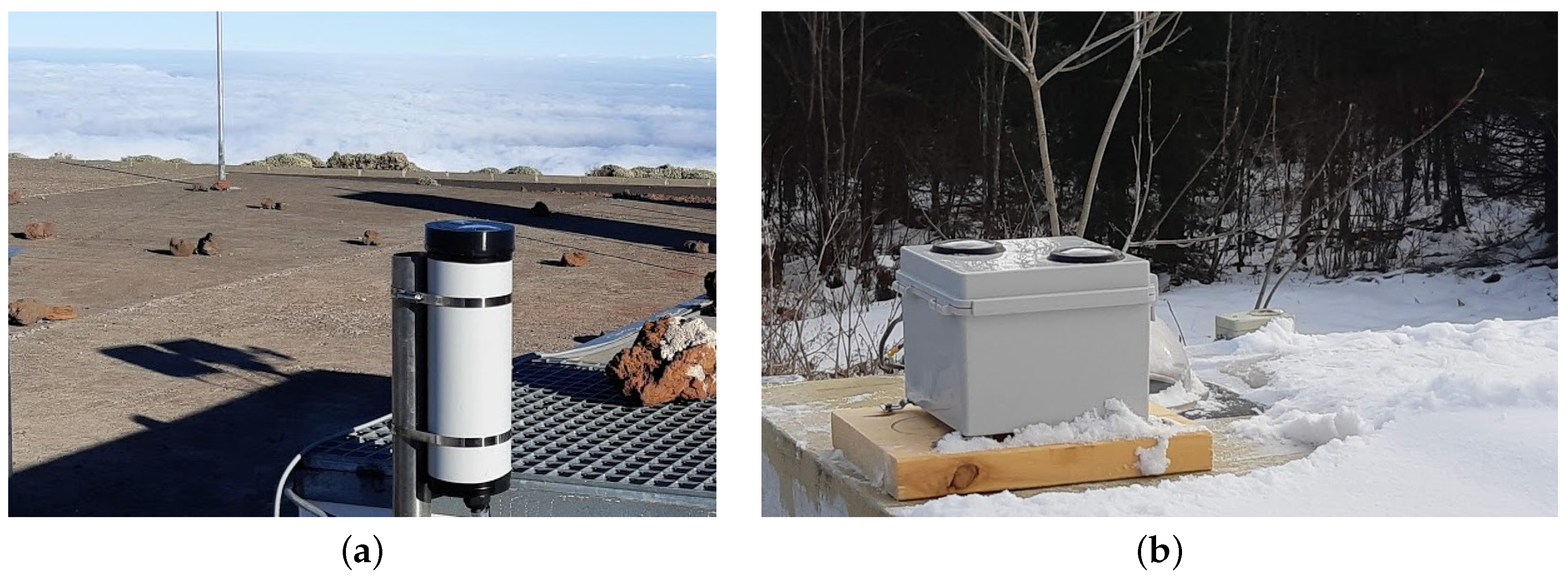
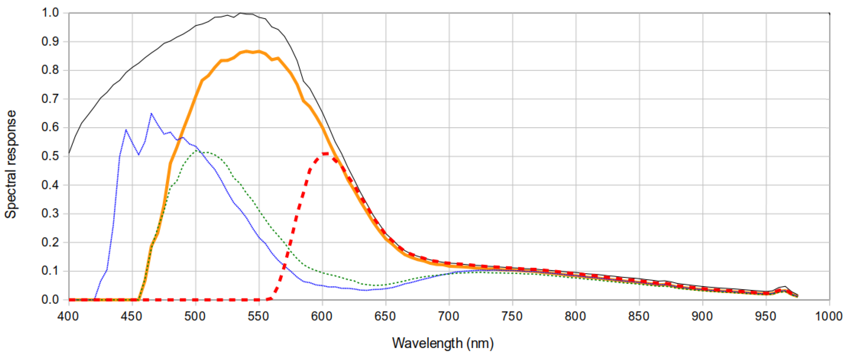
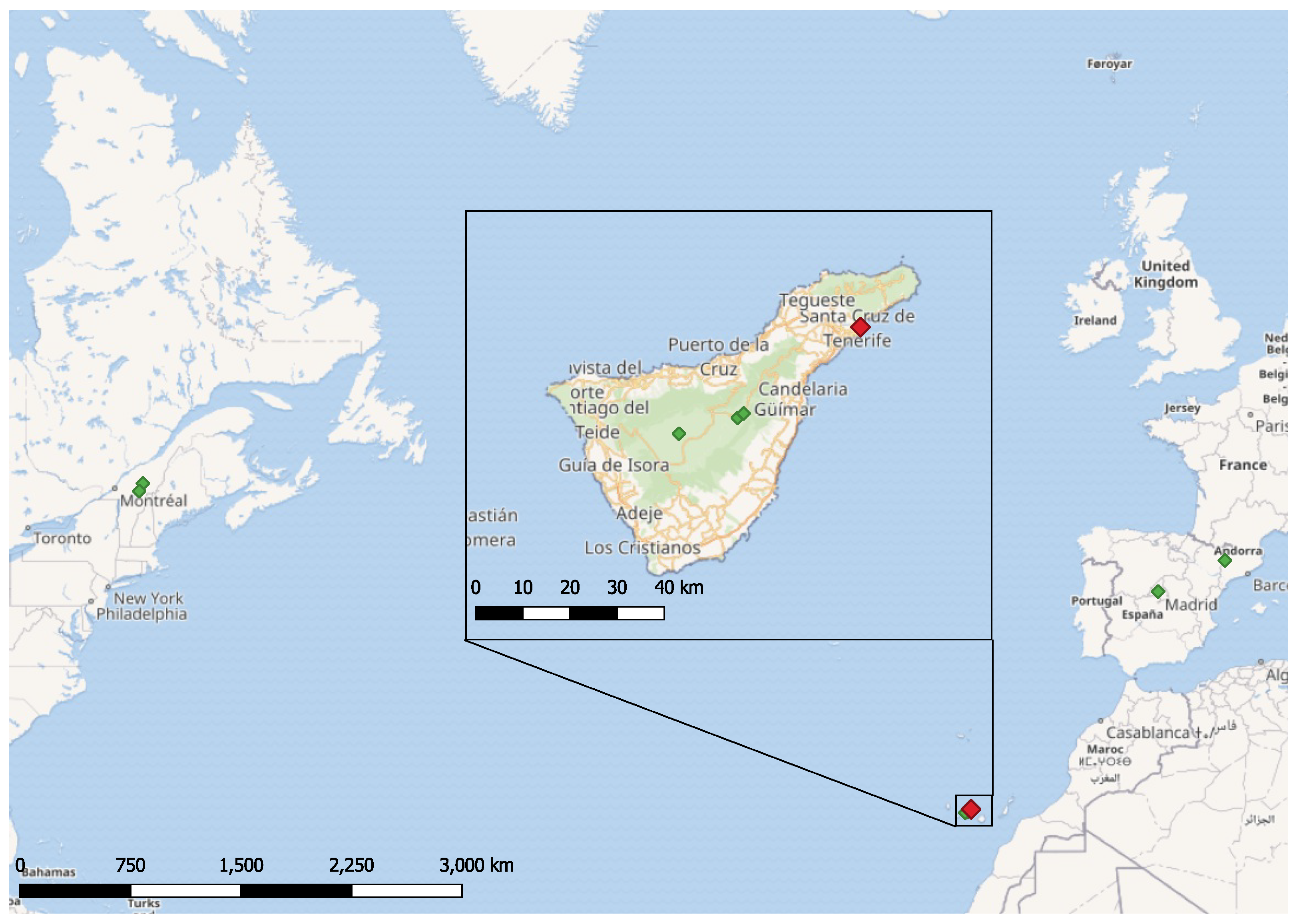
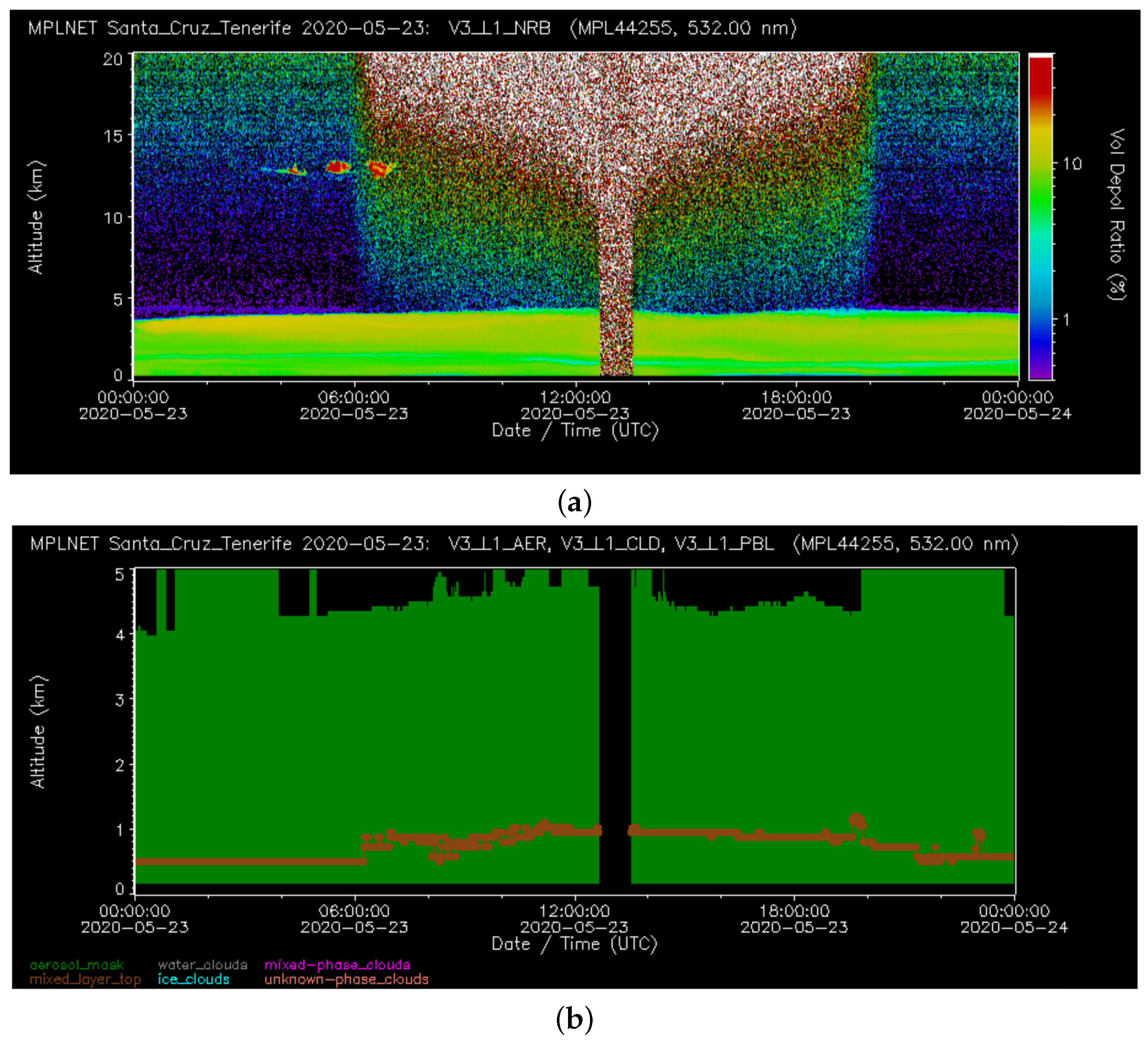
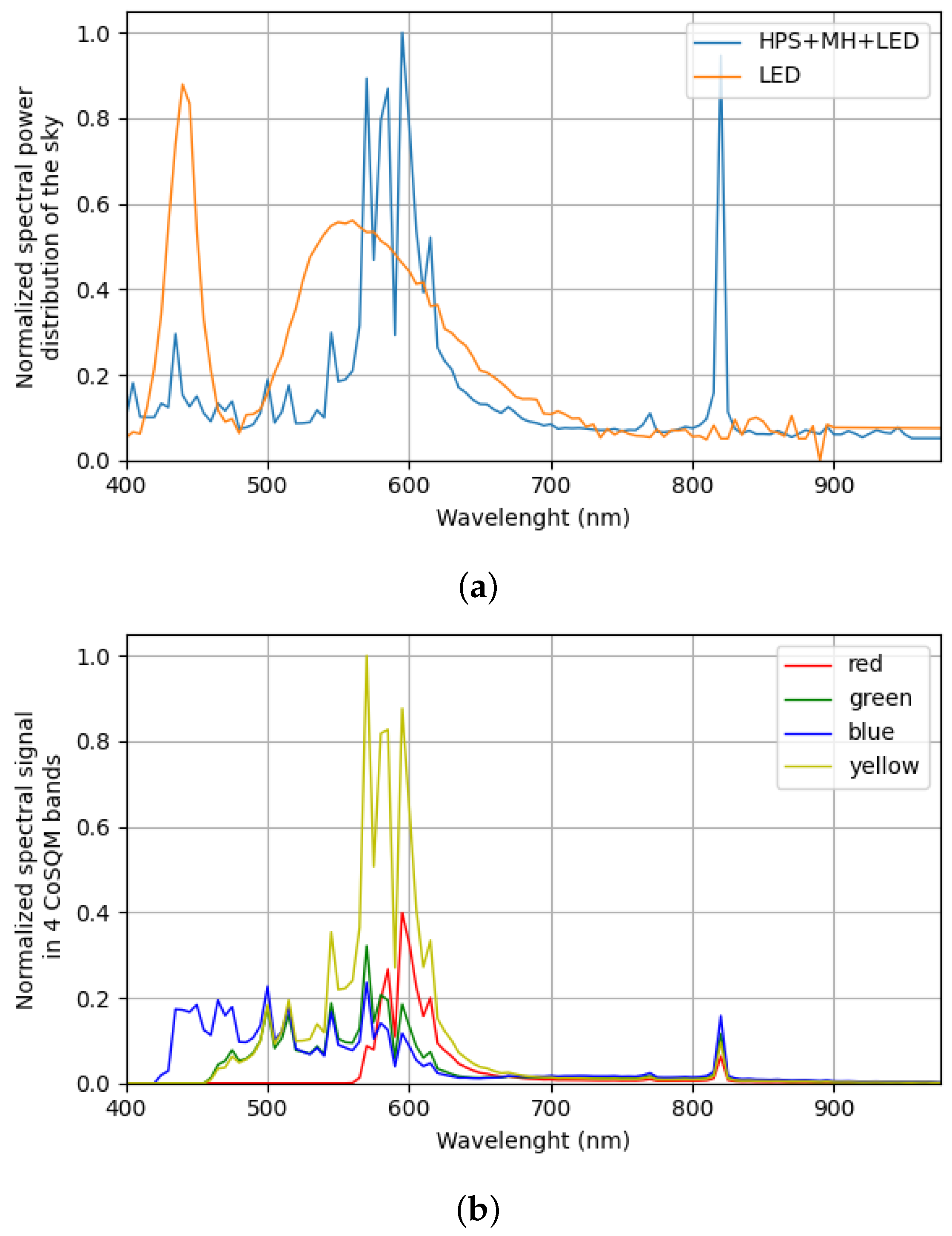
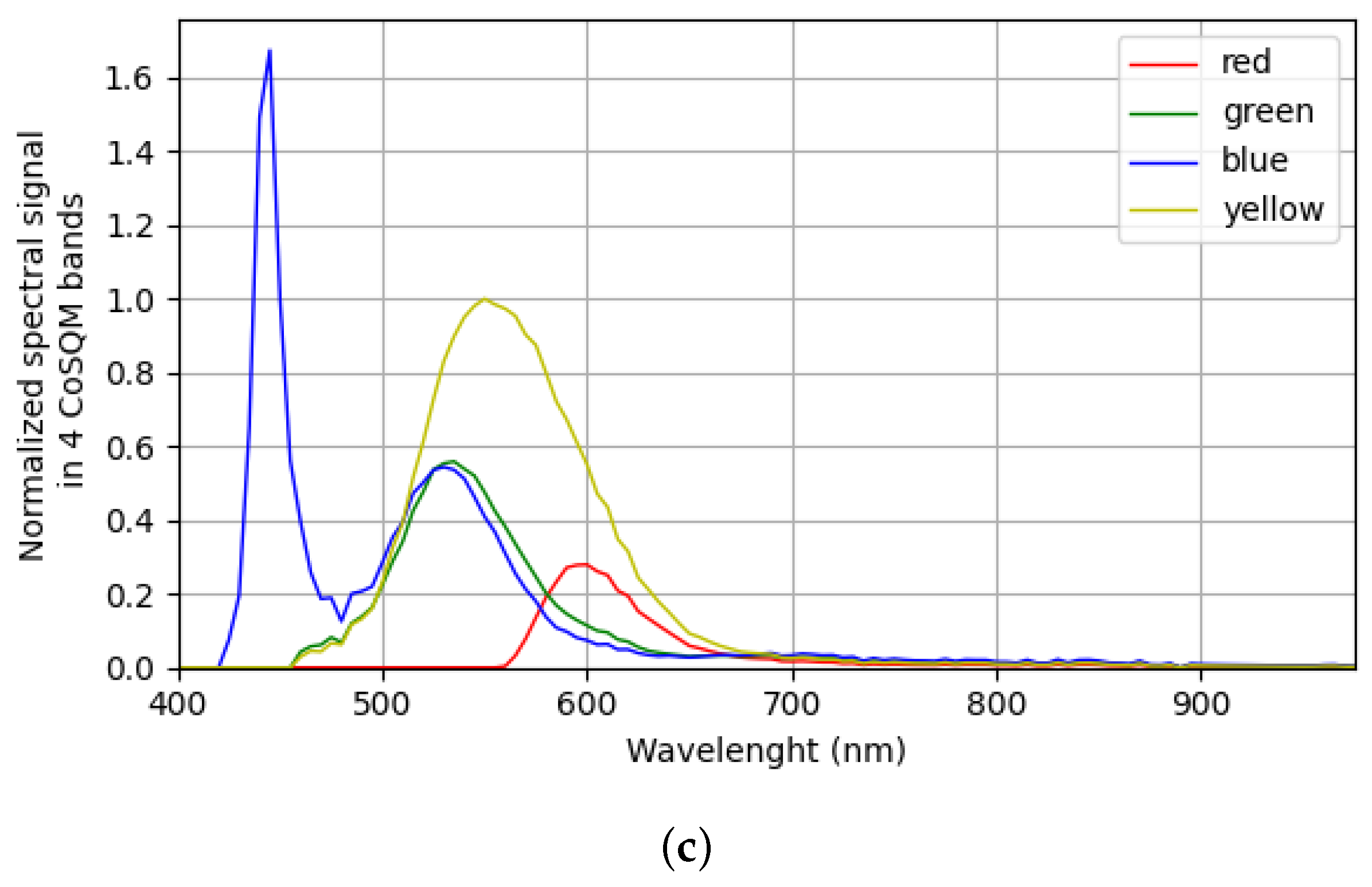
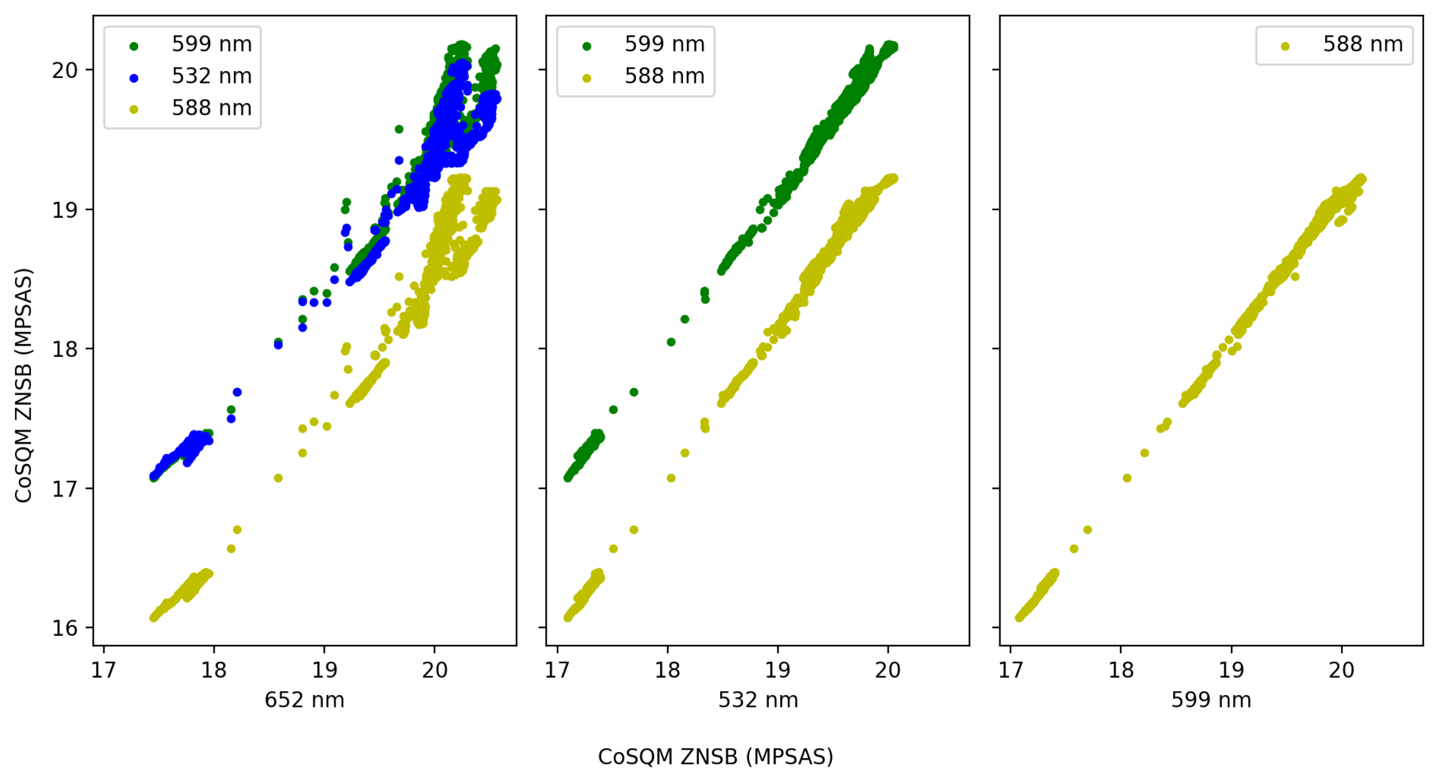

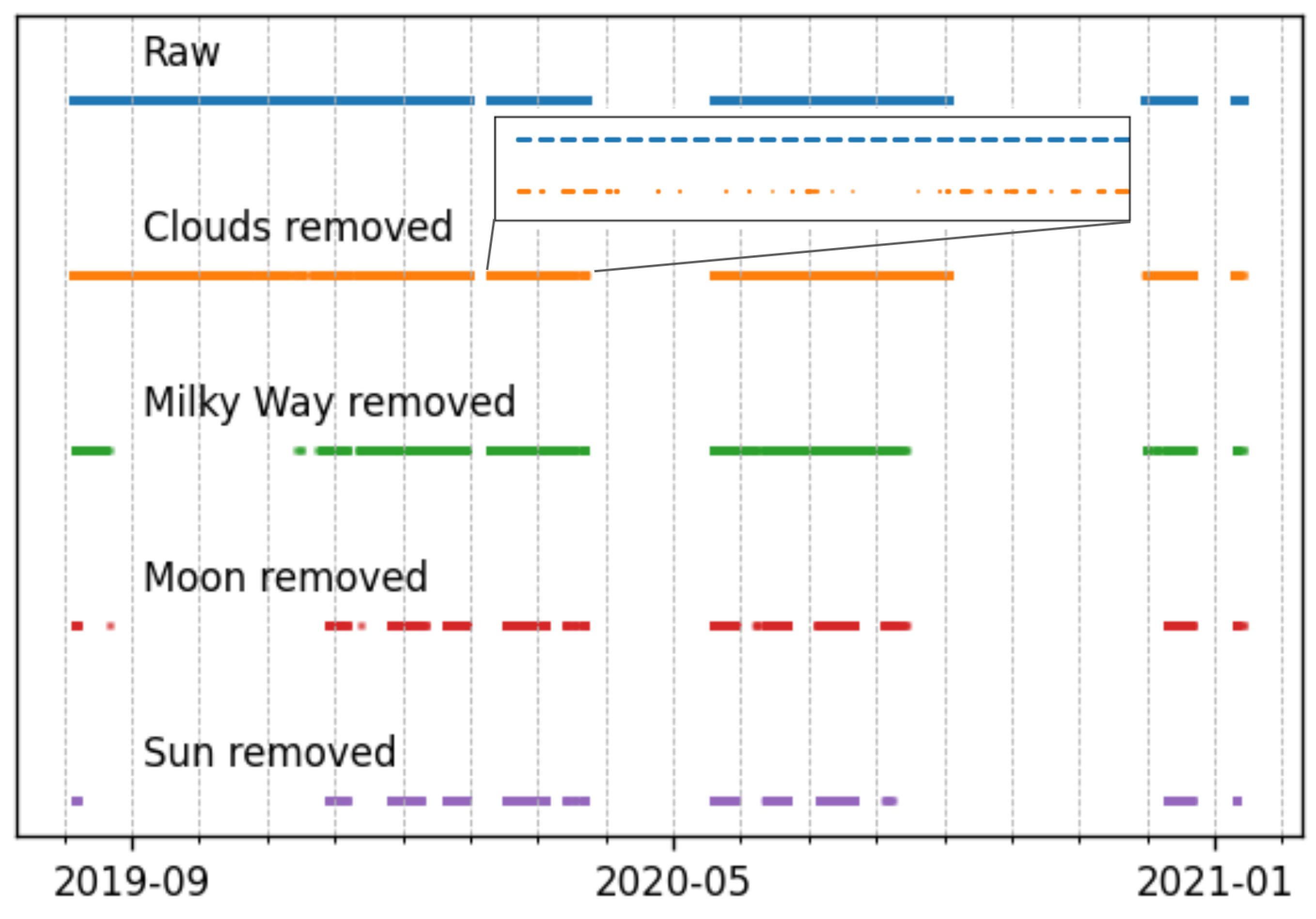
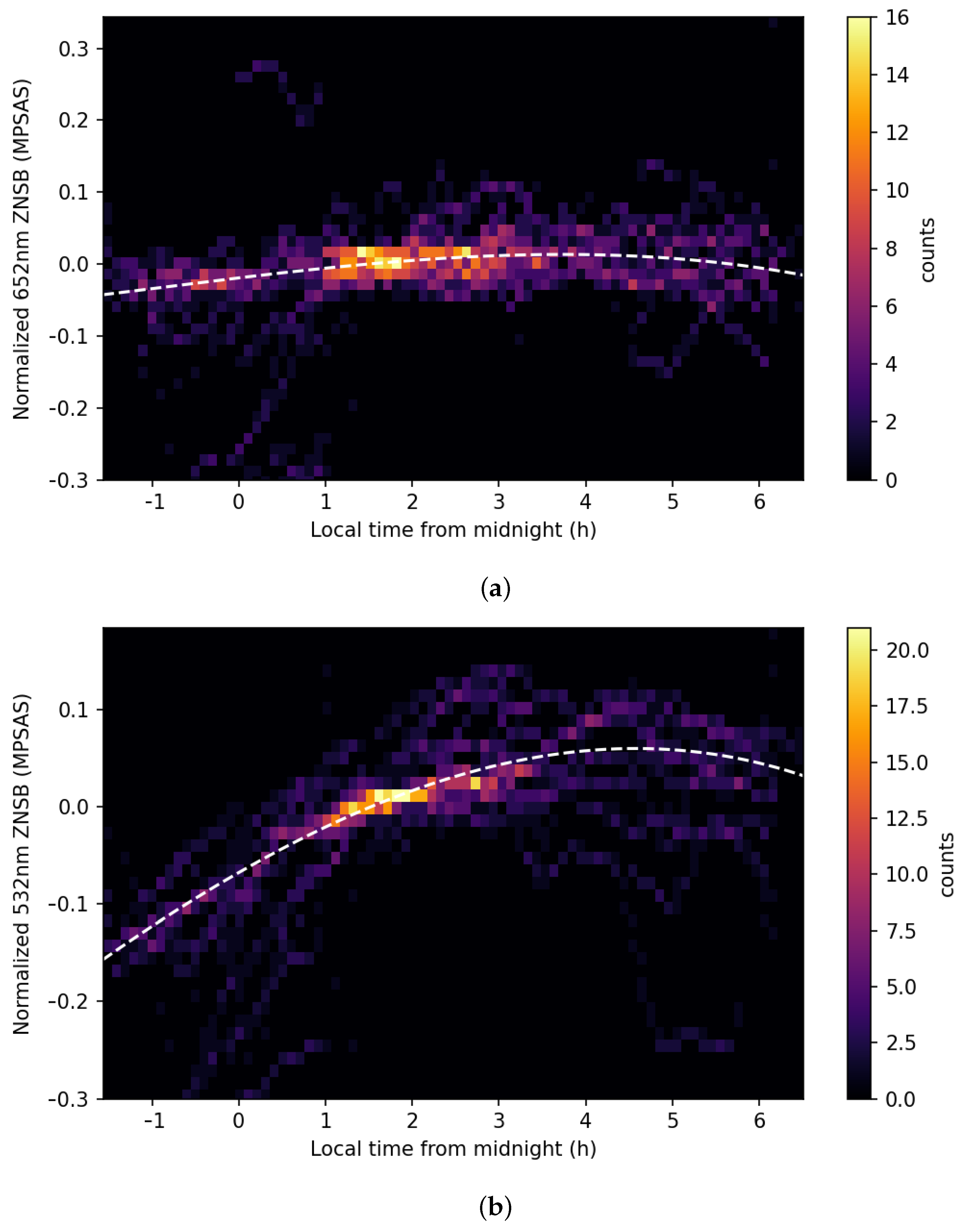
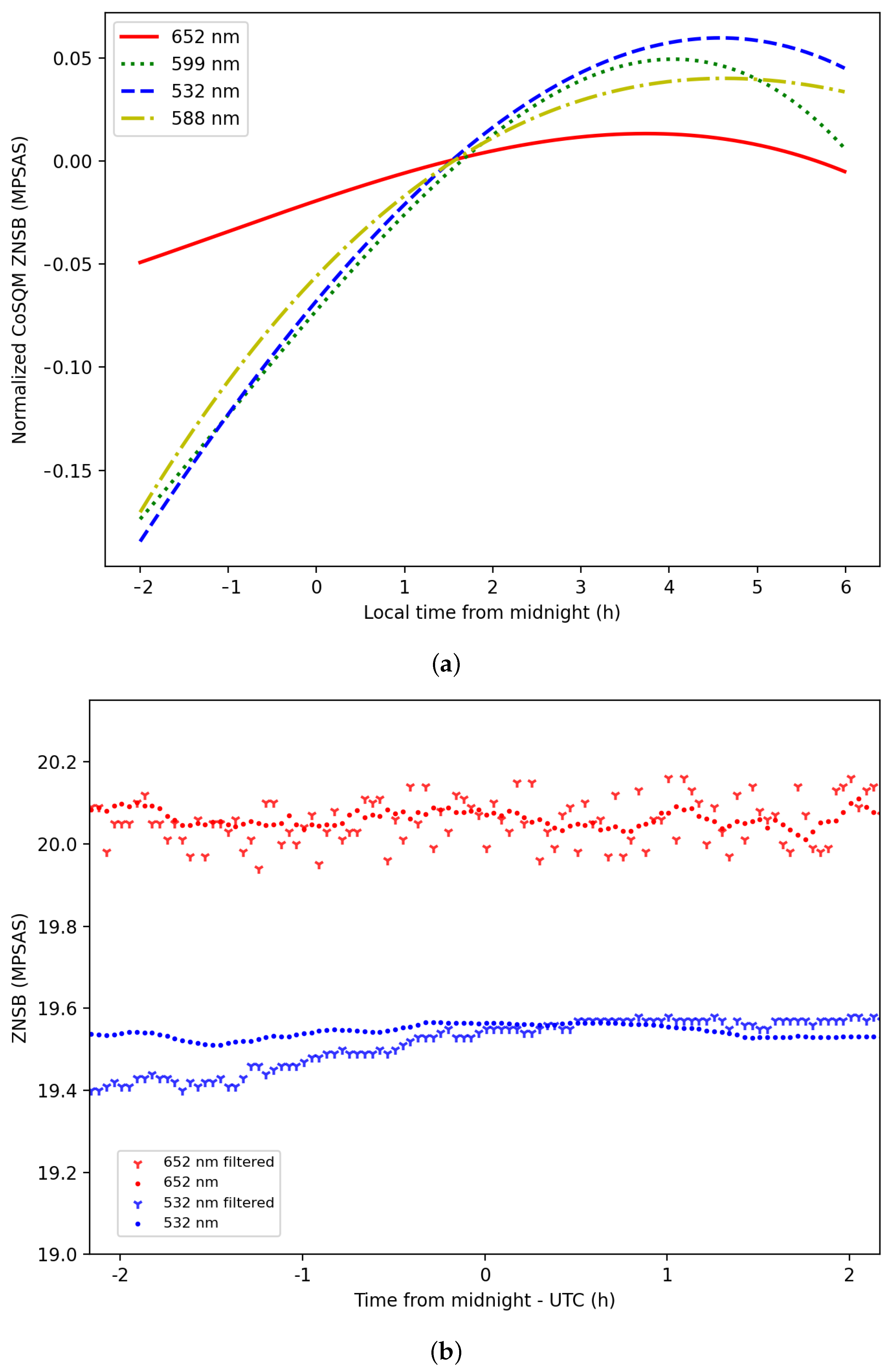
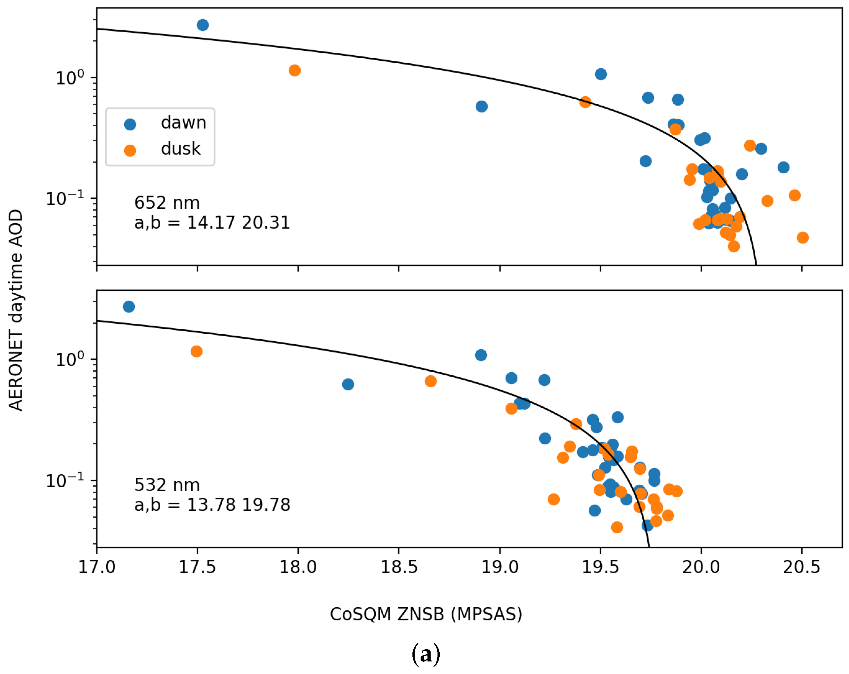
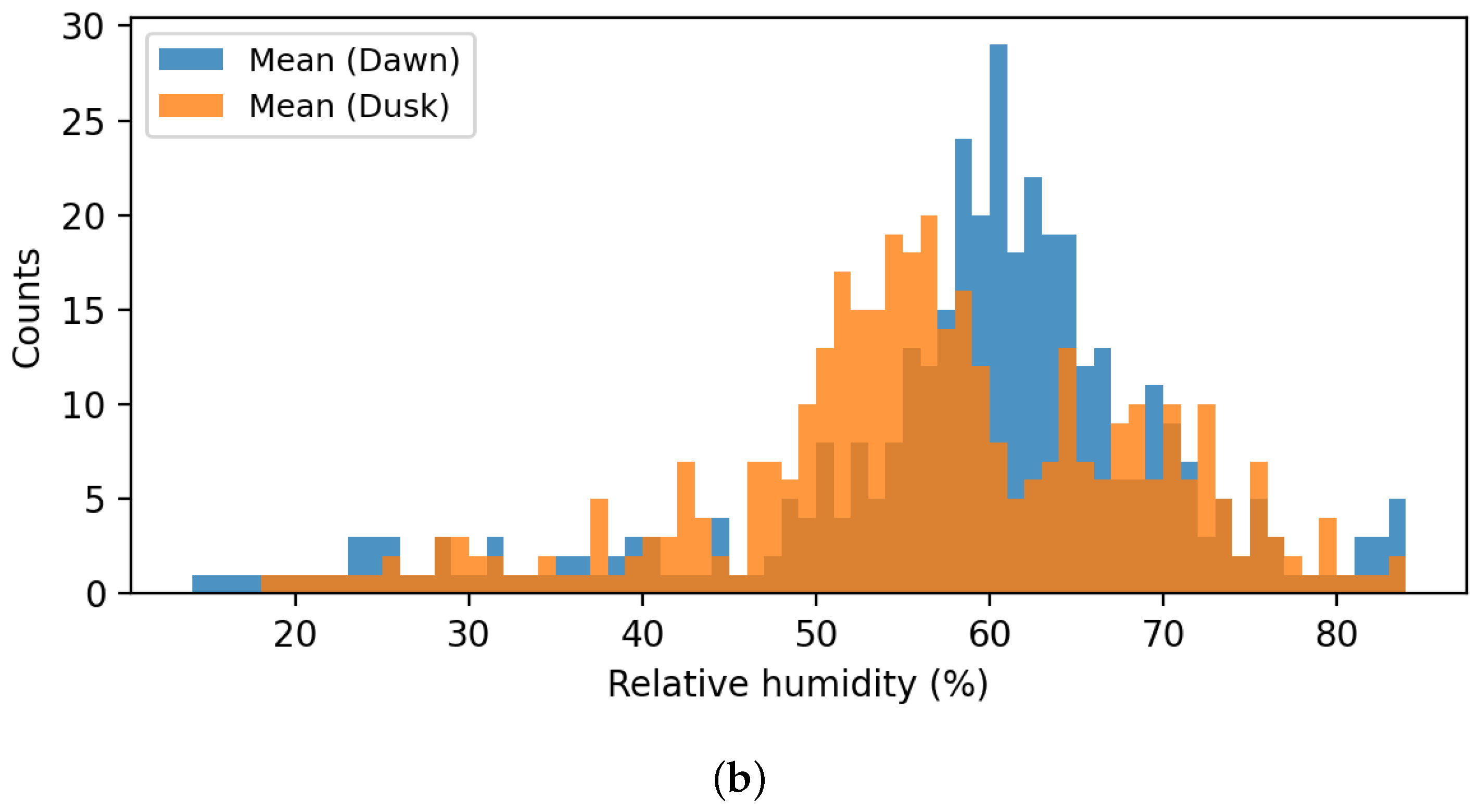
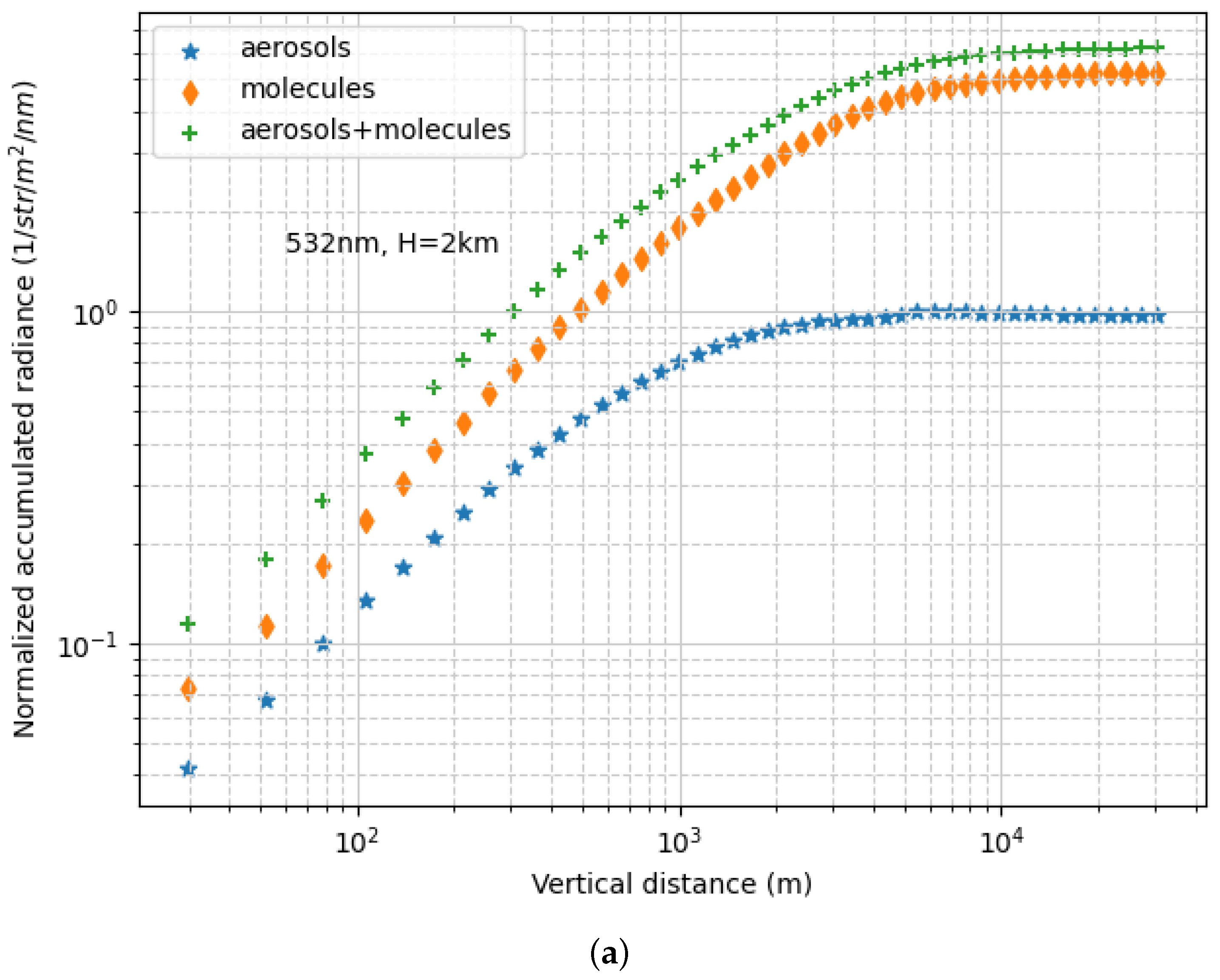
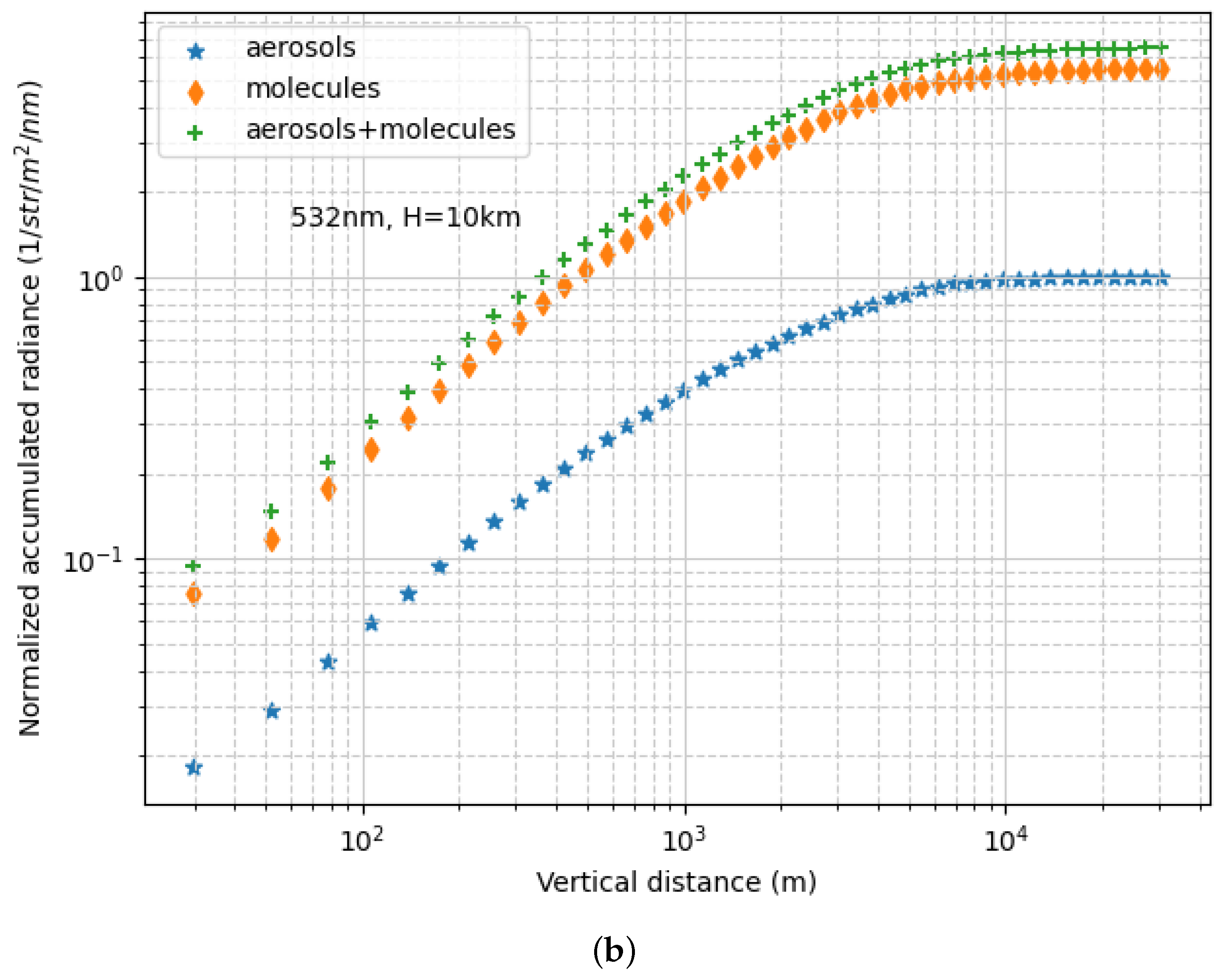
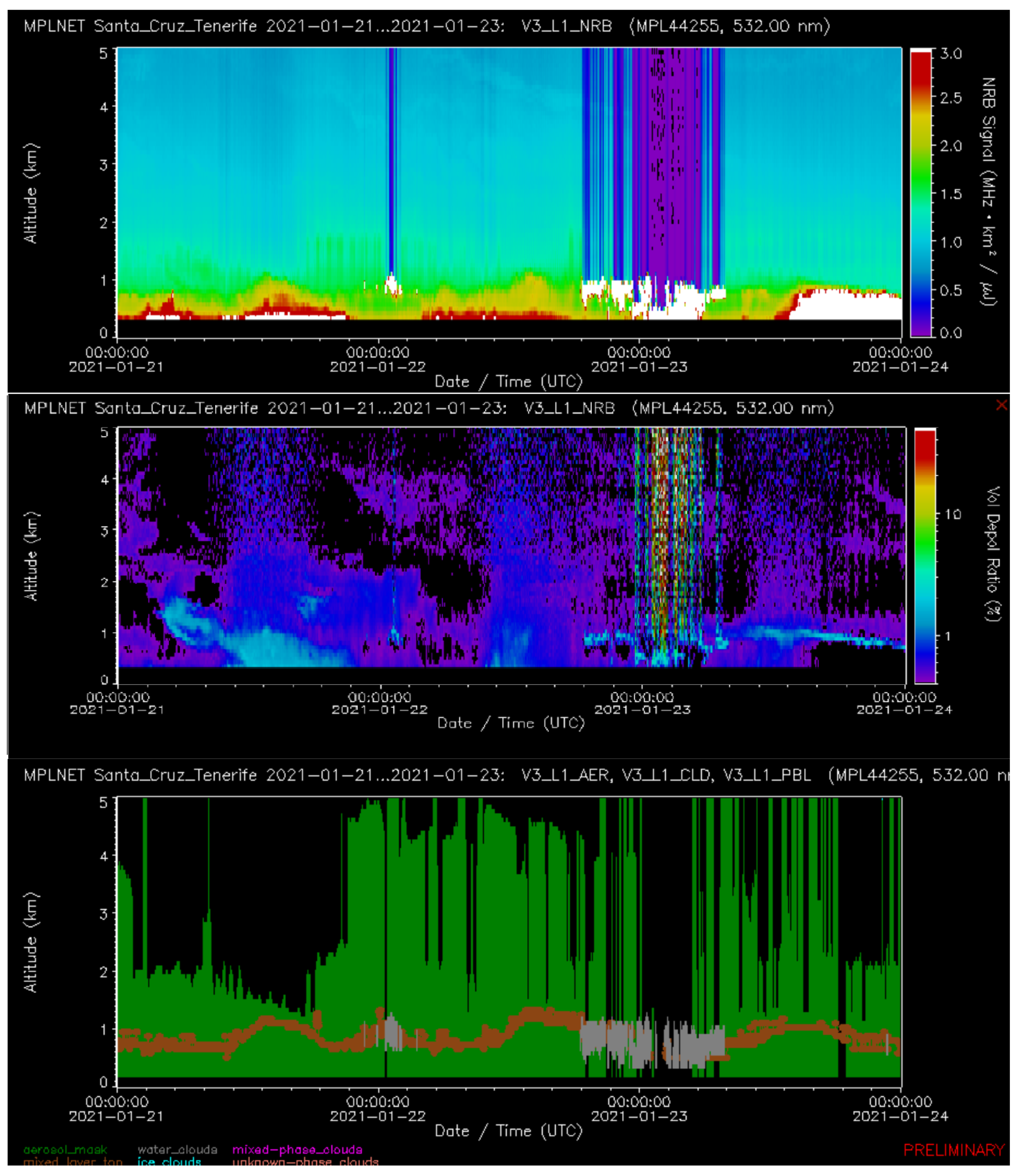
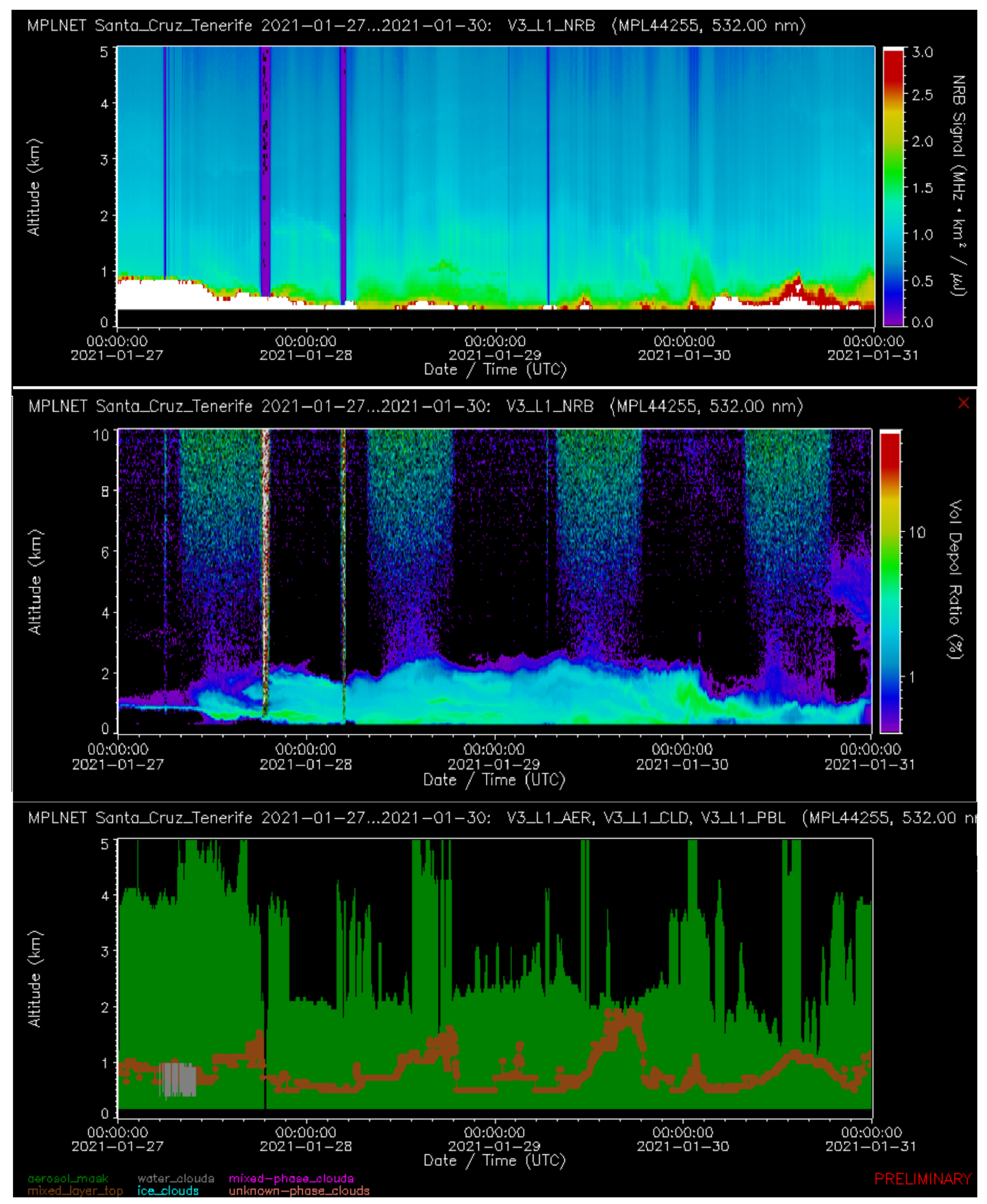
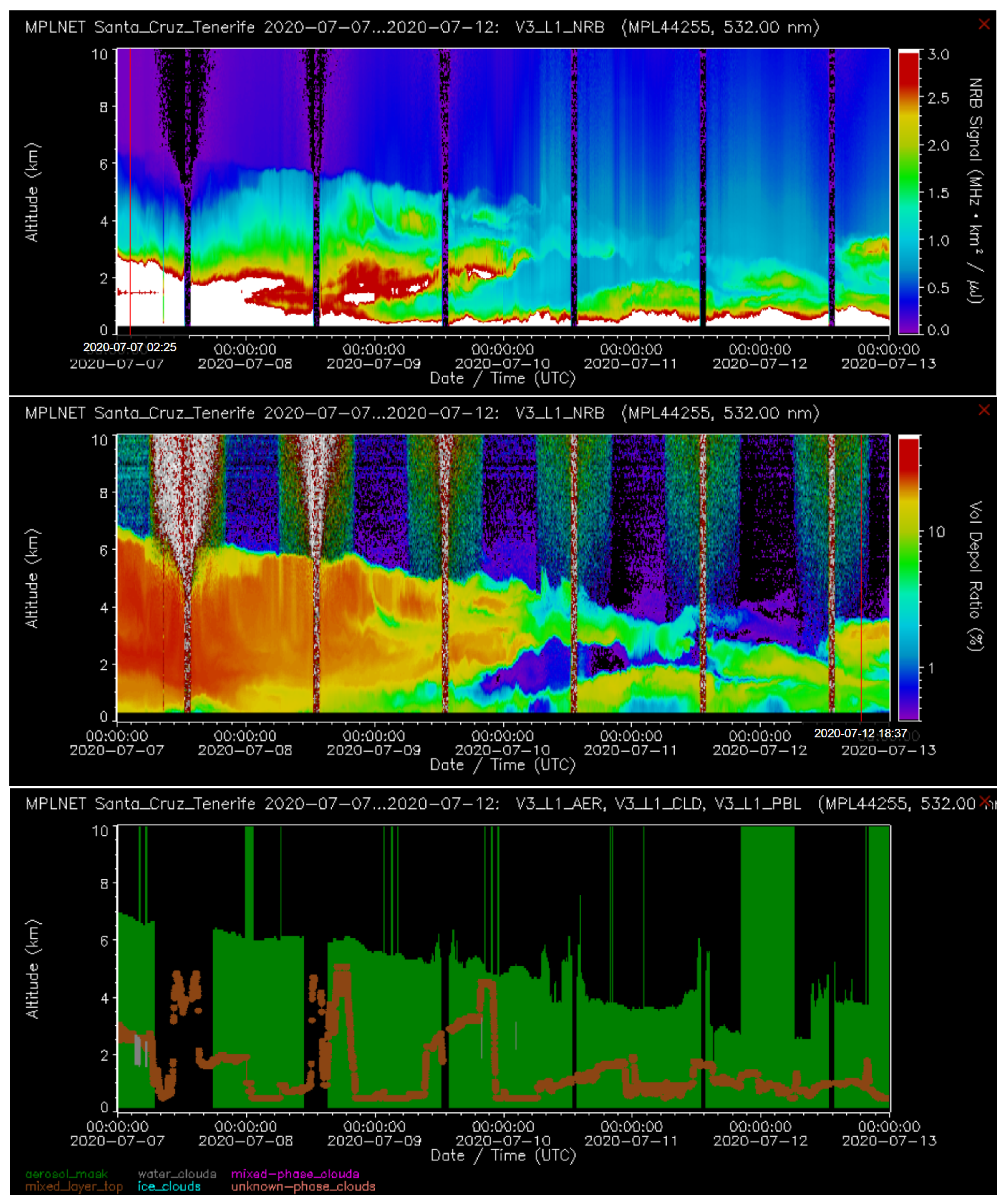
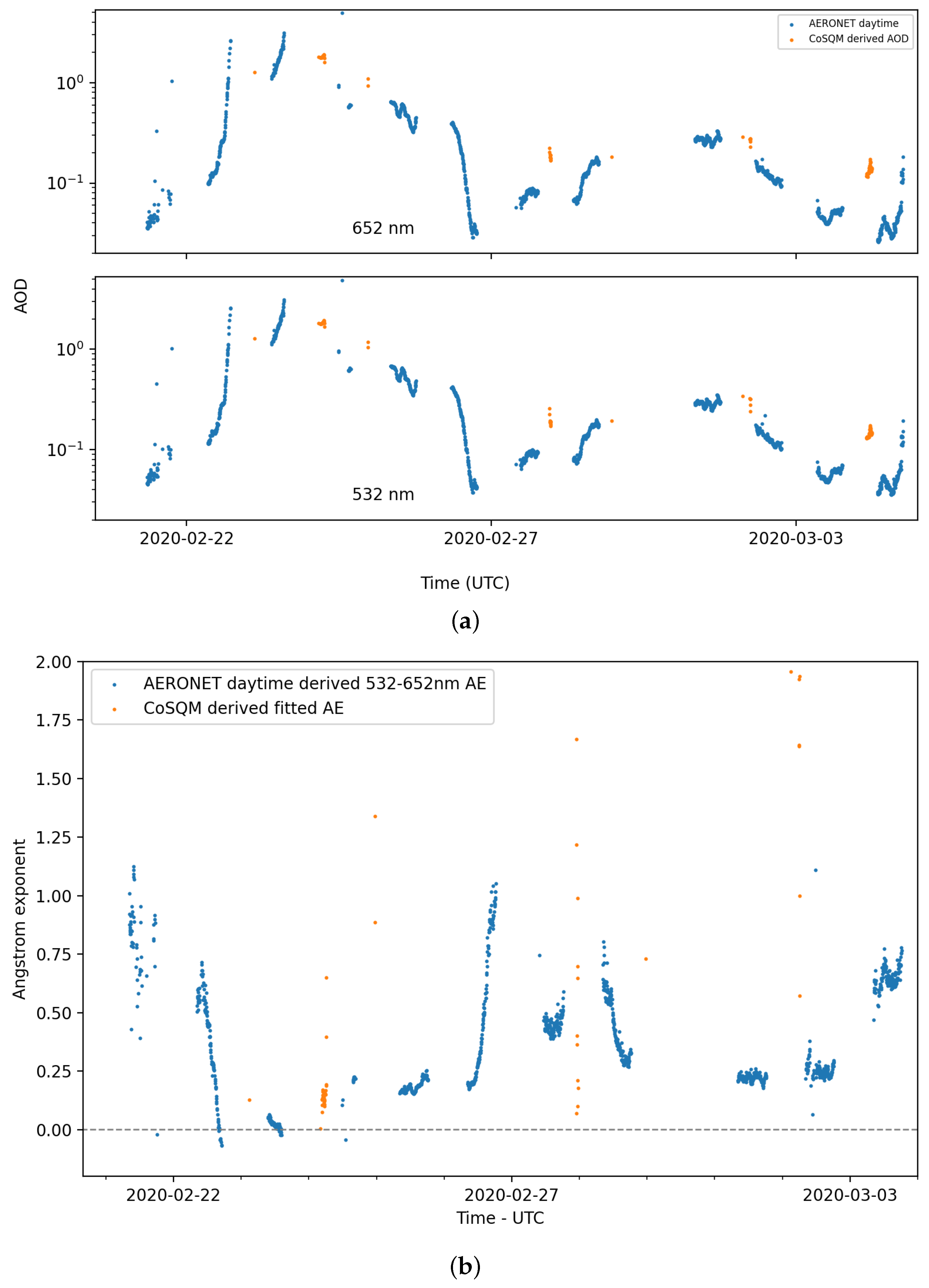
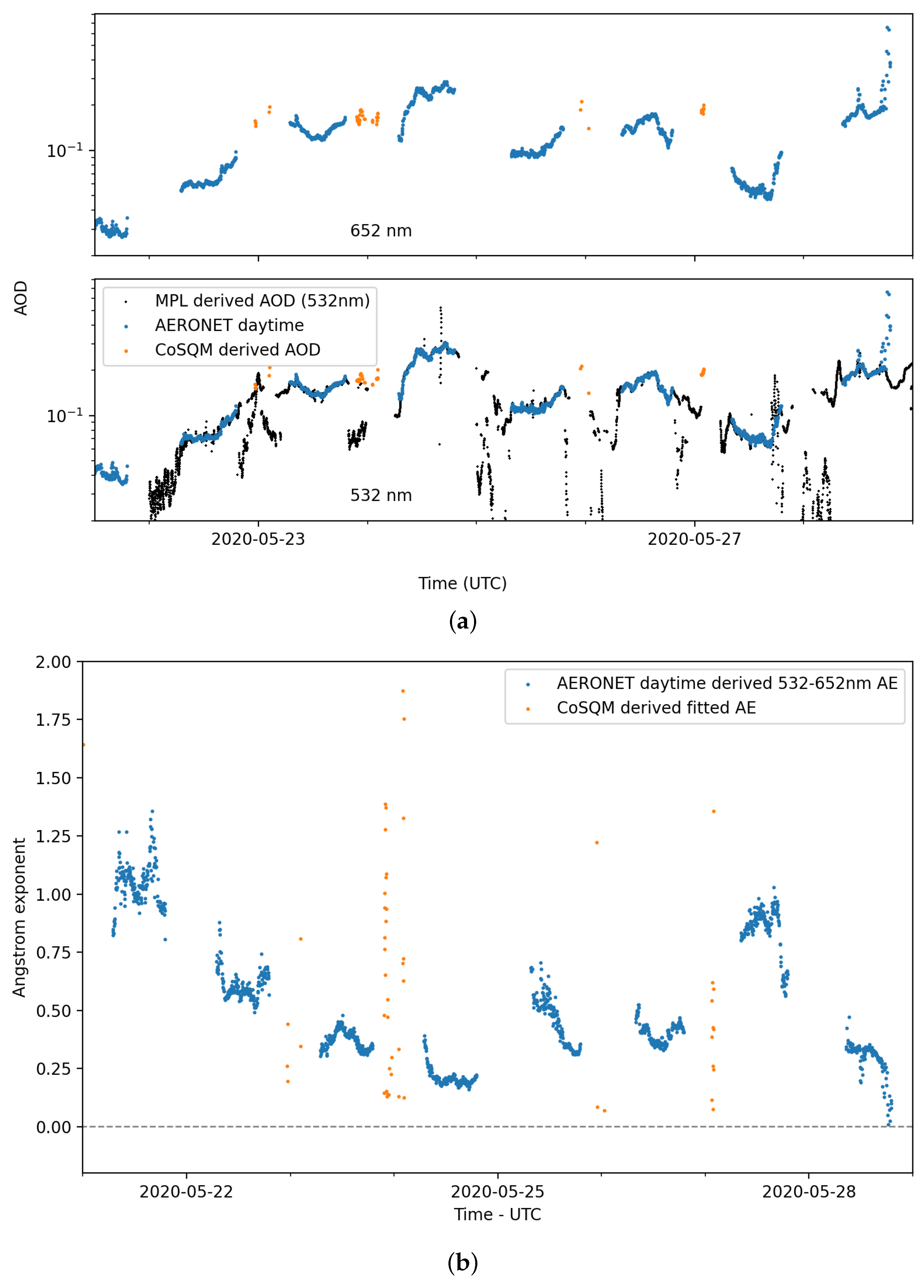
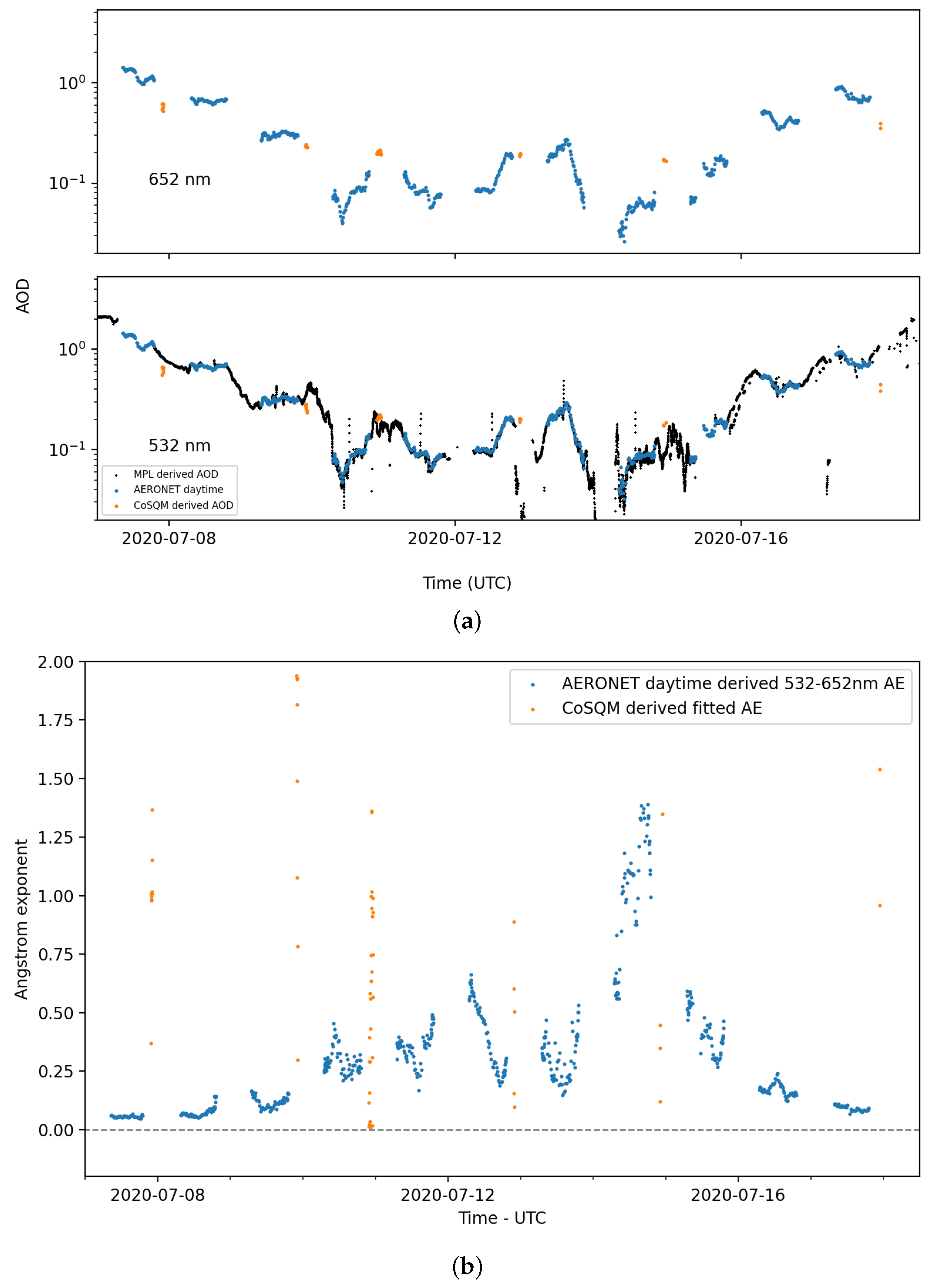
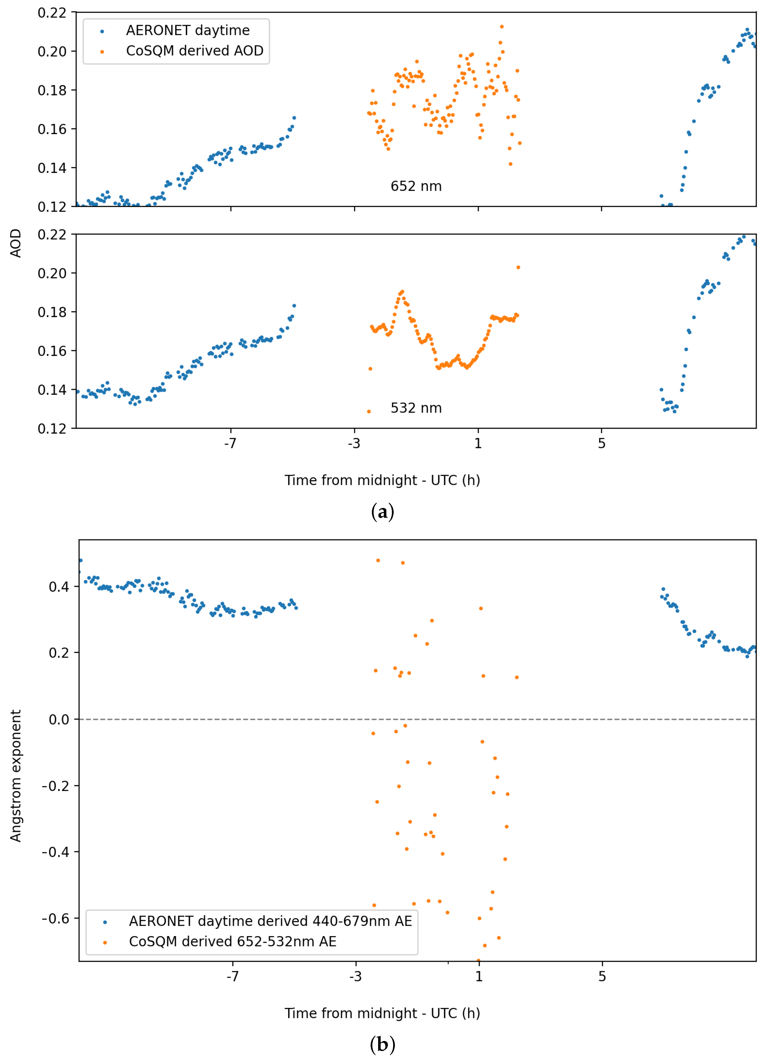

Publisher’s Note: MDPI stays neutral with regard to jurisdictional claims in published maps and institutional affiliations. |
© 2021 by the authors. Licensee MDPI, Basel, Switzerland. This article is an open access article distributed under the terms and conditions of the Creative Commons Attribution (CC BY) license (https://creativecommons.org/licenses/by/4.0/).