
A Novel 2D-3D CNN with Spectral-Spatial Multi-Scale Feature Fusion for Hyperspectral Image Classification

 ,
,  ,
,  and
and 
Abstract
:
1. Introduction
- (1)
- We propose a novel 2D-3D CNN with spectral-spatial multi-scale feature fusion for HSI classification, containing two feature extraction streams, a feature fusion module as well as a classification scheme. It can extract more sufficient and detailed spectral, spatial and high-level spectral-spatial-semantic fusion features for HSI classification;
- (2)
- We design a new hierarchical feature extraction structure to adaptively extract multi-scale spectral features, which is effective at emphasizing important spectral features and suppress useless spectral features;
- (3)
- We construct an innovative multi-level spatial feature fusion module with spatial attention to acquire multi-level spatial features, simultaneously, put more emphasis on the informative areas in the spatial features;
- (4)
- To make full use of both the spectral features and the multi-level spatial features, a multi-scale spectral-spatial-semantic feature fusion module is presented to adaptively aggregate them, producing high-level spectral-spatial-semantic fusion features for classification;
- (5)
- We design a layer-specific regularization and smooth normalization classification scheme to replace the simple combination of two full connected layers, which automatically controls the fusion weights of spectral-spatial-semantic features and thus achieves more outstanding classification performance.
2. Related Work
2.1. Convolutional Neural Networks
2.2. Residual Network
2.3. L2 Regularization
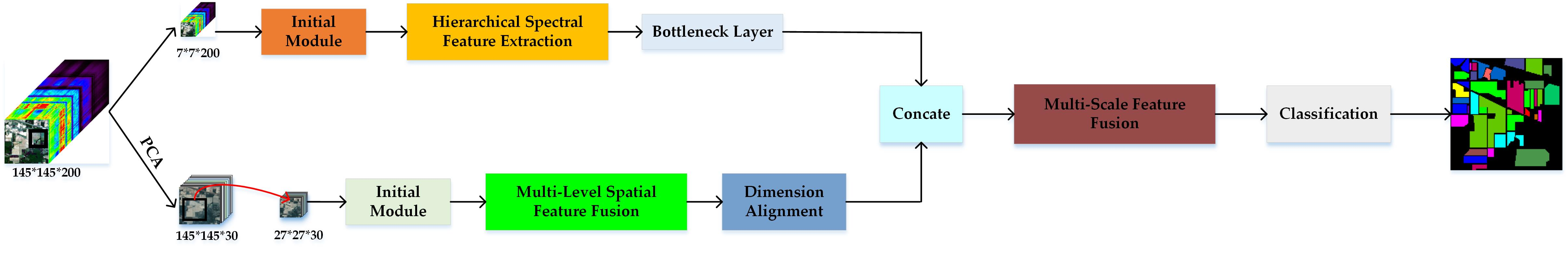
3. Proposed Method
3.1. The Spectral Feature Extraction Stream
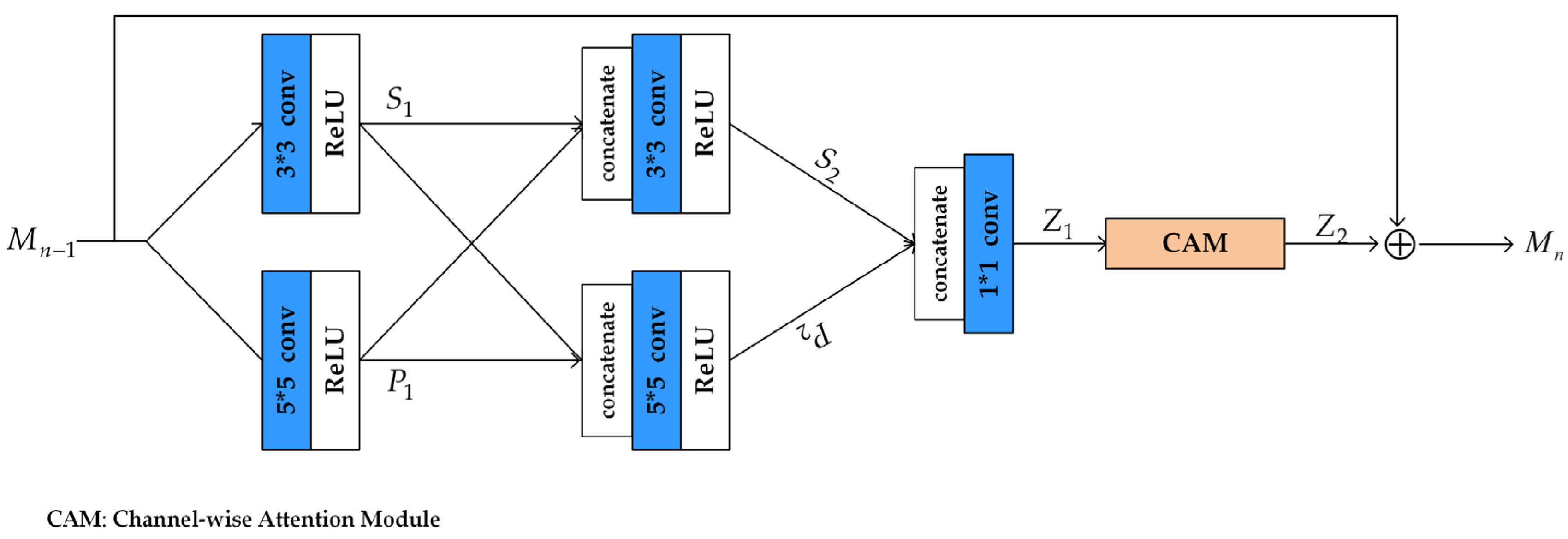
3.1.1. Hierarchical Spectral Feature Extraction Module
3.1.2. Hierarchical Feature Fusion Structure
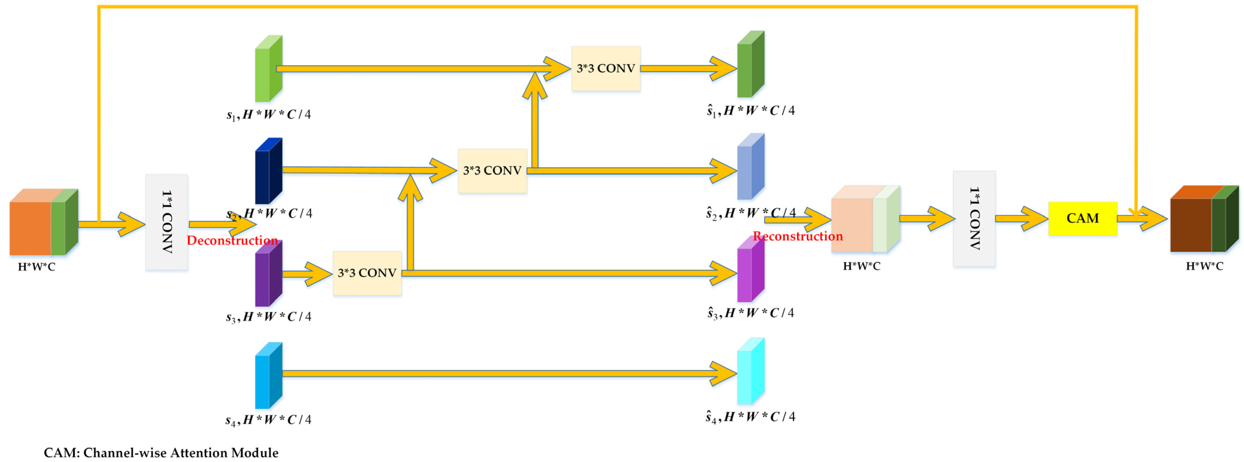
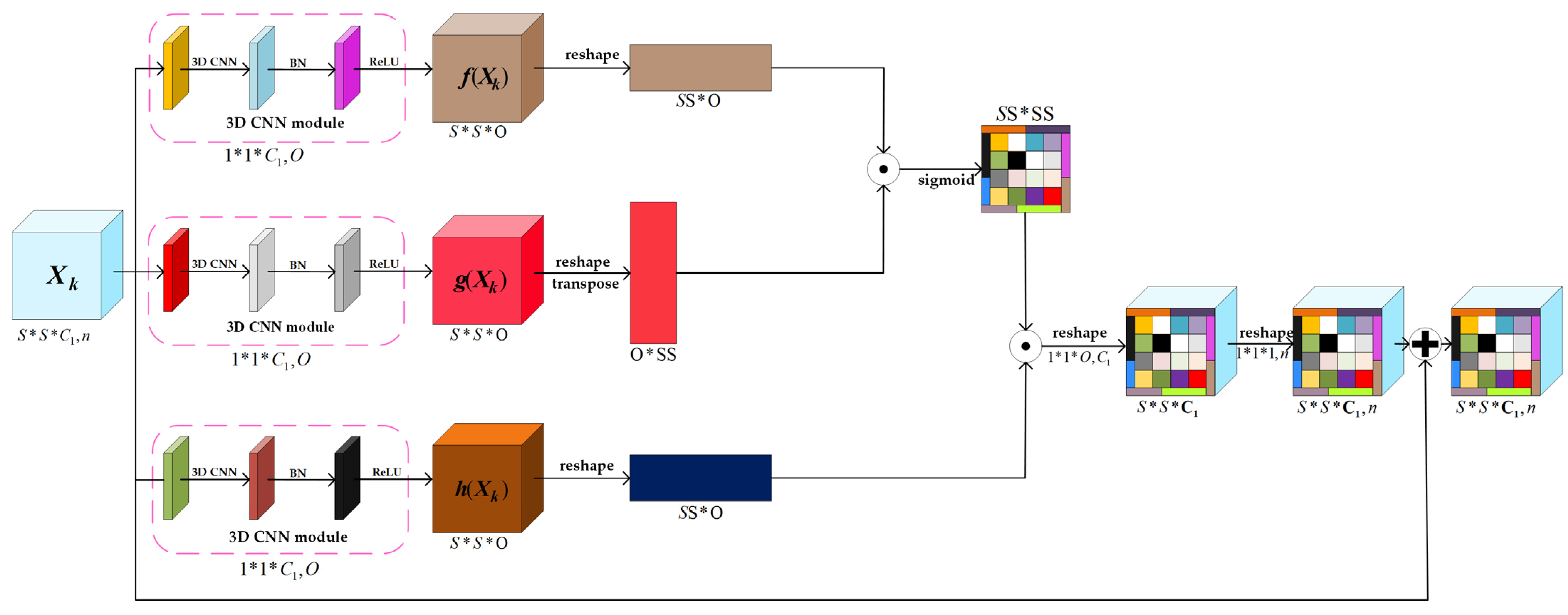
3.2. The Spatial Feature Extraction Stream
3.3. Multi-Scale Spectral-Spatial-Semantic Feature Fusion Module
3.4. Feature Classification Scheme
4. Experiments and Results
4.1. Experimental Datasets, Classification Evaluation Indexes and Experimental Setup
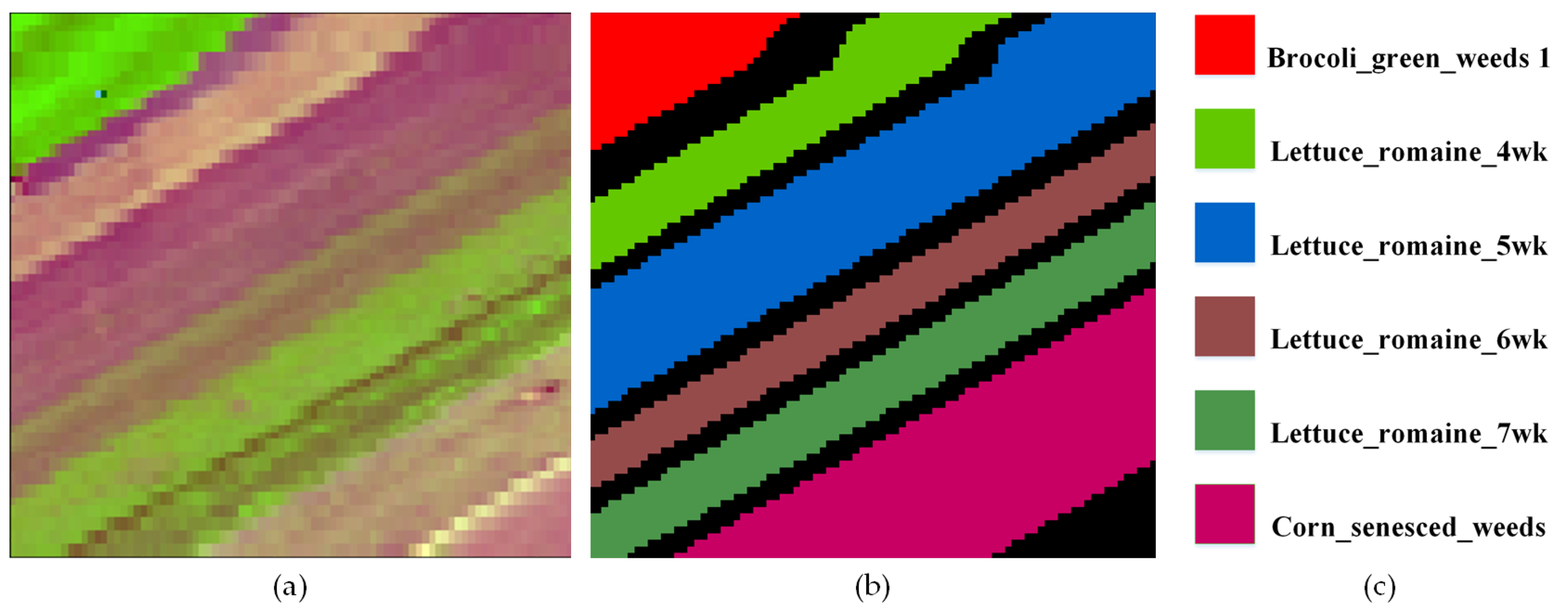
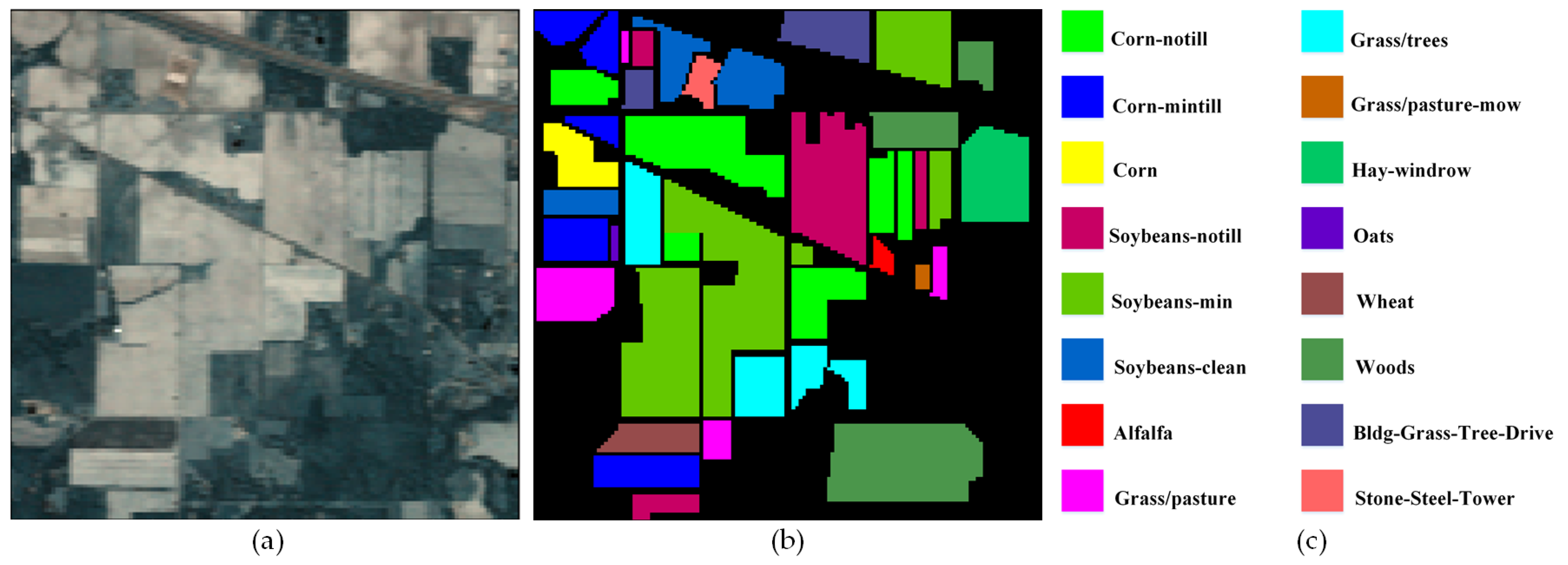
4.1.1. Experimental Datasets
4.1.2. Classification Evaluation Indexes
4.1.3. Experimental Setup
4.2. Experimental Parameters Discussion
4.2.1. Analysis of Different Ratios of the Training, Validation and Test Datasets
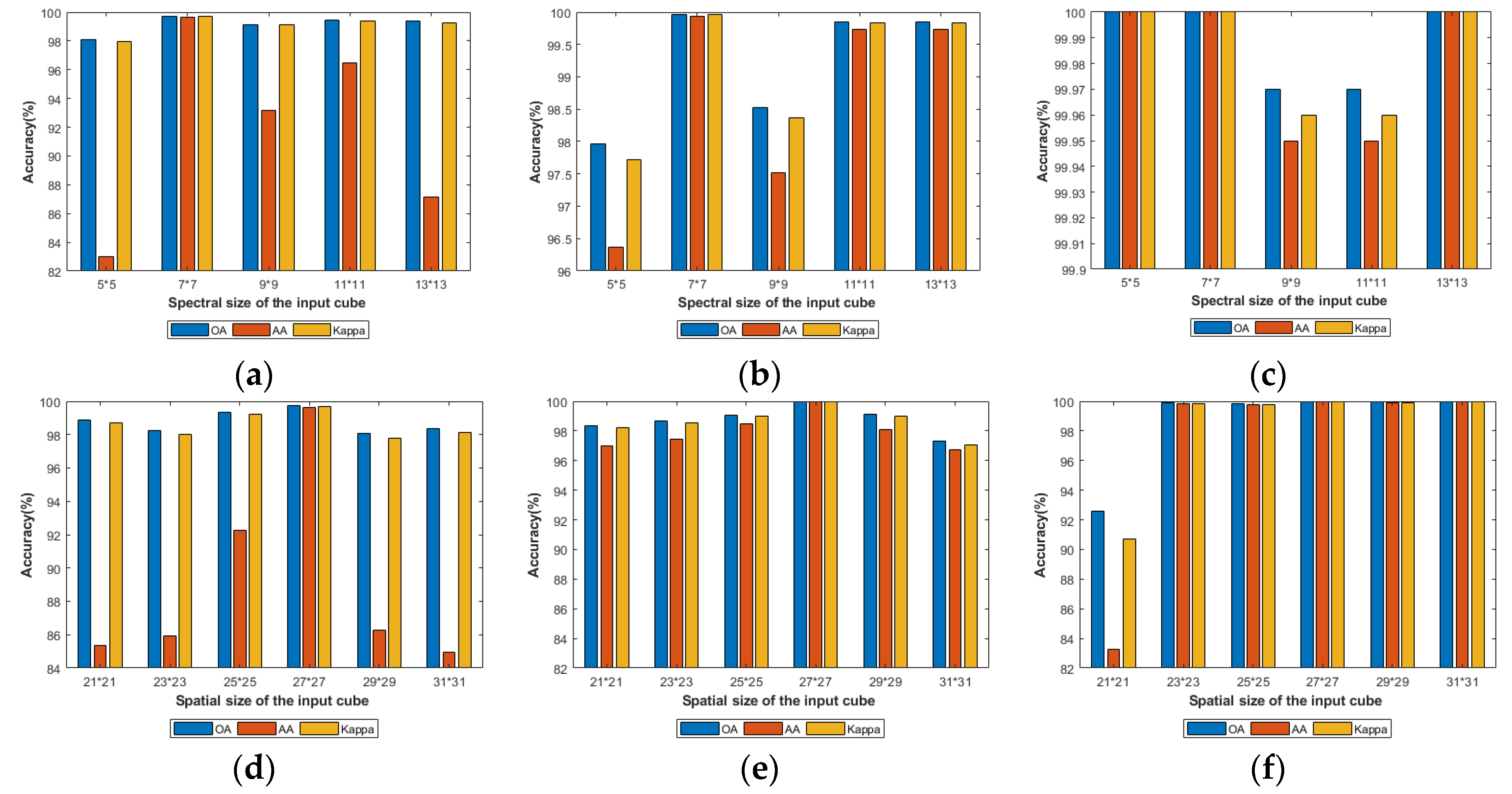
4.2.2. Analysis of the Patch Size
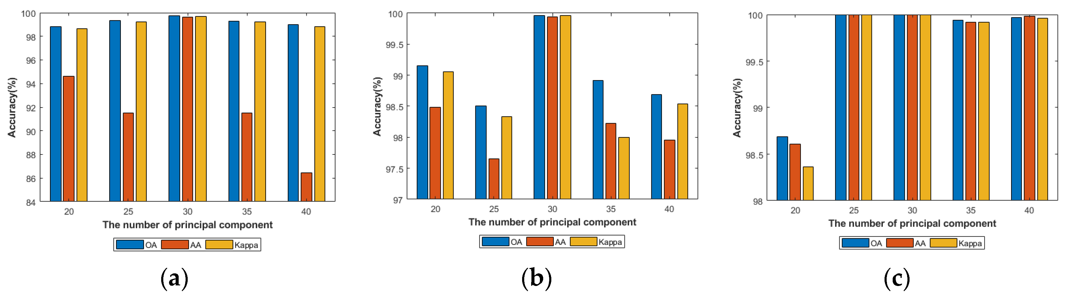
4.2.3. Analysis of the Principal Components of Spatial Feature Extraction Stream
4.2.4. Analysis of Different Ratios of Channel-Wise Attention Module
4.3. Classification Results Comparison with the State-of-the-Art Methods
- (1)
- From the tables, we can see clearly that compared with other methods, the proposed SMFFNet method has the highest evaluation indexes on three HSI datasets. Specifically, first, compared with three traditional classification methods, deep learning methods achieve generally higher evaluation indexes and better classification performance, except 2-D CNN and RSSAN on the IN data set, 2-D CNN on the KSC data set and 1-D CNN on the SA data set. Because the deep learning methods can automatically extract features from HSI data and have better robustness. Second, compared with classification methods using spectral and spatial information (such as 3D-CNN, HybridSN etc.), classification methods only using spectral information (such as SVM, MLR, RF and 1-D CNN) or spatial information (such as 2-D CNN) obtain lower classification accuracy and worse classification performance, except RSSAN on the IN dataset. It means that these classification methods cannot make full use of spectral and spatial information of HSI. Third, the proposed SMFFNet achieve the highest OA, AA and Kappa with a significant improvement over the above mentioned deep learning methods. For instance, in the Table 6, SMFFN method achieves OA 99.74% with the gains of 17.42%, 41.42%, 1.08%, 5.85%, 4.48%, 32.8% and 0.76% over 1-D CNN, 2-D CNN, 3-D CNN, Hybrid, JSSAN, RSSAN and TSCNN methods, respectively. The other two HSI datasets have semblable classification results. The complexity of 3-D CNN, Hybrid, JSSAN, RSSAN, TSCNN and SMFFNet methods is 0.001717184G, 0.01210803G, 0.000273436G, 0.000261567G, 0.00454323G and 0.010243319G, respectively. Furthermore, compared with these methods, our proposed SMFFNet can classify all categories on three datasets more accurately. It means that the proposed SMFFNet only need fewer training samples to get better classification performance and excellent evaluation indexes.
- (2)
- The TSCCN method consists of a local feature extraction stream and a global feature extraction stream. Nevertheless, our proposed SMFFNet method includes a spectral feature extraction stream, a spatial feature extraction stream and a multi-scale spectral-spatial-semantic feature fusion module. The TSCNN method and the proposed SMFFNet method employ a similar two-stream structure. From the tables, compared with the TSCNN method, the proposed SMFFNet method achieved the highest classification accuracy and a better classification performance. To be specific, on the IN dataset, the OA, AA and Kappa of the SMFFNet method are 0.76%, 5.85% and 3.86% higher than those of the TSCNN method respectively. Moreover, only two classes of our proposed method have lower classification accuracy than those of the TSCCN method. The other two HSI datasets have semblable classification results. This is because that the TSCNN method only uses several ordinary consecutive convolution operations embedded SE modules to extract shallow spectral and spatial features and ignores high-level semantic. However, our proposed SMFFNet not only extracts multi-scale spectral features and multi-level spatial features, but also maps the low-level spectral/spatial features to high-level spectral-spatial-semantic fusion features for improving HSI classification.
- (3)
- The Hybrid method is based on 2D-3D CNN for HSI classification. Nevertheless, our proposed SMFFNet method also employs 2D-3D CNN for HSI classification. The Hybrid method and the proposed SMFFNet method takes 2D-3D CNN as the basic framework. From the tables, compared with the Hybrid method, the evaluation indexes of the proposed SMFFNet method are higher than those of it. Specifically, the OA, AA and Kappa of the SMFFNet method are 5.85%, 5.86% and 5.67% higher than those of the Hybrid method on the IN dataset, respectively. Moreover, only one class of our proposed method has lower classification accuracy than that of the Hybrid method. The other two HSI datasets have semblable classification results. Although the Hybrid method uses 2D-3D convolution to extract spectral and spatial features, it does not extract coarse spectral-spatial fusion features and ignores the close correlation between spectral and spatial information.
- (4)
- The JSSAN, RSSAN, TSCCN and our proposed SMFFNet methods embed an attention mechanism to enhance feature extraction ability. From the tables, we can see that the OA, AA, Kappa and the classification accuracy of each category of our SMFFNet method are the highest. It means that we use channel-wise attention mechanism and spatial attention mechanism to improve the feature extraction capacity, enhance useful feature information and suppress unnecessary ones. These show that the proposed method combined with the attention mechanism can achieve a better classification performance and an excellent classification accuracy.
- (5)
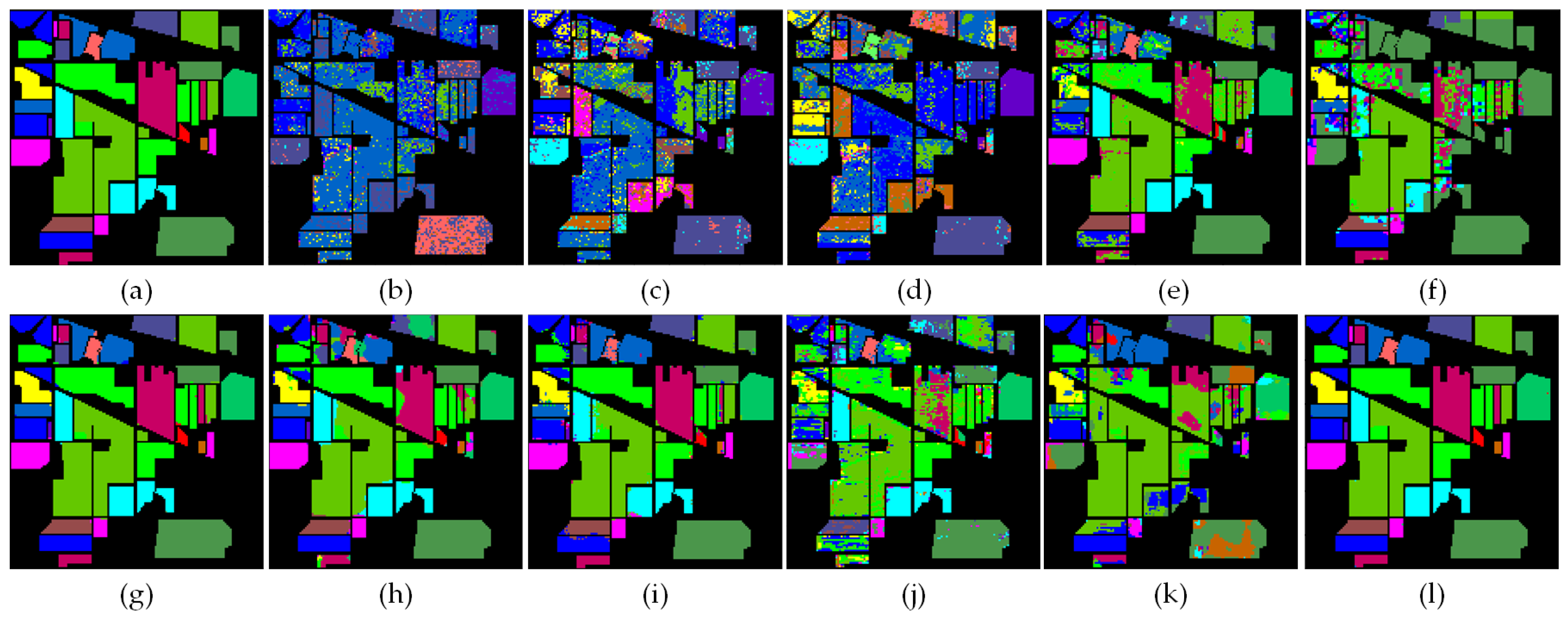
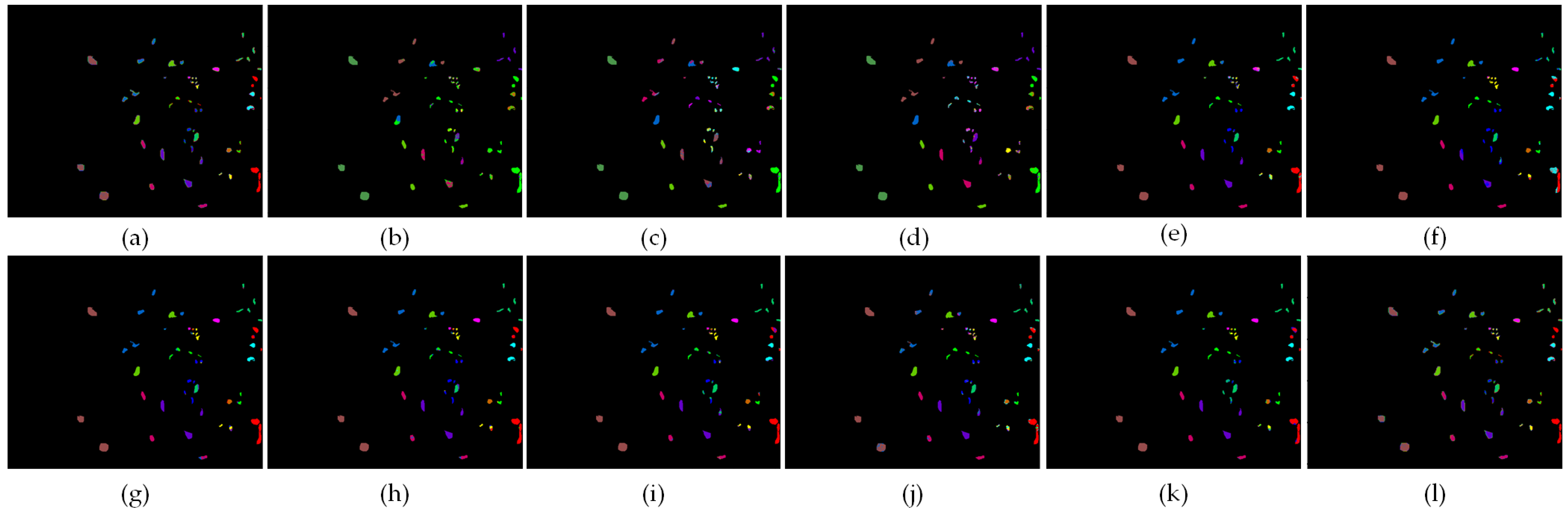
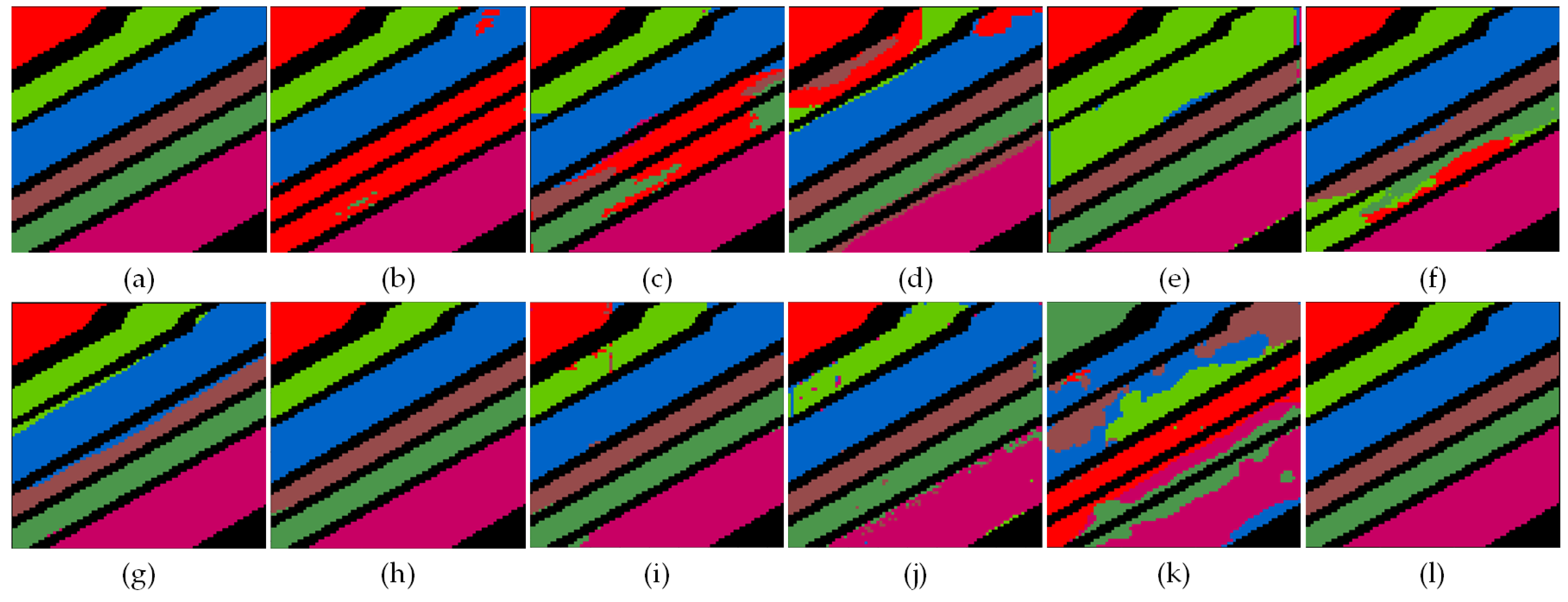
- Figure 13, Figure 14 and Figure 15 show the visualization maps of all categories of all classification methods, along with corresponding ground-truth maps. From the figures, we can find that the classification maps of SVM, MLR, RF, 1-D CNN, 2-D CNN, 3-D CNN, Hybrid, JSSAN, RSSAN and TSCNN have some dot noises in some categories. Compared with these classification methods, the proposed SMFFNet method has smoother classification maps. In addition, the edge of each category is clearer than others and the prediction effect on unlabeled samples is also significantly better, which indicates that the attention mechanism can effectively suppress the distraction of interfering samples. Compared with the proposed SMFFNet method, other methods cause the misclassification of many categories and their classification maps are very rough. Our proposed method not only has fairly smooth classification maps and more higher classification prediction accuracy. Owing to the idiosyncratic structure of SMFFNet method, it can fully extract the spectral-spatial-semantic features of the HSI and achieve more detailed and discriminable fusion features.
4.4. Ablation Experiments
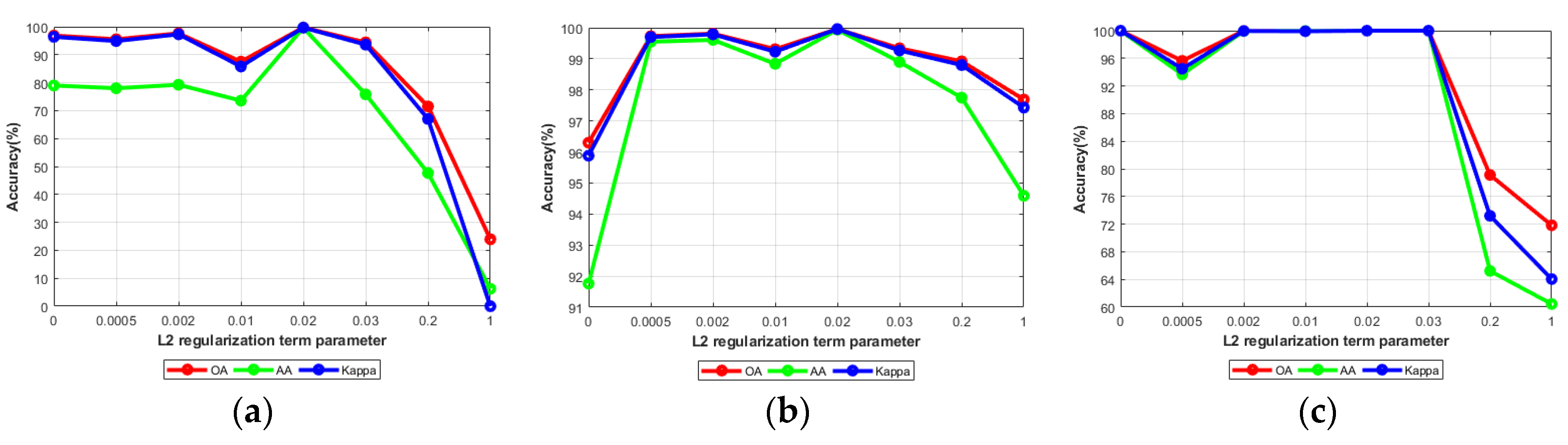
4.4.1. Analysis of Classification Scheme and L2 Regularization Parameter
4.4.2. Analysis of Attention Module
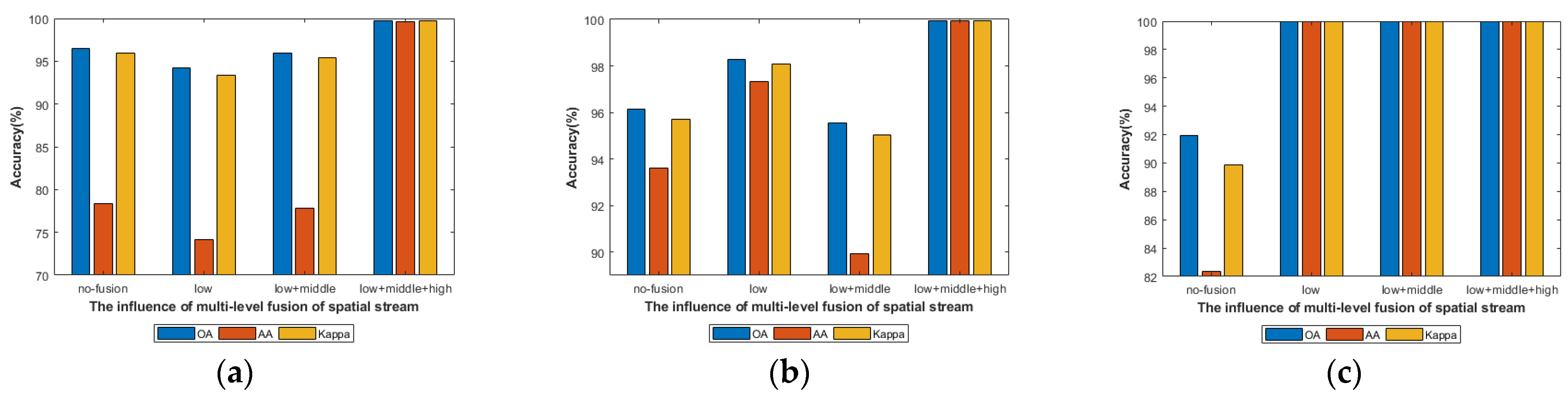
4.4.3. Analysis of Spectral, Spatial and Spectral-Spatial-Semantic Feature Stream
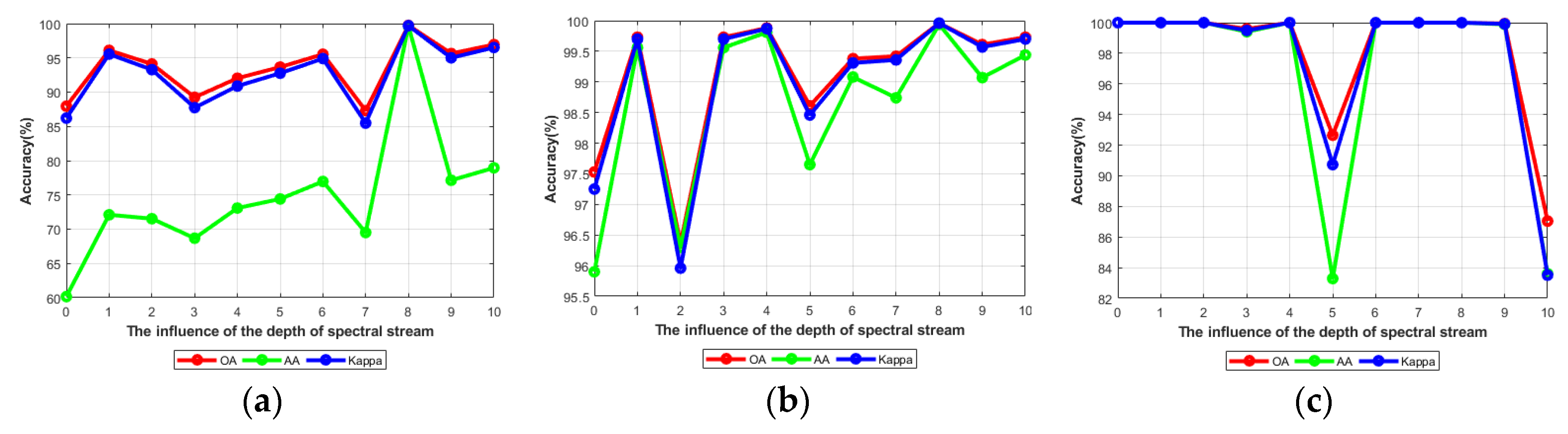
4.4.4. Analysis of the Network Depth
5. Discussion and Conclusions
Author Contributions
Funding
Data Availability Statement
Acknowledgments
Conflicts of Interest
References
- Landgrebe, D. Hyperspectral image data analysis. IEEE Signal Process. Mag. 2002, 19, 17–28. [Google Scholar] [CrossRef]
- Paoletti, M.E.; Haut, J.M.; Plaza, J.; Plaza, A. Deep learning classifiers for hyperspectral imaging: A review. ISPRS J. Photogramm. Remote Sens. 2019, 158, 279–317. [Google Scholar] [CrossRef]
- Zhu, L.; Chen, Y.; Ghamisi, P.; Benediktsson, J.A. Generative Adversarial Networks for Hyperspectral Image Classification. IEEE Trans. Geosci. Remote Sens. 2018, 56, 5046–5063. [Google Scholar] [CrossRef]
- Yokoya, N.; Chan, J.C.; Segl, K. Potential of Resolution-Enhanced Hyperspectral Data for Mineral Mapping Using Simulated EnMAP and Sentinel-2 Images. Remote Sens. 2016, 8, 172. [Google Scholar] [CrossRef] [Green Version]
- Du, B.; Zhang, Y.; Zhang, L.; Tao, D. Beyond the Sparsity-Based Target Detector: A Hybrid Sparsity and Statistics-Based Detector for Hyperspectral Images. IEEE Trans. Image Process. 2016, 25, 5345–5357. [Google Scholar] [CrossRef]
- Vaglio Laurin, G.; Chan, J.C.; Chen, Q.; Lindsell, J.A.; Coomes, D.A.; Guerriero, L.; Frate, F.D.; Miglietta, F.; Valentini, R. Biodiversity Mapping in a Tropical West African Forest with Airborne Hyperspectral Data. PLoS ONE 2014, 9, e97910. [Google Scholar] [CrossRef]
- Liu, Y.; Chen, X.; Wang, Z.; Wang, Z.J.; Ward, R.K.; Wang, X. Deep learning for pixel-level image fusion: Recent advances and future prospects. Inf. Fusion 2018, 42, 158–173. [Google Scholar] [CrossRef]
- Hughes, G. On the Mean Accuracy of Statistical Pattern Recognizers. IEEE Trans. Inf. Theory 1968, 14, 55–63. [Google Scholar] [CrossRef] [Green Version]
- Gan, Y.; Luo, F.; Lei, J.; Zhang, T.; Liu, K. Feature Extraction Based Multi-Structure Manifold Embedding for Hyperspectral Remote Sensing Image Classification. IEEE Access 2017, 5, 25069–25080. [Google Scholar] [CrossRef]
- Xu, Y.; Du, B.; Zhang, L. Beyond the Patchwise Classification: Spectral-spatial Fully Convolutional Networks for Hyperspectral Image Classification. IEEE Trans. Big Data 2020, 6, 492–506. [Google Scholar] [CrossRef]
- Cariou, C.; Chehdi, K. Unsupervised Nearest Neighbors Clustering With Application to Hyperspectral Images. IEEE J. Sel. Top. Signal Process. 2015, 9, 1105–1116. [Google Scholar] [CrossRef] [Green Version]
- Haut, J.M.; Paoletti, M.; Plaza, J.; Plaza, A. Cloud implementation of the k-means algorithm for hyperspectral image analysis. J. Supercomput. 2017, 73, 514–529. [Google Scholar] [CrossRef]
- Melgani, F.; Bruzzone, L. Classification of Hyperspectral Remote Sensing Images with Support Vector Machines. IEEE Trans. Geosci. Remote Sens. 2004, 42, 1778–1790. [Google Scholar] [CrossRef] [Green Version]
- Xia, J.; Bombrun, L.; Berthoumieu, L.; Germain, C. Spectral-spatial Rotation Forest for Hyprespectral Image Classification. IEEE J. Sel. Top. Appl. Earth Obs. Remote Sens. 2017, 10, 4605–4613. [Google Scholar] [CrossRef] [Green Version]
- Li, J.; Bioucas-Dias, J.M.; Plaza, A. Semisupervised Hyperspectral Image Segmentation Using Multinomial Logistic Regression With Active Learning. IEEE Trans. Geosci. Remote Sens. 2010, 48, 4085–4098. [Google Scholar] [CrossRef] [Green Version]
- Wang, Q.; Lin, J.; Yuan, Y. Salient Band Selection for Hyperspectral Image Classification via Manifold Ranking. IEEE Trans. Neural Netw. Learn. Syst. 2016, 27, 1279–1289. [Google Scholar] [CrossRef] [PubMed]
- Ham, J.; Chen, Y.; Crawford, M.M.; Ghosh, J. Investigation of the random forest framework for classification of hyperspectral data. IEEE Trans. Geosci. Remote Sens. 2005, 43, 492–501. [Google Scholar] [CrossRef] [Green Version]
- Jia, X.; Kuo, B.C.; Crawford, M.M. Feature mining for hyperspectral image classification. Proc. IEEE 2013, 101, 676–697. [Google Scholar] [CrossRef]
- Ghamisi, P.; Benediktsson, J.A.; Ulfarsson, M.O. Spectral-spatial hyperspectral image classification via multiscale adaptive sparse representation. IEEE Trans. Geosci. Remote Sens. 2014, 52, 2565–2574. [Google Scholar] [CrossRef] [Green Version]
- Yuan, Y.; Lin, J.; Wang, Q. Hyperspectral Image Classification via Multitask Joint Sparse Representation and Stepwise MRF Optimization. IEEE Trans. Cybern. 2016, 46, 2966–2977. [Google Scholar] [CrossRef]
- Chen, Y.; Nasrabadi, N.M.; Tran, T.D. Hyperspectral image classification via kernel sparse representation. In Proceedings of the 18th IEEE International Conference on Image Processing, Brussels, Belgium, 11–14 September 2011; pp. 1233–1236. [Google Scholar]
- Fauvel, M.; Benediktsson, J.A.; Chanussot, J.; Sveinsson, J.R. Spectral and Spatial Classification of Hyperspectral Data Using SVMs and Morphological Profiles. IEEE Trans. Geosci. Remote Sens. 2008, 46, 3804–3814. [Google Scholar] [CrossRef] [Green Version]
- Yin, B.; Cui, B. Multi-feature extraction method based on Gaussian pyramid and weighted voting for hyperspectral image classification. In Proceedings of the 2021 IEEE International Conference on Consumer Electronics and Computer, Guangzhou, China, 15–17 January 2021. [Google Scholar]
- Yu, C.; Xue, B.; Song, M.; Wang, Y.; Li, S.; Chang, C.I. Iterative Target-Constrained Interference-Minimized Classifier for Hyperspectral Classification. IEEE J. Sel. Top. Appl. Earth Obs. Remote Sens. 2018, 11, 1095–1117. [Google Scholar] [CrossRef]
- Luo, F.; Du, B.; Zhang, L.; Zhang, L.; Tao, D. Feature Learning Using Spatial-Spectral Hypergraph Discriminant Analysis for Hyperspectral Image. IEEE Trans. Cybern. 2019, 49, 2406–2419. [Google Scholar] [CrossRef]
- Li, L.; Khodadadzadeh, M.; Plaza, A.; Jia, X.; Bioucas-Dias, J.M. A Discontinuity Preserving Relaxation Scheme for Spectral-spatial Hyperspectral Image Classification. IEEE J. Sel. Top. Appl. Earth Obs. Remote Sens. 2016, 9, 625–639. [Google Scholar] [CrossRef]
- Jiang, Y.; Li, Y.; Zou, S.; Zhang, H.; Bai, Y. Hyperspectral Image Classification with Spatial Consistence Using Fully Convolutional Spatial Propagation Network. IEEE Trans. Geosci. Remote Sens. 2008, 1–13. [Google Scholar] [CrossRef]
- Mei, S.; Ji, J.; Hou, J.; Li, X.; Du, Q. Learning Sensor-Specific Spatial-Spectral Features of Hyperspectral Images via Convolutional Neural Networks. IEEE Trans. Geosci. Remote Sens. 2017, 55, 4520–4533. [Google Scholar] [CrossRef]
- Gao, H.; Chen, Z.; Li, C. Sandwich Convolutional Neural Network for Hyperspectral Image Classification Using Spectral Feature Enhancement. IEEE J. Sel. Top. Appl. Earth Obs. Remote Sens. 2021, 14, 3006–3015. [Google Scholar] [CrossRef]
- Yu, C.; Han, R.; Song, M.; Liu, C.; Chang, C. Feedback Attention-Based Dense CNN for Hyperspectral Image Classification. IEEE Trans. Geosci. Remote Sens. 2021, 1–16. [Google Scholar] [CrossRef]
- Ding, W.; Yan, Z.; Deng, R.H. A Survey on Future Internet Security Architectures. IEEE Access 2016, 4, 4374–4393. [Google Scholar] [CrossRef]
- Xu, Q.; Xiao, Y.; Wang, D.; Luo, B. CSA-MSO3DCNN: Multiscale Octave 3D CNN with Channel and Spatial Attention for Hyperspectral Image Classification. Remote Sens. 2020, 12, 188. [Google Scholar] [CrossRef] [Green Version]
- Hang, R.; Li, Z.; Liu, Q.; Ghamisi, P.; Bhattacharyya, S.S. Hyperspectral Image Classification With Attention-Aided CNNs. IEEE Trans. Geosci. Remote Sens. 2021, 59, 2281–2293. [Google Scholar] [CrossRef]
- Xi, B.; Li, J.; Li, Y.; Song, R. Multi-Direction Networks With Attentional Spectral Prior for Hyperspectral Image Classification. IEEE Trans. Geosci. Remote Sens. 2021, 1–16. [Google Scholar] [CrossRef]
- Pantforder, D.; Vogel-Heuser, B.; Gramß, D.; Schweizer, K. Supporting Operators in Process Control Tasks—Benefits of Interactive 3-D Visualization. IEEE Trans. Human-Mach. Syst. 2016, 46, 859–871. [Google Scholar] [CrossRef]
- Qin, A.; Shang, Z.; Tian, J.; Wang, Y.; Zhang, T.; Tang, Y. Spectral-spatial Graph Convolutional Networks for Semisupervised Hyperspectral Image Classification. IEEE Geosci. Remote Sens. Lett. 2019, 16, 241–245. [Google Scholar] [CrossRef]
- Hu, W.; Huang, Y.; Wei, L.; Zhang, F.; Li, H. Deep Convolutional Neural Networks for Hyperspectral Image Classification. J. Sens. 2015, 2015, 1–12. [Google Scholar] [CrossRef] [Green Version]
- Li, W.; Wu, G.; Zhang, F.; Du, Q. Hyperspectral Image Classification Using Deep Pixel-Pair Features. IEEE Trans. Geosci. Remote Sens. 2017, 55, 844–853. [Google Scholar] [CrossRef]
- Cao, X.; Ren, M.; Zhao, J.; Li, H.; Jiao, L. Hyperspectral Imagery Classification Based on Compressed Convolutional Neural Network. IEEE Geosci. Remote Sens. Lett. 2020, 17, 1583–1587. [Google Scholar] [CrossRef]
- Meng, Z.; Jiao, L.; Liang, M.; Zhao, F. Hyperspectral Image Classification with Mixed Link Networks. IEEE J. Sel. Top. Appl. Earth Obs. Remote Sens. 2021, 14, 2494–2507. [Google Scholar] [CrossRef]
- He, N.; Paoletti, M.E.; Haut, J.M.; Fang, L.; Li, S.; Plaza, A.; Plaza, J. Feature Extraction With Multiscale Covariance Maps for Hyperspectral Image Classification. IEEE Trans. Geosci. Remote Sens. 2019, 57, 755–769. [Google Scholar] [CrossRef]
- Zhong, Z.; Li, J.; Luo, Z.; Chapman, M. Spectral-spatial Residual Network for Hyperspectral Image Classification: A 3-D Deep Learning Framework. IEEE Trans. Geosci. Remote Sens. 2018, 56, 847–858. [Google Scholar] [CrossRef]
- Zhang, C.; Li, G.; Lei, R.; Du, S.; Zhang, X.; Zheng, H.; Wu, Z. Deep Feature Aggregation Network for Hyperspectral Remote Sensing Image Classification. IEEE J. Sel. Top. Appl. Earth Obs. Remote Sens. 2020, 13, 5314–5325. [Google Scholar] [CrossRef]
- Zhang, C.; Li, G.; Du, S. Multi-Scale Dense Networks for Hyperspectral Remote Sensing Image Classification. IEEE Trans. Geosci. Remote Sens. 2019, 57, 9201–9222. [Google Scholar] [CrossRef]
- Zhang, X.; Wang, Y.; Zhang, N.; Xu, D.; Luo, H.; Chen, B.; Ben, G. Spectral-spatial Fractal Residual Convolutional Neural Network With Data Balance Augmentation for Hyperspectral Classification. IEEE Trans. Geosci. Remote Sens. 2021, 1–15. [Google Scholar] [CrossRef]
- Lin, J.; Mou, L.; Zhu, X.; Ji, X.; Wang, Z. Attention-Aware Pseudo-3-D Convolutional Neural Network for Hyperspectral Image Classification. IEEE Trans. Geosci. Remote Sens. 2021, 59, 7790–7802. [Google Scholar] [CrossRef]
- He, K.; Zhang, X.; Ren, S.; Sun, J. Deep Residual Learning for Image Recognition. In Proceedings of the 2016 IEEE Conference on Computer Vision and Pattern Recognition (CVPR), Las Vegas, NV, USA, 27–30 June 2016; pp. 770–778. [Google Scholar]
- Wang, W.; Dou, S.; Jiang, Z.; Sun, L. A fast dense spectral-spatial convolution network framework for hyperspectral images classification. Remote Sens. 2018, 10, 1068. [Google Scholar] [CrossRef] [Green Version]
- Paoletti, M.E.; Haut, J.M.; Plaza, J.; Plaza, A. Deep&dense convolutional neural network for hyperspectral image classification. Remote Sens. 2018, 10, 1454. [Google Scholar]
- Fang, B.; Li, Y.; Zhang, H.; Chan, J.C. Hyperspectral images classification based on dense convolutional networks with spectral-wise attention mechanism. Remote Sens. 2019, 11, 159. [Google Scholar] [CrossRef] [Green Version]
- Bai, Y.; Zhang, Q.; Lu, Z.; Zhang, Y. SSDC-DenseNet: A Cost-Effective End-to-End Spectral-spatial Dual-Channel Dense Network for Hyperspectral Image Classification. IEEE Access 2019, 7, 84876–84889. [Google Scholar] [CrossRef]
- Ullah, I.; Manzo, M.; Shah, M.; Madden, M. Graph Convolutional Networks: Analysis, improvements and results. arXiv 2019, arXiv:1912.09592. [Google Scholar]
- Böhning, D. Multinomial logistic regression algorithm. Ann. Inst. Stat. Mathematics 1992, 44, 197–200. [Google Scholar] [CrossRef]
- Gao, S.; Cheng, M.; Zhao, K.; Zhang, X.; Yang, M.; Torr, P. Res2Net: A New Multi-Scale Backbone Architecture. IEEE Trans. Pattern Anal. Mach. Intell. 2021, 43, 652–662. [Google Scholar] [CrossRef] [PubMed] [Green Version]
- Chen, Y.; Jiang, H.; Li, C.; Jia, X.; Ghamisi, P. Deep feature extraction and classification of hyperspectral images based on convolutional neural networks. IEEE Trans. Geosci. Remote Sens. 2016, 54, 6232–6251. [Google Scholar] [CrossRef] [Green Version]
- Hao, S.; Wang, W.; Ye, Y.; Nie, T.; Bruzzone, L. Two-stream deeparchitecture for hyperspectral image classification. IEEE Trans. Geosci. Remote Sens. 2018, 56, 2349–2361. [Google Scholar] [CrossRef]
- Zhang, M.; Li, W.; Du, Q. Diverse region-based CNN for hyperspectral image classification. IEEE Trans. Image Process. 2018, 27, 2623–2634. [Google Scholar] [CrossRef]
- Song, W.; Li, S.; Fang, L.; Lu, T. Hyperspectral image classification with deep feature fusion network. IEEE Trans. Geosci. Remote Sens. 2018, 56, 3173–3184. [Google Scholar] [CrossRef]
- Svetnik, V.; Liaw, A.; Tong, C.; Culberson, J.C.; Sheridan, R.P.; Feuston, B.P. Random forest: A classification and regression tool for compound classification and QSAR modeling. J. Chem. Inf. Comput. Sci. 2003, 43, 1947–1958. [Google Scholar] [CrossRef] [PubMed]
- Zhang, H.; Li, Y.; Zhang, Y.; Shen, Q. Spectral-spatial classification of hyperspectral imagery using a dual-channel convolutional neural network. Remote Sens. Lett. 2017, 8, 438–447. [Google Scholar] [CrossRef] [Green Version]
- Li, Y.; Zhang, H.; Shen, Q. Spectral-spatial classification of hyperspectral imagery with 3D convolutional neural network. Remote Sens. 2017, 9, 67. [Google Scholar] [CrossRef] [Green Version]
- Roy, S.K.; Krishna, G.; Dubey, S.R.; Chaudhuri, B.B. HybridSN: Exploring 3-D–2-D CNN Feature Hierarchy for Hyperspectral Image Classification. IEEE Geosci. Remote Sens. Lett. 2020, 17, 277–281. [Google Scholar] [CrossRef] [Green Version]
- Sun, H.; Zheng, X.; Lu, X.; Wu, S. Spectral-spatial Attention Network for Hyperspectral Image Classification. IEEE Trans. Geosci. Remote Sens. 2020, 58, 3232–3245. [Google Scholar] [CrossRef]
- Zhu, M.; Jiao, L.; Yang, S.; Wang, J. Residual Spectral-spatial Attention Network for Hyperspectral Image Classification. IEEE Trans. Geosci. Remote Sens. 2020, 59, 449–462. [Google Scholar] [CrossRef]
- Li, X.; Ding, M.; Pižurica, A. Deep Feature Fusion via Two-Stream Convolutional Neural Network for Hyperspectral Image Classification. IEEE Trans. Geosci. Remote Sens. 2020, 58, 2615–2629. [Google Scholar] [CrossRef] [Green Version]


| No. | Class Name | Numbers of Samples |
|---|---|---|
| 1 | Alfalfa | 46 |
| 2 | Corn-notill | 1428 |
| 3 | Corn-mintill | 830 |
| 4 | Corn | 237 |
| 5 | Grass-pasture | 483 |
| 6 | Grass-trees | 730 |
| 7 | Grass-pasture-mowed | 28 |
| 8 | Hay-windrowed | 478 |
| 9 | Oats | 20 |
| 10 | Soybean-notill | 972 |
| 11 | Soybean-mintill | 2455 |
| 12 | Soybean-clean | 593 |
| 13 | Wheat | 205 |
| 14 | Woods | 1265 |
| 15 | Buildings-Grass-Tree | 386 |
| 16 | Stone-Steel-Towers | 93 |
| Total | 10249 |
| No. | Class Name | Numbers of Samples |
|---|---|---|
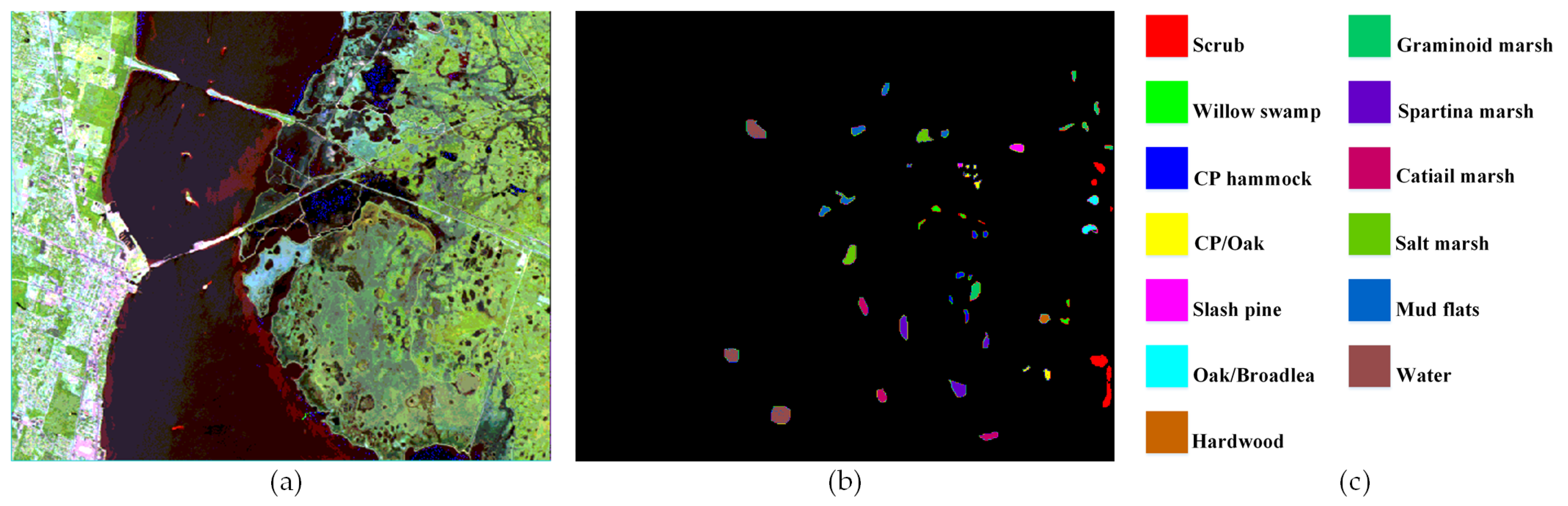
| 1 | Scrub | 761 |
| 2 | Willow | 243 |
| 3 | CP hammock | 256 |
| 4 | Slash pine | 252 |
| 5 | Oak/Broadleaf | 161 |
| 6 | Hardwood | 229 |
| 7 | Grass-pasture-mowed | 105 |
| 8 | Graminoid marsh | 431 |
| 9 | Spartina marsh | 520 |
| 10 | Cattail marsh | 404 |
| 11 | Salt marsh | 419 |
| 12 | Mud flats | 503 |
| 13 | Water | 927 |
| Total | 5211 |
| No. | Class Name | Numbers of Samples |
|---|---|---|
| 1 | Brocoli-green-weeds_1 | 391 |
| 2 | Com_senesced_green_weeds | 134 |
| 3 | Lettcue_romaine_4wk | 616 |
| 4 | Lettcue_romaine_5wk | 152 |
| 5 | Lettcue_romaine_6wk | 674 |
| 6 | Lettcue_romaine_7wk | 799 |
| Total | 5348 |
| Parameters Datasets | IN | KSC | SA |
|---|---|---|---|
| ratio of samples | 4:1:5 | 4:1:5 | 4:1:5 |
| spatial patch size | |||
| spectral patch size | |||
| batch size | 16 | 16 | 16 |
| epoch | 400 | 50 | 50 |
| optimizer | SGD | SGD | SGD |
| learning rate | 0.001 | 0.0005 | 0.001 |
| number of PCs | 30 | 30 | 30 |
| 0.02 | 0.02 | 0.02 | |
| number of MRCA | 8 | 8 | 8 |
| compressed ratio of CA | 1 | 4 | 1 |
| Data Set | Indexes Ratios | 0.5:1:8.5 | 1:1:8 | 2:1:7 | 3:1:6 | 4:1:5 |
|---|---|---|---|---|---|---|
| IN | OA | 64.22 | 94.54 | 99.10 | 98.97 | 99.74 |
| AA | 35.56 | 78.32 | 96.58 | 98.76 | 99.64 | |
| Kappa × 100 | 58.06 | 93.76 | 98.97 | 98.82 | 99.70 | |
| KSC | OA | 96.56 | 98.00 | 99.48 | 99.45 | 99.96 |
| AA | 95.28 | 97.27 | 99.40 | 99.33 | 99.94 | |
| Kappa × 100 | 96.12 | 97.78 | 99.42 | 99.39 | 99.96 | |
| SA | OA | 82.29 | 99.94 | 100 | 91.05 | 100 |
| AA | 68.61 | 99.91 | 100 | 81.43 | 100 | |
| Kappa × 100 | 77.25 | 99.92 | 100 | 88.70 | 100 |
| Class | SVM | MLR | RF | 1D-CNN | 2D-CNN | 3D-CNN | Hybrid | JSSAN | RSSAN | TSCCN | SMFFNet |
|---|---|---|---|---|---|---|---|---|---|---|---|
| 1 | 85.71 | 72.00 | 100.0 | 75.76 | 10.00 | 93.18 | 100.0 | 100.0 | 32.86 | 96.00 | 96.00 |
| 2 | 70.09 | 68.53 | 65.12 | 79.42 | 63.35 | 99.51 | 86.88 | 92.32 | 48.09 | 99.45 | 100.0 |
| 3 | 74.88 | 56.59 | 70.50 | 84.34 | 78.45 | 98.29 | 95.89 | 91.67 | 71.13 | 98.79 | 99.77 |
| 4 | 66.39 | 52.63 | 50.46 | 89.42 | 93.72 | 99.53 | 97.65 | 93.55 | 48.16 | 95.75 | 100.0 |
| 5 | 94.25 | 83.25 | 86.84 | 95.26 | 63.47 | 98.18 | 94.84 | 92.66 | 80.58 | 99.31 | 100.0 |
| 6 | 88.18 | 89.83 | 90.18 | 88.65 | 58.48 | 99.70 | 89.18 | 93.81 | 76.38 | 98.95 | 100.0 |
| 7 | 100.0 | 90.91 | 0 | 100.0 | 0 | 100.0 | 100.0 | 94.12 | 23.73 | 59.52 | 100.0 |
| 8 | 93.84 | 91.83 | 90.52 | 95.94 | 37.04 | 100.0 | 95.33 | 99.77 | 93.81 | 100.0 | 100.0 |
| 9 | 100.0 | 100.0 | 57.14 | 100.0 | 0 | 100.0 | 94.74 | 84.62 | 26.32 | 100.0 | 100.0 |
| 10 | 74.71 | 68.25 | 75.24 | 80.57 | 54.91 | 99.20 | 90.86 | 96.71 | 92.17 | 98.97 | 100.0 |
| 11 | 67.46 | 68.39 | 71.64 | 70.74 | 82.65 | 97.18 | 97.37 | 97.42 | 71.90 | 99.55 | 100.0 |
| 12 | 71.21 | 60.00 | 70.00 | 80.69 | 89.05 | 98.48 | 99.53 | 88.81 | 52.10 | 96.36 | 99.16 |
| 13 | 98.18 | 88.30 | 91.28 | 97.87 | 74.42 | 100.0 | 93.26 | 92.90 | 100.0 | 100.0 | 100 |
| 14 | 88.09 | 88.22 | 89.65 | 95.38 | 34.19 | 99.91 | 96.14 | 98.68 | 82.51 | 99.91 | 100 |
| 15 | 66.43 | 65.02 | 64.86 | 91.86 | 56.49 | 99.13 | 97.35 | 99.10 | 48.83 | 100.0 | 99.57 |
| 16 | 100.0 | 93.42 | 90.79 | 94.12 | 0 | 90.36 | 80.81 | 96.49 | 89.74 | 98.67 | 97.00 |
| OA | 76.41 | 73.22 | 70.02 | 82.32 | 58.32 | 98.66 | 93.89 | 95.26 | 66.94 | 98.98 | 99.74 |
| AA | 62.03 | 67.39 | 65.93 | 77.51 | 39.40 | 97.44 | 93.78 | 87.90 | 63.24 | 93.79 | 99.64 |
| Kappa ×100 | 72.83 | 69.24 | 72.50 | 79.55 | 51.76 | 98.47 | 93.03 | 94.60 | 62.14 | 98.84 | 99.70 |
| Class | SVM | MRL | RF | 1D-CNN | 2D-CNN | 3D-CNN | Hybrid | JSSAN | RSSAN | TSCNN | SMFF |
|---|---|---|---|---|---|---|---|---|---|---|---|
| 1 | 78.93 | 91.30 | 93.14 | 100.0 | 93.83 | 93.85 | 94.39 | 95.54 | 99.91 | 100.0 | 100.0 |
| 2 | 93.20 | 95.65 | 83.62 | 98.00 | 97.19 | 94.51 | 91.25 | 91.89 | 93.47 | 74.59 | 100.0 |
| 3 | 75.00 | 57.09 | 79.43 | 76.00 | 46.92 | 85.84 | 93.27 | 98.44 | 83.03 | 41.18 | 100.0 |
| 4 | 50.25 | 54.12 | 60.00 | 79.00 | 92.39 | 95.27 | 92.91 | 91.41 | 78.91 | 100.0 | 100.0 |
| 5 | 50.47 | 64.22 | 69.49 | 90.00 | 100.0 | 100.0 | 95.45 | 91.87 | 62.13 | 100.0 | 100.0 |
| 6 | 78.29 | 73.77 | 55.56 | 63.00 | 36.94 | 98.31 | 94.48 | 98.66 | 53.33 | 100.0 | 100.0 |
| 7 | 74.70 | 64.96 | 82.56 | 95.00 | 97.56 | 98.63 | 96.51 | 100.0 | 96.83 | 85.14 | 100.0 |
| 8 | 89.66 | 88.04 | 83.66 | 98.00 | 90.10 | 99.32 | 98.32 | 78.64 | 93.40 | 62.17 | 100.0 |
| 9 | 88.26 | 86.53 | 90.10 | 95.00 | 100.0 | 86.09 | 87.87 | 73.36 | 96.37 | 88.63 | 99.62 |
| 10 | 100.0 | 100.0 | 99.71 | 100.0 | 99.09 | 97.30 | 94.74 | 93.97 | 95.24 | 99.07 | 100.0 |
| 11 | 99.44 | 98.04 | 99.72 | 95.00 | 98.82 | 98.82 | 97.90 | 96.23 | 99.41 | 100.0 | 100.0 |
| 12 | 98.58 | 96.06 | 91.42 | 95.00 | 98.53 | 85.11 | 81.72 | 90.26 | 70.87 | 98.50 | 100.0 |
| 13 | 100.0 | 100.0 | 100.0 | 100.0 | 99.32 | 100.0 | 99.18 | 98.38 | 86.65 | 99.73 | 100.0 |
| OA | 87.89 | 87.72 | 88.53 | 92.54 | 83.10 | 94.18 | 93.48 | 90.69 | 86.59 | 89.89 | 99.96 |
| AA | 80.07 | 82.10 | 82.90 | 90.03 | 87.60 | 91.69 | 91.73 | 87.55 | 84.85 | 85.73 | 99.94 |
| Kappa ×100 | 86.48 | 86.33 | 87.23 | 92.54 | 83.58 | 93.51 | 92.73 | 89.61 | 85.11 | 88.75 | 99.96 |
| Class | SVM | MLR | RF | 1D-CNN | 2D-CNN | 3D-CNN | Hybrid | JSSAN | RSSAN | TSCNN | SMFF |
|---|---|---|---|---|---|---|---|---|---|---|---|
| 1 | 100.0 | 100.0 | 100.0 | 99.00 | 66.00 | 100.0 | 100.0 | 96.00 | 100.0 | 98.00 | 100.0 |
| 2 | 67.58 | 99.75 | 79.29 | 98.00 | 100.0 | 100.0 | 100.0 | 100.0 | 98.00 | 100.0 | 100.0 |
| 3 | 100.0 | 99.41 | 100.0 | 30.00 | 65.00 | 89.00 | 100.0 | 100.0 | 98.35 | 100.0 | 100.0 |
| 4 | 99.93 | 68.67 | 82.61 | 89.00 | 99.00 | 92.00 | 100.0 | 99.00 | 97.00 | 100.0 | 100.0 |
| 5 | 100.0 | 100.0 | 92.82 | 100.0 | 100.0 | 100.0 | 100.0 | 98.00 | 95.85 | 100.0 | 100.0 |
| 6 | 100.0 | 99.86 | 96.88 | 99.00 | 100.0 | 100.0 | 99.00 | 97.00 | 90.00 | 99.00 | 100.0 |
| OA | 87.99 | 87.00 | 86.64 | 72.08 | 89.50 | 96.05 | 99.90 | 98.69 | 96.32 | 99.69 | 100.0 |
| AA | 81.71 | 82.85 | 80.31 | 83.38 | 88.36 | 95.86 | 99.86 | 98.26 | 96.39 | 99.70 | 100.0 |
| Kappa ×100 | 84.68 | 83.32 | 82.91 | 66.95 | 87.30 | 95.05 | 99.87 | 98.36 | 95.40 | 99.61 | 100.0 |
| Data Set | Indexes Schemes | ReLU | Sigmoid | ReLU+L2 | Sigmoid+L2 |
|---|---|---|---|---|---|
| IN | OA | 99.37 | 96.85 | 98.10 | 99.74 |
| AA | 98.67 | 78.99 | 96.25 | 99.64 | |
| Kappa × 100 | 99.28 | 96.85 | 97.83 | 99.70 | |
| KSC | OA | 96.30 | 96.34 | 99.92 | 99.96 |
| AA | 91.76 | 92.37 | 99.87 | 99.94 | |
| Kappa × 100 | 95.88 | 95.92 | 99.91 | 99.96 | |
| SA | OA | 100.0 | 100.0 | 100.0 | 100.0 |
| AA | 100.0 | 100.0 | 100.0 | 100.0 | |
| Kappa × 100 | 100.0 | 100.0 | 100.0 | 100.0 |
| Data Set | Indexes Schemes | NO-Net | CAM-Net | SAM-Net | CAM+SAM-Net |
|---|---|---|---|---|---|
| IN | OA | 92.46 | 98.49 | 99.25 | 99.74 |
| AA | 74.31 | 93.34 | 97.80 | 99.64 | |
| Kappa × 100 | 91.38 | 98.28 | 99.15 | 99.70 | |
| KSC | OA | 89.97 | 90.74 | 93.02 | 99.96 |
| AA | 79.19 | 78.47 | 83.09 | 99.94 | |
| Kappa × 100 | 88.82 | 89.69 | 92.23 | 99.96 | |
| SA | OA | 79.90 | 100.0 | 98.82 | 100.0 |
| AA | 75.64 | 100.0 | 99.28 | 100.0 | |
| Kappa × 100 | 74.39 | 100.0 | 98.52 | 100.0 |
Publisher’s Note: MDPI stays neutral with regard to jurisdictional claims in published maps and institutional affiliations. |
© 2021 by the authors. Licensee MDPI, Basel, Switzerland. This article is an open access article distributed under the terms and conditions of the Creative Commons Attribution (CC BY) license (https://creativecommons.org/licenses/by/4.0/).
Share and Cite
Liu, D.; Han, G.; Liu, P.; Yang, H.; Sun, X.; Li, Q.; Wu, J. A Novel 2D-3D CNN with Spectral-Spatial Multi-Scale Feature Fusion for Hyperspectral Image Classification. Remote Sens. 2021, 13, 4621. https://doi.org/10.3390/rs13224621
Liu D, Han G, Liu P, Yang H, Sun X, Li Q, Wu J. A Novel 2D-3D CNN with Spectral-Spatial Multi-Scale Feature Fusion for Hyperspectral Image Classification. Remote Sensing. 2021; 13(22):4621. https://doi.org/10.3390/rs13224621
Chicago/Turabian StyleLiu, Dongxu, Guangliang Han, Peixun Liu, Hang Yang, Xinglong Sun, Qingqing Li, and Jiajia Wu. 2021. "A Novel 2D-3D CNN with Spectral-Spatial Multi-Scale Feature Fusion for Hyperspectral Image Classification" Remote Sensing 13, no. 22: 4621. https://doi.org/10.3390/rs13224621
APA StyleLiu, D., Han, G., Liu, P., Yang, H., Sun, X., Li, Q., & Wu, J. (2021). A Novel 2D-3D CNN with Spectral-Spatial Multi-Scale Feature Fusion for Hyperspectral Image Classification. Remote Sensing, 13(22), 4621. https://doi.org/10.3390/rs13224621