Abstract
Rangelands are composed of patchy, highly dynamic herbaceous plant communities that are difficult to quantify across broad spatial extents at resolutions relevant to their characteristic spatial scales. Furthermore, differentiation of these plant communities using remotely sensed observations is complicated by their similar spectral absorption profiles. To better quantify the impacts of land management and weather variability on rangeland vegetation change, we analyzed high resolution hyperspectral data produced by the National Ecological Observatory Network (NEON) at a 6500-ha experimental station (Central Plains Experimental Range) to map vegetation composition and change over a 5-year timescale. The spatial resolution (1 m) of the data was able to resolve the plant community type at a suitable scale and the information-rich spectral resolution (426 bands) was able to differentiate closely related plant community classes. The resulting plant community class map showed strong accuracy results from both formal quantitative measurements (F1 75% and Kappa 0.83) and informal qualitative assessments. Over a 5-year period, we found that plant community composition was impacted more strongly by weather than by the rangeland management regime. Our work displays the potential to map plant community classes across extensive areas of herbaceous vegetation and use resultant maps to inform rangeland ecology and management. Critical to the success of the research was the development of computational methods that allowed us to implement efficient and flexible analyses on the large and complex data.
1. Introduction
Herbaceous plant community composition is a strong driver of ecosystem function [1], herbivore foraging dynamics [2,3], and wildlife habitat quality [4,5] in semi-arid rangeland systems. In many regions, the composition of herbaceous species is highly dynamic over space and time due to the complex influences of multiple, interactive drivers including soil type, topography, weather and climate, herbivory, fire, small mammal disturbance, and more [6,7,8,9,10,11]. Characterizing plant communities and plant community change across broad rangeland landscapes at process-relevant scales is critical to understand the impacts of management, disturbance, and the changing climate.
Despite the importance of plant species composition in grasslands, data at management-relevant scales are hard to obtain. Mapping efforts tend to lump herbaceous vegetation into a single class (e.g., NLCD; [12] or, at best, differentiate only between annual and perennial grasses (RAP; [13]), primarily because measuring this critical ecosystem property is time-consuming and difficult to automate. Individual herbaceous plants in these systems are often quite small and dozens of species can be intermingled at very fine (sub-meter) scales (e.g., [14]). Field-based data collection typically takes place at spatial resolutions ranging from sub-meter to ~1 ha. To scale-up from these fine-scaled but area-limited field measurements to information that would be relevant at larger scales (e.g., livestock paddocks or wildlife home ranges), researchers have commonly extended plant community findings via the stratification of large areas based on more easily measured properties such as topography, known histories of disturbance, or soil types [15].
These stratification approaches have power, particularly when multiple drivers are considered. For example, ecological site descriptions derived from national soil maps and their associated state-and-transition models provide detailed information about the potential plant community types that may be present in a given location [16] and typically describe the interactive effects of soil type, climate or weather, and management drivers. Similarly, catena-based approaches provide information about how topography can modify both plant community composition and aspects of ecosystem function [9,17,18]. However, few of these approaches can directly map and monitor complex spatial patterns of plant community composition on the ground or detect how the composition changes over time across broad scales.
High spatial resolution, remotely sensed data provide a potential solution to the problem of mapping and monitoring plant community composition. In recent years, efforts to map the cover of basic plant functional groups have advanced dramatically and are now being applied at regional-to-continental scales [13,19]. Such approaches are unable to differentiate among grassland plant community types or associations due to the broadband wavelengths and coarse resolution inherent to the imagery available for large spatial regions (e.g., Landsat, Sentinel, and MODIS). This is especially problematic in grasslands where many species are intermingled at sub-meter spatial scales.
Hyperspectral imagery collected at high spatial resolution shows promise for further resolving fine-scale heterogeneity within grasslands. Hyperspectral imagery has been used across a wide range of grassland ecosystems to map plant traits [20,21,22], plant communities [23,24], and individual species. While mapping individual species may be considered the “holy grail” for classification and could be used to derive maps of plant communities and functional groups, the high diversity of species present at very fine spatial scales makes it impractical to map all, or even most, species across large areas. As a result, species mapping has so far either focused on detecting one or two wide-spread invasive grasses (e.g., [25,26]) or has been completed for very small areas (e.g., [14]). Developing methods that utilize fine-scale hyperspectral imagery to map grassland plant communities is critical to addressing long-standing and emerging grassland management issues, such as assessing the impacts of climate change, conserving the integrity of wildlife habitats, and optimizing grazing management practices.
Here, we used publicly available, fine-scale (1 m pixel) hyperspectral data obtained by the National Ecological Observatory Network (NEON) Airborne Observatory Platform (AOP) to map herbaceous plant community types and their spatial and temporal dynamics in a shortgrass steppe ecosystem. This work was conducted at the Central Plains Experimental Range (CPER), a site within the Long-Term Agroecosystem Research (LTAR) network. The site is dominated by perennial herbaceous vegetation, but within this “grassland context”, plant community composition is variable in space and time, with consequences for livestock production, wildlife conservation, and ecosystem function. The goals of this project were to:
- Develop advanced plant community composition classification methods that could be used to map plant composition at our site and at other NEON sites or in areas with similar hyperspectral data;
- Determine the utility of plant community mapping for detecting the effects of soil type, weather, management, and ecological disturbances (e.g., burrowing mammals) on plant community composition and compositional change over time.
2. Materials and Methods
2.1. Study Area
This research was conducted at the USDA ARS Central Plains Experimental Range (CPER), a Long-Term Agroecosystem Research as well as a NEON core terrestrial site (Domain 10), located in northeastern Colorado (40°49′N, 107°46′W; Figure 1). The study area is dominated by shortgrass steppe vegetation and is characterized by a mix of perennial warm-season (C4) and cool-season (C3) graminoids. Blue grama (Bouteloua gracilis) is the dominant warm season grass species, with buffalograss (B. dactyloides) as the subdominant species. Dominant perennial cool-season graminoids include needle-and-thread (Hesperostipa comata), needle-leaf sedge (Carex duriuscula), and western wheatgrass (Pascopyrum smithii). The dominant forb and subshrub are scarlet globemallow (Sphaeralcea coccinea), and fringed sagewort (Artemisia frigida Willd.), respectively. Plains pricklypear cactus (Opuntia polyacantha Haw.) is also common. Annual grasses consist almost entirely of six-weeks fescue (Vulpia octoflora, plant nomenclature derived from https://plants.usda.gov, accessed on 4 November 2021). The mean annual precipitation is 34 cm, and the mean annual temperature is 8.4 °C, ranging from −2.6 °C in December to 21.3 °C in July.
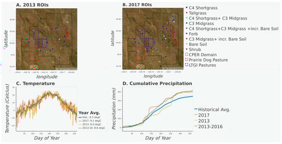
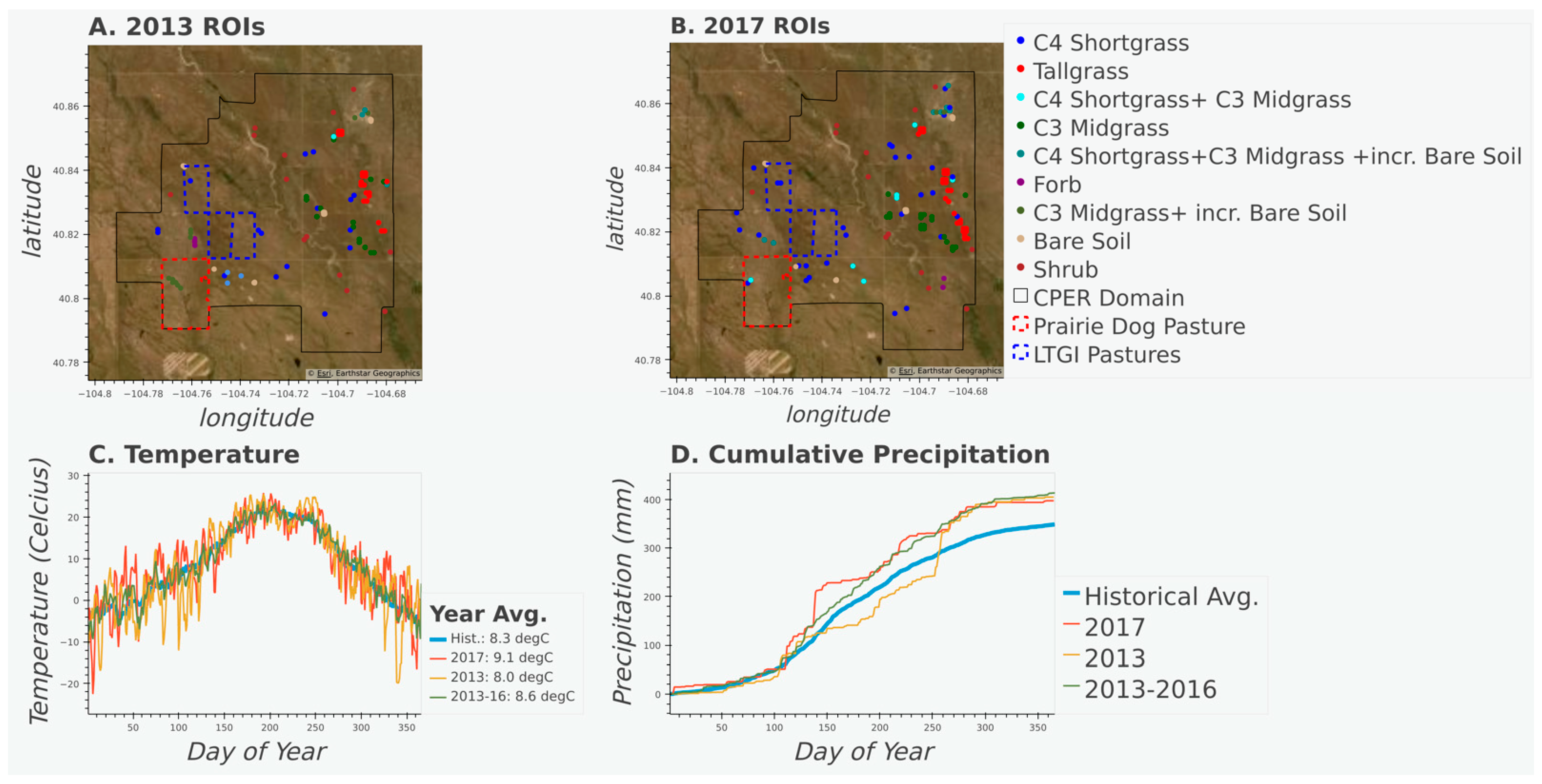
Figure 1.
Maps displaying the aerial imagery of the study area, vegetation transect locations, pasture of interest (see Section 3.2), and CPER domain for 2013 (A) and 2017 (B). Time series of temperature (C) and cumulative precipitation (D) for 2013, 2017 and averaged values from 2013 to 2016, and the historical (1981–2020) record. Temperature and precipitation data from PRISM ANSI81.
2.2. In situ Vegetation Data
We measured plant foliar cover by species at 112 plots distributed across 25 different 130-ha pastures at CPER in mid-June of both 2013 and 2017 as part of a collaborative adaptive grazing management experiment [27]). Pastures were stratified by ecological site and topography, and monitoring plots were established within the strata for each pasture. We established 4 pairs of plots in each of the 19 pastures containing 1 or 2 strata (loamy and/or sandy plains ecological sites), and 6 plots in each of 6 pastures that contained 3 strata (loamy plains, sandy plains, and salt flats). Each plot contained a systematic grid of 4, 25-meter transects oriented north-south and spaced 106 m apart (n = 448 total transects). Along each transect, technicians used the line-point intercept method [28] to quantify the species composition of the plant community by passing a laser vertically through the canopy at 50 locations per transect, spaced at 0.5 m intervals. At each location, they recorded the first species contacted by the laser, or if no vegetation was contacted, they recorded whether the laser contacted bare soil or litter. Intercepts contacting current-year vegetation growth were recorded by species, but intercepts contacting standing dead vegetation carried over from the prior year (identified by a dull, grey color) were simply recorded as “standing dead” without regard to the species. In 2017, we added 4 new plots in one additional pasture (16 transects) for a total of 464 transects sampled.
These data were used to calculate the percent cover of 12 plant functional groups (Table 1). We included contacts with dung and lichen in the litter category. In addition, we counted the number of tillers of Pascopyrum smithii and the number of individuals of Hesperostipa comata in 0.25 m2 quadrats placed at 3 m intervals along each transect (n = 8 quadrats per transect) to obtain a second measure of the abundance of these two important but less abundant forage species. For these two species, canopy cover estimates can be imprecise when the plants occur at low relative abundance, in part because they have more vertically oriented leaves compared to the other grass and forb species. Our estimates of plant abundance for these species based on counts in 0.25 m2 quadrats were more precise than our canopy interception-based estimates when these species were rare, because of the larger area sampled using the density method compared to canopy interception. We adjusted the cover estimates for these two species using the density measurements as follows. First, we regressed plant density (tillers or individuals per m2 based on the 0.25 m2 quadrats) against percent cover estimated via canopy interception at the scale of each transect. We used this regression to estimate the percent cover of each species predicted based on the measurement of plant density. We then calculated the estimate of percent cover for these two species in each transect as the sum of the estimate based on canopy interception and the estimate based on plant density, divided by two.

Table 1.
The twelve plant functional groups used in a cluster analysis to identify distinct plant communities to be mapped using hyperspectral imagery at the Central Plains Experimental Range in northeast Colorado.
Due to the fine-scale interspersion of plant functional groups within a transect, we conducted a cluster analysis of the transect by a functional group matrix based on measurements from both 2013 and 2017. We used a hierarchical, agglomerative, numerical cluster analysis based on Euclidean distances and Ward’s method for the determination of group linkages (implemented in PC-ORD v6.0) and conducted 5 different analyses that clustered transects into 12, 11, 10, 9, and 8 groups, respectively. After examining group membership and associated dendrograms, we used the 8-group cluster analysis to identify distinct plant community classes. Four classes were dominated by C4 shortgrasses but contained varying levels of subdominant species and bare soil (see y-axis in Figure 2). The remaining four classes identified communities consisting of (1) C3 midgrasses (Hesperostipa comata, Pascopyrum smithii, and Elymus elymoides) dominant, (2) C3 midgrasses dominant, with high exposure of bare soil, (3) C4 saltgrasses with C3 midgrasses (hereafter Tallgrass) dominant, and (4) forbs dominant (Figure 2).
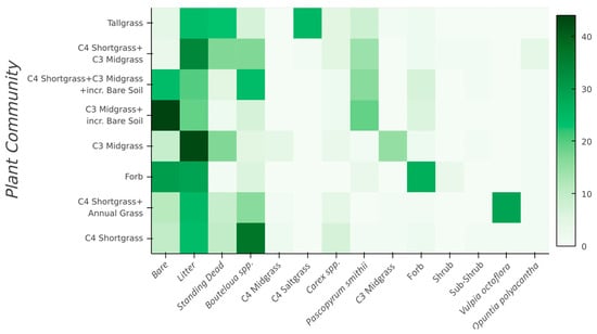
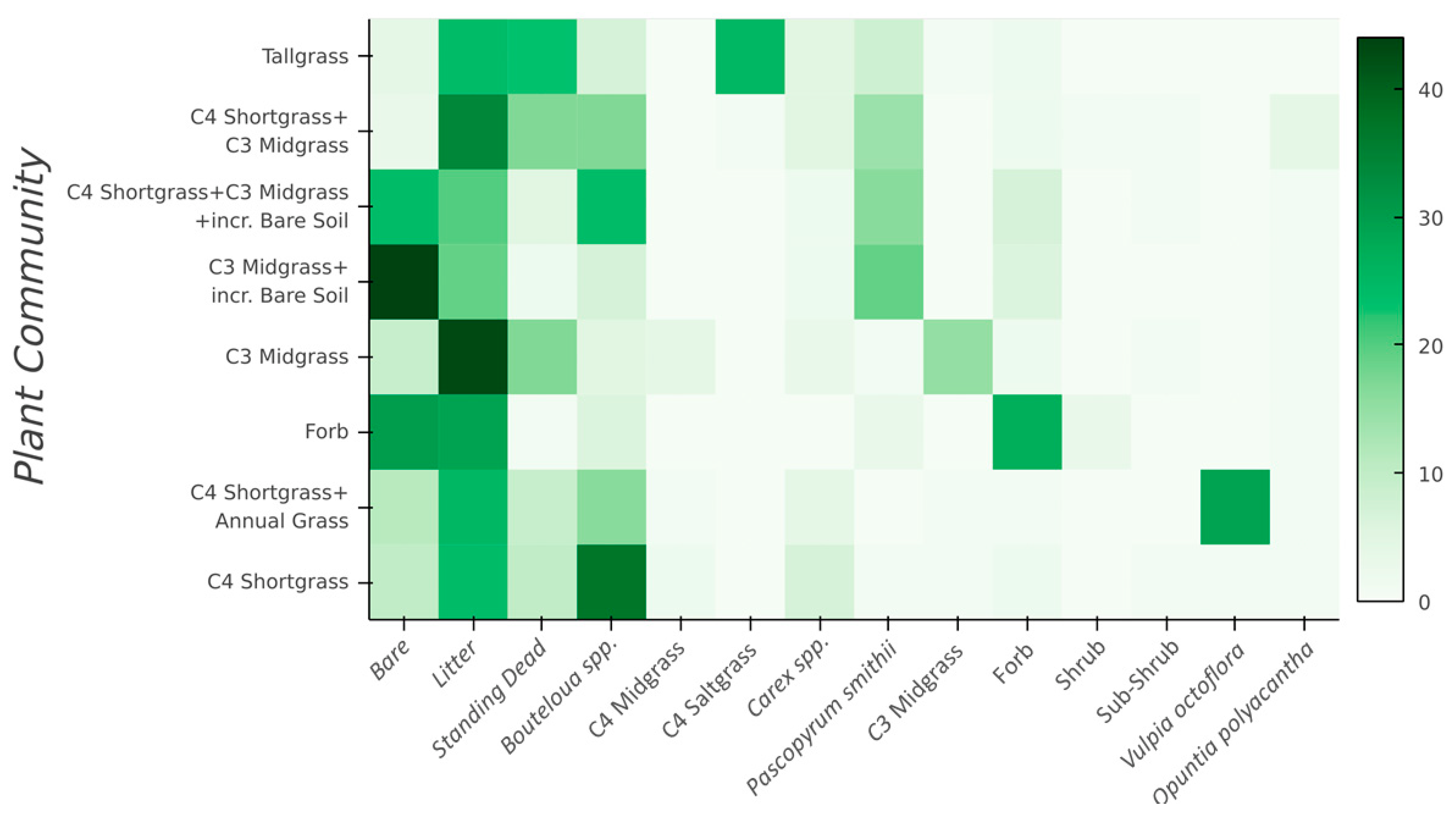
Figure 2.
Average plant community class (Y-axis) composition derived from the 175 vegetation transects throughout CPER. The vegetation components on the X-axis are directly related to Table 1, except Bouteloua spp. = C4 Shortgrasses, and C3 Midgrass = C3 Needle and thread (Hesperostipa comata) + C3 Squirreltail (Elymus elymoides).
To define plant community class endmembers to use as training data for the hyperspectral imagery mapping, we then selected a subset of transects within each of these 8 groups, where the selected subset was most representative of the defined community. For example, of the 175 transects classified in the “C4 shortgrass” cluster, cover of C4 shortgrasses, litter, and bare soil varied from 32–73%, 6–32%, to 0–27%, respectively. To represent the endmember for this plant community, we selected a subset of 16 transects where C4 shortgrass cover was >50% (range 51–61%), while litter cover was still in the range of 8–20% and bare soil in the range of 6–20% (Figure 2). This approach provided plant community classes with high cover of the characteristic dominant and/or subdominant species, while removing from the calibration those transects with high compositional variability. This process identified 175 transects representing 8 plant community classes that correspond to common, uniquely identifiable, and ecologically important plant communities at CPER (Figure 2). However, the transects were not evenly distributed across the plant community classes, ranging from 4 to 48 transects per class.
To link the transects and airborne hyperspectral data, a 2-m radius around each transect defined a region of interest (ROI), which was used to query the hyperspectral data. This approach provided ~120-pixel observations per transect, resulting in a data cloud large enough to permit machine learning classification models described below (Section 2.3).
2.3. Hyperspectral Data
Hyperspectral reflectance data (NEON product DP1.30006.001) were acquired by the NEON AOP at the CPER domain on 25 June 2013, and 24 May 2017 [29]. For each year, 26 North–South (N–S) acquisition flights covered the entire CPER domain as well as a single overlapping East–West flight. We found strong East–West illumination trends within the N–S flight data, which we attributed to anisotropic reflectance. Therefore, the NEON AOP team applied additional BRDF corrections using the HyTools package [30]. Furthermore, the reflectance data were subset to specific spectral bands to exclude regions known to have H20 or CO2 absorption issues and spectral wavelengths that exhibited high variation or suspect spatial patterns.
To mosaic the overlapping flights into a single dataset, we selected pixels with a zenith angle nearest to NADIR. To improve the overall illumination consistency between flights, each N–S flight’s brightness was scaled to match the E–W flight observation based on regions of overlapping pixels with zenith angles of less than 6 degrees.
The transects used for our cluster analysis were intentionally located in the most dominant plant community types within each pasture, and therefore we needed additional approaches to map certain important but rare vegetation classes. To map bare ground and standing dead vegetation, we calculated a set of narrow and broad band vegetation indices from the hyperspectral reflectance data. These indices were added into the classification process as covariates. Bare-ground and standing dead classes were developed from the relationship between the cellulose absorption index (CAI) and the Normalized Differenced Vegetation Index (NDVI) [31,32]. Regions exhibiting spectral characteristics indicative of bare-ground and standing dead vegetation (Figure 3) were subsampled across the CPER domain at spatial strides of 6 and 22 meters for standing dead as well as 2 and 3 meters for bare-ground (2013 and 2017, respectively) to develop the training and validation data.
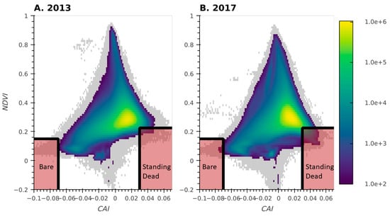
Figure 3.
Two-dimensional histogram of CAI-NDVI for 2013 (A) and 2017 (B). Shaded regions indicate the space used to extract Bare Ground and Standing Dead data for the training and validation of the classification model. Grey regions represent regions with fewer than 100 pixels per bin.
Additionally, high resolution RGB images collected during the NEON AOP flight in 2013 were used to develop ROIs for two additional vegetation communities: shrubs and bare soil. Large shrubs, visible in the imagery, were manually delineated across the entire CPER domain, while large patches dominated by bare soil were delineated within several pastures, generally near stock tanks or pasture corners (highly trafficked areas). We chose to include the bare-soil class in addition to the bare-ground class because the bare-ground spectral region (defined from Figure 3) mapped primarily to gravel roads and sandy stream beds, whereas the bare-soil class represented patches of the landscape with very low vegetation cover and a high proportional cover of exposed soil.
2.4. Vegetation Classification
Prior to classifying the hyperspectral data into plant community classes, we split the data into training (~75%) and testing (e.g., independent validation, ~25%) groups randomly (Figure 4). To incorporate the effect of spatial autocorrelation and variability between flight acquisitions on the accuracy assessment, we split the training and testing data (excluding the standing dead and bare ground classes, which were thoroughly distributed across the domain) by ROI (e.g., transect), rather than the pixel level. Splitting by ROI, rather than by pixel, insured that the “hold-out” data were completely independent from the model training data, resulting in a more conservative approach to quantify the overall accuracy of the model.

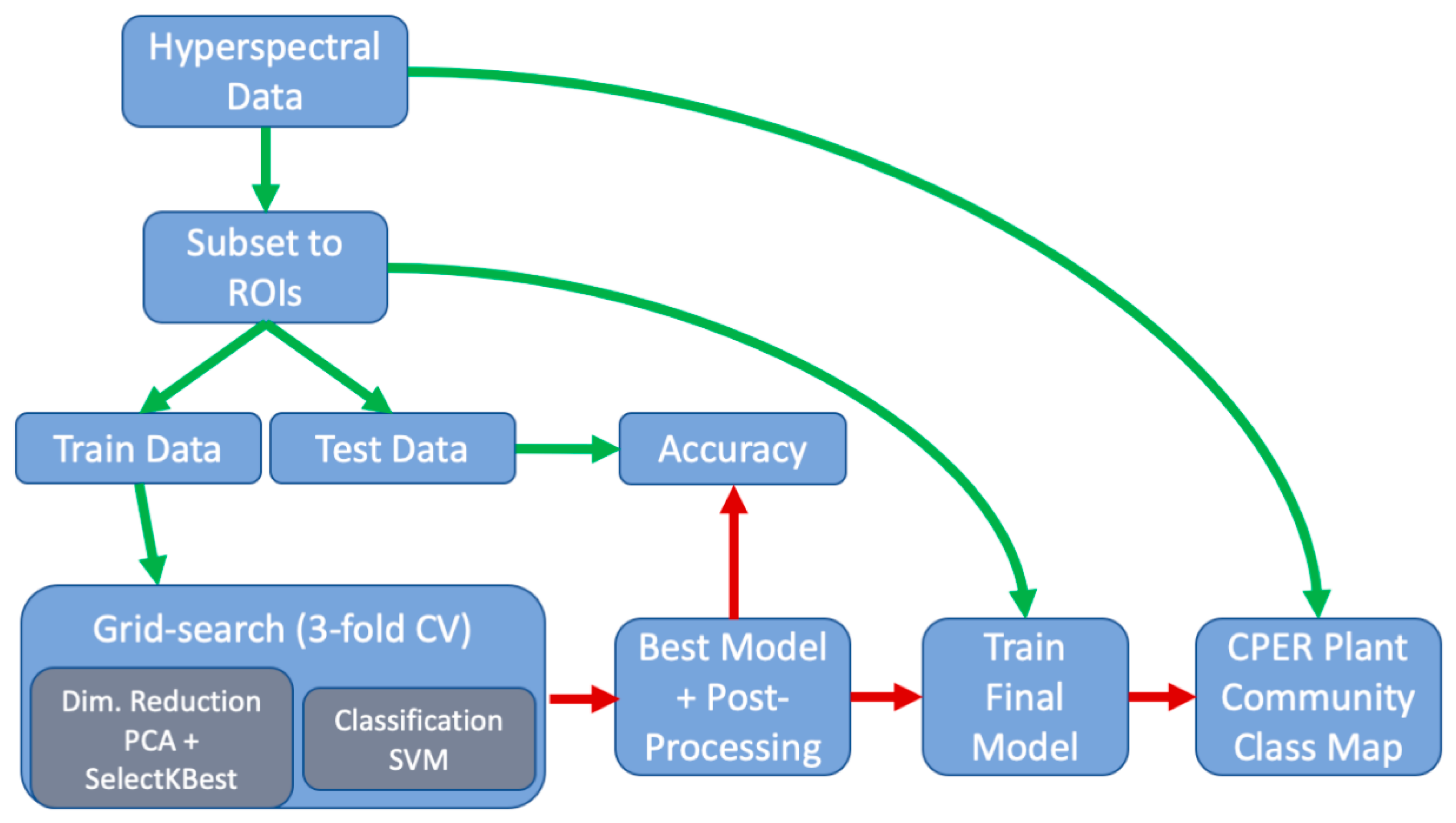
Figure 4.
Schematic showing the workflow/pipeline used in the classification process. Green arrows indicate the flow of data and red arrows indicate the flow of the machine learning model.
The classification algorithm involved two steps: (1) dimensional reduction using a combination of principal component analysis (PCA) and SelectKBest and (2) classification using a Support Vector Machine (SVM with a gaussian radial basis function kernel) algorithm using the Scikit-learn package [33]. An exhaustive grid-search approach was used to select the optimum number of dimensions (concurrently between PCA and SelectKbest), as well as the hyperparameters associated with the SVM model (C and gamma[γ]) (Table 2), using a 3-fold cross validation strategy maximizing the F1 accuracy statistic (weighted harmonic mean of precision and recall).
Table 2.
Grid-search parameter space used to optimize the model. The model parameters associated with the best-fit model are in bold. (see Section 3).
Once we identified the best-fit hyperparameters from the grid-search routine, we retrained the algorithm using these parameters and the entire training dataset. Using the results of this model, we calculated probabilities and defined a probability threshold for each class that maximized accuracy while minimizing the number of unclassified pixels. For each class, the probability threshold was increased until the true positivity rate dropped below 90% or the probability threshold reached 75%.
With the optimized hyperparameters, the accuracy of the model was assessed with the remaining testing data. The model was trained with the entire training dataset (~75%) and then predicted using the testing data (~25%). The probabilities were calculated for each pixel, and the thresholds previously calculated for each class were applied to the results. Finally, the overall accuracy of the model was quantified using F1 statistics (macro and micro), the Cohen Kappa score, and recall, precision, and confusion matrices.
2.5. Case Studies: Change Detection and Disturbance Impacts
In systems where C3 and C4 graminoids are mixed, shifts in relative abundance between these two functional types can have large impacts on ecosystem function [1] and the provision of wildlife habitats [5]. To assess the ability of our approach to capture temporal shifts between C3-dominated and C4-dominated plant community classes, we quantified shifts between the plant communities dominated by C4 species (C4 shortgrass) and plant communities that had significant C3 species (C3 Midgrass, C3 Midgrass + incr. Bare Soil, C3 Midgrass + C4 Shortgrass + incr. Bare Soil, and C3 Midgrass + C4 Shortgrass) from 2013 to 2017. On a 10 × 10-meter grid, we calculated the percent area that transitioned between the C4-dominated and C3-dominated classes between 2013 and 2017. We then differenced the C3-dominated and C4-dominated datasets between 2013 and 2017 to produce relative change maps across the CPER domain.
As additional case studies to assess the potential utility of our classification approach, we visually determined how well our classified map was able to detect and spatially quantify the impacts of two well defined and thoroughly studied disturbances at CPER: an 80-year grazing intensity experiment [34,35] and colonies of black-tailed prairie dogs (Cynomys ludovicianus; [36]).
The boundaries of active prairie dog colonies at CPER are mapped annually (see Augustine et al. 2014). To demonstrate the ability of our approach to detect fine-scale compositional impacts of prairie dog activity, we visually determined whether a commonly used soils dataset, SSURGO, or our plant community composition map was better able to visually resolve the impacts of the colonies on plant communities.
Starting in 1939, the Long-Term Grazing Experiment (LTGI; [34,37] has consistently applied three distinct cattle grazing intensities: light (20% utilization of peak growing season biomass), moderate (40% utilization), and heavy (60% utilization), from mid-May to October with season-long grazing on three adjoining ~130-hectare pastures (Figure 1). The differential grazing pressure resulted in a significantly elevated level of C3 plant communities in the lightly grazed pasture as compared to the moderately and heavily grazed pastures [35]. For the three pastures in the grazing experiment, we compared histograms of the mapped plant community classes between a pasture grazed heavily for 80 years and a pasture grazed lightly for 80 years to quantify the compositional impacts of grazing at the whole-pasture scale.
2.6. Computational Environment
The high dimensionality and volume associated with the NEON hyperspectral data posed considerable computational challenges. For instance, the total number of pixels from the 2013 NEON flight observations was greater than 211 million, resulting in over 90 billion observations (426 bands per pixel). To overcome these hurdles, we developed our analysis on the USDA ARS High Performance Computer (HPC) system (Ceres) using an open-source software stack in Python to distribute computations across multiple nodes. The data were processed, and machine learning algorithms were implemented in a distributed computing environment. To allow for reproducibility and extensibility, the computational environment was containerized using Docker [38] and is archived on DockerHub. The analysis was conducted in the Jupyter interface [39] with a wide breadth of geospatial and computational python tools [40]. The primary Python packages used in the analyses were Dask (distributed computing; [41,42]), Xarray (multi-dimensional arrays; [43]), SciKit-Learn (machine learning; [33]) and the Holoviews stack (visualizations; [44,45,46]).
3. Results
3.1. Accuracy and Plant Community Change
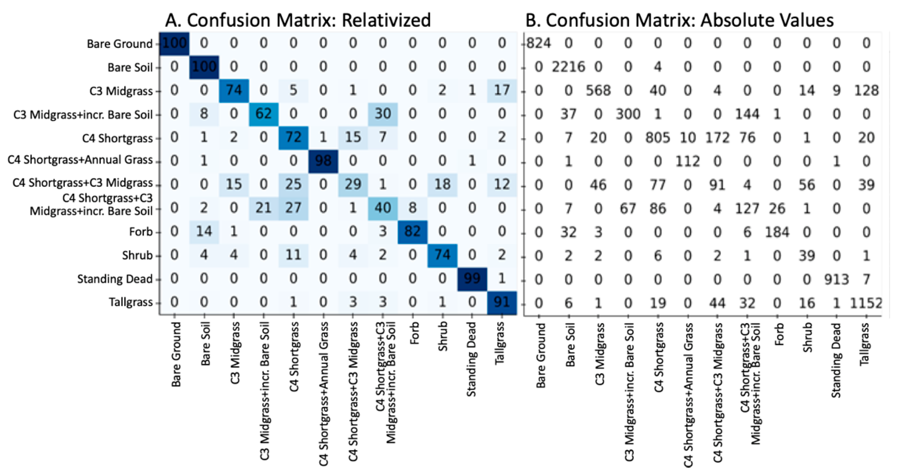
The overall accuracy assessment of the plant community classification produced a Cohen Kappa score of 0.826 and F1 scores of 85.5% (micro) and 74.9% (macro). Confusion matrices and tabulated accuracy metrics (Figure 5 and Table 3) show the overall and the individual plant community class accuracy of the classification while the mapped results of the classification are shown in Figure 6. Typically, plant community classes with more distinct species compositions were more accurately mapped than plant communities with more overlap within their species distributions. Despite our efforts to minimize the effect of the imbalanced training data (e.g., using the F1-Macro statistic to score the SVM model), there is a general trend towards higher accuracy within plant communities with larger training observations, typical of most machine learning algorithms. Overall, however, these results show that the pre-processing and machine learning approaches were able to accurately resolve the spectrally similar plant communities across CPER using hyperspectral data.
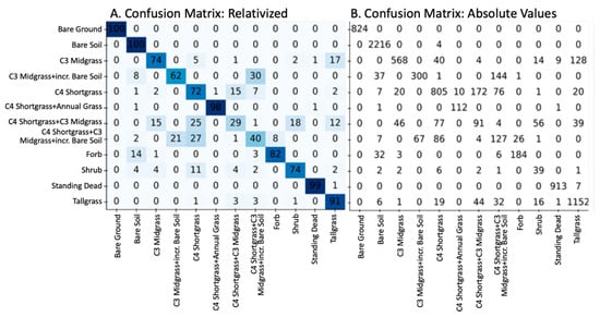
Figure 5.
Confusion matrices showing the relative (A) and absolute (B) results of the SVM model using the validation (hold-out) data. Rows are the actual values, and the columns are the predicted values.
Table 3.
A detailed accuracy assessment for each plant community class showing the precision, recall, and F1-Score for each class.
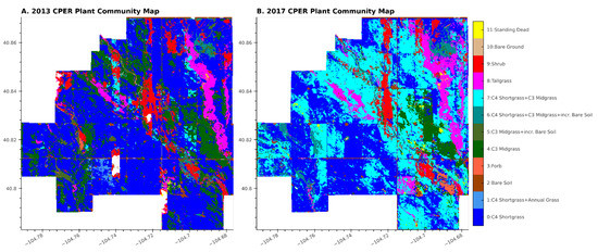
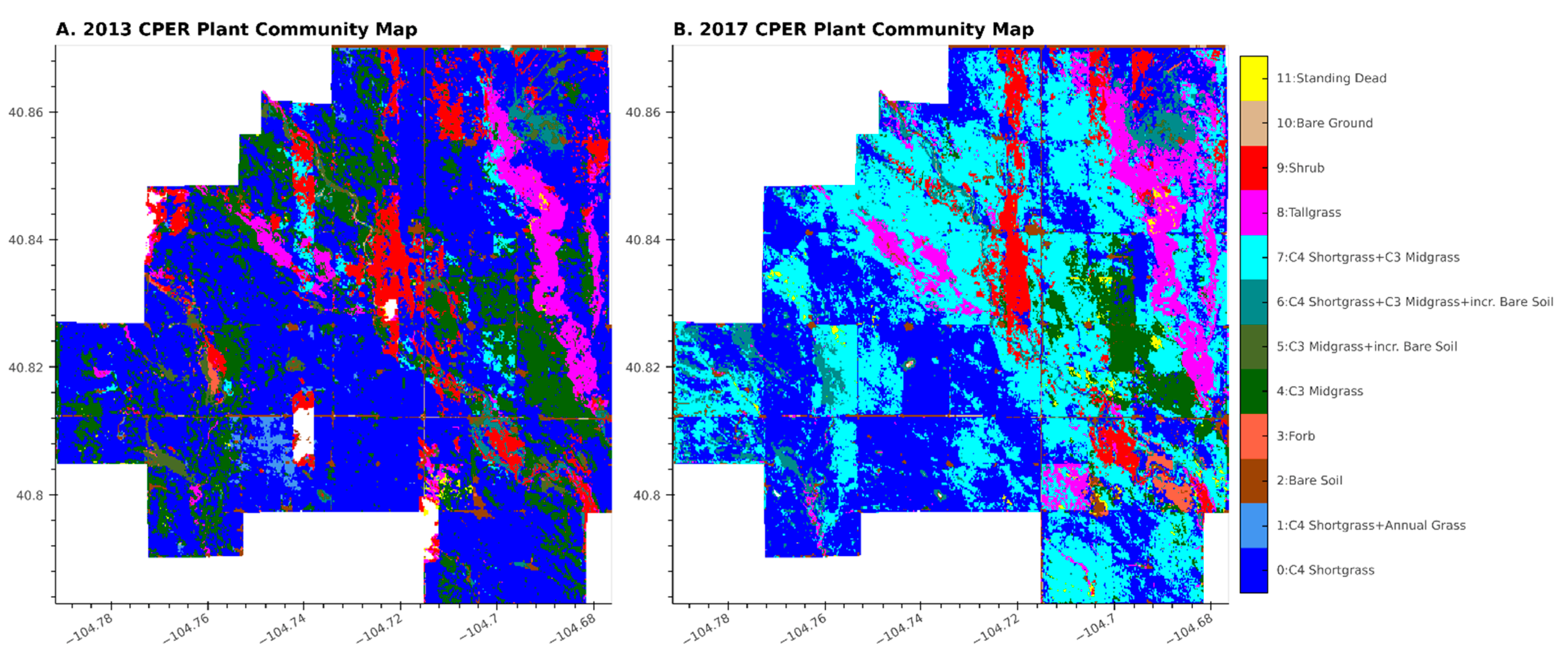
Figure 6.
Mapped results of the classification pipeline showing the plant community classes for 2013 (A) and 2017 (B).
To characterize plant community shifts between 2013 and 2017, we visualized the pixel-level changes using a Sankey Diagram (Figure 7). Within the plant community classes, the most prevalent transition was from C4 Shortgrass-dominated areas in 2013 to a C4 Shortgrass + C3 Midgrass community in 2017, which accounted for nearly 20% of the pixels. Augustine et al. [27] reported similar results based on ground-based observations of species compositional change between 2013 and 2017. The next-most prevalent shift was from the C3 Midgrass community to the C4 Shortgrass + C3 Midgrass community (3.4% of pixels).
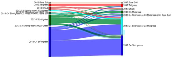
Figure 7.
Sankey plot detailing the change in plant communities from 2013 to 2017. For clarity, plant community classes that accounted for less the 0.5% of the change were excluded from this plot.
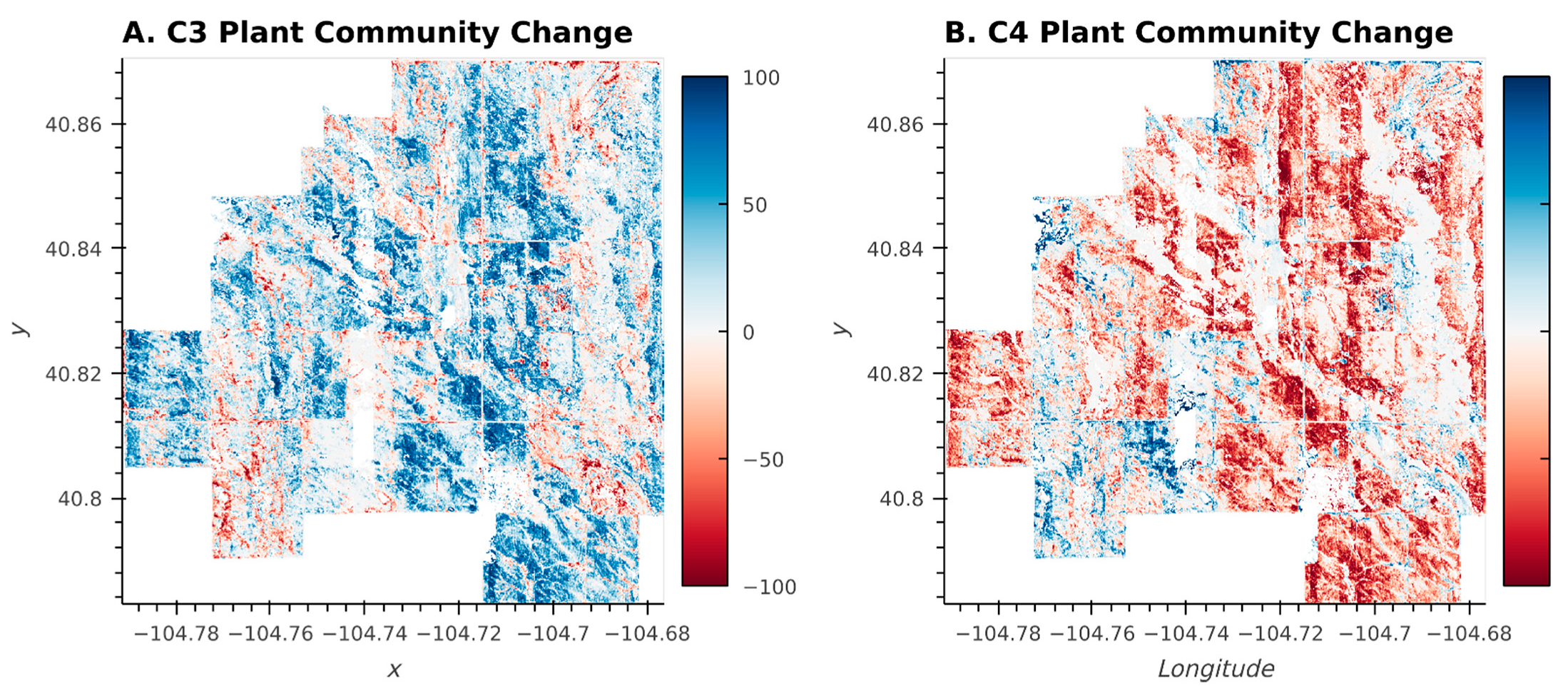
The plant community changes illustrated in the Sankey Diagram (Figure 7) were pervasive across many different pastures at the CPER, despite different management regimes being applied in different pastures (Figure 8; [27]). The magnitude and spatial extensiveness of the shift suggest that broad-scale drivers (such as shifting weather or climate patterns, Figure 1) were a stronger driver of plant community shifts between 2013 and 2017 than pasture-scale drivers (such as management practices) during this timeframe.

Figure 8.
Percent change in plant community classes dominated by C3 (A) and C4 (B) species between 2013 and 2017. Blue indicates an increase between 2013 and 2017 while red indicates a decrease.
3.2. Characterizing Disturbances
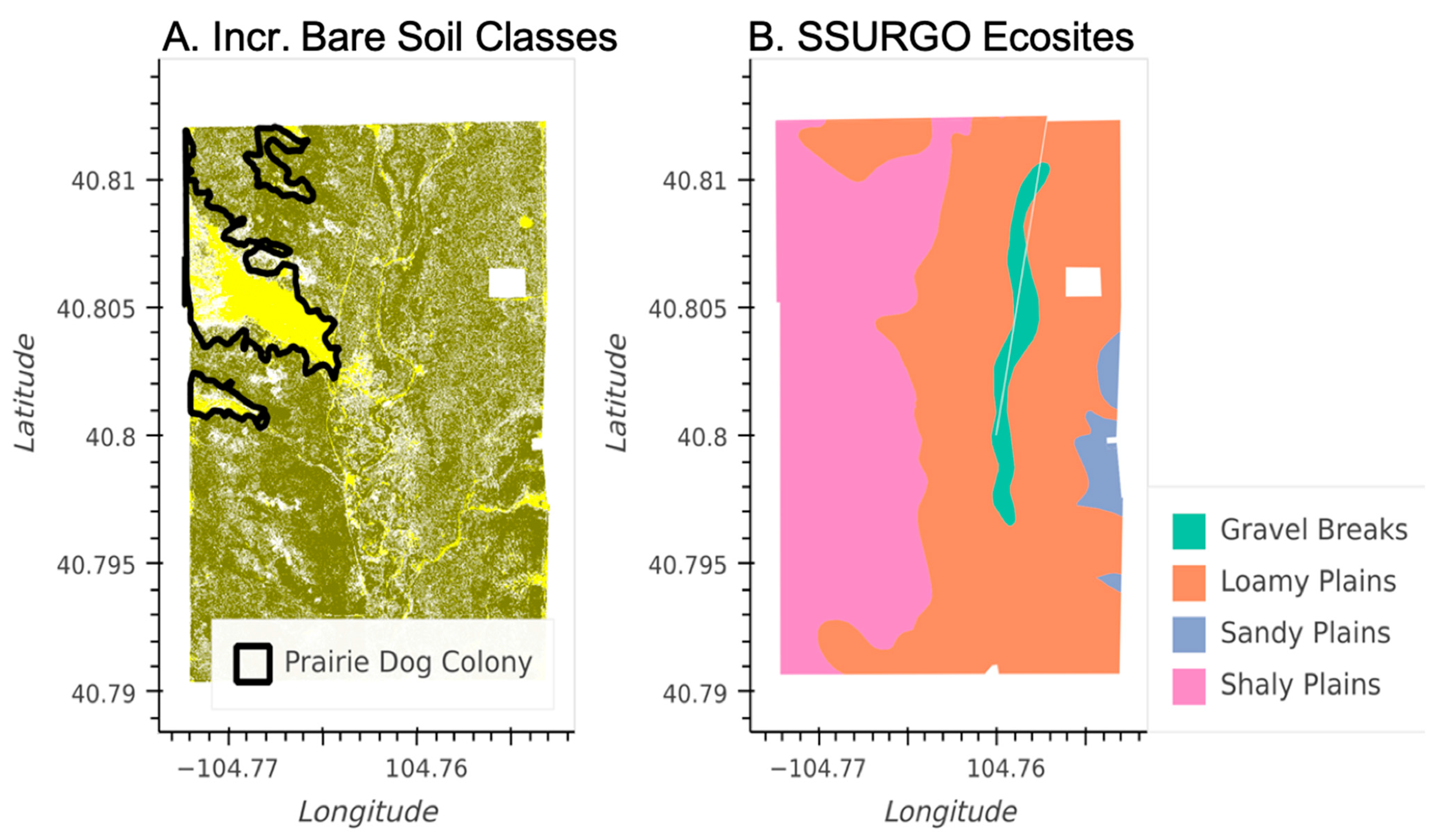
While overall plant community compositional shifts at CPER between 2013 and 2017 are likely related to climate dynamics, our plant community maps were also able to detect the effects of pasture-scale management and natural disturbances. Figure 9 shows the plant communities in 2013 that include elevated bare-soil components along with ground-based prairie dog colony perimeter maps from the current and previous years. The regions of elevated bare soil are strongly correlated to the regions that were actively occupied by prairie dogs in both 2012 and 2013. Furthermore, SSURGO, a static dataset that uses soils information to predict vegetation properties, was not able to detect the dynamic effects of the prairie dog colonies on the vegetation (Figure 9).
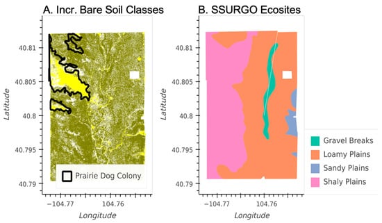
Figure 9.
Maps of a pasture at CPER (see Figure 1) with extensive prairie dog colonies. (A) 2013 NEON plant community classification map showing regions with elevated bare soil (yellow), regions with more continuous vegetation cover (olive), and boundaries indicating regions that had active prairie dog colonies during both 2012 and 2013 based on detailed in situ (field-based) mapping (black polygons). (B) SSURGO Ecosite map of the same pasture.
For the LTGI experiment, our plant community classification results match plot-based results [35] that found strong relationships between long-term grazing intensity and plant community composition. The plant community class map not only captures broad, pasture-scale trends related to grazing intensity (Figure 10), but also displays the finer-scale, spatially explicit heterogeneity present within each of the larger pastures. For example, grazing exclosures (dotted red boxes in Figure 10) are fenced areas within the pastures where cattle cannot graze, and these were established as experimental controls. Even within the moderately and heavily grazed pastures, these exclosures show a relative increase in the abundance of C3-dominated plant communities, congruent with previous ground-based measurements [47]. Additionally, bare soil patches caused by heavy cattle traffic around water tanks are visible in the lightly (northeast corner), moderately (northwest corner), and heavily (northwest corner) grazed pastures. Finally, the effects of topography on vegetation composition are also visible, particularly in the moderately grazed pasture; this type of topographically generated heterogeneity creates habitats for wildlife as well as patches of high-quality forage for livestock.
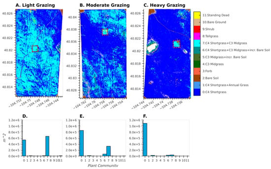
Figure 10.
Results of the 2017 plant community classification across three pastures at CPER (see Figure 1) with increasing levels of grazing (A–C) associated with the LTGI experiment. Dotted red polygons show grazing exclosures within each pasture. Associated with each map is a histogram (D–F) that shows the area of each plant community class for the above pasture.
4. Discussion
Our results show that airborne hyperspectral imaging has the potential to map grassland plant communities across relatively large areas at a fine spatial resolution. Mapping grassland dynamics at fine spatial and species resolutions is challenging due to the similar spectral profiles shared by ecologically distinct grasses, and these difficulties are exacerbated by sub-pixel-scale interference from standing dead vegetation and bare soil, as well as the very fine scale at which grasses, forbs, and shrubs are intermingled within the landscape [14]. The rich spectral information and relatively fine spatial resolution of the NEON AOP hyperspectral data were able to partially resolve these challenges by mapping vegetation at the plant community class scale, rather than the species level. Efforts to map individual grassland species suggest that pixel resolutions of <1 cm may be required to achieve satisfactory results [14], which is currently impractical for mapping large areas. Our community class-level approach allowed for the production of landscape-scale plant composition maps within a spectrally similar grassland context. Although these maps did not resolve the percent cover of each individual species, they were still able to provide very detailed, ecologically and management-relevant information on plant community composition at fine spatial scales. For systems where plants or other features are spectrally similar and highly intermixed at sub-pixel scales, we conclude that although spectral unmixing may be infeasible, a “community class” approach can provide a path forward for obtaining information-rich results.
Our modelling approach performed very well for some community classes and less well for others (see Figure 5). This result may have arisen, in part, from utilizing ground-based training/validation data that were collected at coarser spatial scales (25-m transects) than the NEON hyperspectral data (1 m). Transects were selected to represent each plant community class, but we were unable to quantify the spatial homogeneity of community composition within the inference region (a 2-m buffer) around each transect. For example, if a transect contained 50% C4 shortgrasses and 50% C3 midgrasses based on the ground-based LPI data, this could correspond to either (1) 100% of the 1 m pixels containing an even mixture of the two functional types, or (2) 50% of the pixels being dominated by C3 midgrasses, 50% of the pixels being dominated by C4 shortgrasses, and 0% containing an even mixture of the two functional types. Therefore, we suspect that a portion of pixels within the training transects likely differed from the plant community class to which they were assigned, resulting in sub-optimal training data and lower accuracies during validation. This may have especially been the case for plant communities containing a mixture of dominant and subdominant plant species (e.g., C4 shortgrasses mixed with C3 midgrasses), resulting in lower classification accuracies for these classes. In future years, we plan to develop more robust and homogeneous ROIs for training and validation. With better ROIs, we plan to explore the possibilities of further improvements to the classification pipeline, including potentially developing a species-level unmixing model for some of the more dominant plant species.
Annual variability in productivity and species composition made producing temporally consistent plant composition maps challenging. For example, transects sampled in 2013 that clustered into the C3 Midgrass community contained a lower mean cover of P. smithii than transects clustered into this community in 2017. Such dynamics can significantly complicate the robustness of models whose inference space is intended to include both spatially and temporally heterogeneous conditions [48]. Therefore, having a multi-year dataset that encompasses the full range of vegetation variability was critical to develop plant community classes that represented the true dynamics of the system. However, to ensure the temporal consistency of the model, it is preferable to develop training data that are collected in each year for which the calibration will be applied. We were able to accomplish this due to the extensive ground-based sampling conducted annually at CPER (>400 transects sampled per year) despite the overall shift in plant communities. The CPER transect data captured a large enough range in spatial plant community variability that we were able to identify transects in both 2013 and 2017 with consistent species composition for the majority of the plant community classes of interest. Using long-term data to document temporal shifts in plant community composition over broad spatial scales may be particularly important in the context of climate change adaptation.
Our analysis showed an increase in plant communities containing C3 midgrasses, predominantly P. smithii and H. comata, from 2013 to 2017. This shift is consistent with a gradual increase in these species documented during the 1980s through 2011 [35,47], and could have arisen both as a result of above-average precipitation during 2013–2017 as well as directional shifts associated with rising atmospheric CO2, which benefits the production of C3 midgrasses at this site [49]. We note that the study area experienced a prolonged period of above-average precipitation and below-average temperatures from late 2013 to 2015 (see Figure 1D). These conditions tend to stimulate the production of C3 midgrasses, which are less tolerant of heat and drought [7]. Additionally, an epizootic outbreak of plague (caused by the bacterium Yersinia pestis) affected three large prairie dog colonies within the study area in 2015 and 2016, substantially reducing their populations [50] and subsequently reducing their grazing of C3 midgrass.
In addition to documenting temporal shifts in community composition, case study results demonstrate several other potential applications of this type of approach. Plant community mapping can be used to document the effects of grazing management decisions or natural disturbances (burrowing mammals, fire) at a high spatial resolution across broad spatial extents that would be hard or impossible to sample using traditional plot-based sampling. Studies at smaller, pasture-scales, conducted over the past four decades examining how plant community composition affects cattle grazing distribution relied on detailed, ground-based maps [51,52], but with the use of remotely sensed data, mean that investigations can now be extended to a far wider range of conditions and spatial scales. In particular, combining high-resolution, landscape-scale vegetation maps with newly emerging technologies to control livestock movement, such as virtual fencing, will create a new era of opportunity to manage livestock across a far wider range of spatial scales than the pasture sizes currently imposed by existing fencing infrastructure [53].The wall-to-wall coverage offered by remotely sensed data not only allows for more accurate pasture-scale integration, but also allows for the identification of rare but potentially important features or trends within a given area of interest.
Furthermore, plant community maps can also improve other grassland mapping and modelling efforts when the response of the variable(s) of interest is dependent on plant species composition. For example, Magiera et al. [54] found that including a species composition map improved estimates of biomass yield from RapidEye satellite imagery in mountainous grasslands. Likewise, Gaffney et al. [48] found that regression coefficients differed for C3 vs. C4 dominated plots when modelling grassland productivity from satellite-derived absorbed photosynthetically active radiation (APAR).
5. Conclusions
In the era of big data and rapid global change, advanced programming and computing skills will be increasingly necessary to answer key questions about complex biological systems. In our study, the high resolution of the data posed challenges from a computational standpoint (e.g., >150 billion observations). Here, we presented a set of novel methodologies to preprocess, mosaic, and classify NEON AOP hyperspectral data across the CPER domain along with a computationally efficient python code, capable of processing the data and implementing a robust machine learning algorithm, in a distributed computing environment on a HPC system. The methods and computational approach outlined in this paper are transferable to other NEON domains, where researchers will be able to leverage AOP hyperspectral data, integrated to ground-based observations, to better characterize fine-scaled ecological processes. Our work highlights the importance and power of interdisciplinary approaches that link computational scientists with ecologists; such partnerships have the potential to rapidly advance our understanding of dynamic ecosystem patterns and processes at management-relevant spatial and temporal scales.
The plant community maps we generated for this shortgrass steppe landscape will advance research on the applications of precision livestock and wildlife management approaches that require an understanding of how grazers respond to fine-scale variation in vegetation dynamics at scales from hectares (e.g., individual drainages and hillslopes) to broad landscapes. Detailed plant community information could also revolutionize the ability of managers to apply precision vegetation management (e.g., management to increase or decrease the abundance or spatial extent of certain plant community classes) as well as spatially targeted conservation efforts for key wildlife habitat features embedded within vast rangeland landscapes.
Author Contributions
Conceptualization, D.J.A. and L.M.P.; Data curation, S.P.K.; Formal analysis, R.G., S.P.K. and L.M.P.; Funding acquisition, L.M.P.; Methodology, R.G., D.J.A., S.P.K. and L.M.P.; Project admin-istration, L.M.P.; Resources, L.M.P.; Software, R.G. and S.P.K.; Supervision, D.J.A.; Visualization, R.G.; Writing—original draft, R.G., D.J.A., S.P.K. and L.M.P.; Writing—review & editing, R.G., D.J.A., S.P.K. and L.M.P. All authors have read and agreed to the published version of the manuscript.
Funding
United States Department of Agriculture, Agricultural Research Service. This research was a contribution from the Long-Term Agroecosystem Research (LTAR) network. LTAR is supported by the United States Department of Agriculture.
Institutional Review Board Statement
Not applicable.
Informed Consent Statement
Not applicable.
Data Availability Statement
NEON hyperspectral data is publicly available from the NEON data portal (https://data.neonscience.org/, accessed on 4 November 2021). The field-based vegetation measurements across the CPER domain are publicly available on the USDA’s Ag Data Commons (https://data.nal.usda.gov/, accessed on 4 November 2021).
Acknowledgments
We thank Nick Dufek and numerous summer students for collecting the ground-based vegetation data, Nicole Kaplan for data management support, and Billy Armstrong for the initial exploratory work on this project. We thank the NEON AOP staff for fielding questions about the hyperspectral data and applying additional BRDF corrections to the data at our request.
Conflicts of Interest
The authors declare no conflict of interest.
References
- Irisarri, J.G.N.; Derner, J.D.; Porensky, L.M.; Augustine, D.J.; Reeves, J.L.; Mueller, K.E. Grazing Intensity Differentially Regulates ANPP Response to Precipitation in North American Semiarid Grasslands. Ecol. Appl. 2016, 26, 1370–1380. [Google Scholar] [CrossRef] [PubMed] [Green Version]
- Augustine, D.J.; McNaughton, S.J. Ungulate Effects on the Functional Species Composition of Plant Communities: Herbivore Selectivity and Plant Tolerance. J. Wildl. Manag. 1998, 62, 1165–1183. [Google Scholar] [CrossRef]
- Raynor, E.J.; Gersie, S.P.; Stephenson, M.B.; Clark, P.E.; Spiegal, S.A.; Boughton, R.K.; Bailey, D.W.; Cibils, A.; Smith, B.W.; Derner, J.D.; et al. Cattle Grazing Distribution Patterns Related to Topography Across Diverse Rangeland Ecosystems of North America. Rangel. Ecol. Manag. 2021, 75, 91–103. [Google Scholar] [CrossRef]
- Davis, S. Nest-Site Selection Patterns and the Influence of Vegetation on Nest Survival of Mixed-Grass Prairie Passerines. The Condor 2005, 107, 605–616. [Google Scholar] [CrossRef]
- Skagen, S.K.; Augustine, D.J.; Derner, J.D. Semi-arid Grassland Bird Responses to Patch-burn Grazing and Drought. J. Wildl. Manag. 2018, 82, 445–456. [Google Scholar] [CrossRef] [Green Version]
- Gao, Y.Z.; Giese, M.; Han, X.G.; Wang, D.L.; Zhou, Z.Y.; Brueck, H.; Lin, S.; Taube, F. Land Use and Drought Interactively Affect Interspecific Competition and Species Diversity at the Local Scale in a Semiarid Steppe Ecosystem. Ecol. Res. 2009, 24, 627–635. [Google Scholar] [CrossRef]
- Lauenroth, W. Vegetation of the Shortgrass Steppe. In Ecology of the Shortgrass Steppe: A Long-term Perspective; Lauenroth, W., Burke, I., Eds.; Oxford University Press: New York, NY, USA, 2008; pp. 70–83. [Google Scholar]
- McNaughton, S.J. Ecology of a Grazing Ecosystem: The Serengeti. Ecol. Monogr. 1985, 55, 259–294. [Google Scholar] [CrossRef]
- Milchunas, D.G.; Lauenroth, W.K.; Chapman, P.L.; Kazempour, M.K. Effects of Grazing, Topography, and Precipitation on the Structure of a Semiarid Grassland. Vegetatio 1989, 80, 11–23. [Google Scholar] [CrossRef]
- Peters, D.; Lauenroth, W.; Burke, I. The Role of Disturbances in Shortgrass Steppe Community and Ecosystem Dynamics. In Ecology of the Shortgrass Steppe: A Long-term Perspective; Lauenroth, W., Burke, I., Eds.; Oxford University Press: New York, NY, USA, 2008; pp. 84–118. [Google Scholar]
- Riginos, C.; Porensky, L.M.; Veblen, K.E.; Young, T.P. Herbivory and Drought Generate Short-Term Stochasticity and Long-Term Stability in a Savanna Understory Community. Ecol. Appl. Publ. Ecol. Soc. Am. 2018, 28, 323–335. [Google Scholar] [CrossRef] [PubMed] [Green Version]
- Jin, S.; Homer, C.; Yang, L.; Danielson, P.; Dewitz, J.; Li, C.; Zhu, Z.; Xian, G.; Howard, D. Overall Methodology Design for the United States National Land Cover Database 2016 Products. Remote Sens. 2019, 11, 2971. [Google Scholar] [CrossRef] [Green Version]
- Jones, M.O.; Allred, B.W.; Naugle, D.E.; Maestas, J.D.; Donnelly, P.; Metz, L.J.; Karl, J.; Smith, R.; Bestelmeyer, B.; Boyd, C.; et al. Innovation in Rangeland Monitoring: Annual, 30 m, Plant Functional Type Percent Cover Maps for U.S. Rangelands, 1984–2017. Ecosphere 2018, 9, e02430. [Google Scholar] [CrossRef]
- Lopatin, J.; Fassnacht, F.E.; Kattenborn, T.; Schmidtlein, S. Mapping Plant Species in Mixed Grassland Communities Using Close Range Imaging Spectroscopy. Remote Sens. Environ. 2017, 201, 12–23. [Google Scholar] [CrossRef]
- Porensky, L.; Derner, J.; Pellatz, D. Plant Community Responses to Historical Wildfire in a Shrubland-Grassland Ecotone Reveal Hybrid Disturbance Response. Ecosphere 2018, 8, e02363. [Google Scholar] [CrossRef] [Green Version]
- Duniway, M.; Bestelmeyer, B.; Tugel, A. Soil Processes and Properties That Distinguish Ecological Sites and States. Rangelands 2010, 32, 9–15. [Google Scholar] [CrossRef] [Green Version]
- Hoover, D.L.; Lauenroth, W.K.; Milchunas, D.G.; Porensky, L.M.; Augustine, D.J.; Derner, J.D. Sensitivity of Productivity to Precipitation Amount and Pattern Varies by Topographic Position in a Semiarid Grassland. Ecosphere 2021, 12, e03376. [Google Scholar] [CrossRef]
- Theron, E.; van Aardt, A.; du Preez, P. Vegetation Distribution along a Granite Catena, Southern Kruger National Park, South Africa. Koedoe 2020, 62, 11. [Google Scholar] [CrossRef]
- Jones, M.O.; Robinson, N.P.; Naugle, D.E.; Maestas, J.D.; Reeves, M.C.; Lankston, R.W.; Allred, B.W. Annual and 16-Day Rangeland Production Estimates for the Western United States. Rangel. Ecol. Manag. 2021, 77, 112–117. [Google Scholar] [CrossRef]
- Möckel, T.; Löfgren, O.; Prentice, H.C.; Eklundh, L.; Hall, K. Airborne Hyperspectral Data Predict Ellenberg Indicator Values for Nutrient and Moisture Availability in Dry Grazed Grasslands within a Local Agricultural Landscape. Ecol. Indic. 2016, 66, 503–516. [Google Scholar] [CrossRef]
- Pullanagari, R.R.; Kereszturi, G.; Yule, I. Integrating Airborne Hyperspectral, Topographic, and Soil Data for Estimating Pasture Quality Using Recursive Feature Elimination with Random Forest Regression. Remote Sens. 2018, 10, 1117. [Google Scholar] [CrossRef] [Green Version]
- Wang, Z.; Townsend, P.A.; Schweiger, A.K.; Couture, J.J.; Singh, A.; Hobbie, S.E.; Cavender-Bares, J. Mapping Foliar Functional Traits and Their Uncertainties across Three Years in a Grassland Experiment. Remote Sens. Environ. 2019, 221, 405–416. [Google Scholar] [CrossRef]
- Marcinkowska-Ochtyra, A.; Zagajewski, B.; Raczko, E.; Ochtyra, A.; Jarocińska, A. Classification of High-Mountain Vegetation Communities within a Diverse Giant Mountains Ecosystem Using Airborne APEX Hyperspectral Imagery. Remote Sens. 2018, 10, 570. [Google Scholar] [CrossRef] [Green Version]
- Rapinel, S.; Rossignol, N.; Hubert-Moy, L.; Bouzillé, J.-B.; Bonis, A. Mapping Grassland Plant Communities Using a Fuzzy Approach to Address Floristic and Spectral Uncertainty. Appl. Veg. Sci. 2018, 21, 678–693. [Google Scholar] [CrossRef]
- Kopeć, D.; Sabat-Tomala, A.; Michalska-Hejduk, D.; Jarocińska, A.; Niedzielko, J. Application of Airborne Hyperspectral Data for Mapping of Invasive Alien Spiraea Tomentosa, L.: A Serious Threat to Peat Bog Plant Communities. Wetl. Ecol. Manag. 2020, 28, 357–373. [Google Scholar] [CrossRef] [Green Version]
- Bradley, B.; Curtis, C.; Fusco, E.; Abatzoglou, J.; Balch, J.; Dadashi, S.; Tuanmu, M.-N. Cheatgrass (Bromus Tectorum) Distribution in the Intermountain Western United States and Its Relationship to Fire Frequency, Seasonality, and Ignitions. Biol. Invasions 2018, 20, 1493–1506. [Google Scholar] [CrossRef] [Green Version]
- Augustine, D.J.; Derner, J.D.; Fernández-Giménez, M.E.; Porensky, L.M.; Wilmer, H.; Briske, D.D. Adaptive, Multipaddock Rotational Grazing Management: A Ranch-Scale Assessment of Effects on Vegetation and Livestock Performance in Semiarid Rangeland. Rangel. Ecol. Manag. 2020, 73, 796–810. [Google Scholar] [CrossRef]
- Herrick, J.; Zee, J.V.; Havstad, K.; Burkett, L.M.; Whitford, W. Monitoring Manual for Grassland, Shrubland and Savanna Ecosystems. Methods and Interpretation; Jornada Experimental Range: Las Cruces, NM, USA, 2005; Volume 1. [Google Scholar]
- Karpowicz, B.; Kampe, T. NEON Imaging Spectrometer Radiance to Reflectance Algorithm Theoretical Basis Document; The National Ecological Observatory Network: Boulder, CO, USA, 2015. [Google Scholar]
- Liu, N.; Chlus, A.; Townsend, P.A. HyToolsPro: An Open Source Package for Pre-Processing Airborne Hyperspectral Images. In Proceedings of the AGU Fall Meeting 2019, San Francisco, CA, USA, 9–13 December 2019. [Google Scholar]
- Daughtry, C.S.T.; Doraiswamy, P.C.; Hunt, E.R.; Stern, A.J.; McMurtrey, J.E.; Prueger, J.H. Remote Sensing of Crop Residue Cover and Soil Tillage Intensity. Soil Tillage Res. 2006, 91, 101–108. [Google Scholar] [CrossRef]
- Guerschman, J.P.; Hill, M.J.; Renzullo, L.J.; Barrett, D.J.; Marks, A.S.; Botha, E.J. Estimating Fractional Cover of Photosynthetic Vegetation, Non-Photosynthetic Vegetation and Bare Soil in the Australian Tropical Savanna Region Upscaling the EO-1 Hyperion and MODIS Sensors. Remote Sens. Environ. 2009, 113, 928–945. [Google Scholar] [CrossRef]
- Pedregosa, F.; Varoquaux, G.; Gramfort, A.; Michel, V.; Thirion, B.; Grisel, O.; Blondel, M.; Prettenhofer, P.; Weiss, R.; Dubourg, V.; et al. Scikit-Learn: Machine Learning in Python. Mach. Learn. Python 2011, 12, 2825–2830. [Google Scholar]
- Klipple, G.E.; Costello, D.F. Vegetation and Cattle Responses to Different Intensities of Grazing on Short-Grass Ranges on Tlie Central Great Plains; US Department of Agriculture: Washington, DC, USA, 1960. [Google Scholar]
- Porensky, L.M.; Derner, J.D.; Augustine, D.J.; Milchunas, D.G. Plant Community Composition After 75 Yr of Sustained Grazing Intensity Treatments in Shortgrass Steppe. Rangel. Ecol. Manag. 2017, 70, 456–464. [Google Scholar] [CrossRef]
- Augustine, D.J.; Derner, J.D.; Detling, J.K. Testing for Thresholds in a Semiarid Grassland: The Influence of Prairie Dogs and Plague. Rangel. Ecol. Manag. 2014, 67, 701–709. [Google Scholar] [CrossRef]
- Hart, R.H.; Mary, M. Ashby Grazing Intensities, Vegetation, and Heifer Gains: 55 Years on Shortgrass. J. Range Manag. 1998, 51, 392–398. [Google Scholar] [CrossRef] [Green Version]
- Merkel, D. Docker: Lightweight Linux Containers for Consistent Development and Deployment. Linux J. 2014, 239, 2. [Google Scholar]
- Kluyver, T.; Ragan-Kelley, B.; Pérez, F.; Bussonnier, M.; Frederic, J.; Hamrick, J.; Grout, J.; Corlay, S.; Ivanov, P.; Abdalla, S.; et al. Jupyter Notebooks—A Publishing Format for Reproducible Computational Workflows. In Proceedings of the 20th International Conference on Electronic Publishing, Toronto, ON, Canada, 1 January 2016. [Google Scholar]
- Gaffney, R. Rmg55/Container_stacks: Dsir_2021.04.1; CERN: Meyrin, Switzerland, 2021. [Google Scholar]
- Dask Development Team. Dask: Library for Dynamic Task Scheduling; VMware Inc.: Palo Alto, CA, USA, 2016. [Google Scholar]
- Rocklin, M. Dask: Parallel Computation with Blocked Algorithms and Task Scheduling. In Proceedings of the 14th Python in Science Conference, Austin, TX, USA, 6–12 July 2015; pp. 126–132. [Google Scholar]
- Hoyer, S.; Hamman, J.J. Xarray: N-D Labeled Arrays and Datasets in Python. J. Open Res. Softw. 2017, 5, 10. [Google Scholar] [CrossRef] [Green Version]
- Bednar, J.A.; Crail, J.; Crist-Harif, J.; Rudiger, P.; Brener, G.; B, C.; Mease, J.; Signell, J.; Stevens, J.-L.; Collins, B.; et al. Holoviz/Datashader: Version 0.12.1; Zenodo: Meyrin, Switzerland, 2021. [Google Scholar]
- Rudiger, P.; Signell, J.; Bednar, J.A.; Andrew; Stevens, J.-L.; B, C.; Kbowen; Fast, T.; Graser, A.; AurelienSciarra; et al. Holoviz/Hvplot: Version 0.7.1; Zenodo: Meyrin, Switzerland, 2021. [Google Scholar]
- Rudiger, P.; Stevens, J.-L.; Bednar, J.A.; Nijholt, B.; Mease, J.; Andrew; B, C.; Randelhoff, A.; Tenner, V.; Maxalbert; et al. Holoviz/Holoviews: Version 1.14.3; Zenodo: Meyrin, Switzerland, 2021. [Google Scholar]
- Augustine, D.J.; Derner, J.D.; Milchunas, D.; Blumenthal, D.; Porensky, L.M. Grazing Moderates Increases in C3 Grass Abundance over Seven Decades across a Soil Texture Gradient in Shortgrass Steppe. J. Veg. Sci. 2017, 28, 562–572. [Google Scholar] [CrossRef]
- Gaffney, R.; Porensky, L.; Gao, F.; Irisarri, J.; Durante, M.; Derner, J.; Augustine, D. Using APAR to Predict Aboveground Plant Productivity in Semi-Aid Rangelands: Spatial and Temporal Relationships Differ. Remote Sens. 2018, 10, 1474. [Google Scholar] [CrossRef] [Green Version]
- Milchunas, D.G.; Mosier, A.R.; Morgan, J.A.; LeCain, D.R.; King, J.Y.; Nelson, J.A. Elevated CO2 and Defoliation Effects on a Shortgrass Steppe: Forage Quality versus Quantity for Ruminants. Agric. Ecosyst. Environ. 2005, 111, 166–184. [Google Scholar] [CrossRef]
- Augustine, D.J.; Derner, J.D. Long-Term Effects of Black-Tailed Prairie Dogs on Livestock Grazing Distribution and Mass Gain. J. Wildl. Manag. 2021, 85, 1332–1343. [Google Scholar] [CrossRef]
- Gersie, S.P.; Augustine, D.J.; Derner, J.D. Cattle Grazing Distribution in Shortgrass Steppe: Influences of Topography and Saline Soils. Rangel. Ecol. Manag. 2019, 72, 602–614. [Google Scholar] [CrossRef]
- Senft, R.L.; Rittenhouse, L.R.; Woodmansee, R.G. Factors Influencing Patterns of Cattle Grazing Behavior on Shortgrass Steppe. J. Range Manag. 1985, 38, 82. [Google Scholar] [CrossRef]
- Swain, D.L.; Charters, S.M. Back to Nature With Fenceless Farms—Technology Opportunities to Reconnect People and Food. Front. Sustain. Food Syst. 2021, 5, 222. [Google Scholar] [CrossRef]
- Magiera, A.; Feilhauer, H.; Waldhardt, R.; Wiesmair, M.; Otte, A. Modelling Biomass of Mountainous Grasslands by Including a Species Composition Map. Ecol. Indic. 2017, 78, 8–18. [Google Scholar] [CrossRef]


Publisher’s Note: MDPI stays neutral with regard to jurisdictional claims in published maps and institutional affiliations. |
© 2021 by the authors. Licensee MDPI, Basel, Switzerland. This article is an open access article distributed under the terms and conditions of the Creative Commons Attribution (CC BY) license (https://creativecommons.org/licenses/by/4.0/).