
The Salinity Pilot-Mission Exploitation Platform (Pi-MEP): A Hub for Validation and Exploitation of Satellite Sea Surface Salinity Data

 , , , , ,
Abstract
:1. Introduction
2. Datasets
2.1. In Situ SSS Datasets
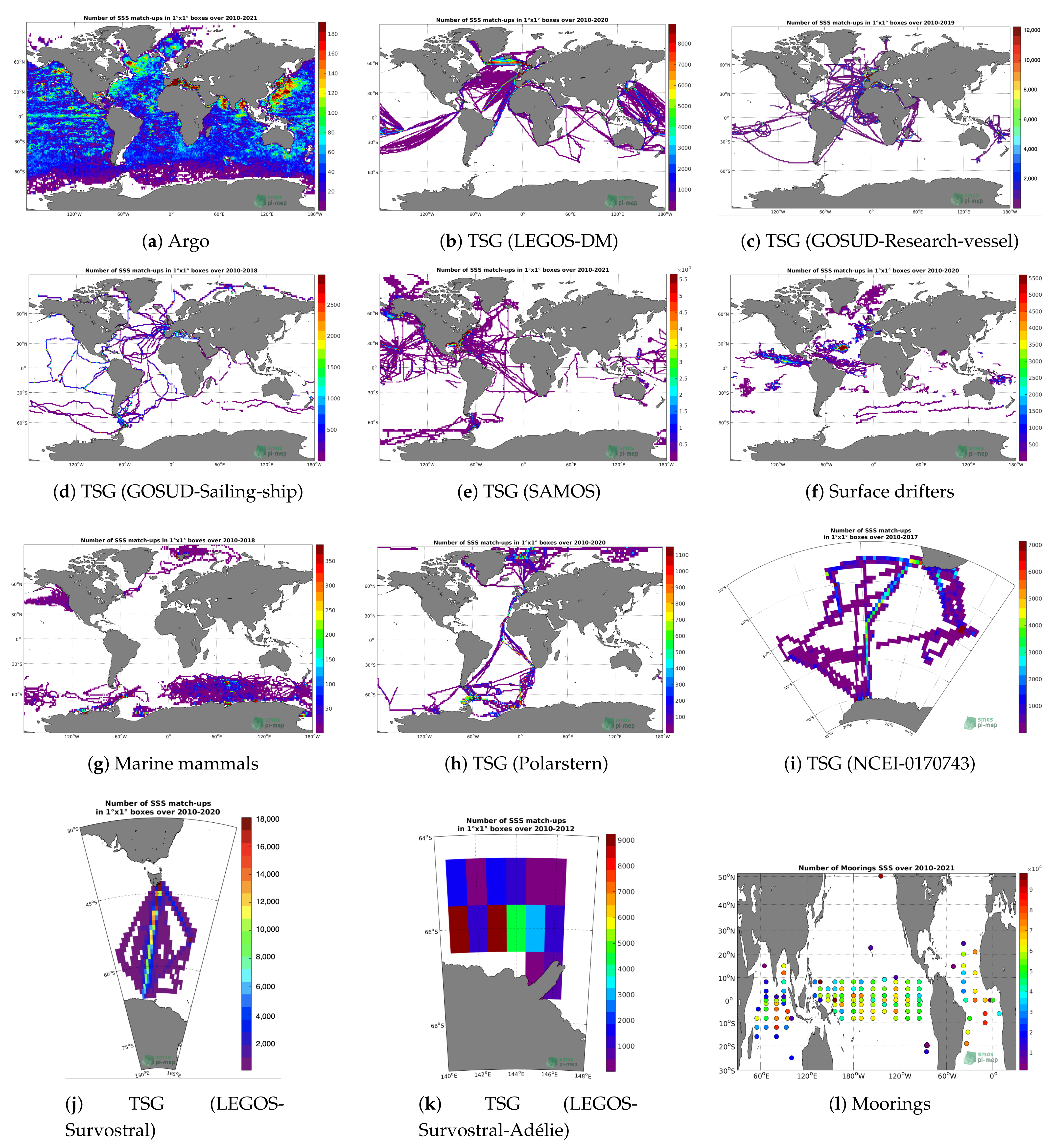
2.1.1. Argo
2.1.2. Thermosalinograph Dataset
- The TSG (LEGOS-DM) dataset corresponds to sea surface salinity delayed mode data derived from sensors on board voluntary observing ships (VOS). These data are collected, validated, archived, and made freely available by the French Sea Surface Salinity Observation Service [9]. Adjusted values (if available) and only collected TSG data that exhibit quality flags = 1 and 2 were used.
- The TSG (GOSUD-Research-vessel) dataset corresponds to French research vessels’ SSS data that have been collected since early 2000 as a contribution to the Global Ocean Surface Underway Data (GOSUD) program. The set of homogeneous instruments is permanently monitored and regularly calibrated. Water samples are taken on a daily basis by the crew and later analyzed in the laboratory. The careful calibration and instrument maintenance, complemented with a rigorous adjustment on water samples, lead an accuracy of a few 10 PSS in salinity. This delayed mode dataset is updated annually and freely available [10]. Adjusted values when available and only collected TSG data that exhibit quality flags 1 or 2 were used.
- The TSG (GOSUD-Sailing-ship) dataset corresponds to observations of sea surface salinity obtained from voluntary sailing ships using medium- or small-sized sensors. They complement the networks installed on research vessels or commercial ships. This delayed mode dataset [11] is updated annually as a contribution to GOSUD (http://www.gosud.org, accessed on 30 April 2021) and freely available. Adjusted values when available and only collected TSG data that exhibit quality flags = 1 and 2 were used.
- The TSG (SAMOS) dataset corresponds to “Research” quality data from the US Shipboard Automated Meteorological and Oceanographic System (SAMOS) initiative [12]. Data are available at http://samos.coaps.fsu.edu/html/ and has been accessed on 30 April 2021. Adjusted values when available and only collected TSG data that exhibit quality flags = 1 and 2 were used. After visual inspection, data from the NANCY FOSTER (ID = “WTER”, IMO = “008993227”) acquired on 21 March 2011 and all data from the ATLANTIS (ID = “KAQP”, IMO = “009105798”) for the year 2010 have been removed from this dataset.
- The TSG (LEGOS-Survostral) dataset corresponds to delayed mode regional data from the TSG installed on the Astrolabe vessel (IPEV) during the round trips between Hobart (Tasmania) and the French Antarctic base at Dumont d’Urville [13]. It is provided by the Survostral project (http://www.legos.obs-mip.fr/projets/chantiers-geographiques/zones-polaires-glaciers/survostral/) and has been accessed at ftp://ftp.legos.obs-mip.fr/pub/soa/salinite/survostral/dmdataadelie2003ongoing/, accessed on 30 April 2021. Adjusted values when available and only collected TSG data that exhibit quality flags = 1 and 2 were used.
- The TSG (LEGOS-Survostral-Adélie) dataset corresponds to delayed mode regional data along the Adélie coast provided by the Survostral projectand has been accessed at ftp://ftp.legos.obs-mip.fr/pub/soa/salinite/survostral/dmdataadelie2003ongoing/, accessed on 30 April 2021. Adjusted values when available and only collected TSG data that exhibit quality flags = 1 and 2 were used.
- The TSG (Polarstern) dataset has been gathered through the https://www.pangaea.de/ data warehouse utility accessed on 30 April 2021 using the following criteria: basis: “Polarstern”, device: “Underway cruise track measurements (CT)”, time coverage from 1 January 2010 to present. The result of the query is a collection of 79 different datasets.
- The TSG (NCEI-0170743) dataset [14] contains sea surface temperature (SST) and salinity data collected from 2010 to 2017 in the South Atlantic Ocean and Southern Ocean from S.A. Agulhas and Agulhas-II research vessels, in the framework of South African National Antarctic Programme (SANAP), South African Department of Environmental Affairs (DEA) and Italian National Antarctic Research Programme (PNRA) scientific activities. Measurements were obtained through thermosalinographs (TSG) over several cruises to both Antarctica and sub-Antarctic islands. On-board TSG devices were regularly calibrated and continuously monitored in between cruises; no appreciable sensor drift emerged. Independent water samples taken along the cruises were used to validate the data; salinity measurement error was a few hundredths of a unit on the practical salinity scale. A careful quality control allowed us to discard erroneous data for each single campaign.
2.1.3. Surface Drifters
2.1.4. Marine Mammals
2.1.5. Moorings
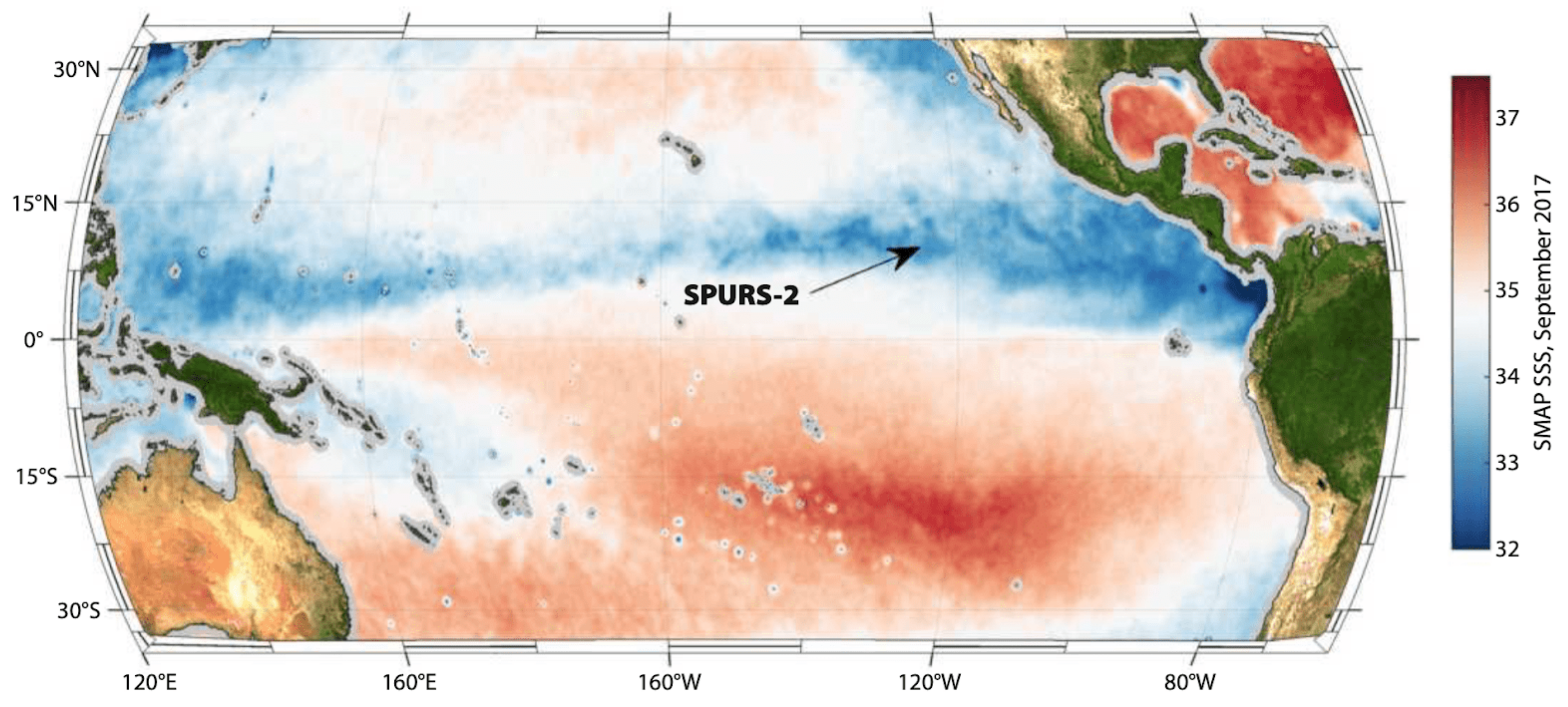
2.1.6. SPURS-2 Field Campaign Datasets
- The Waveglider is an autonomous platform propelled by the conversion of ocean wave energy into forward thrust and employs solar panels to power instrumentation. For SPURS-2, sensors included a CTD at the near surface and another at 6 m depth, providing continuous salinity and temperature observations plus air temperature and wind measurements. Three wavegliders (https://doi.org/10.5067/SPUR2-GLID3, accessed on 30 April 2021) were deployed from the R/V Revelle in August 2016 and again in November 2017 before final retrieval at the conclusion of the second cruise. Waveglider trajectories followed a 20 × 20 km square loop around the moorings and a butterfly pattern around the neutrally buoyant float.
- The Seaglider is an autonomous profiler measuring salinity and temperature. A total of five Seagliders (https://doi.org/10.5067/SPUR2-GLID1, accessed on 30 April 2021) were deployed over the two SPURS-2 cruises. Three Seagliders were deployed on the first R/V Revelle cruise in August 2016, recovered by the Lady Amber after 7 months and redeployed, to be retrieved finally during the second cruise in November 2017. One of the Seagliders was deployed alongside the Lagrangian array and tracked it across the study region, diving to depths of 1000 m.
- The Salinity Snake (SS) measures sea surface salinity in the top 1–2 cm of the water column, which is the radiometric depth of L-Band satellite radiometers such as on Aquarius/SAC-D, SMAP and SMOS satellites, which measure salinity remotely. The SS consists of four key components: a 10 m boom mast, a hose, which is deployed from this boom, a powerful self-priming peristaltic pump, which transports a constant stream of a seawater/air emulsion, and a shipboard apparatus, which filters, de-bubbles, sterilizes and analyzes the salinity of the water. The SS (https://doi.org/10.5067/SPUR2-SNAKE, accessed on 30 April 2021) was deployed during both SPURS-2 R/V Revelle cruises in August 2016 and October 2017.
- Saildrone is a state-of-the-art, remotely guided, wind- and solar-powered unmanned surface vehicle (USV) capable of long-distance deployments lasting up to 12 months. It is equipped with a suite of instruments and sensors providing high-quality, georeferenced, near-real-time, multiparameter surface ocean and atmospheric observations while transiting at typical speeds of 3–5 knots. Two saildrones (https://doi.org/10.5067/SPUR2-SDRON, accessed on 30 April 2021) were deployed over a month period during the second SPURS-2 R/V Revelle cruise in 2017. The SPURS-2 campaign involved two month-long cruises by the R/V Revelle in August 2016 and October 2017 combined with complementary sampling on a more continuous basis over this period by the schooner Lady Amber.
2.1.7. In Situ SSS Analyses and Climatologies
- The In Situ Analysis System (ISAS), as described in [7], is an optimal interpolation tool developed and run at the Laboratory for Ocean Physics and Satellite remote sensing (LOPS) in close collaboration with Coriolis. It was initially designed to synthetize the temperature and salinity profiles collected by the ARGO program. It has been later extended to accommodate all types of vertical profiles as well as time series. The products used are the INSITU_GLO_TS_OA_REP_OBSERVATIONS_013_002_b for the period 2010 to June 2020 and the INSITU_GLO_TS_OA_NRT_OBSERVATIONS_013_002_a for the near-real-time observations (2020–2021) provided by the Copernicus Marine Environment Monitoring Service (http://marine.copernicus.eu/, accessed on 30 April 2021). For the purposes of validation, the ISAS monthly SSS fields (spatial resolution of 0.5× 0.5) at 5 m depth were collocated and compared with the satellite SSS products and further included in the Pi-MEP match-up files.
- The new version of the Roemmich-Gilson Argo Climatology as described in [18] and provided by Scripps Institution of Oceanography was also used.
- Global gridded salinity field produced by the variational interpolation from Argo profiles provided by the IPRC are also ingested by the platform.
- The World Ocean Atlas (WOA) is a set of objectively analyzed climatological fields of in situ temperatures, salinity and other variables provided at standard depth levels for annual, seasonal, and monthly compositing periods for the World Ocean. Salinity fields at the surface and 1 resolution grid are used as a complement to the ISAS to characterize the climatological components (annual, monthly and standard deviation) at the match-up pairs’ locations and dates.
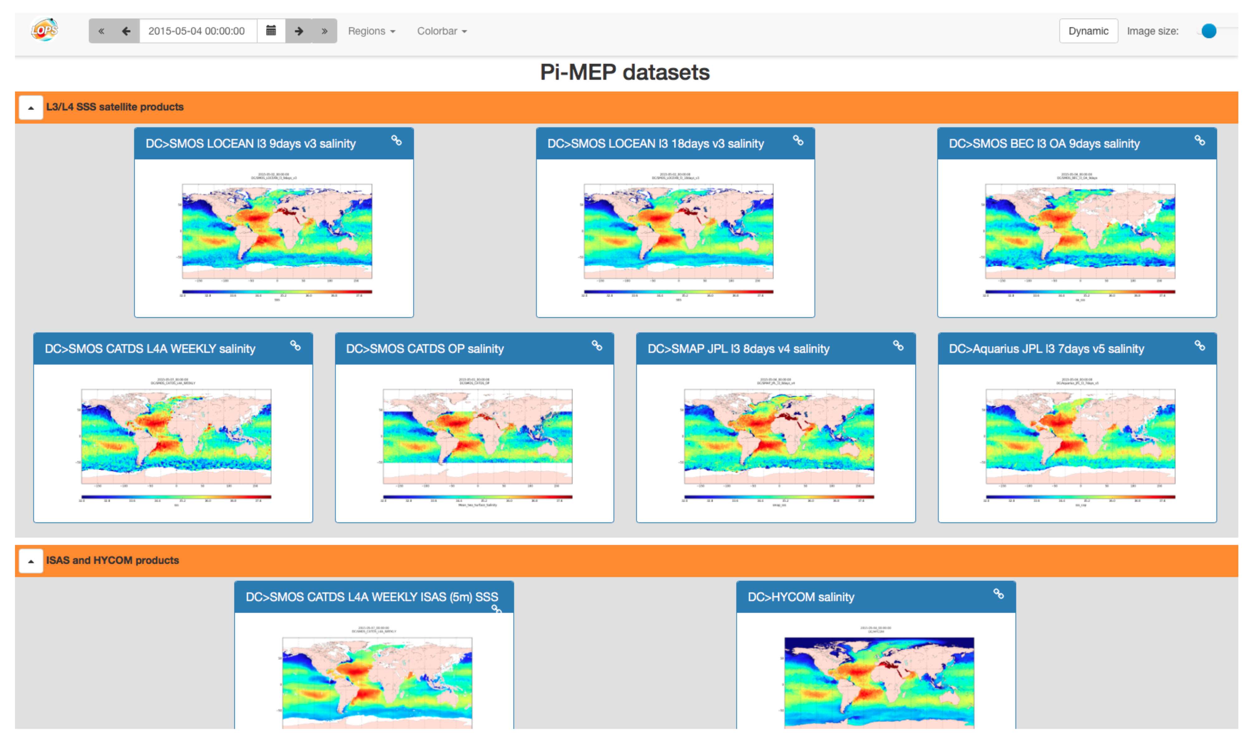
2.2. SSS Satellite Products
- Level 2: swath SSS data (50-minute half orbit for SMOS, and 98-minute orbit for SMAP and Aquarius);
- Level 3: space-time SSS composite of one single sensor swath data;
- Level 4: space-time SSS composite of multisensor SSS data.
2.3. Thematic Datasets
2.3.1. Precipitation
2.3.2. Surface Wind Speed
- The Advanced SCATterometer (ASCAT) daily wind speed produced and made available at Ifremer/CERSAT on a 0.25× 0.25 resolution grid [21].
- The Cross-Calibrated Multi-Platform (CCMP V2.0) gridded surface vector winds produced using satellite, moored buoys, and model wind data, available from Remote Sensing Systems (http://www.remss.com/measurements/ccmp/, accessed on 30 April 2021). The V2 CCMP processing combines Version-7 RSS radiometer wind speeds, QuikSCAT and ASCAT scatterometers wind vectors, moored buoy wind data, and ERA-Interim model wind fields using a variational analysis method (VAM) to produce four maps daily of 0.25 gridded vector winds.
- The Global Blended Mean Wind Fields, produced by Ifremer and distributed by CMEMS (http://marine.copernicus.eu/ with product identifierWIND_GLO_WIND_L4_REP_OBSERVATIONS_012_006, accessed on 30 April 2021), include wind stress components (meridional and zonal), and wind modules. The analysis was performed for each synoptic time (00h:00; 06h:00; 12h:00; 18h:00 UTC) and with a spatial resolution of 0.25 in longitude and latitude over the global ocean.
2.3.3. Sea Surface Temperature
- The Group for High-Resolution Sea Surface Temperature (GHRSST) global Level 4 sea surface temperature analysis produced daily on a 0.25-degree grid at the NOAA National Centers for Environmental Information. This product uses optimal interpolation (OI) by interpolating and extrapolating SST observations from different sources, resulting in a smoothed complete field. The sources of data are satellite (AVHRR) and in situ platforms (i.e., ships, buoys, and Argo floats above 5 m depth), and the specific datasets employed may change over time. In the regions with sea-ice concentrations higher than 30%, the freezing points of seawater are used to generate proxy SSTs. A preliminary version of this file is produced in near-real time (1-day latency), and then replaced with a final version after 2 weeks. The v2.1 is updated via the AVHRR_OI-NCEI-L4-GLOB-v2.0 data. Major improvements include: (1) in situ ship and buoy data changed from the NCEP Traditional Alphanumeric Codes (TAC) to the NCEI merged TAC + Binary Universal Form for the Representation (BUFR) data, with a large increase in buoy data included to correct satellite SST biases; (2) the addition of Argo float-observed SST data as well, for further correction of satellite SST biases; (3) satellite input from the METOP-A and NOAA-19 to METOP-A and METOP-B, removing degraded satellite data; (4) revised ship-buoy SST corrections for improved accuracy; and (5) Revised sea-ice-concentration to SST conversion to remove warm biases in the Arctic region [22]. These updates only apply to granules after 1 January 2016. The data pre 2016 are still the same as v2.0 except for metadata upgrades.
- Another (GHRSST) Level 4 SST analysis produced daily on an operational basis at the UK Met Office using OI on a global 0.054 degree grid is also used to obtain higher spatial resolution SST information (subpixel variability). The Operational Sea Surface Temperature and Sea Ice Analysis (OSTIA) analysis uses satellite data from sensors that include the Advanced Very High Resolution Radiometer (AVHRR), the Advanced Along Track Scanning Radiometer (AATSR), the Spinning Enhanced Visible and Infrared Imager (SEVIRI), the Advanced Microwave Scanning Radiometer-EOS (AMSRE), the Tropical Rainfall Measuring Mission Microwave Imager (TMI), and in situ data from drifting and moored buoys. This analysis has a highly smoothed SST field and was specifically produced to support SST data assimilation into Numerical Weather Prediction (NWP) models.
2.3.4. Models and Assimilation
- the operational Mercator global ocean analysis and forecast system at 1/12 degree of daily mean salinity field at surface over the global ocean as provided by CMEMS (https://resources.marine.copernicus.eu/products with product identifier GLOBAL_ANALYSIS_FORECAST_PHY_001_024 accessed on 30 April 2021)
- the Global Analysed Sea Surface Salinity and Density [23] as provided by CMEMS (https://resources.marine.copernicus.eu/products with product identifier MULTIOBS_GLO_PHY_REP_015_002 accessed on 30 April 2021)
- the Sea Surface Salinity from GLORYS12V1, the CMEMS global ocean eddy-resolving (1/12 horizontal resolution, 50 vertical levels) reanalysis, as provided by CMEMS (https://resources.marine.copernicus.eu/products with product identifierGLOBAL_REANALYSIS_PHY_001_030 accessed on 30 April 2021).
- the Daily HYCOM+NCODA Global 1/12 Analysis salinity field interpolated on a uniform 0.08 degree lat/lon grid between 80.48S and 80.48N (GLBu0.08). HYCOM is a data-assimilative hybrid isopycnal-sigma-pressure (generalized) coordinate ocean model (called HYbrid Coordinate Ocean Model). It uses the Navy Coupled Ocean Data Assimilation (NCODA) system [24,25] for data assimilation. NCODA uses the model forecast for a first estimate in a 3D variational scheme and assimilates available satellite altimeter observations (along the track obtained via the NAVOCEANO Altimeter Data Fusion Center), satellite and in situ SST as well as available in situ vertical temperature and salinity profiles from XBTs, Argo floats and moored buoys. MODAS synthetics are used for the downward projection of surface information [26].
- ECCO Version 4 Release 3 (V4r3), covering the period 1992–2015, an ocean state estimate of the Consortium for Estimating the Circulation and Climate of the Ocean (ECCO) [27,28], which synthesizes nearly all modern observations with an ocean circulation model (MITgcm, originally described by [29]) into coherent, physically consistent descriptions of the ocean’s time-evolving state covering the era of satellite altimetry.
2.3.5. Other Auxiliary Datasets
- Zonal and meridional components of the surface geostrophic current and the Ekman current at 15 m depth from GlobCurrent. The data are interpolated and collocated to a common grid with a spatial resolution of 25 km and a temporal resolution of 1 day for the geostrophic current and three hours for the Ekman currents.
- The evaporation rate from the OAFlux project determined from the relation: Evaporation = latent heat flux / , where is the density of sea water, and is the latent heat of vaporization that can be expressed as (ftp://ftp.whoi.edu/pub/science/oaflux/datav3/daily/evaporation/, accessed on 30 April 2021)
- Modis 8-day colored dissolved and detrital organic materials (CDOM) and chlorophyll concentration (CHL1) provided by the GlobColour project (https://www.globcolour.info/, accessed on 30 April 2021).
- Global sea-ice concentration interim climate data recorded from 2016 onwards (v2.0, OSI-430-b) and OSI-450, from 2010 to 2015, provided by OSI SAF (http://www.osi-saf.org/?q=content/sea-ice-products, accessed on 30 April 2021).
- Multimission altimeter satellite gridded sea level anomalies (SLA) computed with respect to a twenty-year mean (1993–2012) and using an optimal and centered computation time window (6 weeks before and after the date). This product is processed by the SL-TAC multimission altimeter data processing system and distributed by CMEMS (https://resources.marine.copernicus.eu/products with product identifier SEALEVEL_GLO_PHY_L4_REP_OBSERVATIONS_008_047 andSEALEVEL_GLO_PHY_L4_NRT_OBSERVATIONS_008_046 accessed on 30 April 2021.
- ETOPO-1 is a 1 arc-minute global relief model of Earth’s surface that integrates land topography and ocean bathymetry [30].
- Baroclinic Rossby radius of deformation from [31].
3. Validation: Match-Up Generation and Processing
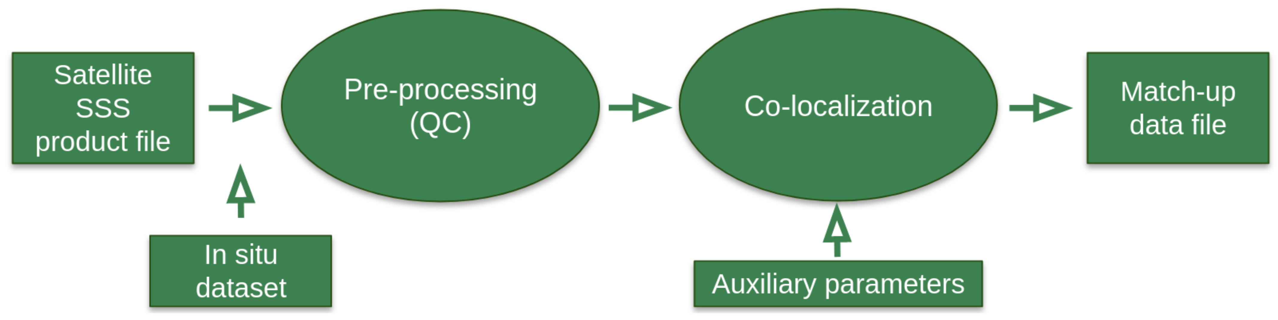
3.1. Overview of the Match-Up Generation Method
- The preparation of the input in situ and satellite data.
- The co-localization of satellite products with in situ SSS measurements.
- The co-localization of the in situ/satellite pair with auxiliary geophysical information.
3.1.1. In Situ/Satellite Data Preprocessing
3.1.2. In Situ/Satellite Co-Localization
- For L2 SSS swath data:If is the spatial resolution of the satellite swath SSS product, for each in situ data sample collected in the Pi-MEP database, the platform searches for all satellite SSS data found at grid nodes located within a radius of /2 from the in situ data location and acquired with a time-lag from the in situ measurement date that is less than or equal to ± 12 h. If several satellite SSS samples are found to meet these criteria, the final satellite SSS match-up point is selected to be the closest in time from the in situ data measurement date. The final spatial and temporal lags between the in situ and satellite data are stored in the MDB files.
- For L3 and L4 composite SSS products:If is the spatial resolution of the composite satellite SSS product and D the period over which the composite product was built (e.g., periods of 1, 7, 8, 9, 10, 18 days, 1 month, etc.) with central time , for each in situ data sample collected in the Pi-MEP database during the time interval [, ], the platform searches for all satellite SSS data of the composite product found at grid nodes located within a radius of /2 from the in situ data location. If several satellite SSS product samples are found to meet these criteria, the final satellite SSS match-up point is chosen to be the composite SSS with central time which is the closest in time from the in situ data measurement date. The final spatial and temporal lags between the in situ and satellite data are stored in the MDB files.
3.1.3. MDB Pair Co-Localization with Auxiliary Data and Complementary Information
- The ASCAT wind speed product of the same day found at the ASCAT 1/4 grid node that is closest to the in situ data location. We then store the time series of the ASCAT wind speed at the same node for the 10 days prior to the in situ measurement day.
- If the in situ data are located within the 60N–60S band, we select the CMORPH 3-hourly product that is closest in time from and found at the CMORPH 1/4 grid node that is the closest distance from the in situ data location. We then store the time series of the CMORPH rain rate at the same node for 10 days prior to the in situ measurement time.
- The vertical distribution of pressure at which the profiles were measured;
- The vertical S(z) and T(z) profiles;
- The vertical potential density anomaly profile ;
- The mixed layer depth (MLD). The MLD is defined here as the depth where the potential density has increased from the reference depth (10 meter) by a threshold equivalent to 0.2 C decrease in temperature at constant salinity: with , where and are the temperature and salinity at the reference depth (i.e., 10 m) [32,33];
- The top of the thermocline depth (TTD) is defined as the depth at which temperature decreases from its 10 m-depth value by 0.2 C;
- The barrier layer thickness (BLT) is defined as the difference between the MLD and the TTD. If BLT < 0, it corresponds to a vertically density compensated layer whose thickness is then the absolute value of (TTD-MLD);
- The vertical profile of the buoyancy frequency .
3.2. Match-Up Characteristics for Each Specific In Situ/Satellite Pair
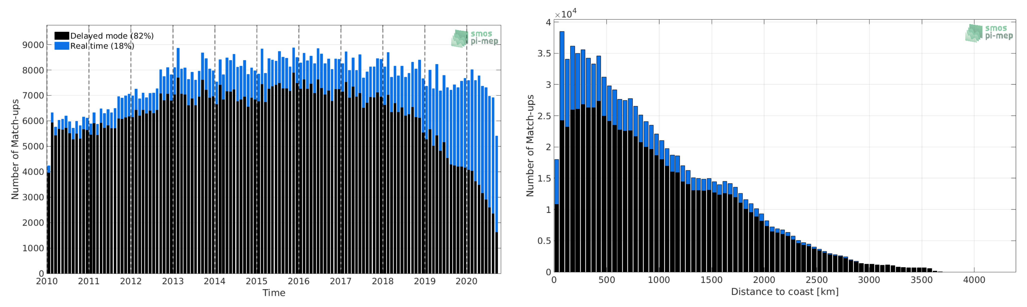
3.2.1. Number of Paired SSS Data as a Function of Time and Distance to Coast
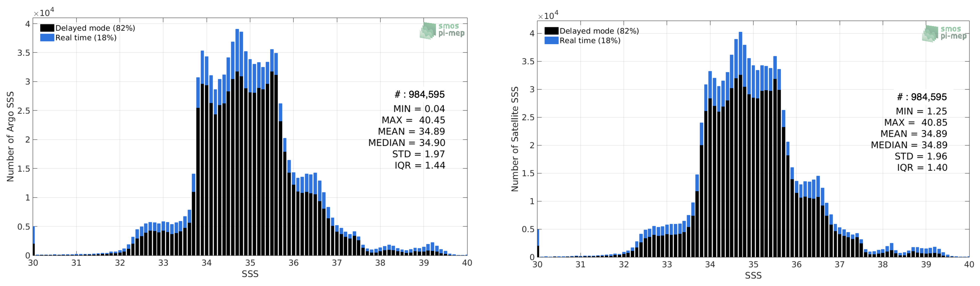
3.2.2. Histograms of the SSS Match-Ups
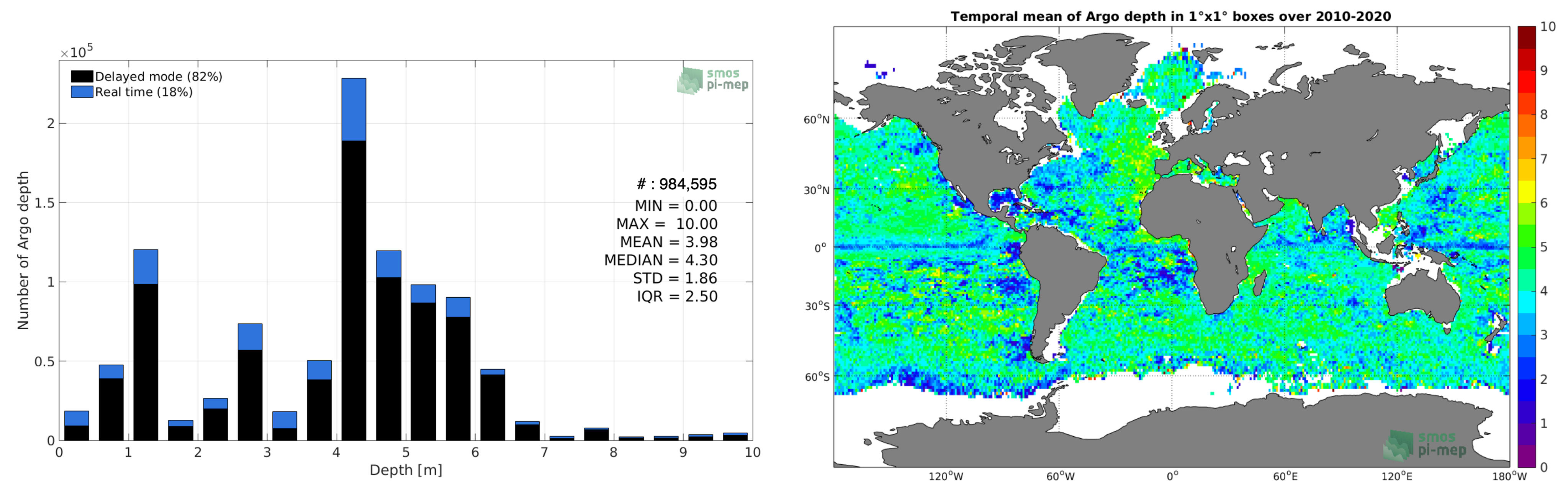
3.2.3. Distribution of In Situ SSS Depth Measurements
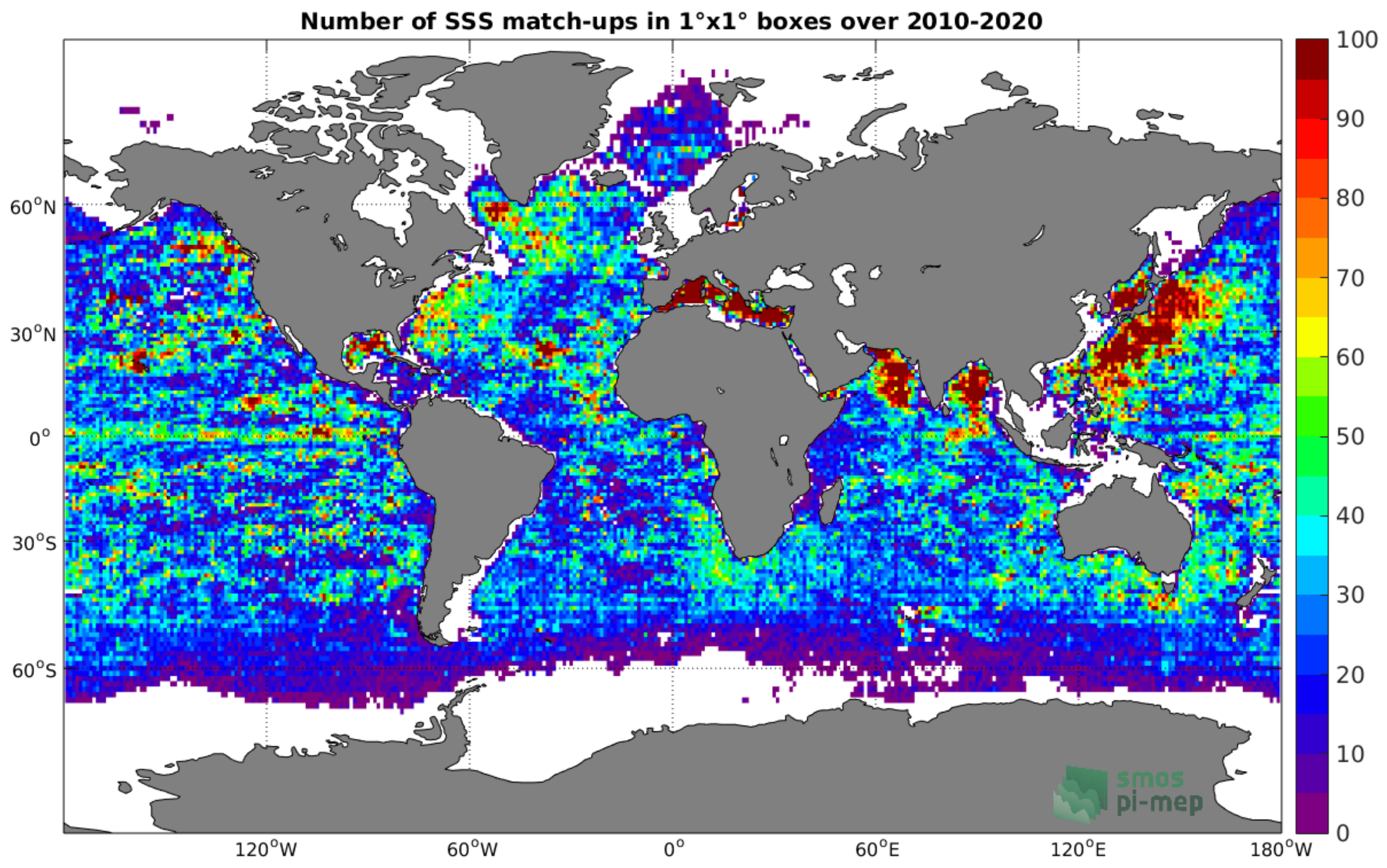
3.2.4. Spatial Distribution of Match-Ups
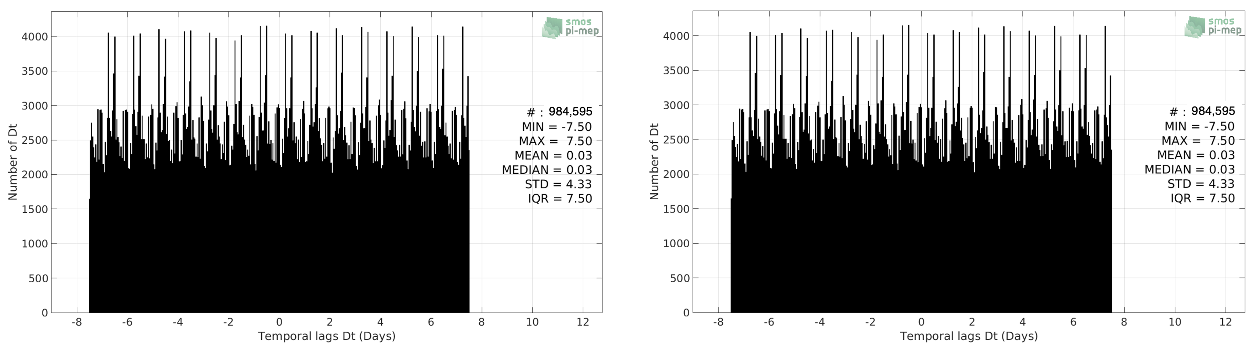
3.2.5. Histograms of the Spatial and Temporal Lags of the Match-Ups Pairs
3.3. Match-Up Analysis Report
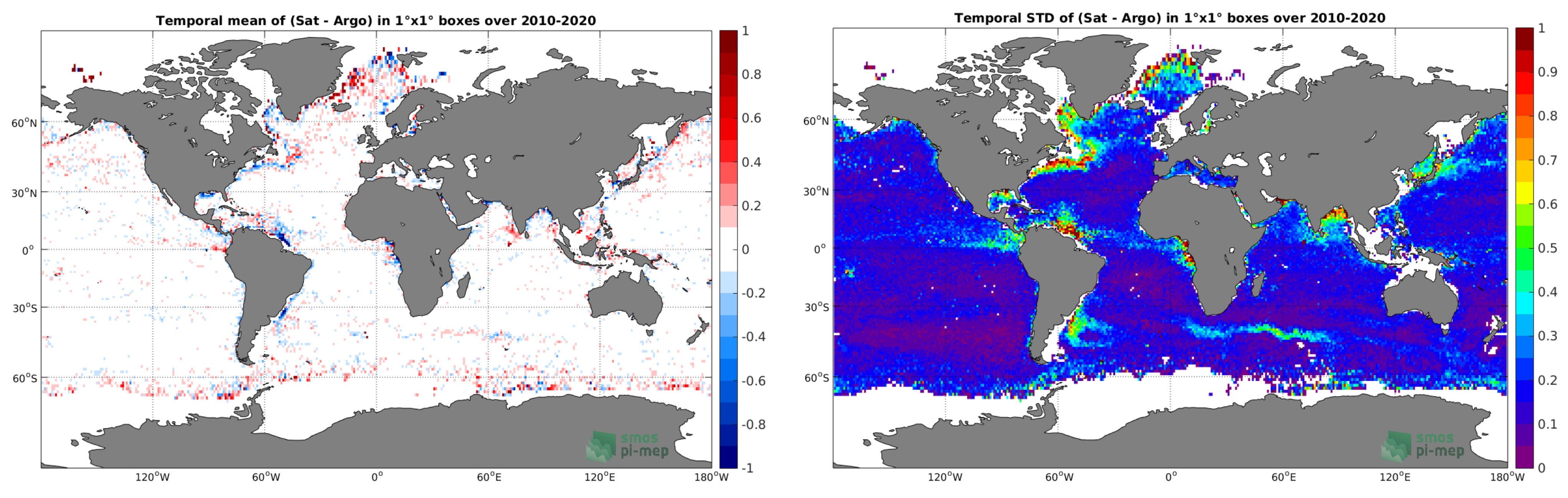
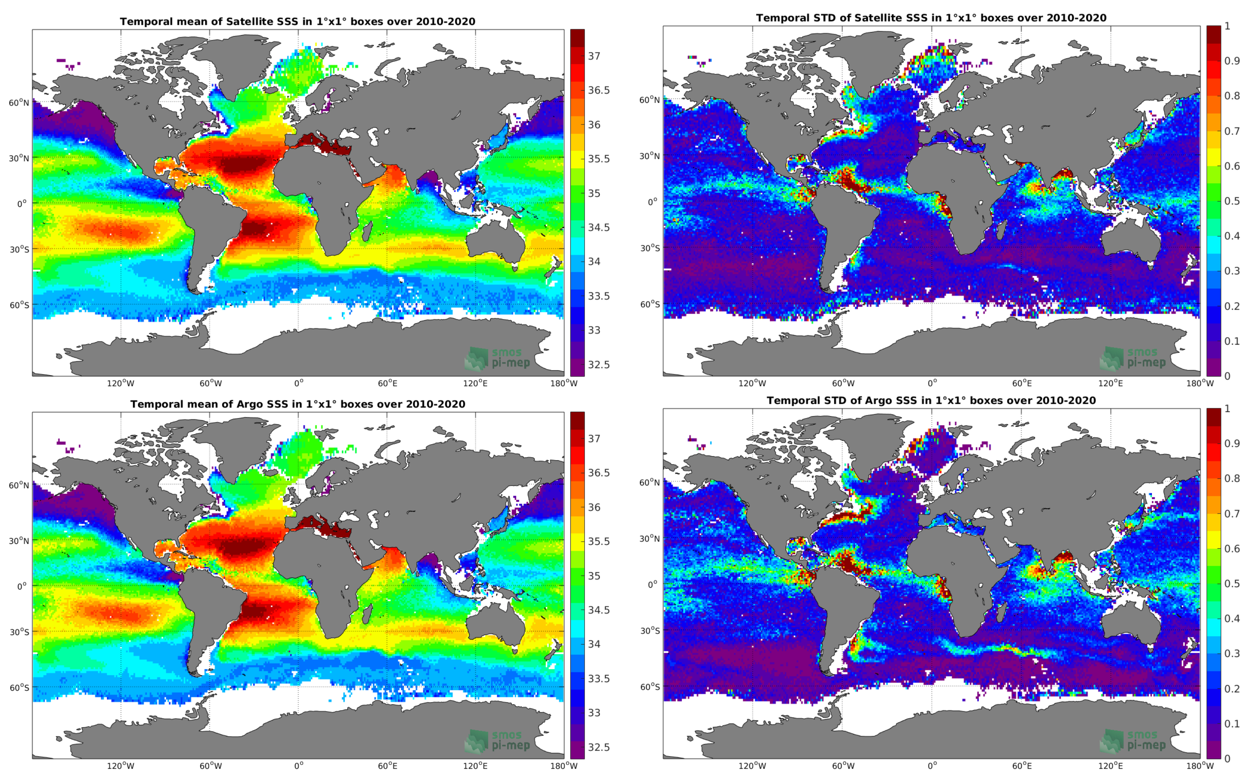
3.3.1. Spatial Maps of the Temporal Mean and STD of In Situ and Satellite SSS and of Their Difference (SSS)
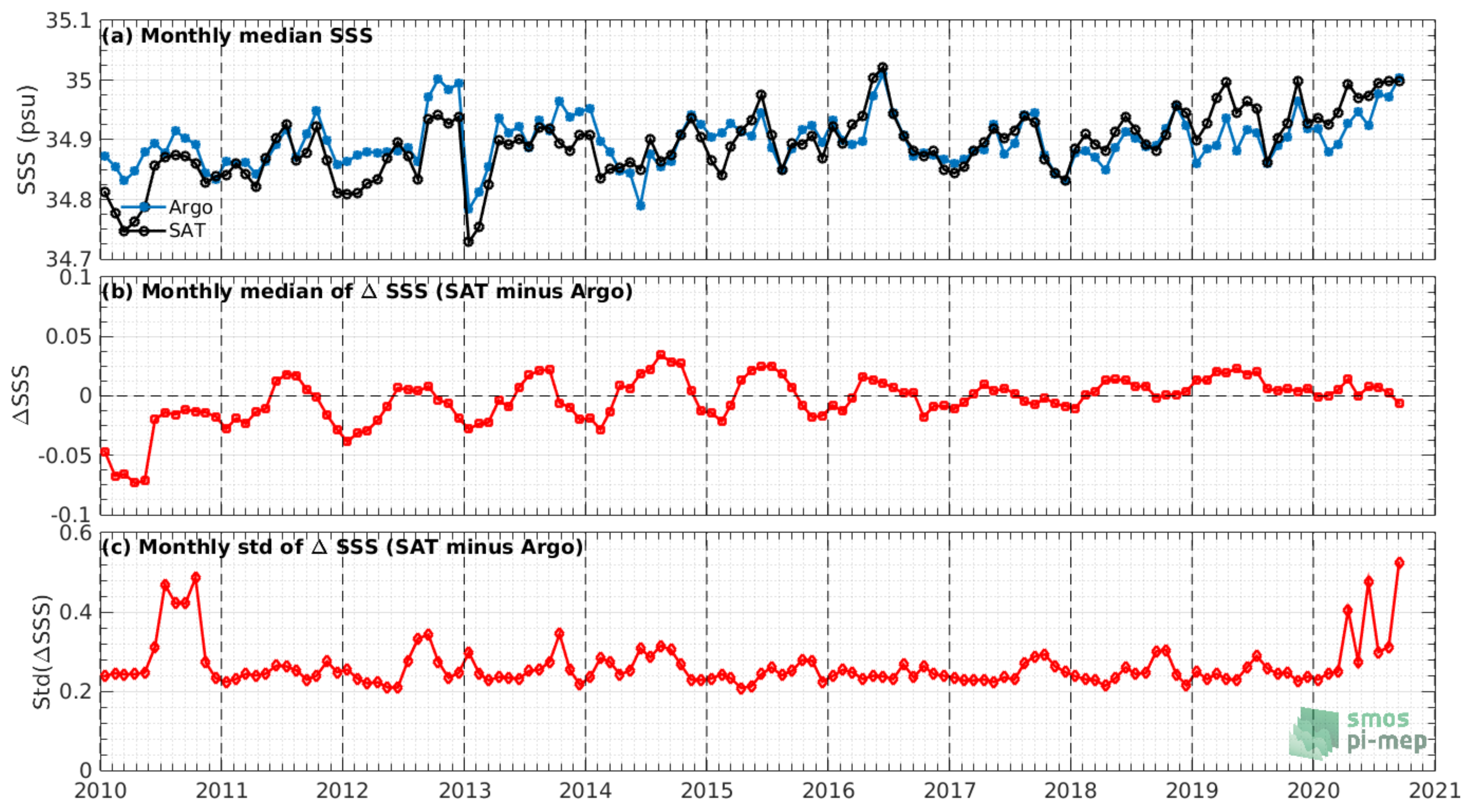
3.3.2. Time Series of the Monthly Median and STD of In Situ and Satellite SSS and of Their Difference (SSS)
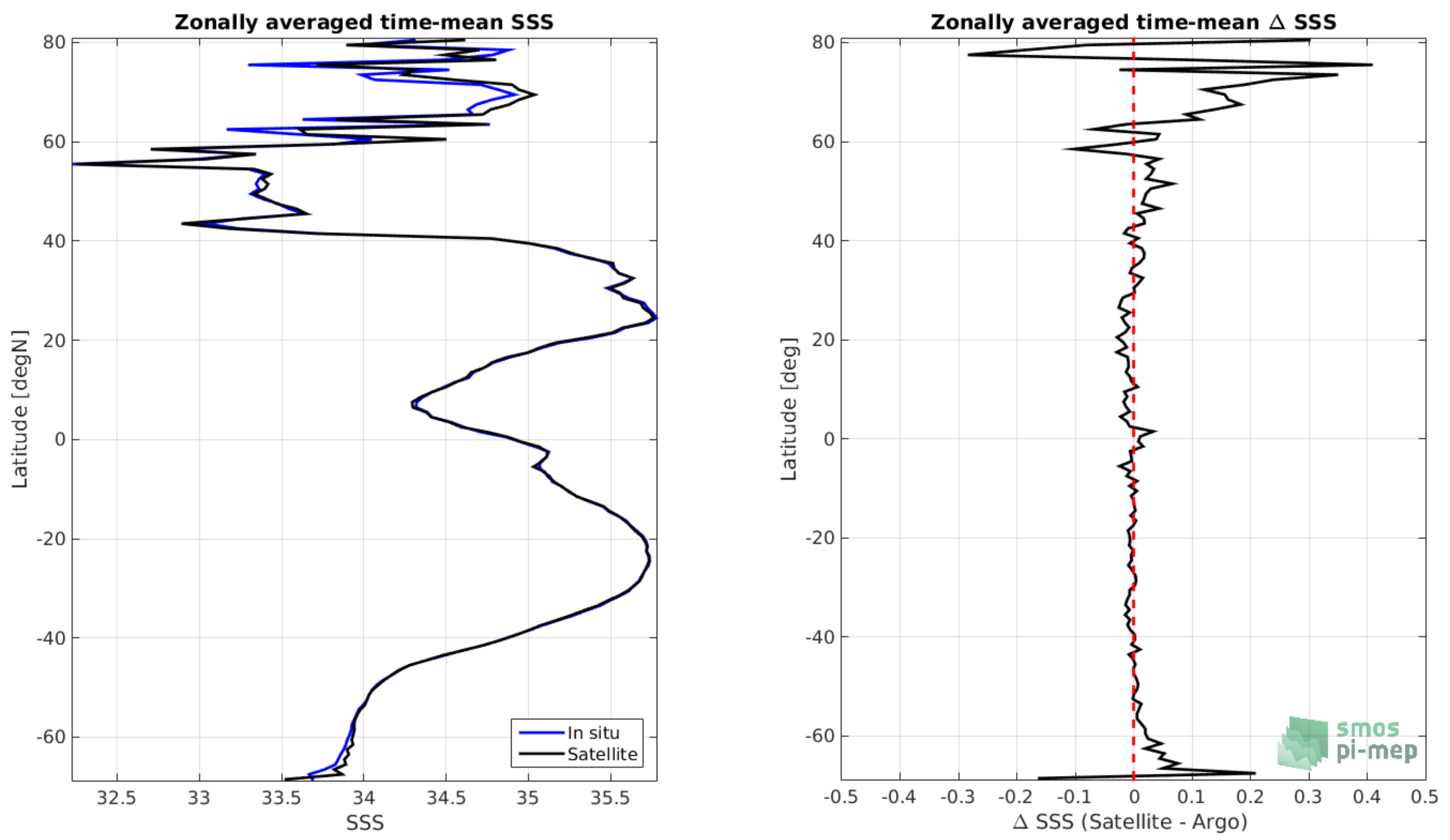
3.3.3. Zonal Mean and STD of In Situ and Satellite SSS and of Their Difference (SSS)
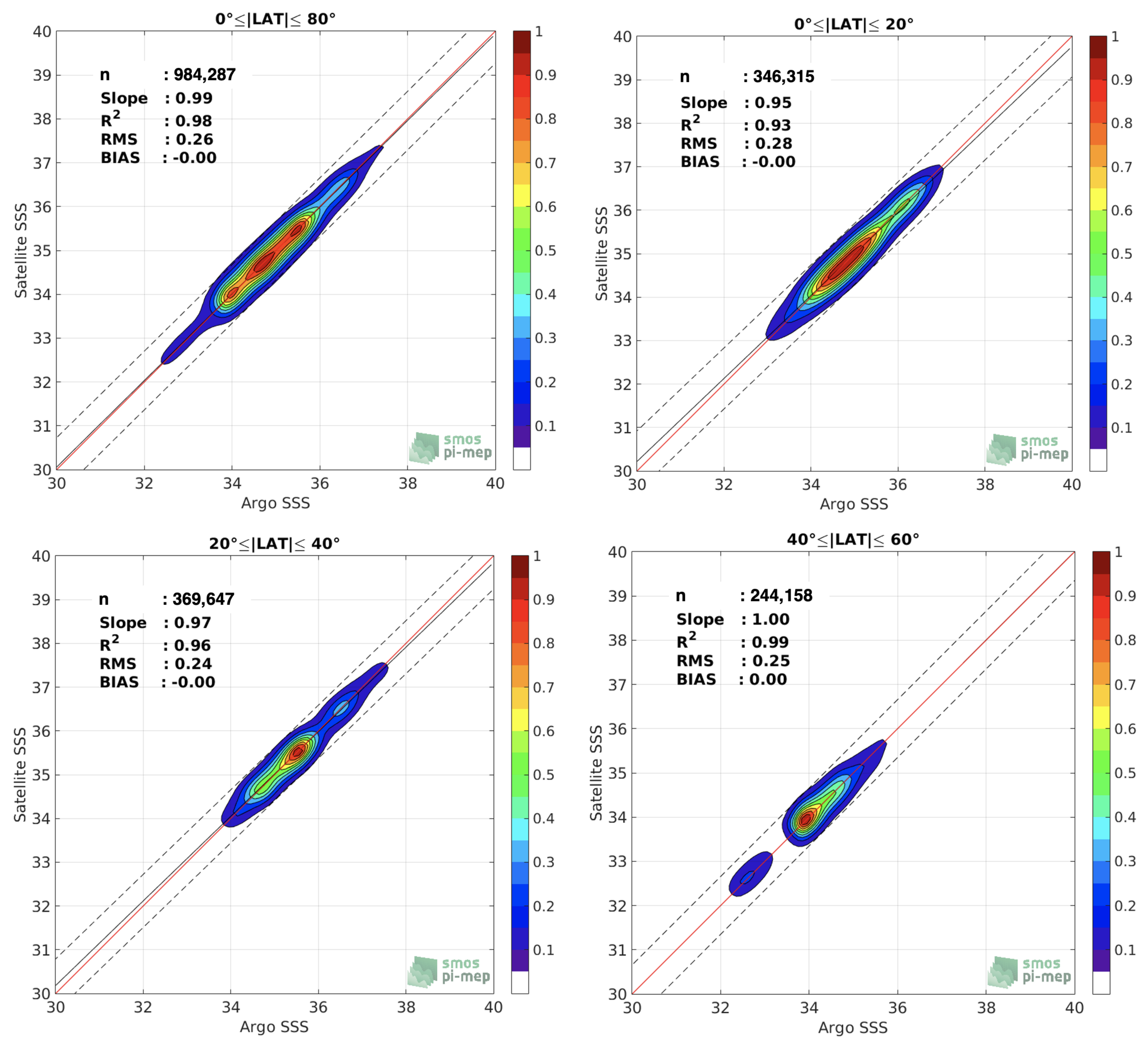
3.3.4. Scatterplots of Satellite versus In Situ SSS by Latitudinal Bands
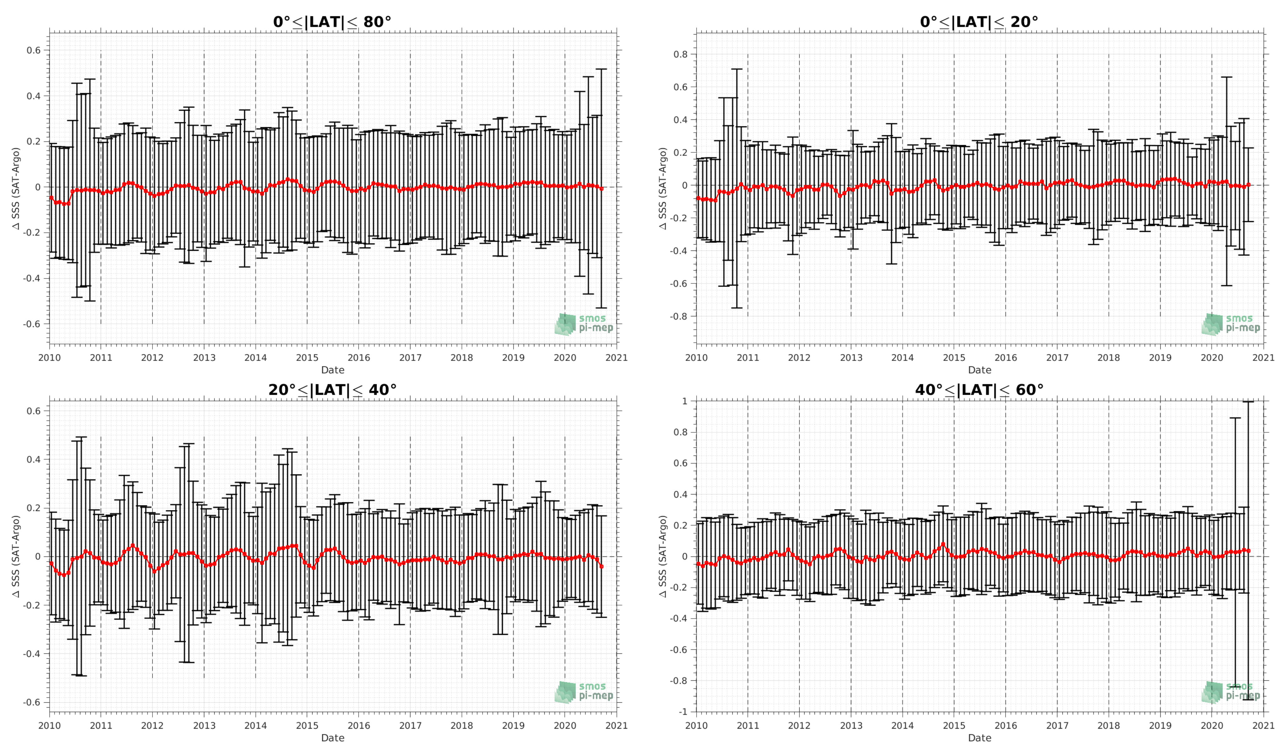
3.3.5. Time Series of the Monthly Median and STD of SSS Sorted by Latitudinal Bands
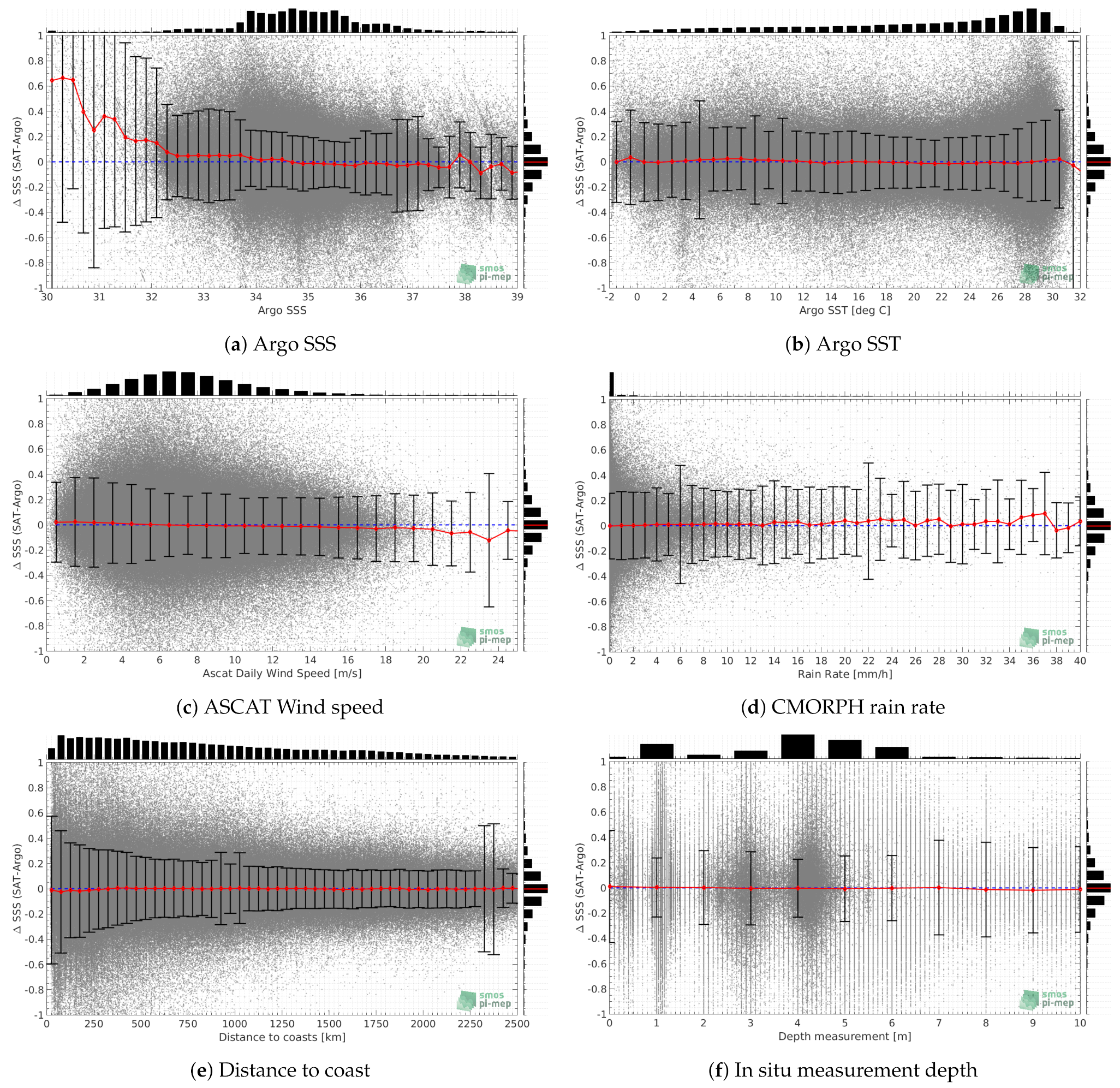
3.3.6. SSS Sorted as a Function of Geophysical Parameters
- In situ SSS values per bins of width 0.2;
- In situ SST values per bins of width 1 C;
- ASCAT daily wind values per bins of width 1 m/s;
- CMORPH 3-hourly rain rates per bins of width 1 mm/h;
- Distance to coasts per bins of width 50 km;
- In situ measurement depth (if relevant).
4. Exploitation: Tools and Case Studies
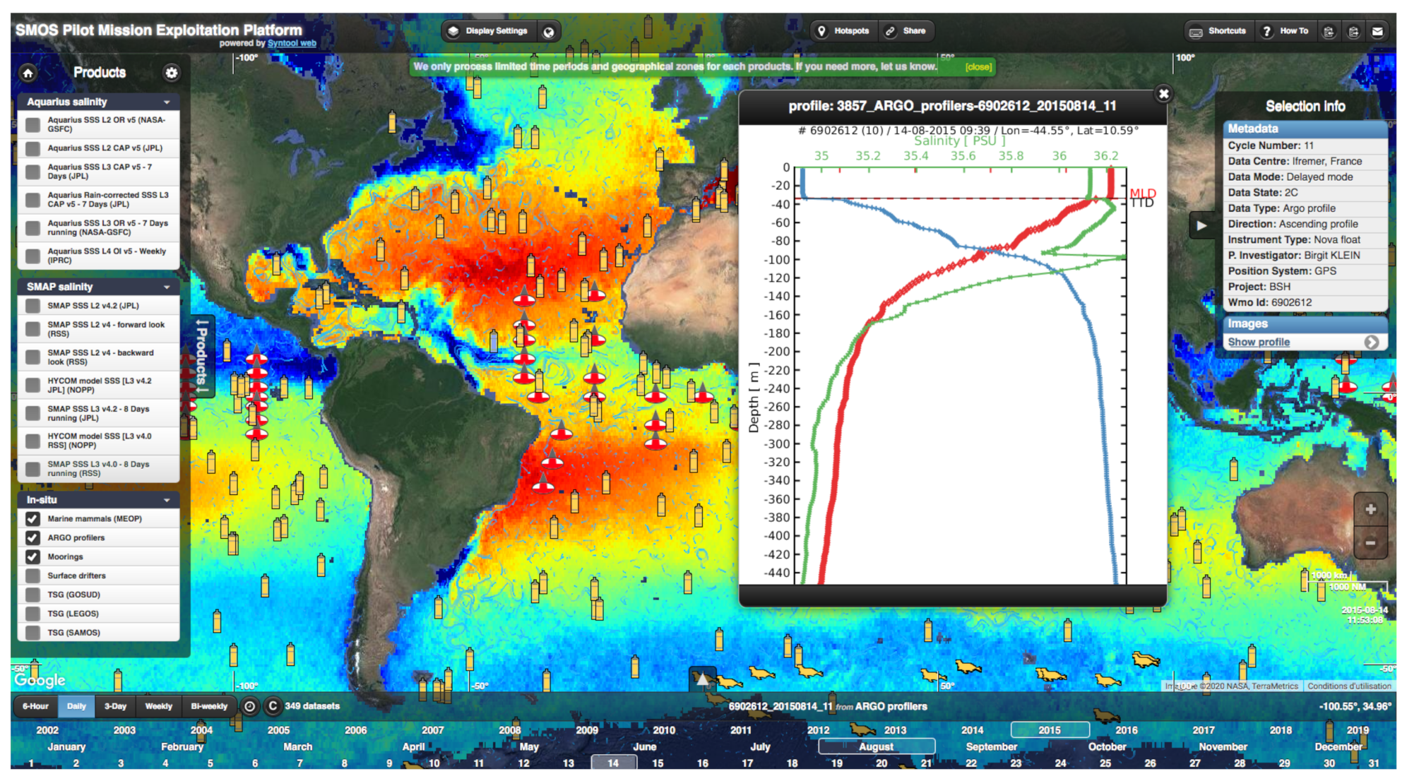
4.1. Syntool
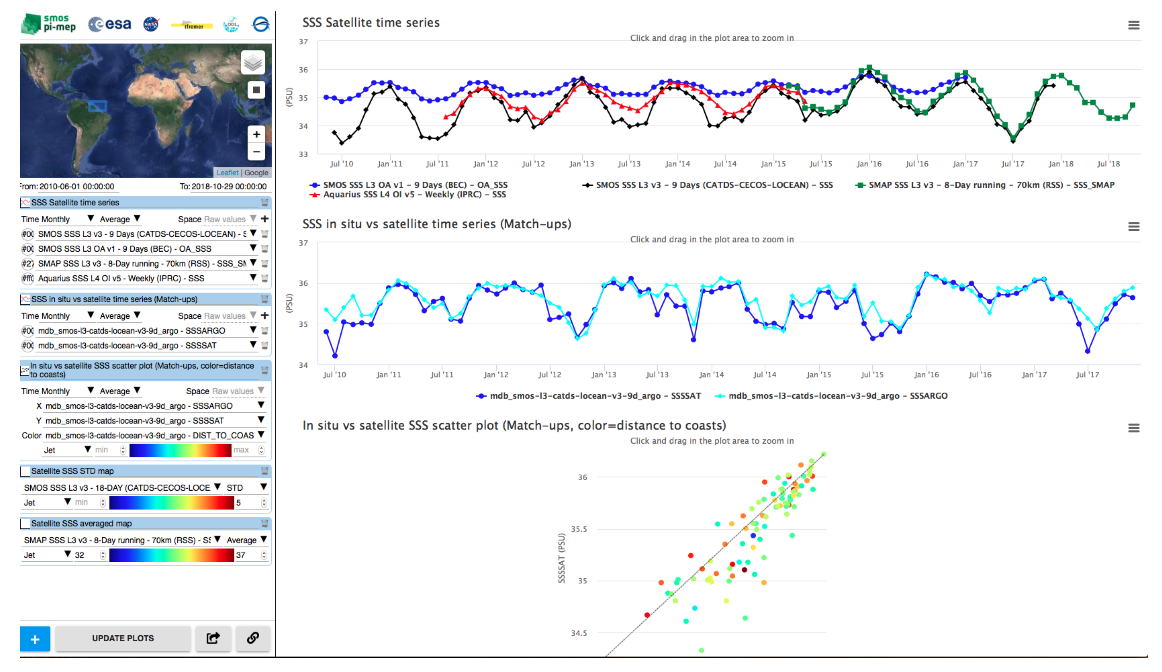
4.2. Plot Interface
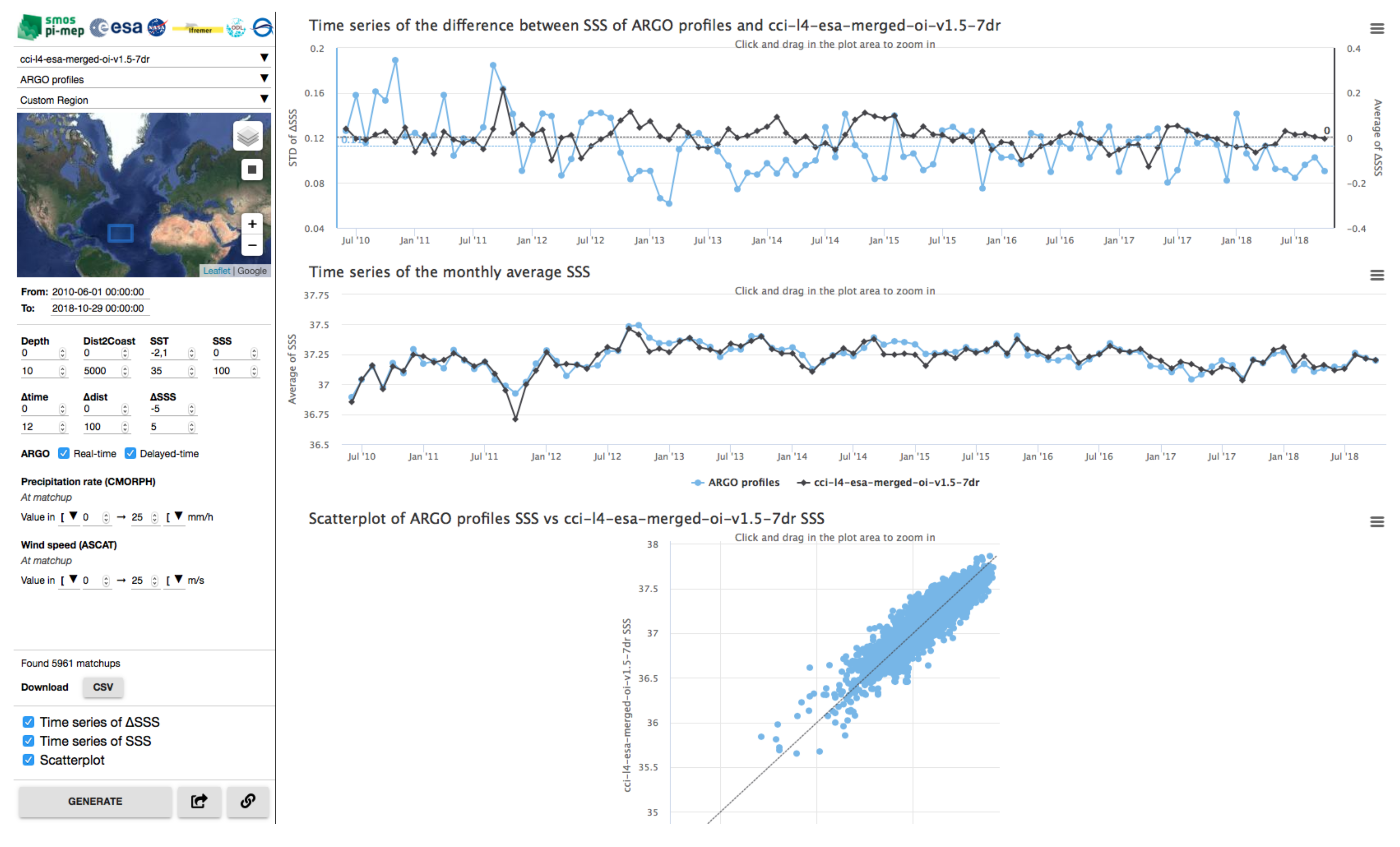
4.3. Match-Up Interface
- Depth of in situ measurements (between 0 and 10 m);
- Distance to coast (from 0 to 5000 km);
- SST range of the extraction in situ (from −2.1 to 35 C);
- SSS range of the extraction in situ (from 0 to 45);
- Temporal lag in the collocation process between the in situ date and SSS satellite data (between −16 and 16 days);
- Spatial lag in the collocation process between the in situ date and SSS satellite data (between 0 and 100 km);
- Real-time or delay mode or both (for Argo only);
- CMORPH rain rate at the time and location of the in situ measurement: filter if it is superior or inferior to a specified threshold (from 0 to 100 mm/h);
- ASCAT wind speed at the time and location of the in situ measurement: filter if it is superior/inferior to a specified threshold (from 0 to 30 m/s);
- Difference between in situ and satellite SSS values range (−5 to 5).
4.4. Merginator
4.5. Jupyter Notebooks
4.6. Case Studies
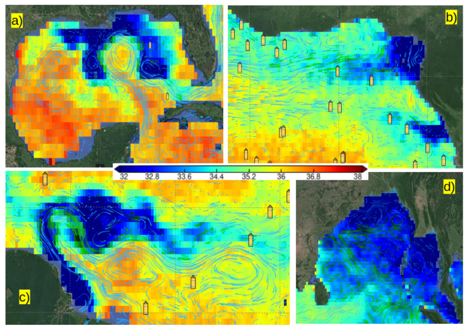
4.6.1. Case Study 1: Monitoring of Large River Plumes
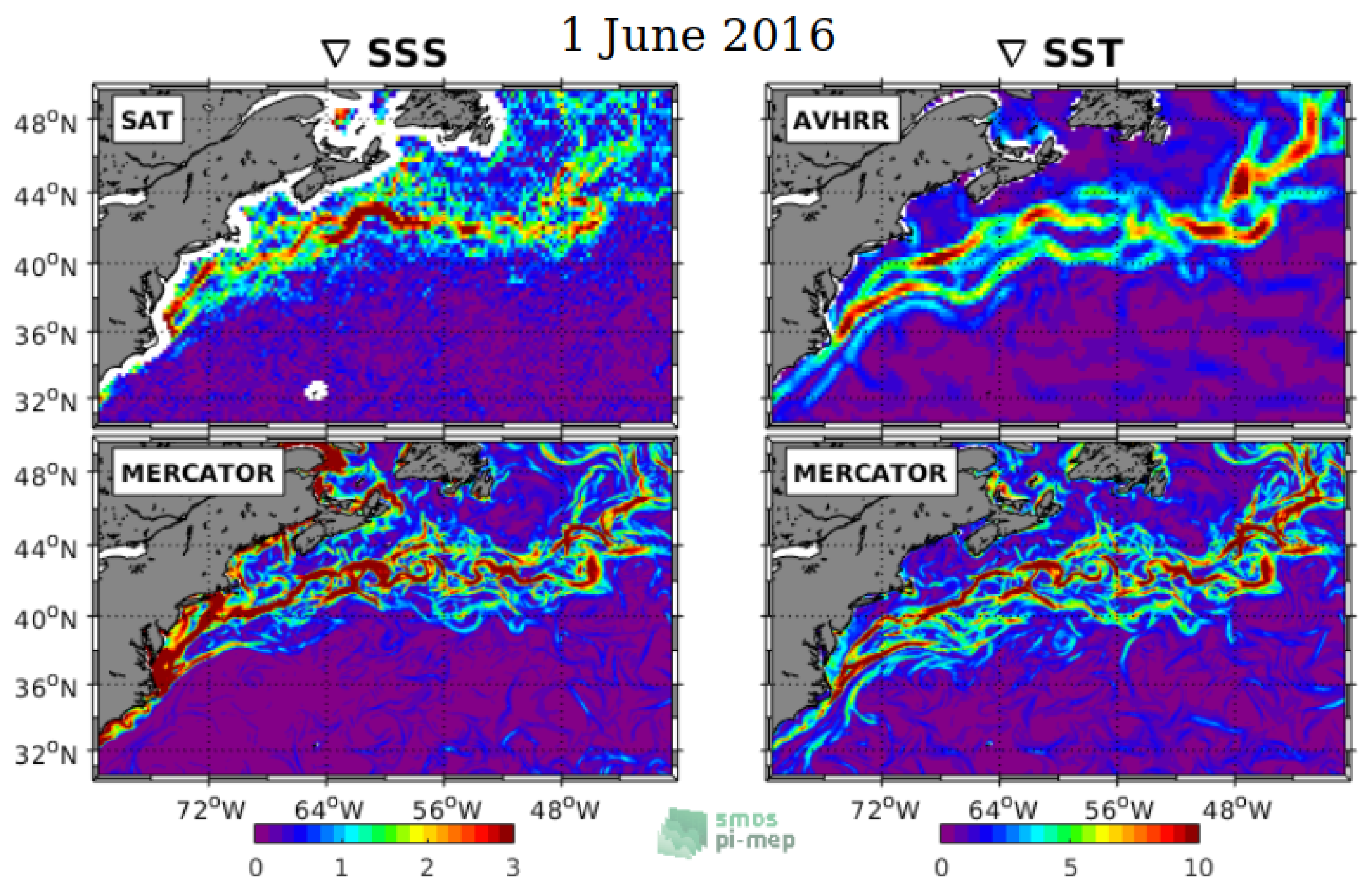
4.6.2. Case Study 2: Mesoscale Signatures in Western Boundary Currents
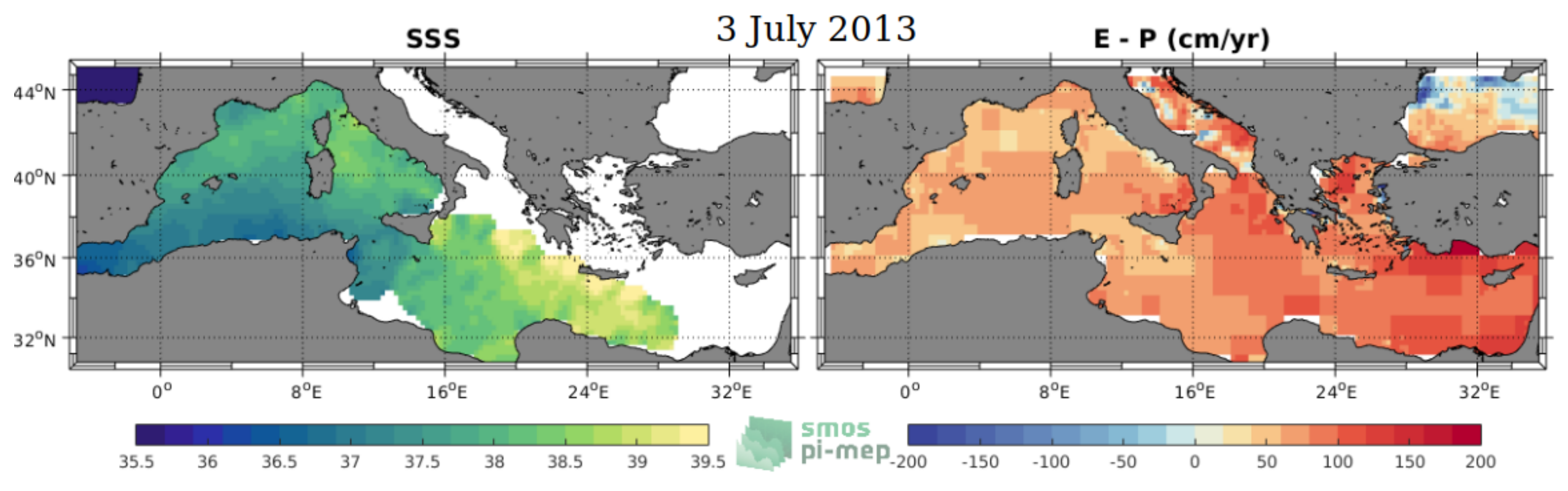
4.6.3. Case Study 3: High-Latitude and Semi-Enclosed Seas
4.6.4. Case Study 4: Salinity Processes in the Upper-Ocean Regional Studies (SPURS-2) Field Experiment
5. Summary and Conclusions
- Choose which satellite SSS product is best adapted for their own specific application;
- Improve the Level 2 to Level 4 SSS retrieval algorithms by better systematically identifying the conditions for which a given satellite SSS product is of good or degraded quality;
- Eventually converge towards the best validation and retrieval algorithm approaches and generate fewer satellite SSS products but with increased quality.
Author Contributions
Funding
Institutional Review Board Statement
Informed Consent Statement
Data Availability Statement
Acknowledgments
Conflicts of Interest
Abbreviations
| Aquarius | NASA/CONAE Salinity mission |
| ASCAT | Advanced Scatterometer |
| BLT | Barrier Layer Thickness |
| CCI | Climate Change Initiative |
| CMORPH | CPC MORPHing technique (precipitation analyses) |
| CPC | Climate Prediction Center |
| CTD | Instrument used to measure the conductivity, temperature, and pressure of seawater |
| DM | Delayed Mode |
| EO | Earth Observation |
| ESA | European Space Agency |
| FTP | File Transfer Protocol |
| GOSUD | Global Ocean Surface Underway Data |
| GTMBA | The Global Tropical Moored Buoy Array |
| Ifremer | Institut français de recherche pour l’exploitation de la mer |
| IPEV | Institut polaire français Paul-Émile Victor |
| ISAS | In Situ Analysis System |
| L2 | Level 2 |
| LEGOS | Laboratoire d’Etudes en Géophysique et Océanographie Spatiales |
| LOCEAN | Laboratoire d’Océanographie et du Climat: Expérimentations et |
| Approches Numériques | |
| LOPS | Laboratoire d’Océanographie Physique et Spatiale |
| MDB | Match-up Data Base |
| MEOP | Marine Mammals Exploring the Oceans Pole to Pole |
| MLD | Mixed Layer Depth |
| NCEI | National Centers for Environmental Information |
| NRT | Near Real Time |
| NTAS | Northwest Tropical Atlantic Station |
| OI | Optimal interpolation |
| Pi-MEP | Pilot-Mission Exploitation Platform |
| PIRATA | Prediction and Researched Moored Array in the Atlantic |
| QC | Quality control |
| Spatial resolution of the satellite SSS product | |
| RAMA | Research Moored Array for African-Asian-Australian Monsoon Analysis and |
| Prediction | |
| R | Square of the Pearson correlation coefficient: |
| RMS | Root mean square: |
| RR | Rain rate |
| SAMOS | Shipboard Automated Meteorological and Oceanographic System |
| Slope | Slope of a fitted line assuming an ordinary least squares regression model. |
| SMAP | Soil Moisture Active Passive (NASA mission) |
| SMOS | Soil Moisture and Ocean Salinity (ESA mission) |
| SPURS | Salinity Processes in the Upper Ocean Regional Study |
| SSS | Sea Surface Salinity |
| SSS | In situ SSS data considered for the match-up |
| SSS | Satellite SSS product considered for the match-up |
| SSS | Difference between satellite and in situ SSS at colocalized point |
| (SSS = SSS- SSS) | |
| SST | Sea Surface Temperature |
| STD | Standard deviation: |
| STD | Robust Standard deviation = median(abs(x-median (x)))/0.67 (less affected |
| by outliers than STD) | |
| Stratus | Surface buoy located in the eastern tropical Pacific |
| Survostral | SURVeillance de l’Océan AuSTRAL (Monitoring the Southern Ocean) |
| TAO | Tropical Atmosphere Ocean |
| TSG | ThermoSalinoGraph |
| WHOI | Woods Hole Oceanographic Institution |
| WHOTS | WHOI Hawaii Ocean Time-series Station |
| WOA | World Ocean Atlas |
References
- Reul, N.; Grodsky, S.A.; Arias, M.; Boutin, J.; Catany, R.; Chapron, B.; D’Amico, F.; Dinnat, E.; Donlon, C.; Fore, A.; et al. Salinity estimates from Spaceborne L-band radiometers: An overview of the first decade of observation (2010–2019). Remote Sens. Environ. 2020, 242, 111769. [Google Scholar] [CrossRef]
- Vinogradova, N.; Lee, T.; Boutin, J.; Drushka, K.; Fournier, S.; Sabia, R.; Stammer, D.; Bayler, E.; Reul, N.; Gordon, A.; et al. Satellite Salinity Observing System: Recent Discoveries and the Way Forward. Front. Mar. Sci. 2019, 6, 243. [Google Scholar] [CrossRef]
- Kilic, L.; Prigent, C.; Aires, F.; Boutin, J.; Heygster, G.; Tonboe, R.T.; Roquet, H.; Jimenez, C.; Donlon, C. Expected Performances of the Copernicus Imaging Microwave Radiometer (CIMR) for an All-Weather and High Spatial Resolution Estimation of Ocean and Sea Ice Parameters. J. Geophys. Res. 2018, 123, 7564–7580. [Google Scholar] [CrossRef] [Green Version]
- Pi-MEP. Match-up Datasets. 2021. Available online: https://www.salinity-pimep.org/data/mdb.html (accessed on 15 September 2021).
- Pi-MEP. Match-up Reports. 2021. Available online: https://www.salinity-pimep.org/reports/mdb.html (accessed on 15 September 2021).
- Pi-MEP. In-Situ Reports. 2021. Available online: https://www.salinity-pimep.org/reports/insitu.html (accessed on 15 September 2021).
- Gaillard, F.; Reynaud, T.; Thierry, V.; Kolodziejczyk, N.; von Schuckmann, K. In Situ-Based Reanalysis of the Global Ocean Temperature and Salinity with ISAS: Variability of the Heat Content and Steric Height. J. Clim. 2016, 29, 1305–1323. [Google Scholar] [CrossRef]
- Argo. Argo Float Data and Metadata from Global Data Assembly Centre (Argo GDAC). SEANOE 2021. [Google Scholar] [CrossRef]
- Alory, G.; Delcroix, T.; Téchiné, P.; Diverrès, D.; Varillon, D.; Cravatte, S.; Gouriou, Y.; Grelet, J.; Jacquin, S.; Kestenare, E.; et al. The French contribution to the voluntary observing ships network of sea surface salinity. Deep-Sea Res. Pt. I 2015, 105, 1–18. [Google Scholar] [CrossRef]
- Kolodziejczyk, N.; Diverres, D.; Jacquin, S.; Gouriou, Y.; Grelet, J.; Le Menn, M.; Tassel, J.; Reverdin, G.; Maes, C.; Gaillard, F. Sea Surface Salinity from French RESearcH Vessels: Delayed Mode Dataset, Annual Release. SEANOE 2020. [Google Scholar] [CrossRef]
- Reynaud, T.; Desprez De Gesincourt, F.; Gaillard, F.; Le Goff, H.; Reverdin, G. Sea Surface Salinity from Sailing Ships: Delayed Mode Dataset, Annual Release. SEANOE 2017. [Google Scholar] [CrossRef]
- Smith, S.R.; Rolph, J.J.; Briggs, K.; Bourassa, M.A. Quality-Controlled Underway Oceanographic and Meteorological Data from the Center for Ocean-Atmospheric Predictions Center (COAPS)—Shipboard Automated Meteorological and Oceanographic System (SAMOS). NOAA Natl. Cent. Environ. Inf. Dataset. 2009. [Google Scholar] [CrossRef]
- Morrow, R.; Kestenare, E. Nineteen-year changes in surface salinity in the Southern Ocean south of Australia. J. Mar. Sys. 2014, 129, 472–483. [Google Scholar] [CrossRef]
- Aulicino, G.; Cotroneo, Y.; Ansorge, I.; Van Den Berg, M. Sea Surface Temperature and Salinity Collected Aboard the S.A. AGULHAS II and S.A. AGULHAS in the South Atlantic Ocean and Southern Ocean from 2010-12-08 to 2017-02-02 (NCEI Accession 0170743). NOAA Natl. Cent. Environ. Inf. Dataset 2018. [Google Scholar] [CrossRef]
- Morisset, S.; Reverdin, G.; Boutin, J.; Martin, N.; Yin, X.; Gaillard, F.; Blouch, P.; Rolland, J.; Font, J.; Salvador, J. Surface salinity drifters for SMOS validation. Mercator Ocean—CORIOLIS Q. Newsl. 2012, 45, 33–37. [Google Scholar]
- Treasure, A.; Roquet, F.; Ansorge, I.; Bester, M.; Boehme, L.; Bornemann, H.; Charrassin, J.B.; Chevallier, D.; Costa, D.; Fedak, M.; et al. Marine Mammals Exploring the Oceans Pole to Pole: A Review of the MEOP Consortium. Oceanography 2017, 30, 132–138. [Google Scholar] [CrossRef]
- Roquet, F.; Guinet, C.; Charrassin, J.B.; Costa, D.P.; Kovacs, K.M.; Lydersen, C.; Bornemann, H.; Bester, M.N.; Muelbert, M.C.; Hindell, M.A.; et al. MEOP-CTD In-Situ Data Collection: A Southern Ocean Marine-Mammals Calibrated Sea Water Temperatures and Salinities Observations. SEANOE 2018. [Google Scholar] [CrossRef]
- Roemmich, D.; Gilson, J. The 2004–2008 mean and annual cycle of temperature, salinity, and steric height in the global ocean from the Argo Program. Prog. Oceanogr. 2009, 82, 81–100. [Google Scholar] [CrossRef]
- Boutin, J.; Chao, Y.; Asher, W.E.; Delcroix, T.; Drucker, R.; Drushka, K.; Kolodziejczyk, N.; Lee, T.; Reul, N.; Reverdin, G.; et al. Satellite and In Situ Salinity: Understanding Near-Surface Stratification and Sub-footprint Variability. Bull. Am. Meterol. Soc. 2016, 97, 1391–1407. [Google Scholar] [CrossRef] [Green Version]
- Joyce, R.J.; Janowiak, J.E.; Arkin, P.A.; Xie, P. CMORPH: A Method that Produces Global Precipitation Estimates from Passive Microwave and Infrared Data at High Spatial and Temporal Resolution. J. Hydrometeorol. 2004, 5, 487–503. [Google Scholar] [CrossRef]
- Bentamy, A.; Grodsky, S.A.; Carton, J.A.; Croizé-Fillon, D.; Chapron, B. Matching ASCAT and QuikSCAT winds. J. Geophys. Res. 2012, 117. [Google Scholar] [CrossRef] [Green Version]
- Banzon, V.; Smith, T.M.; Steele, M.; Huang, B.; Zhang, H.M. Improved Estimation of Proxy Sea Surface Temperature in the Arctic. J. Atmos. Oceanic Technol. 2020, 37, 341–349. [Google Scholar] [CrossRef]
- Nardelli, B.B.; Droghei, R.; Santoleri, R. Multi-dimensional interpolation of SMOS sea surface salinity with surface temperature and in situ salinity data. Remote Sens. Environ. 2016, 180, 392–402. [Google Scholar] [CrossRef]
- Cummings, J.A. Operational multivariate ocean data assimilation. Q. J. R. Meteor. Soc. 2005, 131, 3583–3604. [Google Scholar] [CrossRef] [Green Version]
- Cummings, J.A.; Smedstad, O.M. Variational Data Assimilation for the Global Ocean. In Data Assimilation for Atmospheric, Oceanic and Hydrologic Applications; Park, S.K., Xu, L., Eds.; Springer: Berlin/Heidelberg, Germany, 2013; Volume II, pp. 303–343. [Google Scholar] [CrossRef]
- Fox, D.N.; Teague, W.J.; Barron, C.N.; Carnes, M.R.; Lee, C.M. The Modular Ocean Data Assimilation System (MODAS). J. Atmos. Ocean. Technol. 2002, 19, 240–252. [Google Scholar] [CrossRef]
- Wunsch, C.; Heimbach, P.; Ponte, R.; Fukumori, I. The Global General Circulation of the Ocean Estimated by the ECCO-Consortium. Oceanography 2009, 22, 88–103. [Google Scholar] [CrossRef]
- Wunsch, C.; Heimbach, P. Chapter 21—Dynamically and Kinematically Consistent Global Ocean Circulation and Ice State Estimates. In Ocean Circulation and Climate; Academic Press: Cambridge, MA, USA, 2013. [Google Scholar] [CrossRef] [Green Version]
- Marshall, J.; Adcroft, A.; Hill, C.; Perelman, L.; Heisey, C. A finite-volume, incompressible Navier Stokes model for studies of the ocean on parallel computers. J. Geophys. Res. 1997, 102, 5753–5766. [Google Scholar] [CrossRef] [Green Version]
- Amante, C.; Eakins, B.W. ETOPO1 1 Arc-Minute Global Relief Model: Procedures, Data Sources and Analysis. In NOAA Technical Memorandum NESDIS NGDC-24; National Geophysical Data Center, NOAA: Washington, DC, USA, 2009. [Google Scholar] [CrossRef]
- Chelton, D.B.; deSzoeke, R.A.; Schlax, M.G.; El Naggar, K.; Siwertz, N. Geographical Variability of the First Baroclinic Rossby Radius of Deformation. J. Phys. Oceanogr. 1998, 28, 433–460. [Google Scholar] [CrossRef]
- de Boyer Montégut, C.; Madec, G.; Fischer, A.S.; Lazar, A.; Ludicone, D. Mixed layer depth over the global ocean: An examination of profile data and a profile-based climatology. J. Geophys. Res. 2004, 109. [Google Scholar] [CrossRef]
- de Boyer Montégut, C.; Mignot, J.; Lazar, A.; Cravatte, S. Control of salinity on the mixed layer depth in the world ocean: 1. General description. J. Geophys. Res. 2007, 112. [Google Scholar] [CrossRef]
- Pi-MEP. Case Studies: Large River Plumes Monitoring. 2021. Available online: https://www.salinity-pimep.org/case-studies/river-plumes/ (accessed on 15 September 2021).
- Pi-MEP. Case Studies: Mesoscale Signatures in Western Boundary Currents. 2021. Available online: https://www.salinity-pimep.org/case-studies/gulf-stream/ (accessed on 15 September 2021).
- Pi-MEP. Case Studies: High-Latitudes and Semi-Closed Seas. 2021. Available online: https://www.salinity-pimep.org/case-studies/high-latitude-and-semi-closed-sea/ (accessed on 15 September 2021).
- Pi-MEP. Case Studies: Field Campaign. 2021. Available online: https://www.salinity-pimep.org/case-studies/field-campaign/ (accessed on 15 September 2021).
- Lindstrom, E.; Edson, J.; Schanze, J.; Shcherbina, A. SPURS-2: Salinity Processes in the Upper-Ocean Regional Study 2—The Eastern Equatorial Pacific Experiment. Oceanography 2019, 32, 15–19. [Google Scholar] [CrossRef]
- Boutin, J.; Martin, N.; Kolodziejczyk, N.; Reverdin, G. Interannual anomalies of SMOS sea surface salinity. Remote Sens. Environ. 2016, 180, 128–136. [Google Scholar] [CrossRef]
- Pi-MEP. Changelog. 2021. Available online: https://www.salinity-pimep.org/changelog.html (accessed on 15 September 2021).


| In Situ Datasets | # | Time | Time | S | S | S |
|---|---|---|---|---|---|---|
| Argo | 1,478,178 | 1 January 2010 | 30 April 2021 | 0.04 | 40.45 | 34.75 |
| TSG (LEGOS-DM) | 6,478,390 | 1 January 2010 | 1 November 2020 | 0.03 | 42.74 | 34.63 |
| TSG (GOSUD-Research-vessel) | 5,413,749 | 5 January 2010 | 6 December 2019 | 0.01 | 42.00 | 35.68 |
| TSG (GOSUD-Sailing-ship) | 1,472,098 | 8 January 2010 | 29 August 2017 | 0.01 | 42.00 | 33.68 |
| TSG (SAMOS) | 23,815,136 | 7 January 2010 | 30 April 2021 | 05.03 | 39.80 | 33.35 |
| Marine mammals | 199,580 | 1 January 2010 | 14 January 2018 | 04.06 | 36.67 | 33.95 |
| Surface drifters | 2,215,429 | 1 January 2010 | 22 September 2020 | 01.03 | 44.22 | 35.62 |
| TSG (LEGOS-Survostral) | 654,661 | 1 January 2010 | 2 March 2020 | 22.67 | 35.73 | 34.17 |
| TSG (LEGOS-Surv-Adel) | 38,903 | 9 January 2010 | 25 January 2012 | 28.14 | 34.37 | 34.04 |
| Moorings | 6,520,601 | 1 January 2010 | 31 May 2021 | 27.02 | 37.81 | 34.95 |
| TSG (NCEI-0170743) | 590,389 | 8 December 2010 | 2 February 2017 | 32.41 | 35.78 | 34.26 |
| TSG (Polarstern) | 504,269 | 1 January 2010 | 11 October 2020 | 20.30 | 37.75 | 34.08 |
| Salinity Snake (SPURS-2) | 3,428,541 | 20 August 2016 | 13 November 2017 | 24.04 | 34.34 | 33.12 |
| Saildrone (SPURS-2) | 9218 | 16 October 2017 | 17 November 2017 | 30.75 | 33.85 | 33.29 |
| Waveglider (SPURS-2) | 642,340 | 24 August 2016 | 10 November 2017 | 27.48 | 34.47 | 33.51 |
| Seaglider (SPURS-2) | 73,542 | 24 August 2016 | 7 November 2017 | 28.99 | 34.86 | 33.27 |
| Total | 53,535,024 | 1 January 2010 | 31 May 2021 | 0.01 | 44.22 | 34.15 |
| Dataset Name | Level | Spatial Resolution | Temporal Coverage | Version | Provider |
|---|---|---|---|---|---|
| Temporal Resolution | Update Frequency | ||||
| SMOS SSS L2 v700 (ESA) | L2 | 30–80 km | From 1 June 2010 to present | v700 | ESA |
| 50-minute half-orbit (granule duration) | Daily | ||||
| SMAP SSS L2 v4 (RSS) | L2 | ∼70 km (grid 0.250.25) | From 27 March 2015 to present | v4 | RSS |
| 98-minute orbit (granule duration) | Daily | ||||
| SMAP SSS L2 v5 (JPL) | L2 | ∼60 km (25 km swath grid) | From 27 March 2015 to present | v5 | JPL |
| 98-minute orbit (granule duration) | Daily | ||||
| Aquarius SSS L2 OR v5 (NASA-GSFC) | L2 | 96 km × 390 km | From 25 August 2011 to 7 June 2015 | v5 | NASA Aquarius project |
| 98-minute orbit (granule duration) | End of mission data | ||||
| Aquarius SSS L2 CAP v5 (JPL) | L2 | 96 km × 390 km | From 25 August 2011 to 4 June 2015 | v5 | JPL |
| 98-minute orbit (granule duration) | End of mission data | ||||
| SMOS SSS L3 v317—10 Days (CATDS-CPDC) | L3 | ∼50 km (grid 25 km × 25 km) | From 1 January 2010 to present | v317 | CATDS CPDC |
| 10 days | 10 days | ||||
| SMOS SSS L3 v317—Monthly (CATDS-CPDC) | L3 | 50 km (grid 25 km × 25 km) | From 1 January 2010 to present | v317 | CATDS CPDC |
| Monthly | Monthly | ||||
| SMOS SSS L3 v5—9 Days (CATDS-CEC-LOCEAN) | L3 | ∼50 km (grid 25 km × 25 km) | From 16 January 2010 to 19 November 2020 | v5 | CATDS CEC LOCEAN |
| 9 days (every 4 days) | Yearly | ||||
| SMOS SSS L3 v5—18 Days (CATDS-CEC-LOCEAN) | L3 | ∼50 km (grid 25 km × 25 km) | From 16 January 2010 to 19 November 2020 | v5 | CATDS CEC LOCEAN |
| 18 days (every 4 days) | Yearly | ||||
| SMOS SSS L3 v2—Daily (CATDS-CEC-IFREMER) | L3 | 0.5 | From 1 May 2010 to 31 December 2017 | v2 | CATDS CEC IFREMER |
| Daily | - | ||||
| SMOS SSS L3 v2—Monthly (CATDS-CEC-IFREMER) | L3 | 0.25 | From 1 May 2010 to 31 December 2017 | v2 | CATDS CEC IFREMER |
| Monthly | - | ||||
| SMOS SSS L3 v2—9 Days (BEC) | L3 | 0.25 | From 24 January 2011 to 31 December 2019 | v2 | BEC |
| 9 days | - | ||||
| SMAP SSS L3 v5.0—8-Day running (JPL) | L3 | ∼60 km (grid 0.250.25) | From 27 March 2015 to present | v5 | JPL |
| 8-day running | 8 days | ||||
| SMAP SSS L3 v5.0—Monthly (JPL) | L3 | ∼60 km (grid 0.250.25) | From 27 March 2015 to present | v5 | JPL |
| Monthly | Monthly | ||||
| SMAP SSS L3 v4—8-Day running (RSS) | L3 | ∼70 km (grid 0.250.25) | From 27 March 2015 to present | v4 | RSS |
| 8-day running | Daily | ||||
| SMAP SSS L3 v4—Monthly (RSS) | L3 | ∼70 km (grid 0.250.25) | From 27 March 2015 to present | v4 | RSS |
| Monthly | Monthly | ||||
| Aquarius SSS L3 CAP v5—7-Day running (JPL) | L3 | 1 | From 25 August 2011 to 4 June 2015 | v5 | JPL |
| 7-day running | End of mission data | ||||
| Aquarius SSS L3 CAP v5—Monthly (JPL) | L3 | 1 | From 25 August 2011 to 4 June 2015 | v5 | JPL |
| Monthly | End of mission data | ||||
| Aquarius SSS L3 OR v5—7-Day running (NASA-GSFC) | L3 | 1 | From 25 August 2011- to 7 June 2015 | v5 | NASA Aquarius project |
| 7-day running | End of mission data | ||||
| Aquarius SSS L3 OR v5—Monthly (NASA-GSFC) | L3 | 1 | From 25 August 2011 to 7 June 2015 | v5 | NASA Aquarius project |
| Monthly | End of mission data | ||||
| SMOS SSS L3 v3—Monthly (ICDC) | L3 | 0.5 | From 1 May 2010 to 31 December 2016 | v3 | ICDC |
| Monthly | - | ||||
| SMOS SSS L4 v2—Weekly (CATDS-CEC-IFREMER) | L4 | 0.5 | From 1 May 2010 to 28 February 2017 | v2 | CATDS CEC IFREMER |
| Weekly | - | ||||
| SMOS SSS L4 FUSION (BEC) | L4 | 0.05 | From 24 January 2011 to 31 December 2019 | v2 | BEC |
| Daily | - | ||||
| Aquarius SSS L4 OI v5—Weekly (IPRC) | L4 | 0.5 | From 1 September 2011 to 3 June 2015 | v5 | IPRC |
| Weekly | End of mission data | ||||
| Aquarius SSS L4 OI v5—Monthly (IPRC) | L4 | 0.5 | From 1 September 2011 to 3 June 2015 | v5 | IPRC |
| Monthly | End of mission data | ||||
| CCI SSS L4 Merged-OI v3.2—7-day running (ESA) | L4 | 0.25 | From 6 January 2010 to 30 September 2020 | v3.2 | ESA |
| 7-day running | Yearly | ||||
| CCI SSS L4 Merged-OI v3.2—30-day running (ESA) | L4 | 0.25 | From 6 January 2010 to 15 September 2020 | v3.2 | ESA |
| 30-day running | Yearly | ||||
| SMAP SSS L4 OI v1—7 Days (IPRC) | L4 | 0.25 | From 28 September 2011 to 12 March 2021 | v1 | IPRC |
| 7 days | Yearly | ||||
| SMAP SSS L4 OI v1—Monthly (IPRC) | L4 | 0.25 | From September 2011 to February 2021 | v1 | IPRC |
| Monthly | Yearly |
| Dataset Name | Level | Spatial Resolution | Temporal Coverage | Version | Provider |
|---|---|---|---|---|---|
| Temporal Resolution | Update Frequency | ||||
| SMOS SSS L3 Arctic v1.1—7-Day runing mean (CATDS-CEC-LOCEAN) | L3 | 25 km | From 1 June 2010 to 26 December 2019 | v1.1 | CATDS CEC LOCEAN |
| 7-day running mean | - | ||||
| SMOS SSS L3 Arctic v1.1—Monthly (CATDS-CEC-LOCEAN) | L3 | 25 km | From 1 June 2010 to 26 December 2019 | v1.1 | CATDS CEC LOCEAN |
| Monthly | - | ||||
| SMOS SSS L3 Arctic OA v2—9 Days (BEC) | L3 | 0.25 | From 1 January 2011 to 31 December 2017 2017 | v2 | BEC |
| 9 days | - | ||||
| SMOS SSS L3 Arctic v3.1—9 Days (BEC) | L3 | 25 km | From 1 January 2011 to 31 December 2019 | v3.1 | BEC |
| 9 days | - | ||||
| SMOS SSS L3 MED-ATL-OA v2—9 Days (BEC) | L3 | 0.25 | From 1 January 2011 to 31 December 2016 | v2 | BEC |
| 9 days | - | ||||
| SMOS SSS L4 MED-ATL-FUSION v2—Daily (BEC) | L4 | 0.05 | From 1 January 2011 to 31 December 2016 | v2 | BEC |
| 9 days | - | ||||
| Aquarius SSS L4 ATL-OI v5—Weekly (IPRC) | L4 | 0.25 | From 1 September 2011 to 3 June 2015 | v5 | IPRC |
| Weekly | End of mission data | ||||
| Aquarius SSS L4 ATL-OI v5—Monthly (IPRC) | L4 | 0.25 | From 1 September 2011 to 3 June 2015 | v5 | IPRC |
| Monthly | End of mission data |
Publisher’s Note: MDPI stays neutral with regard to jurisdictional claims in published maps and institutional affiliations. |
© 2021 by the authors. Licensee MDPI, Basel, Switzerland. This article is an open access article distributed under the terms and conditions of the Creative Commons Attribution (CC BY) license (https://creativecommons.org/licenses/by/4.0/).
Share and Cite
Guimbard, S.; Reul, N.; Sabia, R.; Herlédan, S.; Khoury Hanna, Z.E.; Piollé, J.-F.; Paul, F.; Lee, T.; Schanze, J.J.; Bingham, F.M.; et al. The Salinity Pilot-Mission Exploitation Platform (Pi-MEP): A Hub for Validation and Exploitation of Satellite Sea Surface Salinity Data. Remote Sens. 2021, 13, 4600. https://doi.org/10.3390/rs13224600
Guimbard S, Reul N, Sabia R, Herlédan S, Khoury Hanna ZE, Piollé J-F, Paul F, Lee T, Schanze JJ, Bingham FM, et al. The Salinity Pilot-Mission Exploitation Platform (Pi-MEP): A Hub for Validation and Exploitation of Satellite Sea Surface Salinity Data. Remote Sensing. 2021; 13(22):4600. https://doi.org/10.3390/rs13224600
Chicago/Turabian StyleGuimbard, Sébastien, Nicolas Reul, Roberto Sabia, Sylvain Herlédan, Ziad El Khoury Hanna, Jean-Francois Piollé, Frédéric Paul, Tong Lee, Julian J. Schanze, Frederick M. Bingham, and et al. 2021. "The Salinity Pilot-Mission Exploitation Platform (Pi-MEP): A Hub for Validation and Exploitation of Satellite Sea Surface Salinity Data" Remote Sensing 13, no. 22: 4600. https://doi.org/10.3390/rs13224600
APA StyleGuimbard, S., Reul, N., Sabia, R., Herlédan, S., Khoury Hanna, Z. E., Piollé, J.-F., Paul, F., Lee, T., Schanze, J. J., Bingham, F. M., Le Vine, D., Vinogradova-Shiffer, N., Mecklenburg, S., Scipal, K., & Laur, H. (2021). The Salinity Pilot-Mission Exploitation Platform (Pi-MEP): A Hub for Validation and Exploitation of Satellite Sea Surface Salinity Data. Remote Sensing, 13(22), 4600. https://doi.org/10.3390/rs13224600