Article

Crop Rotation Modeling for Deep Learning-Based Parcel Classification from Satellite Time Series

LASTIG Lab, Université Gustave Eiffel, IGN-ENSG, F-94160 Saint-Mandé, France
*
Author to whom correspondence should be addressed.
Remote Sens. 2021, 13(22), 4599; https://doi.org/10.3390/rs13224599
Submission received: 11 October 2021 / Revised: 28 October 2021 / Accepted: 10 November 2021 / Published: 16 November 2021

Abstract

:
While annual crop rotations play a crucial role for agricultural optimization, they have been largely ignored for automated crop type mapping. In this paper, we take advantage of the increasing quantity of annotated satellite data to propose to model simultaneously the inter- and intra-annual agricultural dynamics of yearly parcel classification with a deep learning approach. Along with simple training adjustments, our model provides an improvement of over 6.3% mIoU over the current state-of-the-art of crop classification, and a reduction of over 21% of the error rate. Furthermore, we release the first large-scale multi-year agricultural dataset with over 300,000 annotated parcels.

Graphical Abstract

1. Introduction

The Common Agricultural Policy (CAP) is responsible for the allocation of agricultural subsidies in the European Union, which nears EUR 50 billion each year [1]. As a consequence, monitoring the crop types of for subsidy allocation represents a major challenge for payment agencies, which have encouraged the development of automated crop classification tools based on machine learning [2]. In particular, The Sentinels for Common Agricultural Policy (Sen4CAP) project [3] aims to provide EU member states with algorithmic solutions and best practice studies on crop monitoring based on satellite data from the Sentinel constellation [4]. Despite the inherent difficulty of differentiating between the complex growth patterns of plants, this task is made possible by the near limitless access to data and annotations. Indeed, Sentinel-2 offers multi-spectral observations at a high revisit time of five days on average, which are particularly appropriate for characterizing the complex spectral and temporal characteristics of crop phenology. Moreover, farmers declare the crop cultivated in each of their parcels every year. This represents over 10 million of annotations each year for France alone [5], all open accessible in the Land-Parcel Identification System (LPIS). However, the sheer scale of the problem raises interesting computational challenges: Sentinel-2 gathers over 25Tb of data each year over Europe.
The state-of-the-art of yearly parcel-based crop type classification from Satellite Image Time Series (SITS) is particularly dynamic, especially since the adoption of deep learning methods [6,7,8]. However, most methods operate on a single year worth of temporal acquisitions and ignore inter-annual crop rotations. In this paper, we propose the first deep learning framework for classifying yearly crop types from information spanning several years, as represented in Figure 1. We show that with straightforward alterations of the top-performing models and their training protocols, we can improve their predictions by a large margin.

1.1. Single-Year Crop-Type Classification

Single-year crop-type classification involves the classification of the crop grown in a parcel from a single year worth of observation. Pre-deep learning parcel-based classification methods rely on such as support vector machines [9] or random forests [10] operating on handcrafted descriptors such as the Normalized Difference Vegetation Index. The temporal dynamics are typically handled with stacking [10], probabilistic graphical models [11], or dynamic warping method [12].
The adoption of deep learning-based methods, in conjunction with growing data availability, has allowed for a large increase in performance for parcel-based crop classification. The spatial dimension of parcels is typically handled with convolutional neural networks [13], parcel-based statistics [8], or set-based encoders [14]. The temporal dynamics are modeled with temporal convolutions [7], recurrent neural networks [14], hybrid convolutional-recurrent networks [15], and temporal attention [6,8,16].
Multiple recent studies [6,17,18,19,20] have solidified the PSE+LTAE (Pixel Set Encoder and Lightweight Temporal Attention) as the state-of-the-art of crop type classification. Furthermore, this network is particularly parsimonious in terms of computation and memory usage, which proves well suited for training on multi-year data. Finally, the code is freely available (https://github.com/VSainteuf/lightweight-temporal-attention-pytorch, accessed on 10 October 2021). For these reasons, we choose to use this network as the basis for our analysis and design modifications.

1.2. Multi-Year Agricultural Optimization

Most of the literature on multi-year crop rotation focuses on agricultural optimization, i.e., the improvement of agricultural practices aiming to improve yields. These models generate suggested rotations according to expert knowledge [21], handcrafted rules [22], or statistical analysis [23]. Other models are based on a physical analysis of the soil composition [24] such as the nitrogen cycle [25]. Aurbacher and Dabbert also take a simple economic model into account in their analysis [26]. More sophisticated models combine different sources of knowledge for better suggestions, such as ROTOR [27] or CropRota [28]. The RPG Explorer software [29] uses a second order Markov Chain for a more advanced statistical analysis of rotations.
Given the popularity of these tools, it is clear that the careful choice of cultivated crops can have a strong impact on agricultural yields and is the object of a meticulous attention from farmers. This is reinforced by the multi-model, multi-country meta-study of Kollas et al. [30], showing that multi-year modeling allows for a large increase in yield prediction. Consequently, we posit that a classification model with access to multi-year data will be able to learn inter-annual patterns to improve its accuracy.

1.3. Multi-Year Crop Type Classification

Multi-year crop type classification refer to the leveraging of information (satellite observations, past declarations) to improve the classification of the grown crop type in agricultural parcels. Osman et al. [31] propose to use probabilistic Markov models to predict the most probable crop type from the sequence of past cultivated crops of the previous 3 to 5 years. Giordano et al. [32] and Bailly et al. [33] propose to model the multi-year rotation with a second order chain-Conditional Random Field (CRF). Finally, Yaramasu et al. [34] were the first to propose to analyze multi-year data with a deep convolutional-recurrent model. However, they only chose one image per year, and hence do not model both inter- and intra-annual dynamics. In contrast, we propose to explicitly our model operates at both the intra-annual scale by using the sequence of yearly observation and the inter-annual scale by considering past declarations.
We list here the main contributions of this paper:
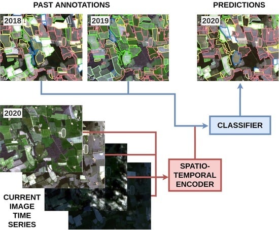
  • We propose a straightforward training scheme to leverage multi-year data and show its impact on yearly agricultural parcel classification.
  • We introduce a modified attention-based temporal encoder able to model both inter- and intra-annual dynamics of agricultural parcels, yielding a large improvement in terms of precision.
  • We present the first open-access multi-year dataset [35] for crop classification based on Sentinel-2 images, along with the full implementation of our model.
  • Our code in open-source at the following repository: https://github.com/felixquinton1/deep-crop-rotation, accessed on 11 November 2021.

2. Materials and Methods
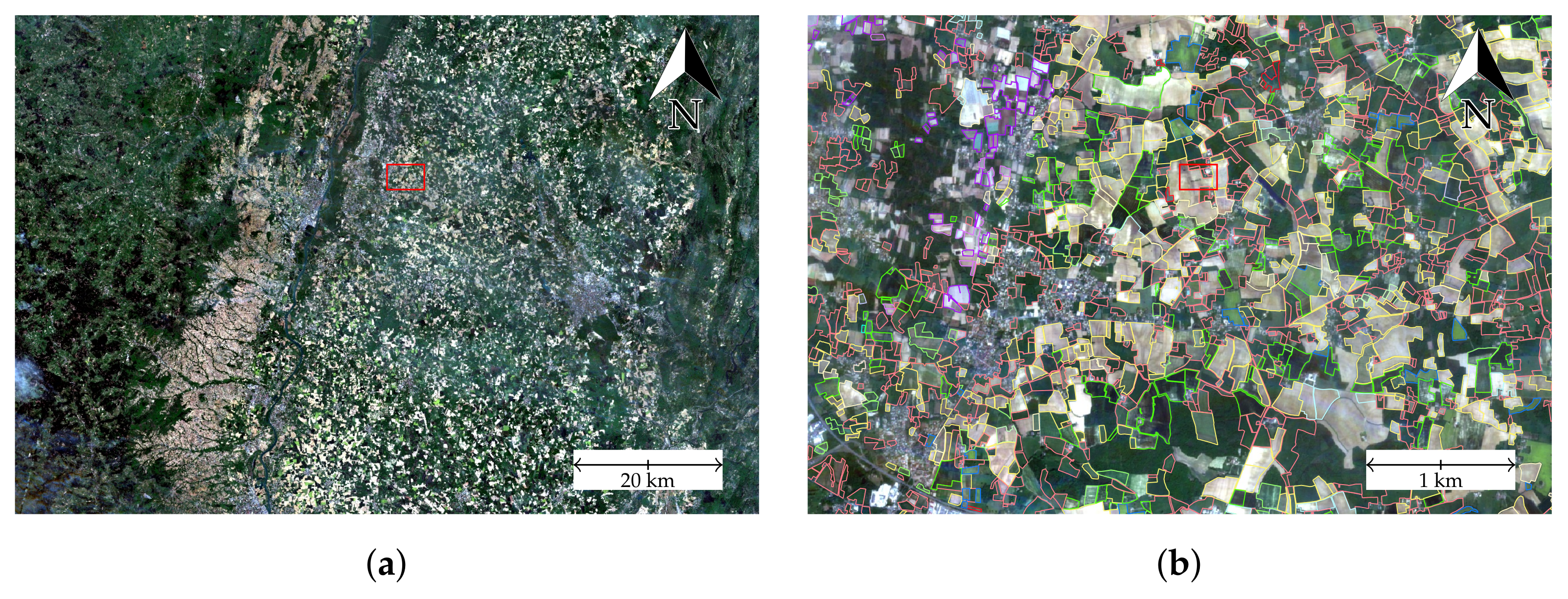
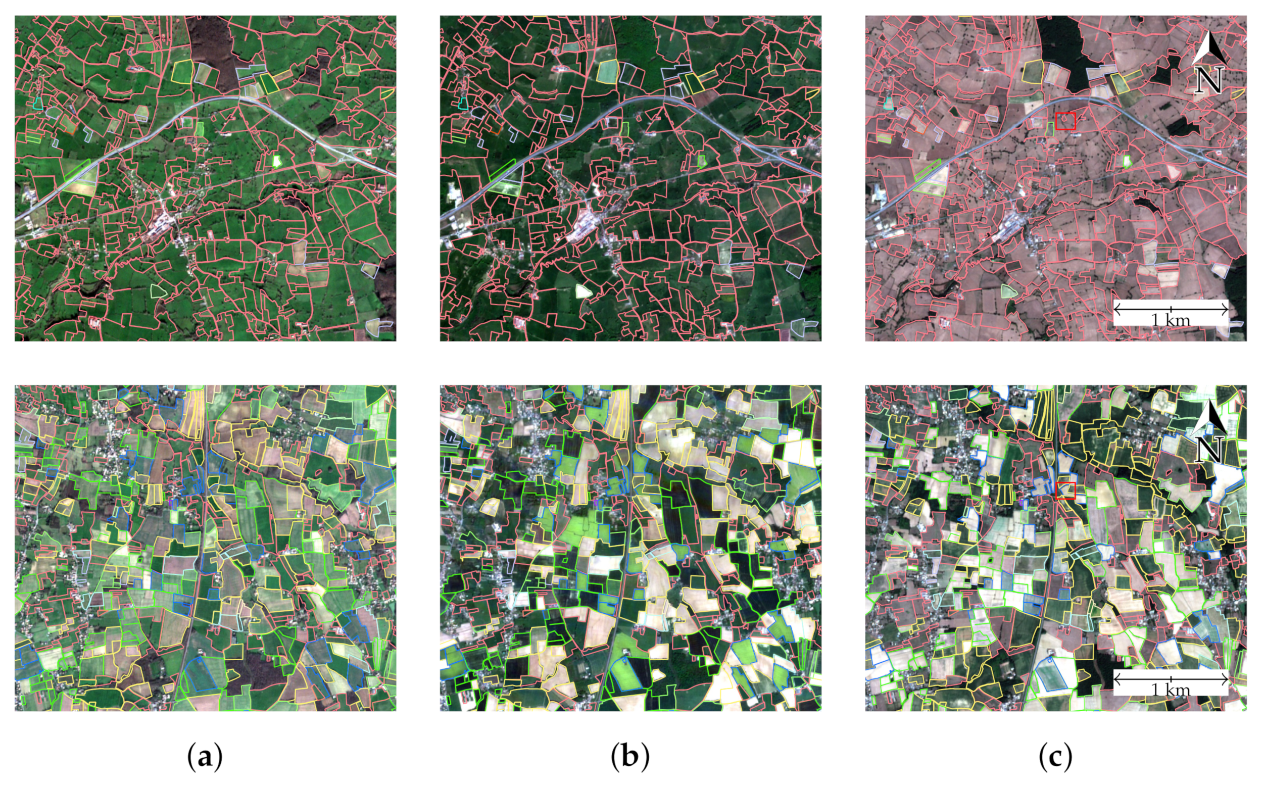
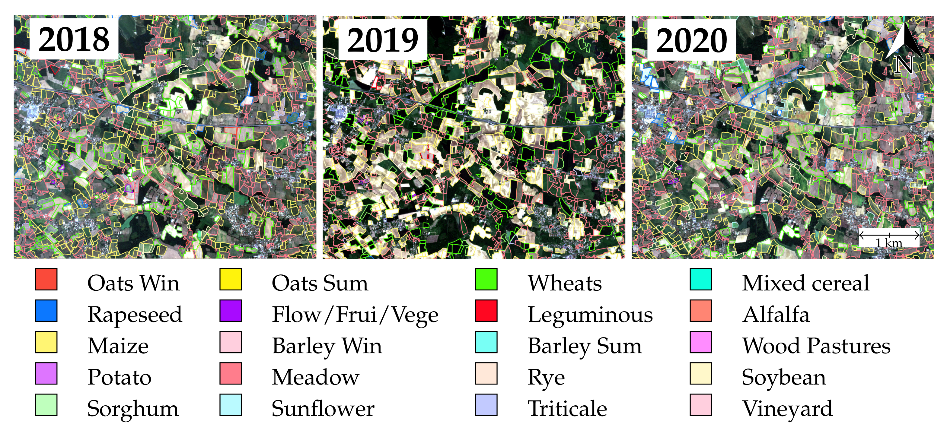
We present our dataset and proposed method to model multi-year SITS, along with several baseline methods to assess the performance of its components. We denote by [ 1 , I ] the set of years for which satellite observations are available to us, and use the compact pixel-set format to represent the SITS. For a given parcel and a year i [ 1 , I ] , we denote the corresponding SITS by a tensor x i of size C × S × T i , with C the number of spectral channels, S the number of pixels within the parcel, and T i the number of temporal observation available for year i. Likewise, we denote by l i { 0 , 1 } L the one-hot-encoded label at year i, denoting which kind of crop is cultivated in the considered parcel among a set L of crop types. Note that, in this article, we focus on the prediction of the main culture, i.e., only one crop type per year.

2.1. Dataset

Our proposed dataset, represented in Figure 2, is based on parcels within the 31TFM Sentinel-2 tile, covering an area of 110 × 110 km2 in the South East of France (centered around 4.31N, 46.44E in WGS84). This area, in the Auvergne-Rhône-Alpes region, is a major producer of cereal with over 54,000 ha of corn and 30,000 ha of wheat. Extensive livestock production makes meadow the most crop type with over 60% of declared parcels in the LPIS. The most frequent crop rotations are permanent cultures (meadows, vineyards, and pasture) and alternating between corn, wheat, and rapeseed.
Our satellite time series are constituted of Sentinel-2 level 2A images. We discard the bands B01, B09, and B10, and resample the remaining 10 spectral bands to a spatial resolution of 10 m per pixel with bilinear interpolation. Our data spans three years of acquisition: 2018, 2019, and 2020, with, respectively, 36, 27, and 29 valid entries, see Figure 3. The length of sequences varies due the automatic discarding of cloudy tiles by the data provider THEIA [36]. We do not apply further pre-processing such as cloud removal or radiometric calibration than what is already performed by the data provider THEIA.
We select stable parcels, meaning that their contours only undergo minor changes across the three studied years. We also discard very small parcels (under 800 m2) small or with very narrow shapes to reflect the resolution of the Sentinel-2 satellite. Each parcel has a ground truth cultivated crop type for each year corresponding to the main culture as reported by the French LPIS, whose precision is estimated at over 97% as reported by the French Payment Agency. Note that we ignore secondary cultures for parcels with multiple growth cycles. In order to limit class imbalance, we only keep crop types among a list of 20 of the most cultivated species in the area of interest. In sum, our dataset is composed of 103,602 parcels, each associated with three image time sequences and three crop annotations corresponding to the farmers’ declarations for 2018, 2019, and 2020.
The Sentinel2Agri dataset [6], composed of parcels from the same area, is composed of 191,703 parcels. We can estimate that our selection criteria exclude approximately every other parcel. A more detailed analysis of the evolving parcel partitions across different plots could lead to retaining a higher proportion of the original parcels.
As represented in Table 1, the dataset is still imbalanced: more than 60% of declarations correspond to meadows. In comparison, potato is cultivated in less than 100 parcels each year in the area of interest.

2.2. Pixel-Set and Temporal Attention Encoders

The Pixel Set Encoder (PSE) [6] is an efficient spatio-spectral encoder that learns expressive descriptors of the spectral distribution of the observations by randomly sampling pixels within a parcel. Its architecture is inspired by set-encoding deep architecture [13,37], and dispense us from preprocessing parcels into image patches, saving memory, and computation. The Temporal Attention Encoder (TAE) [6] and its parsimonious version Lightweight-TAE (LTAE) [18] are temporal sequence encoders based on the language processing literature [38] and adapted for processing SITS. Both networks can be used sequentially to map the sequence of observations x i at year i to a learned yearly spatio-temporal descriptor e i :
e i = TAE ( PSE ( x t i ) t = 1 T i ) .

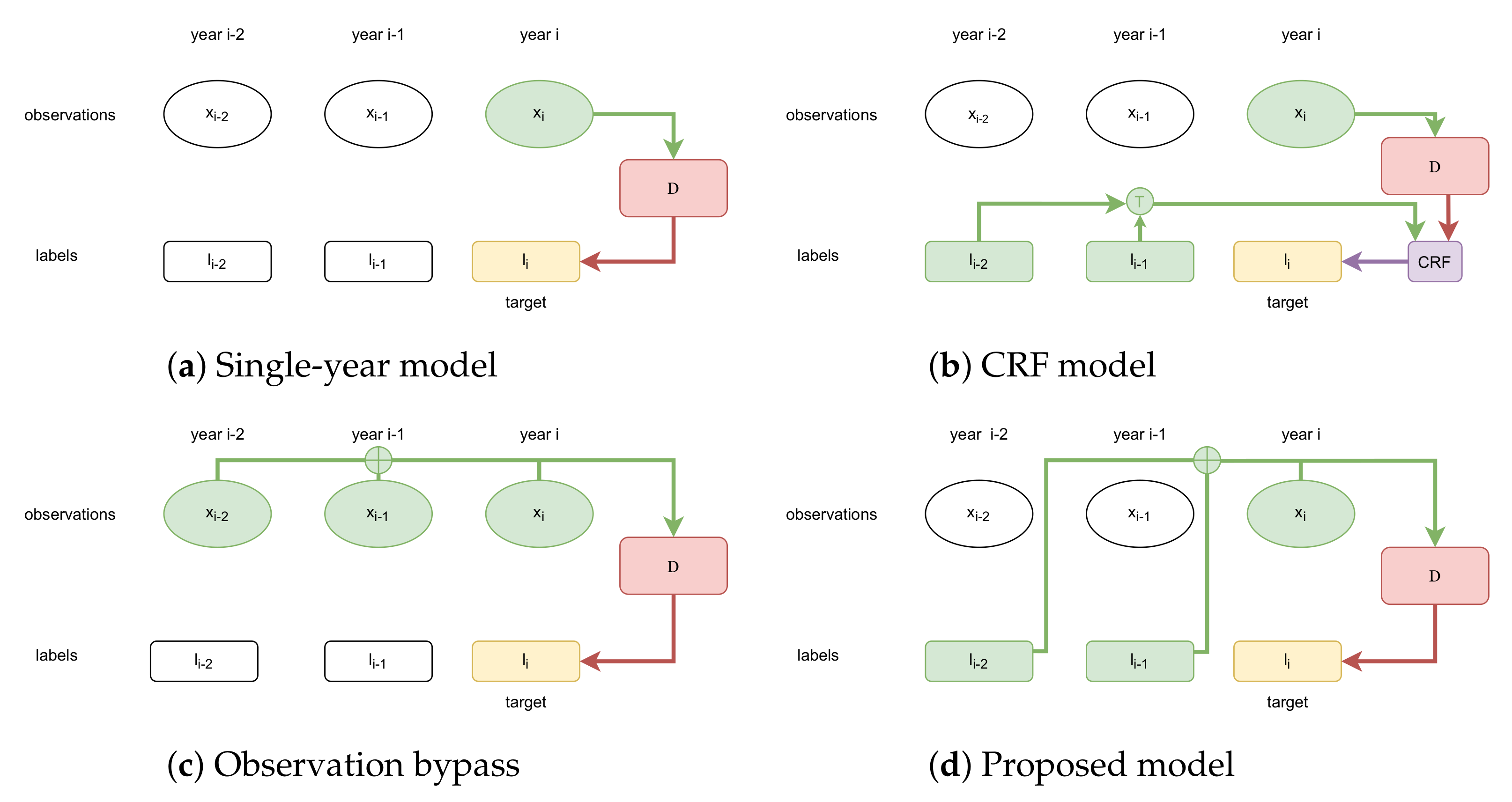
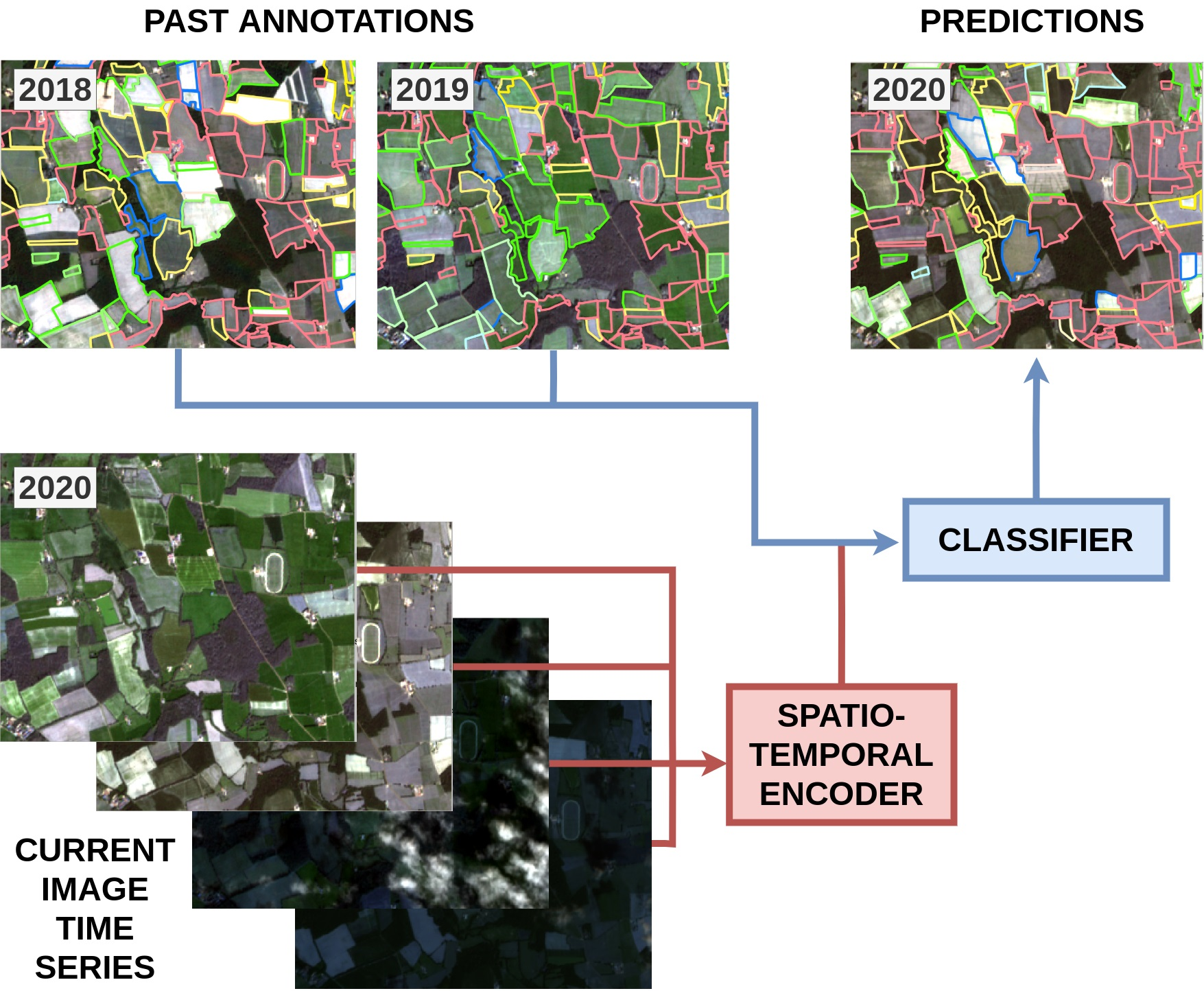
2.3. Multi-Year Modeling

We now present a simple modification of the PSE+LTAE network to model crop rotation. In the original PSE+LTAE approach, the descriptor e i is directly mapped to a vector of class scores z i by a Multi Layer Perceptron (MLP). In order to make the prediction z i covariant with past cultivated crops, we augment the spatio-temporal descriptors e i by concatenating the sum of the one-hot-encoded labels l j for the previous two years j = i 1 , i 2 . Then, a classifier network D , typically an MLP, maps this feature to a vector z i of L class scores:
z i = D e i | | l i 1 + l i 2 ,
with [ · | | · ] the channelwise concatenation operator. We handle the edge effects of the first two available years by defining l 0 and l 1 as vector of zero of size L (temporal zero-padding). This model can be trained end-to-end to simultaneously learn inter-annual crop rotations along with the intra-annual evolution of the parcels’ spectral statistics. Our model makes three simplifying assumptions:
  • We only consider the last two previous years because of the limited span of our available data. However, it would be straightforward to extend our approach to a longer duration.
  • We consider that the history of a parcel is completely described by its past cultivated crop types, and we do not take the past satellite observations into account. In other words, the label at year i is independent from past observations conditionally to its past labels [39] (Chapter 2). This design choice allows the model to stay tractable in terms of memory requirements.
  • The labels of the past two years are summed and not concatenated. The information about the order in which the crops were cultivated is then lost, but this results in a more compact model.

2.4. Baseline Models

In order to meaningfully evaluate the performance of our proposed approach, we implement different baselines for classifying parcels from multi-year data. In Figure 4, we represent schematically the main idea behind these baselines and our proposed approach. Note that the choice of backbone network to handle single-year data is out of the scope of this paper.
Single-Year:Msingle. We simply do not provide the labels of previous years, and directly map the current year’s observations to a vector of class scores [18].
Conditional Random Fields:MCRF. Based on the work of [32,33], we implement a simple chain-CRF probabilistic model. We use the prediction of the previous PSE+LTAE, calibrated with the method of Guo et al. [40] to approximate the posterior probability p [ 0 , 1 ] L of a parcel having the label k for year i: p k = P ( l i = k x i ) (see Section 3.3 for more details). We then model the second order transition probability p ( l i = k l i 1 , l i 2 ) with a three-dimensional tensor T [ 0 , 1 ] L × L × L that can be approximated based on the observed transitions in the training set. As suggested by Bailly et al., we use a Laplace regularization [41] (Chapter 13) to increase robustness. The resulting probability for a given year i is given by:
z CRF i [ k ] = p T [ l i 2 , l i 1 , : ] ,
with ⊙ the Hadamard term-wise multiplication. This method is restricted to i > 2 as edge effects are not straightforwardly fixed with padding.
Observation Bypass:Mobs. Instead of concatenating the labels of previous years to the embedding e i , we concatenate the average of the descriptors of the last two years e i 1 for e i 2 :
z obs i = D obs ( [ e i | | { 1 2 [ e i 1 + e i 2 ] if i > 1 e 0 if i = 1 0 if i = 0 ] ) .
Edge effects are handled with mirror and zero temporal-padding.
Label Concatenation:Mdec-concat. Instead of concatenating the sum of the last two previous years, we propose to concatenate each one-hot-encoded vector l i 1 and l i 2 with the learned descriptor z i . This approach is similar to Equation (2), but leads to a larger descriptor and a higher parameter count.
Single-Year Label Bypass:Mdec-one-year. In order to evaluate the impact of describing the history of parcels as the past two cultivated crops, we only concatenate the label of the previous year to the learned descriptor e i .

2.5. Training Protocol

We propose a simple training protocol to leverage the availability of observations and farmers’ declarations from multiple years.

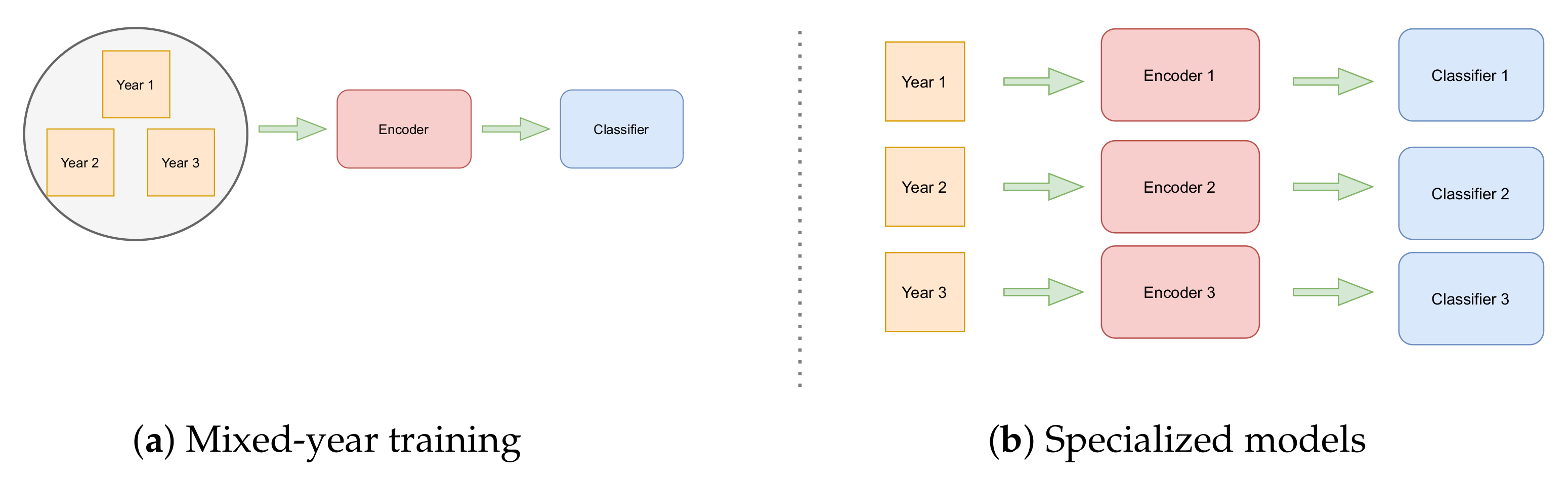
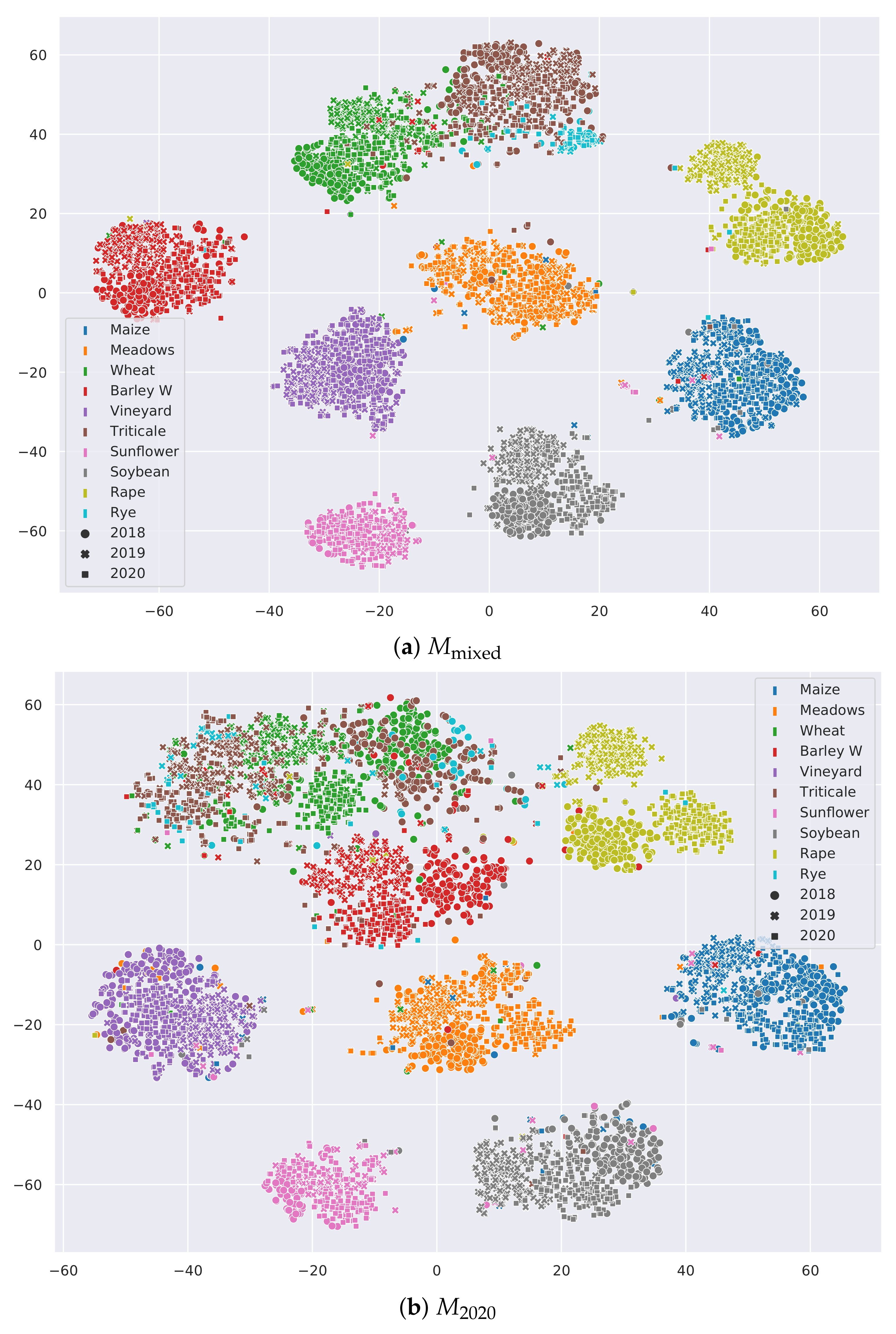
2.5.1. Mixed-Year Training

We train a single model with parcels from all available years. Our rationale is that exposing the model to data from several years will contribute to learning richer and more resilient descriptors. Indeed, each year has different meteorological conditions influencing the growth profiles of crops. Moreover, by increasing the size of the dataset, mixed-year training mitigates the negative impact of rare classes on the performance.
We assess the impact of mixed-year training by considering I = 3 specialized models whose training set is restricted to a given year: M2018, M2019, and M2020. In contrast, the model Mmixed is trained with all parcels across all years with no information regarding of the year of acquisition. All models share the same PSE+LTAE configuration [18]. We visualize the training protocols in Figure 5, and report the results in Table 2. In the rest of the paper, we use mixed year training for all models.

2.5.2. Cross-Validation

We split our data into 5 folds for cross validation. For each fold, we train on 3 folds and use the last fold for calibration and model selection, corresponding to a train/validation/test ratio of 60%, 20%, and 20% in each fold. In order to avoid data contamination and self-correlation, our folds are all spatially separated: the fold separation is done parcel-wise and not for yearly observations. A parcel cannot appear in multiple folds for different years.

2.6. Evaluation Metrics

In order to assess the performance of the different approaches evaluated, we report the Overall Accuracy (OA), corresponding to the rate of correct prediction. If we denote by N c the number of correct prediction and N the total number of parcels, the overall accuracy writes:
OA = N c N .
To address the high class imbalance, we also report the mean Intersection over Union (mIoU), defined as the unweighted class-wise average of the intersection over Union (or Jaccard distance) between the prediction and the ground truth for each class. For a given class i, IoU i is defined as the ratio between the number of elements that are both predicted and labeled by class i (the intersection, or true positives, and the number of elements that are either predicted or labeled as belonging to class i (the union). In terms of binary classification (class i vs. not class i), this translates into the following formula:
IoU i = TP i TP i + FP i + FN i ,
with TP i , FP i and FN i the number of true positives, false positives, and false negatives, respectively. The mIoU represents the average of the IoU calculated over the K studied classes:
mIoU = 1 K i = 1 K IoU i .

3. Results

In this section, we present the quantitative and qualitative impact of our design choice in terms of training protocol and architecture.

3.1. Training Protocol

Predictably, the specialized models have good performance when evaluated on a test set composed of parcels from the year they were trained, and poor results for other years, making this training procedure ill-fitted for the application at hand. In contrast, the model M mixed largely outperformed specialized models on average over the three considered years: over 15 points of mIoU. More surprisingly, the model M mixed also outperforms all specialized models even when evaluated on the year of their training set. This implies that the increased diversity of the mixed year training set allows the model to learn representations that are more robust and expressive.
In Figure 6, we illustrate the representations learned by the mixed model M mixed and the specialized model M 2020 . We remark that the parcel embeddings of the specialized model are inconsistent from one year to another, resulting in higher overlap between classes. In contrast, the mixed year model M mixed learns year-consistent representations. This results in embedding clusters with large margins between classes, illustrating the ability of the model to learn robust and discriminative SITS embeddings.

3.2. Influence of Crop Rotation Modeling

We evaluate all models presented in Section 2.3 and Section 2.4, and provide qualitative illustration in Figure 7. All models are trained with the mixed-year training protocol and only tested on parcels from the year 2020 to avoid edge effects affecting the evaluation. We give quantitative cross-validated results in Table 3. Training our model on one fold takes 4 h, and inference on all parcels takes under 3 min (over 500-parcels per second).
We observe that our model appreciably improved on the single-year model, with over 6 points gained in mIoU. The CRF models also increase the results to a lesser margin. We attribute this lesser performance to an oversmoothing phenomenon already pointed out by Bailly et al.: CRFs tends to resolve ambiguities with the most frequent transition regardless of the specificity of the observation. In contrast, our approach models simultaneously the current year’s observations and the influence of past cultivated crops. Mobs barely improves the quality of the single-year model, while this model has indeed access to more information than Msingle, the same model is used to extract SITS descriptors for all three years. This means that the model’s ambiguities and errors will be the same for all three representations, which prevent Mobs from largely improving its prediction. Our approach injects new information to the model by concatenating the labels of previous years, which is independent of the model’s limitations. Our method is more susceptible to the propagation of mistakes in the farmers’ declarations, but provides the largest increase in performance in practice.
Lastly, we concatenate both past label vectors in order to keep information about the order in which past crops were cultivated, and observe a small decrease of performance. This can be explained by the increase in model size, and we conclude that this order is not a crucial information for our model conditionally to the observation of the target year. Lastly, the performance of the model with only the declaration of the last year performs almost as well as our model with two years worth of crop declarations. This suggests that yearly transition rules are sufficient to capture most inter-year dynamics, such as permanent culture. Alternatively, our two-year scheme may suffer from sharp edge effects with only three years worth of data. Only a quantitative analysis over a longer period may resolve this ambiguity. On average, our Mdec model obtains an mIoU of 84.7% and an overall accuracy of 98.1% on the training set.
We report the confusion matrix of Mdec in Figure 8, and its performance for each crop in Table 4. We also compute Δ = IoU ( M dec ) IoU ( M single ) the gain compared to the single-year model IoU ( M single ) , as well as the ratio of improvement ρ = Δ / ( 1 mIoU ( M single ) ) . This last number indicates the proportion of IoU that have been gained by modeling crop rotations. We observe that our model provides a large performance increase across all classes but four. The improvement is particularly stark for classes with strong temporal stability such as vineyards.
In order to further this analysis, we arrange the crop types into three groups according to the crop grown in 2018 and the number of observed class successions over the 2018–2020 period:
  • Permanent Culture. Classes within this group are such that at least 90% of the observed successions are constant over three years. Contains Meadow, Vineyard, and Wood Pasture.
  • Structured Culture. A crop is said to be structured if, when grown in 2018, over 75% of the observed three year successions fall into 10 different rotations or less, and is not permanent. Contains Rapeseed, Sunflower, Soybean, Alfalfa, Leguminous, Flowers/Fruits/vegetables, and Potato.
  • Other. All other classes.
We report the unweighted class average for this three groups in Table 5. Predictably, our approach considerably improves the results for permanent cultures. Our model is also able to learn non-trivial rotations as the improvement for structured classes is also noticeable. On average, our method also improves the performance for other nonstructured classes, albeit to a lesser degree. This indicates that our model is able to learn multi-year patterns not easily captured by simple rotation statistics.

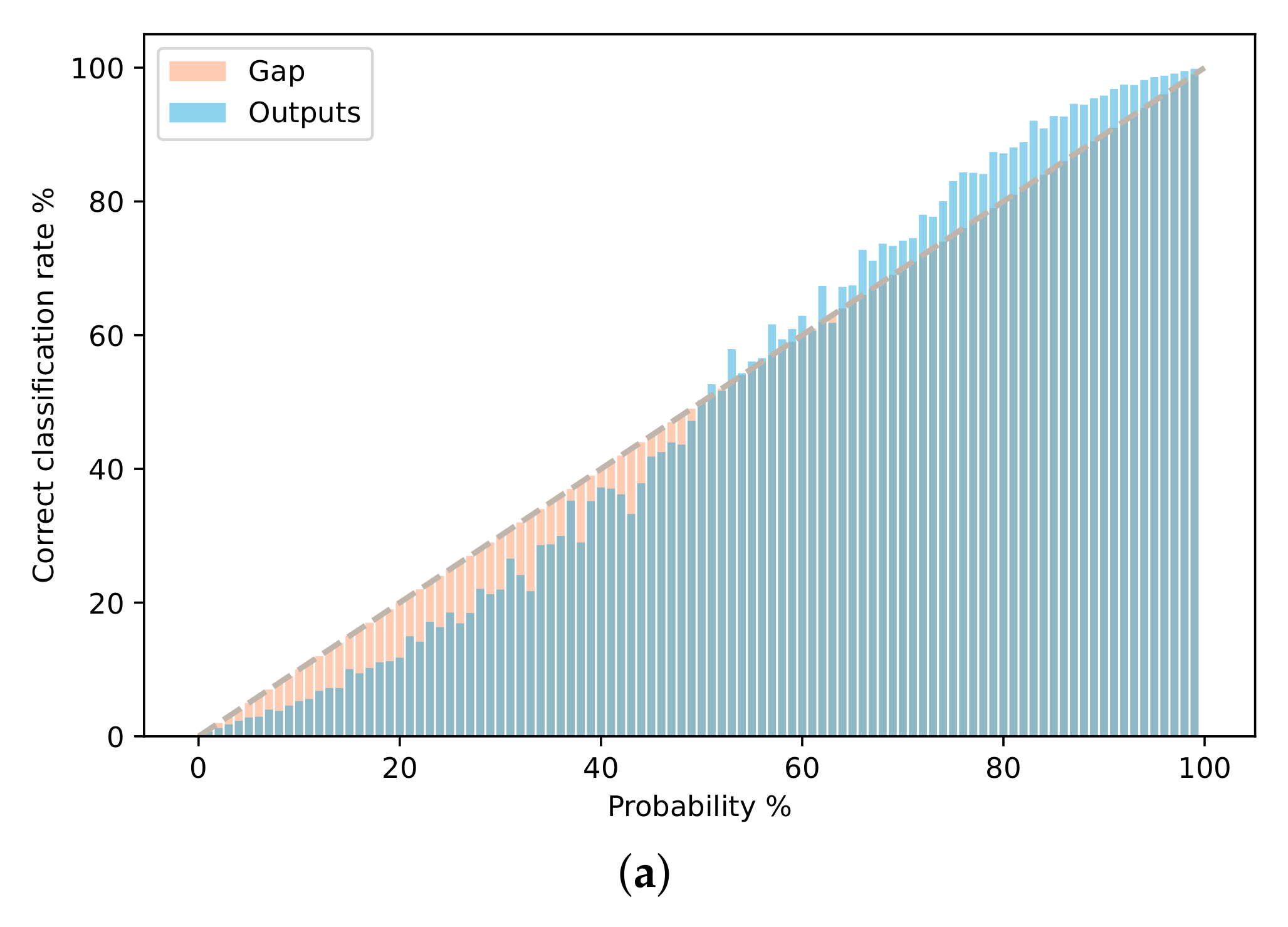
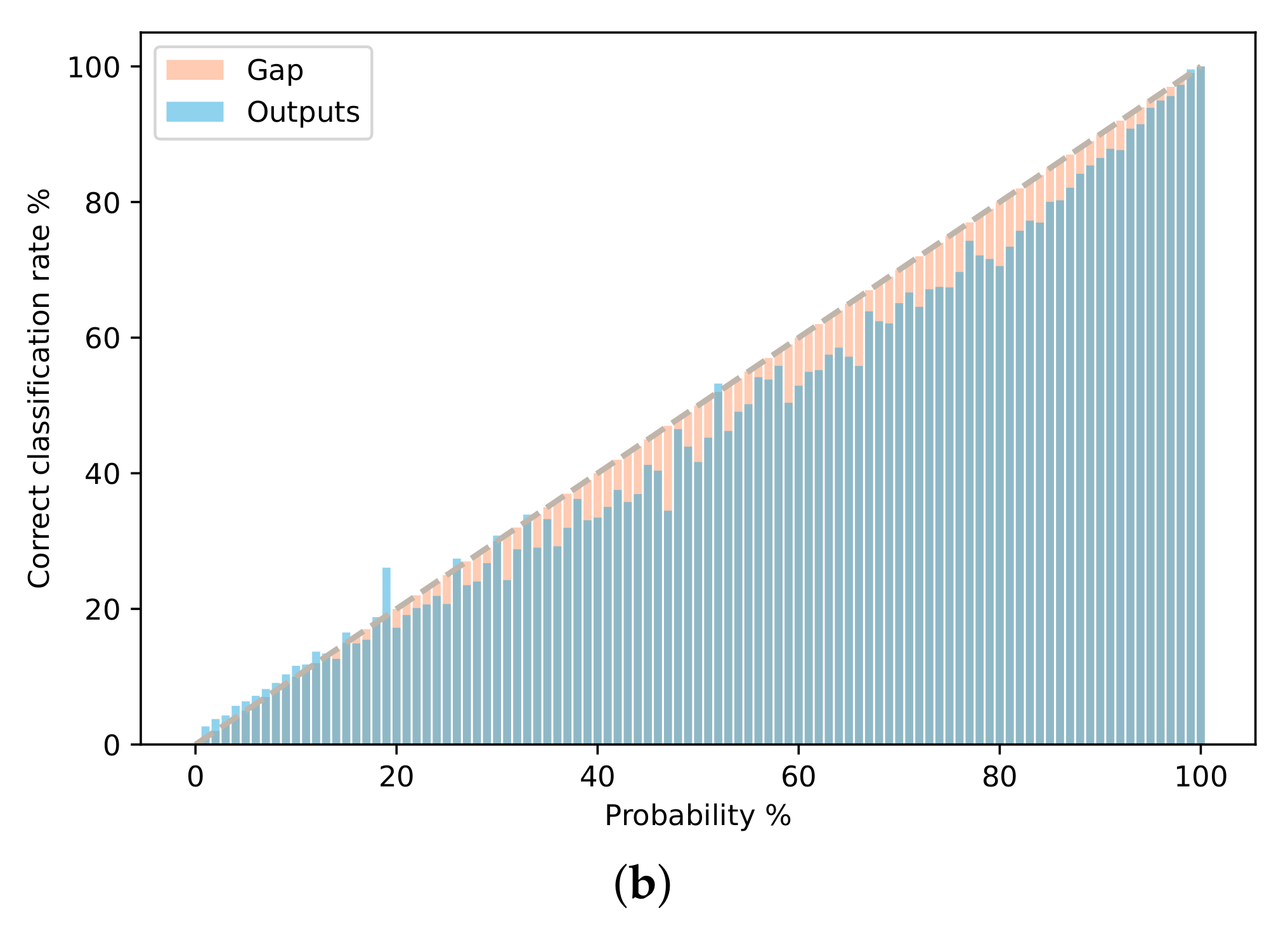
3.3. Model Calibration

Crop mapping can be used for a variety of downstream applications, such as environmental monitoring, subsidy allocation, and price prediction. These applications carry crucial economical and ecological stakes, and hence benefit from properly calibrated prediction. A prediction is said to be calibrated when the confidence (i.e., the probability associated with a given class) of the prediction corresponds to the empirical rate of correct prediction: we want 90% of the prediction with a 90% confidence to be correct. This allows for a more precise risk estimation and improves control on the rate of false positives/negatives.
Deep learning methods such as ours are notoriously badly calibrated. However, this can be corrected with the simple technique proposed by Guo et al. [40]. This method, called temperature scaling, consists of minimizing the discrepancy between the predicted confidence and the rate of errors binned into quantiles (we chose here 15 bins) on the validation set by adjusting the temperature parameters in the last softmax layer [42] (Chapter 2.4). As represented in Figure 9, we are able to improve the calibration and observe a 43% decrease of the Expected Calibration Error (ECE) at a small computation cost.

4. Discussion

In this paper, we set out to develop a deep learning method to leverage both the inter- and intra-annual dynamics of crop growth for crop mapping. We propose to enrich the learned spatio-temporal features with the last two declared cultures. Our experiments show that this simple method leads to an appreciable increase in performance compared to models operating on a single year, and that our method outperforms other approaches such as CRF smoothing or observation stacking. This improvement can be observed for most crop types, including those with rotation patterns beyond permanent culture. We now discuss the limitations of our method and of our analysis.

4.1. Choice of Backbone Network

Our method can be adapted to any network with a distinct classifier module mapping a spatio-temporal learned feature vector to a predicted vector of class scores. However, the choice of spatio-temporal encoder (backbone) is out of the scope of this article, while it may be relevant to explore the effect of our modification on other architectures, we limited our investigation to the PSE+LTAE as it is the current state-of-the-art network for crop type mapping by a large margin.

4.2. Operational Setting

We showed that training our model with samples from all available years leads to considerably improved results. However, this scenario is not compatible with the operational setting of crop monitoring, in which payment agencies may want to detect erroneous declarations before all farmers’ declarations have been received. Instead, we use the same setting than the vast majority of work in parcel classification and whose task is to classify parcels after the year is over [6,7,8,9,10,11,12,13,14,15,16,17,18,19,20].
As the Sentinel-2 mission was only operational starting in 2017, we only have access to full-year coverage since 2018. This means that, at the time of writing this paper, we only have three years worth of data. In our opinion, this prevents us from a realistic setting in which the last year is withheld from the training set. Indeed, the inter-year meteorological variations between two years are typically too great to simply test for a third year and reasonably expect good results, as corroborated with preliminary experiments not shown in this paper. As more Sentinel-2 data become available, we will be able to evaluate our approach in a more realistic setting.

4.3. Scope of the Study

Given the large amount of data involved and the complexity of data collection, we have limited our analysis and our proposed open-access dataset to a single area of the French Metropolitan territory, while nothing in our method is specific to this area, some of our analysis may be biased by the preponderance of stable cultures such as vineyards in this area. In order to confirm the generality of our conclusions, we would require a dataset with parcels taken from regions across the world with various meteorological conditions and agricultural practices. This task is made complicated by the lack of harmonization between LPIS in terms of open-access policy and even nomenclature. We hope that our results will encourage mapping agencies across the world to release multi-year LPIS in open-source to help constitute a truly global dataset, allowing the community to assess the spatial generalizability of state-of-the-art methods. We also limit ourselves to predicting the main culture in each parcel while ignoring cases with multiple growth cycles within one year. This may be particularly detrimental to its application in subtropical regions.

4.4. Applicability of Our Model

By requiring the last two grown crops to classify a parcel, our method cannot be applied to areas for which the LPIS is not easily accessible. Furthermore, our training setting requires to only select stable parcels. This can be easily obtained from the LPIS if it also contains information about the extent and position of each parcel, as is the case for the French LPIS. As a consequence, the effect of parcel with changing contours is out of the scope of our investigation.

5. Conclusions

We explored the impact of using multi-year data to improve the quality of the automatic classification of parcels from satellite image time series. We showed that training a deep learning model from multi-year observations improved its ability to generalize and resulted in across-the-board better precision. We proposed a simple modification to a state-of-the-art network in order to model both inter- and intra-year dynamics. This resulted in an increase of +6.3% of mIoU when compared to models operating on single-year data. The effect is strongest for classes with strong temporal structures, but also impact other crop types. We also showed how a simple post-processing can improve the calibration of the models considered.
Finally, we release both our code and our data. We hope that our promising results will encourage the SITS community to develop methods modeling multiple time scales simultaneously, and to release more datasets spanning several years.

Author Contributions

Software, data curation, writing—original draft preparation, and visualization: F.Q.; methodology, conceptualization, validation, formal analysis, and investigation: F.Q. and L.L.; supervision, resources, writing—review and editing, project administration, funding acquisition: L.L. All authors have read and agreed to the published version of the manuscript.

Funding

This research was funded by the French Payment Agency ASP.

Data Availability Statement

The codes and datasets are available at https://github.com/felixquinton1/deep-crop-rotation, (accessed on 11 November 2021) for the codes and https://zenodo.org/record/5535882, (accessed on 11 November 2021) for the dataset.

Acknowledgments

We thanks the SIMV department of IGN for their logistic support and data expertise. We thank the ASP for their continuous expertise and for initiating this project. The satellite images were gathered by THEIA: “Value-added data processed by the CNES for the Theia data cluster using Copernicus data. The treatments use algorithms developed by Theia’s Scientific Expertise Centres”.

Conflicts of Interest

The authors declare no conflict of interest.

Abbreviations

The following abbreviations are used in this manuscript:
CNNConvolutional Neural Network
MLPMulti Layer Perceptron
RNNRecurrent Neural Network
PSEPixel Set encoder
TAETemporal Attention Encoder
LTAELightweight Temporal Attention Encodeur
ECEExpected Calibration Error
CAPCommon Agricultural Policy
LPISLand-Parcel Identification System
SITSSatellite Image Time Series
CRFConditional Random Fields

References

  1. The Common Agricultural Policy at a Glance. Available online: https://ec.europa.eu/info/food-farming-fisheries/key-policies/common-agricultural-policy/cap-glance_en (accessed on 24 September 2021).
  2. Loudjani, P.; Devos, W.; Baruth, B.; Lemoine, G. Artificial Intelligence and EU Agriculture. 2020. Available online: https://marswiki.jrc.ec.europa.eu/wikicap/images/c/c8/JRC-Report_AIA_120221a.pdf (accessed on 10 October 2021).
  3. Koetz, B.; Defourny, P.; Bontemps, S.; Bajec, K.; Cara, C.; de Vendictis, L.; Kucera, L.; Malcorps, P.; Milcinski, G.; Nicola, L.; et al. SEN4CAP Sentinels for CAP monitoring approach. In Proceedings of the JRC IACS Workshop, Valladolid, Spain, 10–11 April 2019. [Google Scholar]
  4. Drusch, M.; Del Bello, U.; Carlier, S.; Colin, O.; Fernandez, V.; Gascon, F.; Hoersch, B.; Isola, C.; Laberinti, P.; Martimort, P.; et al. Sentinel-2: ESA’s optical high-resolution mission for GMES operational services. Remote Sens. Environ. 2012, 120, 25–36. [Google Scholar] [CrossRef]
  5. Registre Parcellaire Graphique (RPG): Contours des Parcelles et îlots Culturaux et Leur Groupe de Cultures Majoritaire. Available online: https://www.data.gouv.fr/en/datasets/registre-parcellaire-graphique-rpg-contours-des-parcelles-et-ilots-culturaux-et-leur-groupe-de-cultures-majoritaire/ (accessed on 24 September 2021).
  6. Garnot, V.S.F.; Landrieu, L.; Giordano, S.; Chehata, N. Satellite image time series classification with pixel-set encoders and temporal self-attention. In Proceedings of the IEEE/CVF Conference on Computer Vision and Pattern Recognition (CVPR), Seattle, WA, USA, 13–19 June 2020. [Google Scholar]
  7. Pelletier, C.; Webb, G.I.; Petitjean, F. Deep learning for the classification of Sentinel-2 image time series. In Proceedings of the IGARSS 2019—2019 IEEE International Geoscience and Remote Sensing Symposium, Yokohama, Japan, 28 July–2 August 2019. [Google Scholar]
  8. Rußwurm, M.; Körner, M. Self-attention for raw optical satellite time series classification. ISPRS J. Photogramm. Remote Sens. 2020, 169, 421–435. [Google Scholar] [CrossRef]
  9. Zheng, B.; Myint, S.W.; Thenkabail, P.S.; Aggarwal, R.M. A support vector machine to identify irrigated crop types using time-series Landsat NDVI data. Int. J. Appl. Earth Obs. Geoinf. 2015, 34, 103–112. [Google Scholar] [CrossRef]
  10. Vuolo, F.; Neuwirth, M.; Immitzer, M.; Atzberger, C.; Ng, W.T. How much does multi-temporal Sentinel-2 data improve crop type classification? Int. J. Appl. Earth Obs. Geoinf. 2018, 72, 122–130. [Google Scholar] [CrossRef]
  11. Siachalou, S.; Mallinis, G.; Tsakiri-Strati, M. A hidden Markov models approach for crop classification: Linking crop phenology to time series of multi-sensor remote sensing data. Remote Sens. 2015, 7, 3633–3650. [Google Scholar] [CrossRef] [Green Version]
  12. Belgiu, M.; Csillik, O. Sentinel-2 cropland mapping using pixel-based and object-based time-weighted dynamic time warping analysis. Remote Sens. Environ. 2018, 204, 509–523. [Google Scholar] [CrossRef]
  13. Kussul, N.; Lavreniuk, M.; Skakun, S.; Shelestov, A. Deep learning classification of land cover and crop types using remote sensing data. Geosci. Remote Sens. Lett. 2017, 14, 778–782. [Google Scholar] [CrossRef]
  14. Garnot, V.S.F.; Landrieu, L.; Giordano, S.; Chehata, N. Time-Space tradeoff in deep learning models for crop classification on satellite multi-spectral image time series. In Proceedings of the IGARSS 2019—2019 IEEE International Geoscience and Remote Sensing Symposium, Yokohama, Japan, 28 July–2 August 2019. [Google Scholar]
  15. Rußwurm, M.; Körner, M. Multi-temporal land cover classification with sequential recurrent encoders. ISPRS Int. J.-Geo-Inf. 2018, 7, 129. [Google Scholar] [CrossRef] [Green Version]
  16. Yuan, Y.; Lin, L. Self-Supervised Pretraining of Transformers for Satellite Image Time Series Classification. J. Sel. Top. Appl. Earth Obs. Remote Sens. 2020, 14, 474–487. [Google Scholar] [CrossRef]
  17. Kondmann, L.; Toker, A.; Rußwurm, M.; Unzueta, A.C.; Peressuti, D.; Milcinski, G.; Mathieu, P.P.; Longépé, N.; Davis, T.; Marchisio, G.; et al. DENETHOR: The DynamicEarthNET dataset for Harmonized, inter-Operable, analysis-Ready, daily crop monitoring from space. In Proceedings of the 35th Conference on Neural Information Processing Systems (NeurIPS 2021), Virtual, 6–14 December 2021. [Google Scholar]
  18. Garnot, V.S.F.; Landrieu, L. Lightweight temporal self-attention for classifying satellite images time series. In International Workshop on Advanced Analytics and Learning on Temporal Data; Springer: Berlin/Heidelberg, Germany, 2020. [Google Scholar]
  19. Schneider, M.; Körner, M. [Re] Satellite Image Time Series Classification with Pixel-Set Encoders and Temporal Self-Attention. In ML Reproducibility Challenge 2020; 2020; Available online: https://openreview.net/forum?id=r87dMGuauCl (accessed on 10 October 2021).
  20. Garnot, V.S.F.; Landrieu, L. Panoptic Segmentation of Satellite Image Time Series with Convolutional Temporal Attention Networks. In Proceedings of the IEEE/CVF International Conference on Computer Vision, Montreal, QC, Canada, 11–17 October 2021. [Google Scholar]
  21. Dury, J.; Schaller, N.; Garcia, F.; Reynaud, A.; Bergez, J.E. Models to support cropping plan and crop rotation decisions. A review. Agron. Sustain. Dev. 2012, 32, 567–580. [Google Scholar] [CrossRef] [Green Version]
  22. Dogliotti, S.; Rossing, W.; Van Ittersum, M. ROTAT, a tool for systematically generating crop rotations. Eur. J. Agron. 2003, 19, 239–250. [Google Scholar] [CrossRef]
  23. Myers, K.; Ferguson, V.; Voskoboynik, Y. Modeling Crop Rotation with Discrete Mathematics. One-Day Sustainability Modules for Undergraduate Mathematics Classes. DIMACS. Available online: http://dimacs.rutgers.edu/MPE/Sustmodule.html (accessed on 11 March 2015).
  24. Brankatschk, G.; Finkbeiner, M. Modeling crop rotation in agricultural LCAs—Challenges and potential solutions. Agric. Syst. 2015, 138, 66–76. [Google Scholar] [CrossRef]
  25. Detlefsen, N.K.; Jensen, A.L. Modelling optimal crop sequences using network flows. Agric. Syst. 2007, 94, 566–572. [Google Scholar] [CrossRef]
  26. Aurbacher, J.; Dabbert, S. Generating crop sequences in land-use models using maximum entropy and Markov chains. Agric. Syst. 2011, 104, 470–479. [Google Scholar] [CrossRef]
  27. Bachinger, J.; Zander, P. ROTOR, a tool for generating and evaluating crop rotations for organic farming systems. Eur. J. Agron. 2007, 26, 130–143. [Google Scholar] [CrossRef]
  28. Schönhart, M.; Schmid, E.; Schneider, U.A. CropRota—A crop rotation model to support integrated land use assessments. Eur. J. Agron. 2011, 34, 263–277. [Google Scholar] [CrossRef]
  29. Levavasseur, F.; Martin, P.; Bouty, C.; Barbottin, A.; Bretagnolle, V.; Thérond, O.; Scheurer, O.; Piskiewicz, N. RPG Explorer: A new tool to ease the analysis of agricultural landscape dynamics with the Land Parcel Identification System. Comput. Electron. Agric. 2016, 127, 541–552. [Google Scholar] [CrossRef]
  30. Kollas, C.; Kersebaum, K.C.; Nendel, C.; Manevski, K.; Müller, C.; Palosuo, T.; Armas-Herrera, C.M.; Beaudoin, N.; Bindi, M.; Charfeddine, M.; et al. Crop rotation modelling—A European model intercomparison. Eur. J. Agron. 2015, 70, 98–111. [Google Scholar] [CrossRef]
  31. Osman, J.; Inglada, J.; Dejoux, J.F. Assessment of a Markov logic model of crop rotations for early crop mapping. Comput. Electron. Agric. 2015, 113, 234–243. [Google Scholar] [CrossRef] [Green Version]
  32. Giordano, S.; Bailly, S.; Landrieu, L.; Chehata, N. Improved Crop Classification with Rotation Knowledge using Sentinel-1 and-2 Time Series. Photogramm. Eng. Remote Sens. 2018, 86, 431–441. [Google Scholar] [CrossRef]
  33. Bailly, S.; Giordano, S.; Landrieu, L.; Chehata, N. Crop-rotation structured classification using multi-source Sentinel images and lpis for crop type mapping. In Proceedings of the IGARSS 2018—2018 IEEE International Geoscience and Remote Sensing Symposium, Valencia, Spain, 22–27 July 2018. [Google Scholar]
  34. Yaramasu, R.; Bandaru, V.; Pnvr, K. Pre-season crop type mapping using deep neural networks. Comput. Electron. Agric. 2020, 176, 105664. [Google Scholar] [CrossRef]
  35. Multi-Year Dataset. Available online: https://zenodo.org/record/5535882 (accessed on 10 October 2021). [CrossRef]
  36. Baghdadi, N.; Leroy, M.; Maurel, P.; Cherchali, S.; Stoll, M.; Faure, J.F.; Desconnets, J.C.; Hagolle, O.; Gasperi, J.; Pacholczyk, P. The Theia land data centre. In Proceedings of the Remote Sensing Data Infrastructures (RSDI) International Workshop, La Grande Motte, France, 1 October 2015. [Google Scholar]
  37. Qi, C.R.; Su, H.; Mo, K.; Guibas, L.J. Pointnet: Deep learning on point sets for 3d classification and segmentation. In Proceedings of the IEEE Conference on Computer Vision and Pattern Recognition (CVPR), Honolulu, HI, USA, 21–26 July 2017; pp. 652–660. [Google Scholar]
  38. Vaswani, A.; Shazeer, N.; Parmar, N.; Uszkoreit, J.; Jones, L.; Gomez, A.N.; Kaiser, L.; Polosukhin, I. Attention is all you need. In Proceedings of the 31st Conference on Neural Information Processing Systems (NIPS 2017), Long Beach, CA, USA, 4–9 December 2017. [Google Scholar]
  39. Wainwright, M.J.; Jordan, M.I. Graphical Models, Exponential Families, and Variational Inference; Now Publishers Inc.: Norwell, MA, USA, 2008. [Google Scholar]
  40. Guo, C.; Pleiss, G.; Sun, Y.; Weinberger, K.Q. On calibration of modern neural networks. In Proceedings of the ICML International Conference on Machine Learning, Sydney, Australia, 6–11 August 2017. [Google Scholar]
  41. Schütze, H.; Manning, C.D.; Raghavan, P. Introduction to Information Retrieval; Cambridge University Press: Cambridge, UK, 2008; Volume 39. [Google Scholar]
  42. Bishop, C.M. Pattern Recognition and Machine Learning; Springer: Berlin/Heidelberg, Germany, 2006. [Google Scholar]
Figure 1. Multi-Year Sentinel-2 Data. Details of our area of interest for the three years studied in this article. The crop type of each parcel is represented by the color of a polygon following their contour according to the legend above. This color code is used throughout this article for all figures representing cultivated crops.
Remotesensing 13 04599 g001
Figure 2. Area of Interest. The studied parcels are taken from the 31TFM Sentinel-2 tile, covering an area of 110 × 110 km and containing over 103,602 parcels meeting our size, shape, and stability criteria. (a) Large view of the tile. (b) Detail of the area.
Remotesensing 13 04599 g002
Figure 3. Intra-Year Dynamics. Evolution of two areas across three seasons of the year 2020. The top parcels contains mainly meadow parcels, while the bottom one comprises more diverse crops. The aspect of most parcel drastically changes across one year’s worth of acquisition, corresponding to different phases in the growth cycle. (a) Winter. (b) Spring. (c) Summer.
Remotesensing 13 04599 g003
Figure 4. Multi-Year Modeling. Different approaches to model crop rotation dynamics: (a) the model only has access to the current year’s observation; (b) a chain-CRF is used to model the influence of past cultivated crop; (c) the model has access to the observation of the past two years; (d) proposed approach: the model has access to the last two declared crops.
Remotesensing 13 04599 g004
Figure 5. Training Protocol. A single model is trained with parcels taken from all three years (a), and three specialized models whose training set only comprises observation for a given year (b).
Remotesensing 13 04599 g005
Figure 6. Learned Representations. Illustrations of the learned SITS representations of the mixed-year model Mmixed (a) and the specialized M2020 (b). T-SNE algorithm is used to plot in 2D the representation for 100 parcels over 10 classes and 3 years. We observe that Mmixed produced cluster of embeddings that are consistent from one year to another, and with clearer demarcation between classes.
Remotesensing 13 04599 g006
Figure 7. Qualitative Illustration. Detail of the area of interest with the ground truth in (a) and the qualification of the prediction in (b) with correct prediction in blue and errors in red.
Remotesensing 13 04599 g007
Figure 8. Confusion Matrix. Confusion matrix of the prediction of M dec for the year 2020. The area of each entry corresponds to the square root of the number of predictions.
Remotesensing 13 04599 g008
Figure 9. Model calibration. Empirical rate of correct prediction by predicted confidence. We quantize the predicted confidence into 100 bins for visualization purposes. For a perfectly calibrated prediction, the blue histogram would exactly follow the orange line. We observe that a simple post-processing step can considerably improves calibration. (a) No calibration, ECE = 1.4%. (b) Calibration, ECE = 0.8%.
Remotesensing 13 04599 g009aRemotesensing 13 04599 g009b
Table 1. Crop distribution. We indicate the number of parcels declarations in the LPIS for each class across all 103,602 parcels and all 3 years.
ClassCountClassCount
Meadow184,489Triticale5114
Maize42,006Rye569
Wheat27,921Rapeseed7624
Barley Winter10,516Sunflower1886
Vineyard15,461Soybean6072
Sorghum820Alfalfa2682
Oat Winter529Leguminous1454
Mixed cereal1061Flo./fru./veg.1079
Oat Summer330Potato230
Barley Summer538Wood pasture425
Table 2. Quantitative evaluation. Performance (mIoU and OA) of the different specialized models M 2018 , M 2019 , M 2020 and of the mixed-years model M mixed evaluated on each year individually and all available years simultaneously with 5-fold cross-validation. The best performances are shown in bold. Boxed values correspond to evaluations where the training set and the evaluation set are drawn from the same year. The mixed-year model performs better for all years, even compared to specialized models.
Model 2018 2019 2020 3 Years
OAmIoU OAmIoU OAmIoU OAmIoU
M 2018 97.064.7 90.345.5 90.843.4 92.749.1
M 2019 88.939.5 97.270.1 88.740.1 91.648.0
M 2020 91.444.2 93.751.8 96.767.3 93.954.0
M mixed 97.369.2 97.472.2 96.868.7 97.270.4
Table 3. Performance by model. Performances (mIoU and OA) of the models Msingle, Mobs, MCRF, and Mdec tested for the year 2020. Our proposed model Mdec achieve higher performance than Msingle with a 6.3% mIoU gap.
ModelDescriptionOAmIoU
M sin gle single-year observation96.868.7
M obs bypassing 2 years of observation96.869.3
M CRF using past 2 declarations in a CRF96.872.3
Mdec-one-yearconcatenating last declaration only97.574.3
Mdec-concatconcatenating past 2 declarations97.574.4
M dec proposed method97.575.0
Table 4. Performance by class. IoU per class of our model Mdec for the year 2020, as well as the improvement Δ compared to the single-year model Msingle, and the ratio of improvement ρ. All values are given in %, and we sort the classes according to decreasing ρ.
ClassIoU Δ ρ ClassIoU Δ ρ
Wood Pasture92.4+48.286.3Oat Summer52.8+3.67.0
Vineyard99.3+1.468.7Rapeseed98.3+0.16.6
Alfalfa68.7+23.949.9Maize95.7+0.26.3
Flo./Fru./Veg.83.4+14.546.5Wheat91.9+0.33.9
Meadow98.4+0.936.9Barley Summer64.3+1.13.1
Leguminous45.2+14.621.1Potato57.1+0.51.2
Rye54.7+6.412.4Sunflower92.2−0.1−0.3
Oat Winter57.7+4.59.7Sorghum56.6−0.2−0.4
Triticale68.72.67.8Soybean91.8−0.2−3.1
Mix. Cereals31.0+5.16.8Barley Winter92.8−0.6−8.5
Table 5. Improvement Relative to Structure. Classwise IoU and mean improvement of our model compared to the single-year model according to the rotation structure of the cultivated crops.
CategorymIoUMean Δ
Permanent97.316.9
Structured77.77.6
Other66.62.3
Publisher’s Note: MDPI stays neutral with regard to jurisdictional claims in published maps and institutional affiliations.

