A 3D Compensation Method for the Systematic Errors of Kinect V2

Abstract

To reduce the 3D systematic error of the RGB-D camera and improve the measurement accuracy, this paper is the first to propose a new 3D compensation method for the systematic error of a Kinect V2 in a 3D calibration field. The processing of the method is as follows. First, the coordinate system between the RGB-D camera and 3D calibration field is transformed using 3D corresponding points. Second, the inliers are obtained using the Bayes SAmple Consensus (BaySAC) algorithm to eliminate gross errors (i.e., outliers). Third, the parameters of the 3D registration model are calculated by the iteration method with variable weights that can further control the error. Fourth, three systematic error compensation models are established and solved by the stepwise regression method. Finally, the optimal model is selected to calibrate the RGB-D camera. The experimental results show the following: (1) the BaySAC algorithm can effectively eliminate gross errors; (2) the iteration method with variable weights could better control slightly larger accidental errors; and (3) the 3D compensation method can compensate 91.19% and 61.58% of the systematic error of the RGB-D camera in the depth and 3D directions, respectively, in the 3D control field, which is superior to the 2D compensation method. The proposed method can control three types of errors (i.e., gross errors, accidental errors and systematic errors) and model errors and can effectively improve the accuracy of depth data.

1. Introduction

The second version of the Microsoft Kinect (i.e., Kinect V2) is an RGB-D camera based on time of flight (TOF) technology for depth measurement that can capture color and depth images simultaneously. Compared with Kinect V1, Kinect V2 can obtain more accurate depth data and better-quality point cloud data [1]. With its advantages of being portable, low cost [2], highly efficient [3] and robust [4], this device has been widely applied in computer vision [5,6], medicine [7,8], target and posture recognition [9,10], robot localization and navigation [11,12], 3D reconstruction [13,14,15], etc. Recently, with the continuous upgrading of sensors, camera devices have evolved from RGB cameras to RGB-D cameras that can acquire 3D information. Thus, the detectable range has been extended from the 2D plane to 3D space. The calibration of RGB-D cameras and their application in 3D indoor scene reconstruction have gradually attracted attention [16]. However, the depth camera data include some random errors and systematic errors that lead to problems such as the deviation and distortion of RGB-D cameras [17], which makes the data accuracy unfit for meeting the needs of research and application in high accuracy 3D reconstruction. Therefore, it is of great significance to study the calibration and error compensation of RGB-D cameras.

The purpose of camera calibration is to acquire the parameters of the camera imaging model, including the intrinsic parameters that characterize the intrinsic structure of the camera and the optical characteristics of the lens and the external parameters that describe the spatial pose of the camera [18]. Moreover, camera calibration methods can be roughly divided into four categories: laboratory calibration [19], optical calibration [20], on-the-job calibration [21], and self-calibration [22]. The calibration field in laboratory calibration is generally composed of some control points with known spatial coordinates, and it can also be subdivided into a 2D calibration field and a 3D calibration field.

Because of its simplicity and portability, the 2D calibration field has been widely used in studies about close range camera calibration [23]. For instance, Zhang [24] used regular checkerboard photos taken at different angles obtained from the 2D calibration field, then extracted feature points and obtained the intrinsic and external parameters and distortion coefficient of the RGB camera based on specific geometric relations. Sturm [25] proposed an algorithm that can calibrate different views from a camera with variable intrinsic parameters simultaneously, and it is easy to incorporate known values of intrinsic parameters in the algorithm. Boehm and Pattinson [26] proposed calibrating the intrinsic and external parameters of a ToF camera based on a checkerboard. Liu et al. [27] applied two different algorithms to calibrate a Kinect color camera and depth camera, respectively, and then developed a model that could calibrate two cameras concurrently. Song et al. [28] utilized a checkerboard with a hollow block to measure the deviation and camera parameters, and the method produced significantly better accuracy, even if there was noise within the depth data.

The layout conditions of the 3D calibration field are more complex and difficult than those of the 2D calibration field, so there are few studies on the calibration of depth cameras based on it. However, the 3D calibration field contains rich 3D information, especially depth information, which could preferably suit the needs of depth camera calibration in 3D coordinate space. Therefore, the 3D calibration field has great potential to further improve the depth camera calibration accuracy in theory and practice. Some scholars explored the following issues. Gui et al. [29] obtained accurate intrinsic parameters and the relative attitude of two cameras using a simple 3D calibration field, and the iterative closest point (ICP) method was used to solve the polynomial model for correcting the depth error. Zhang [30] established the calibration model of a Kinect V2 depth camera in a 3D control field based on collinearity equations and spatial resection to correct the depth and calibrate the relative pose, which provided an idea for further improving the calibration accuracy of an RGB-D camera.

In conclusion, the 3D (i.e., XOY plane and Z depth) error compensation method for Kinect V2 could be further developed and improved in the following aspects:

(1)

Multiple types of error control: some studies are only concerned with one type or two types of error in depth camera data while the other errors are ignored. For example, some of the aforementioned compensation models ignore processing the potential model errors, resulting in inaccurate systematic error compensation.

(2)

Model error control: research based on the 3D calibration field needs to be supplemented, and a higher accuracy 3D error compensation model for an RGB-D camera needs to be explored.

In order to solve the above two problems, based on an indoor 3D calibration field, we propose a new 3D error compensation method for the systematic error of a Kinect V2 depth camera for the first time. This paper has the following innovations and contributions:

(1)

A new method to simultaneously handle three types of errors in RGB-D cameras is the first to be proposed. First, the Bayes SAmple Consensus (BaySAC) is used to eliminate the gross errors generated in RGB-D camera processing. Then, the potential slightly larger accidental errors are further controlled by the iteration method with variable weights. Finally, a new optimal model is established to compensate for the systematic error. Therefore, the proposed method can simultaneously control the gross error, accidental error, and systematic error in RGB-D camera (i.e., Kinect V2) calibration.

(2)

3D systematic error compensation models of a Kinect V2 depth camera based on a strict 3D calibration field are established and optimized for the first time. A stepwise regression is used to optimize the parameters of these models. Then, the optimal model is selected to compensate the depth camera, which reduces the error caused by improper model selection, i.e., the model error or overparameterization problem of the model.

2. Materials and Methods

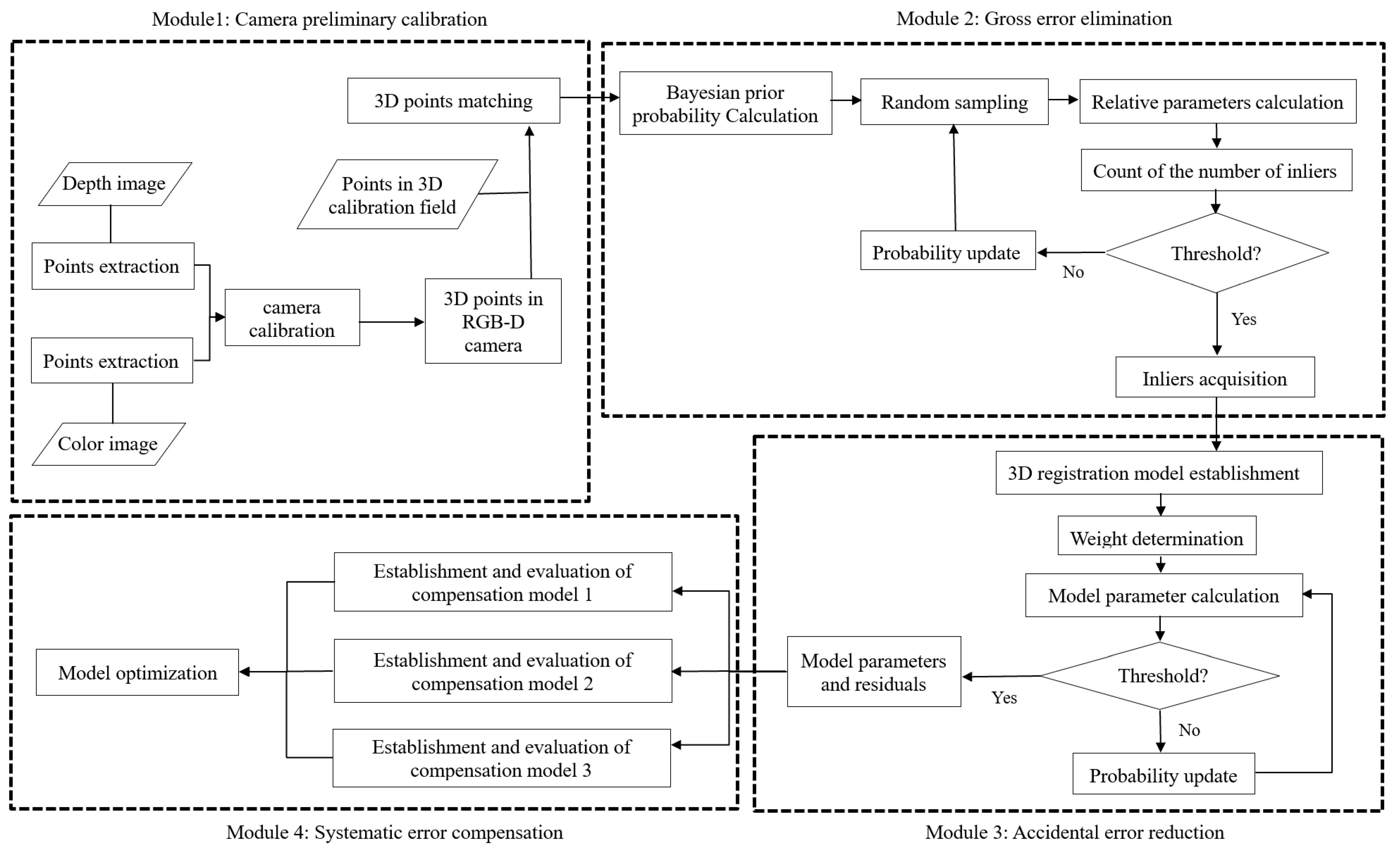
2.1. Algorithm Processing Flow

The algorithm is divided into four modules. In module 1, the initial RGB-D camera calibration is pre-processed to obtain depth error data. Module 2 acquires the inliers and eliminates the gross errors (i.e., outliers). Module 3 controls slightly larger accidental errors for the parameters of the 3D transformation model. Module 4 selects the optimal model to compensate for the systematic error of the RGB-D camera. The specific algorithm processing is as follows (Figure 1).

(1)

Acquire the raw image data. Color images and depth images are taken from an indoor 3D calibration field, and then corresponding points are extracted separately.

(2)

Preprocess RGB-D data. The subpixel-accurate 2D coordinates of the marker points [31] on the color image and the corresponding depth image are extracted and transformed to acquire 3D points in the RGB-D camera coordinate system.

(3)

Match the 3D point pairs. The marker points from the 3D calibration field and RGB-D camera are matched to acquire 3D corresponding point pairs, which are used to calculate the depth error.

(4)

Obtain inliers. The inliers are determined by BaySAC, thus, gross errors are eliminated.

(5)

Compute the parameters of the 3D transformation model based on inliers. The iteration method with variable weights is used to compute the model parameters, and residuals with slightly larger accidental errors are controlled.

(6)

Establish 3D compensation models of the systematic error. Three types of error compensation models are established, and the parameters of these models are calculated by the stepwise regression method to avoid overparameterization.

(7)

Select the optimal model to compensate for the systematic error. The accuracy of the models is evaluated, and then the optimal model is selected to calibrate the RGB-D camera.

2.2. Data Acquisition and Preprocessing of an RGB-D Camera

The high accuracy indoor 3D camera calibration field in Figure 2a was established by the School of Remote Sensing and Information Engineering, Wuhan University. It contains many control points with known coordinates. The coordinates of these points were measured by a high accuracy electronic total station, the measurement accuracy of which could reach 0.2 mm.

A Kinect V2 depth camera was used to collect data; and the software development kit (SDK) driver of Kinect 2.0 was used to take 11 sets of images from different angles, including the color images in Figure 2b and the depth images in Figure 2c. Some effective measures are taken to reduce the random errors that exist in the depth data and improve the quality of the raw error data. For example, when we shoot an RGB-D image in a 3D calibration field, the influence of ambient light could be reduced by keeping the intensity of the ambient light in an appropriate range. In addition, to decrease the influence of temperature on the depth measurement accuracy, the camera is turned off at regular intervals and then continues to shoot after the depth sensor cools down. Moreover, the Kinect V2 is kept relatively motionless during the measurement to reduce motion blur.

Then, the marker point pairs in two types of images were extracted in MATLAB [31], and the coordinates of the points in the color images were 2D coordinates. Then, the method need to combine the depth values in the depth image with the 2D coordinates in the RGB image of the corresponding points to acquire the 3D coordinates of the observation points.

The observation points of the RGB-D camera in Figure 3a were matched with the corresponding control points in the 3D calibration field in Figure 3b. Then, the coordinates of the more accurate control points were taken as true values to be compared with the observation points from the RGB-D camera so as to compute the initial camera residual. However, the coordinate system of the 3D calibration field is inconsistent with that of the depth camera. Hence, before 3D point pairs are applied to calculate the 3D systematic error, it is necessary to achieve the 3D coordinate transformation.

2.3. 3D Coordinate Transformation Relationship

Camera calibration finds the transformation model between the camera space and the object space [32] and calculates the parameters of the camera imaging model [24]. We suppose P_c= (X_c,Y_c,Z_c,1)^T is the homogeneous coordinates of a 3D point in the RGB-D camera coordinate system, and its corresponding homogeneous coordinate in the world coordinate system is P_w= (X_w,Y_w,Z_w,1)^T. There are rotations, translations, and scale variations between them. According to the pinhole model [32], the coordinate transformation can be achieved by the following formulas:

$$\left[\begin{array}{c}{X}_c\\ Y_c\\ Z_c\\ 1\end{array}\right]=s\left[\begin{array}{cccc}{R}_{11}& R_{12}& R_{13}& T_x\\ R_{21}& R_{22}& R_{23}& T_y\\ R_{31}& R_{32}& R_{33}& T_z\\ 0& 0& 0& 1/s\end{array}\right]\left[\begin{array}{c}{X}_w\\ Y_w\\ Z_w\\ 1\end{array}\right]$$

(1)

$$R=\left[\begin{array}{ccc}{R}_{11}& R_{12}& R_{13}\\ R_{21}& R_{22}& R_{23}\\ R_{31}& R_{32}& R_{33}\end{array}\right]$$

(2)

$$\mathit{T}={\left[\begin{array}{ccc}Tx& Ty& Tz\end{array}\right]}^{\mathrm{T}}$$

(3)

where R is a rotation matrix; T is a translation vector; and s is the scaling factor in the depth image. R and T are the matrix and vector of the external parameters of the camera, respectively.

Under the condition that the camera is not shifted or rotated, the camera coordinates and image coordinates could be transformed to each other. This is realized by Formula (4). The error compensation model proposed in this paper is based on image coordinates (x, y) and depth value d.

$$\left[\begin{array}{c}x\\ y\\ d\\ 1\end{array}\right]=\left[\begin{array}{cccc}{f}_x/Z_c& 0& 0& c_x\\ 0& f_y/Z_c& 0& c_y\\ 0& 0& s& 0\\ 0& 0& 0& 1\end{array}\right]\left[\begin{array}{c}{X}_c\\ Y_c\\ Z_c\\ 1\end{array}\right]$$

(4)

where f_x and f_y represent the focal lengths of the camera; (c_x, c_y) is the aperture center; and s is the scaling factor in the depth image.

2.4. Inlier Determination Based on BaySAC

The gross errors in the depth data required by the Kinect V2 has an impact on the effects of 3D coordinate transformation; thus, we adopt the optimized BaySAC as proposed by Kang [33] to eliminate them. BaySAC is an improved random sample consensus (RANSAC) algorithm [34]. The Bayesian prior probability is used to reduce the number of iterations by half in some cases and improve the performance of the algorithm effectively to eliminate outliers, which makes BaySAC significantly superior to other sampling algorithms [35]. The procedure of the algorithm is as follows:

(1)

Calculate the maximum number of iterations K using Formula (5):

$$K=\frac{log(1-p)}{log(1-w^n)}$$

(5)

where w is the assumed percentage of inliers with respect to the total number of points in the dataset; and the significance level p represents the probability that n (the model proposed in this paper needs at least 4 point pairs, so n is greater than or equal to 4) points selected from the dataset to solve the model parameters in multiple iterations are all inliers.

In general, the value of w is uncertain, so it can be estimated as a relatively small number to acquire the expected set of inliers with a moderate number of iterations. Therefore, we initially estimate that w is approximately 80% in this experiment. The significance level p should be less than 0.05 to ensure that the selected points are inliers in the iteration.

(2)

Determine the Bayesian prior probability $P_{\left(X_w,Y_w,Z_w\right)}$ of any 3D control point using Formula (6) as follows:

$$P_{(X_w,Y_w,Z_w)}=1-\frac{\sqrt{{(\Delta X)}^2+{(\Delta Y)}^2+{(\Delta Z)}^2}}{\sqrt{X_w{}^2+Y_w{}^2+Z_w{}^2}}$$

(6)

where P_(Xw,Yw,Zw) is a probability; and (ΔX,ΔY,ΔZ) represents the deviation between the 3D point and its transformed correspondence. If the sum of squares ΔX, ΔY and ΔZ is smaller, it means that the above deviation is smaller and it is more reliable; and if the sum of squares X_w, Y_w and Z_w is larger, it means that the point is closer to the borders of the 3D points set, so these points are better for 3D similarity transformation.

(3)

Compute the parameters of the hypothesis model. From the measurement point set, n points with the highest inlier probabilities are selected as the hypothesis set to calculate the parameters of the hypothesis model.

(4)

Eliminate outliers. The remaining points in the dataset are input into Formula (1), and the differences are obtained by subtracting two sides of the equation. After the inliers and outliers are distinguished by the value, outliers whose distance exceeds the threshold are removed.

(5)

Update the inlier probability of each point. The inlier probability is updated by the following formula [35] and then enters the next cycle:

$$P_t(i\in I)=\{\begin{array}{ll}\frac{P_{t-1}(i\in I)P(H_t\not\subset I|i\in I)}{P(H_t\not\subset I)}, & i\in H_t\hfill \\ P_{t-1}(i\in I), & i\notin H_t\hfill \end{array}$$

(7)

where I is the set of all inliers. H_t denotes the set of hypothesis points extracted from iteration t of the hypothesis test. P_t−1(i∈I) and P_t (i∈I) are the inlier probabilities for data point i for iterations t − 1 and t, respectively. P(H_t⊄I) represents the probability of the existence of outliers in hypothesis set H_t. P(H_t⊄I|i∈I) is the probability of the existence of outliers in hypothesis set H_t when point i is an inlier.

(6)

Repeat the iterations. Steps 3–5 are repeated until the maximum number of iterations K is reached.

(7)

Acquire the optimized inliers. The model parameters with the largest number of inliers are used to judge the inliers and outliers again to acquire the optimized inliers.

2.5. Parameter Calculation of 3D Registration Model

After the gross errors have been eliminated, the parameters of the 3D registration model are calculated by the iteration method with variable weights. In this way, the slightly larger accidental errors in the data are controlled. Each point is set with a weight by Formula (8) [36]:

$$P_i^{k+1}=1/\left(\left|V_i^k\right|+c\right)(c\to 0)$$

(8)

where P_i is a weight value of 3D point i; k represents the kth iteration (k = 1, 2,…); i is the observed ith 3D point; c is set to make the denominator of the formula not equal to 0; and V_i is the ith residual in vector V of Formula (9), which is the matrix form of Formula (1).

$$\mathit{V}=s\left[\begin{array}{ll}R& \mathit{T}\\ 0& 1\end{array}\right]{\mathit{P}}_W-{\mathit{P}}_C$$

(9)

The meaning of Formula (8) is that a point with large residuals is regarded as unreliable, so it is assigned a low weight.

After the residual of each control point is calculated and updated by Formula (8), the iterations continue until the corrections are no longer reduced.

2.6. 3D Compensation Method for Systematic Errors

By analyzing the errors of the Kinect V2 depth camera and referring to the systematic error equation of an ordinary optical camera, we can infer that the systematic errors of the RGB-D camera depend on both the image coordinates (x, y) and the corresponding depth value d. Therefore, based on this, a new 3D compensation method for the systematic errors of a Kinect V2 is established in this paper.

2.6.1. Error Compensation Model in the XOY Plane

In the XOY plane, the distortion of the camera lens briefly includes radial distortion and decentering distortion, so it can be compensated as follows [37]:

$$\begin{array}{l}{x}^{\prime }=x(1+k_1{r}^2+k_2{r}^4+k_3{r}^6)+2p_{1}xy+p_2(r^2+x^2)\\ y^{\prime }=y(1+k_1{r}^2+k_2{r}^4+k_3{r}^6)+p_1(r^2+y^2)+2p_{2}xy\end{array}$$

(10)

where (x,y) represents the 2D image coordinates of the original image; (x’,y’) represents the corrected image coordinates; k₁, k₂ and k₃ are the coefficients of the radial distortion; r =$\sqrt{x^2+y^2}$ is the distance from the point to the principal point or image center; and p₁ and p₂ are the coefficients of the decentering distortion. The distortion parameters were calculated using Zhang’s method [24].

2.6.2. Error Compensation Model in Depth

Regarding the systematic errors in the depth direction, three error models (i.e., linear model, quadratic model, and cubic model) are established to fit the systematic errors of an RGB-D camera. Then, a stepwise regression method is applied to screen and retain the main parameters of the compensation model and avoid the overparameterization issue. Finally, three models for error compensation including all parameter items before being optimized are as follows:

Linear model:

$$\Delta d=a_0+a_1{x}^{\prime }+a_2{y}^{\prime }+a_{3}d+a_4{r}^{\prime }$$

(11)

Quadratic model:

$$\begin{array}{c}\Delta d=a_0+a_1{x}^{\prime }+a_2{y}^{\prime }+a_{3}d+a_4{r}^{\prime }+a_5{x^{\prime }}^2+a_6{y^{\prime }}^2+a_7{d}^2+a_8{r^{\prime }}^2+\\ \begin{array}{ccc}& & \end{array}+a_9{x}^{\prime }{y}^{\prime }+a_{10}{x}^{\prime }d+a_{11}{x}^{\prime }{r}^{\prime }+a_{12}{y}^{\prime }d+a_{13}{y}^{\prime }{r}^{\prime }+a_{14}d{r}^{\prime }\end{array}$$

(12)

Cubic model:

$$\begin{array}{ll}\Delta d=& a_0+a_1{x}^{\prime }+a_2{y}^{\prime }+a_{3}d+a_4{r}^{\prime }+a_5{x^{\prime }}^2+a_6{y^{\prime }}^2+a_7{d}^2+a_8{r^{\prime }}^2+a_9{x}^{\prime }{y}^{\prime }+a_{10}{x}^{\prime }d\\ & +a_{11}{x}^{\prime }{r}^{\prime }+a_{12}{y}^{\prime }d+a_{13}{y}^{\prime }{r}^{\prime }+a_{14}d{r}^{\prime }+a_{15}{x^{\prime }}^3+a_{16}{y^{\prime }}^3+a_{17}{d}^3+a_{18}{r^{\prime }}^3+a_{19}{x^{\prime }}^2{y}^{\prime }\\ & +a_{20}{x^{\prime }}^{2}d+a_{21}{x^{\prime }}^2{r}^{\prime }+a_{22}{y^{\prime }}^2{x}^{\prime }+a_{23}{y^{\prime }}^{2}d+a_{24}{y^{\prime }}^2{r}^{\prime }+a_{25}{d}^2{x}^{\prime }+a_{26}{d}^2{y}^{\prime }+a_{27}{d}^2{r}^{\prime }\\ & +a_{28}{r^{\prime }}^2{x}^{\prime }+a_{29}{r^{\prime }}^2{y}^{\prime }+a_{30}{r^{\prime }}^{2}d+a_{31}{x}^{\prime }{y}^{\prime }d+a_{32}{x}^{\prime }{y}^{\prime }{r}^{\prime }+a_{33}{x}^{\prime }d{r}^{\prime }+a_{34}{y}^{\prime }d{r}^{\prime }\end{array}$$

(13)

where (x’,y’) represents the corrected image coordinates in a depth image; d is the corresponding depth value; Δd is the residual in the depth direction; a₀ is a constant term; a₁, a₂,…, a₃₄ are the compensation coefficients in the depth direction; and r’ is the distance from the point to the principal point or image center, and its value is $\sqrt{{x^{\prime }}^2+{y^{\prime }}^2+d^2}$.

2.7. Accuracy Evaluation

This paper has three experiments for verifying the accuracy and proving the generalization ability of the compensation model as follows:

(1)

Three-dimensional calibration field experiment: Here, 80% of the inliers are used as control points to train the models for error compensation, and the remaining 20% points are used as check points to evaluate the accuracy using cross validation and the root mean square error (RMSE). The dataset was randomly split 20 times in order to reduce the impact of the randomness of dataset splitting on model accuracy. Then, the average accuracy of 20 splits for the compensation of each model was calculated and compared to acquire the optimal model. The smaller the RMSE is, the better the model effect.

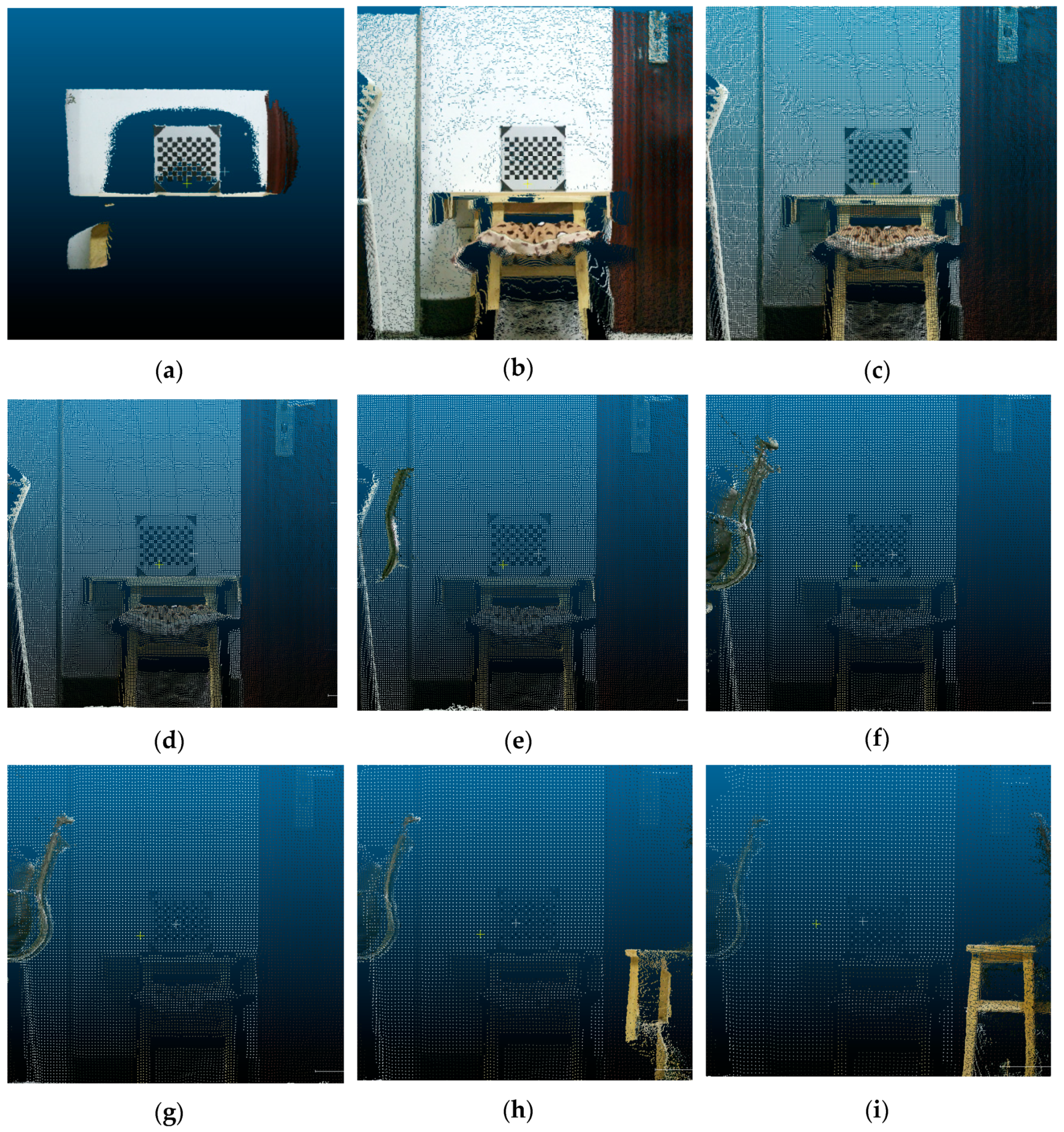
(2)

Checkerboard verification experiment: The checkerboard images were taken by the Kinect V2 camera every 500 mm from 500 to 5000 mm. Then, the coordinates of checkerboard corner points were extracted and compensated through the optimal compensation model separately. Finally, the RMSE of the checkerboard before and after RGB-D calibration was calculated and compared to verify the effect of the 3D compensation model.

(3)

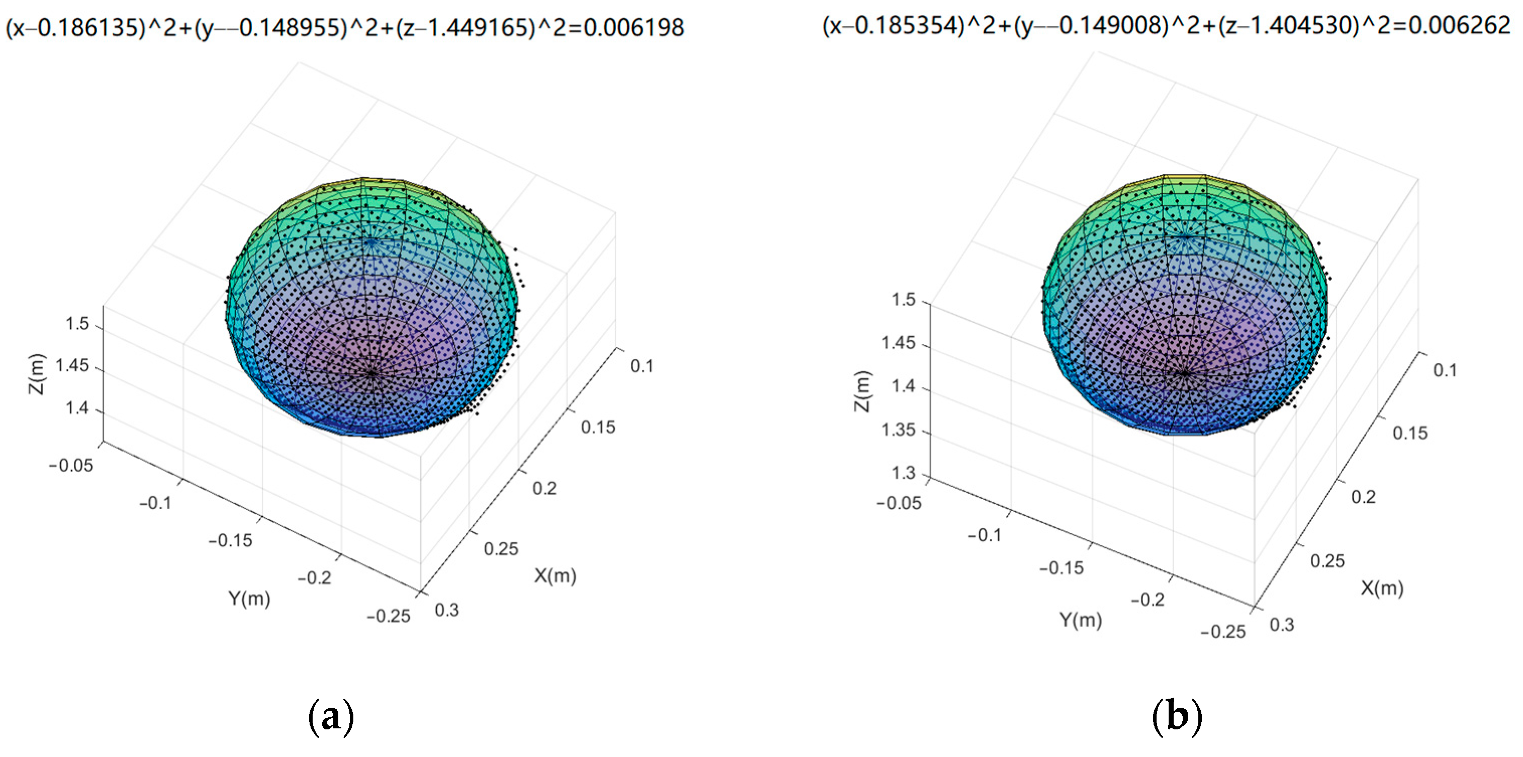
Sphere fitting experiment: The optimal model is applied to compensate for the spherical point cloud data captured by the Kinect V2 depth camera. Then, the original and compensated point cloud data are respectively substituted into the sphere fitting equation in Formula (14) to obtain the sphere parameters and residuals. Finally, the residual standard deviation is used to verify the effect of 3D compensation and reconstruction.

$$F(a,b,c,R)={(X_{\mathrm{sphere}}-a)}^2+{(Y_{\mathrm{sphere}}-b)}^2+{(Z_{\mathrm{sphere}}-c)}^2-R^2$$

(14)

where (X_sphere, Y_sphere, Z_Sphere) represents the 3D coordinates of the sphere; (a, b, c) are the coordinates of the center of the sphere and R is the radius of the sphere.

3. Results

The experimental design is as follows. The first step is to preprocess the 3D data, including eliminating the gross errors based on the BaySAC algorithm to obtain accurate inliers, computing the residual, and splitting all inliers into control points and check points. In the second step, three models for systematic error compensation are established based on control points, the cross validations are evaluated by checkpoints, and then the models are compared so that the optimal model can be selected. Finally, the checkerboard and real sphere data are used to verify the effectiveness of the compensation of the optimal 3D model that can be applied to the field of 3D modeling.

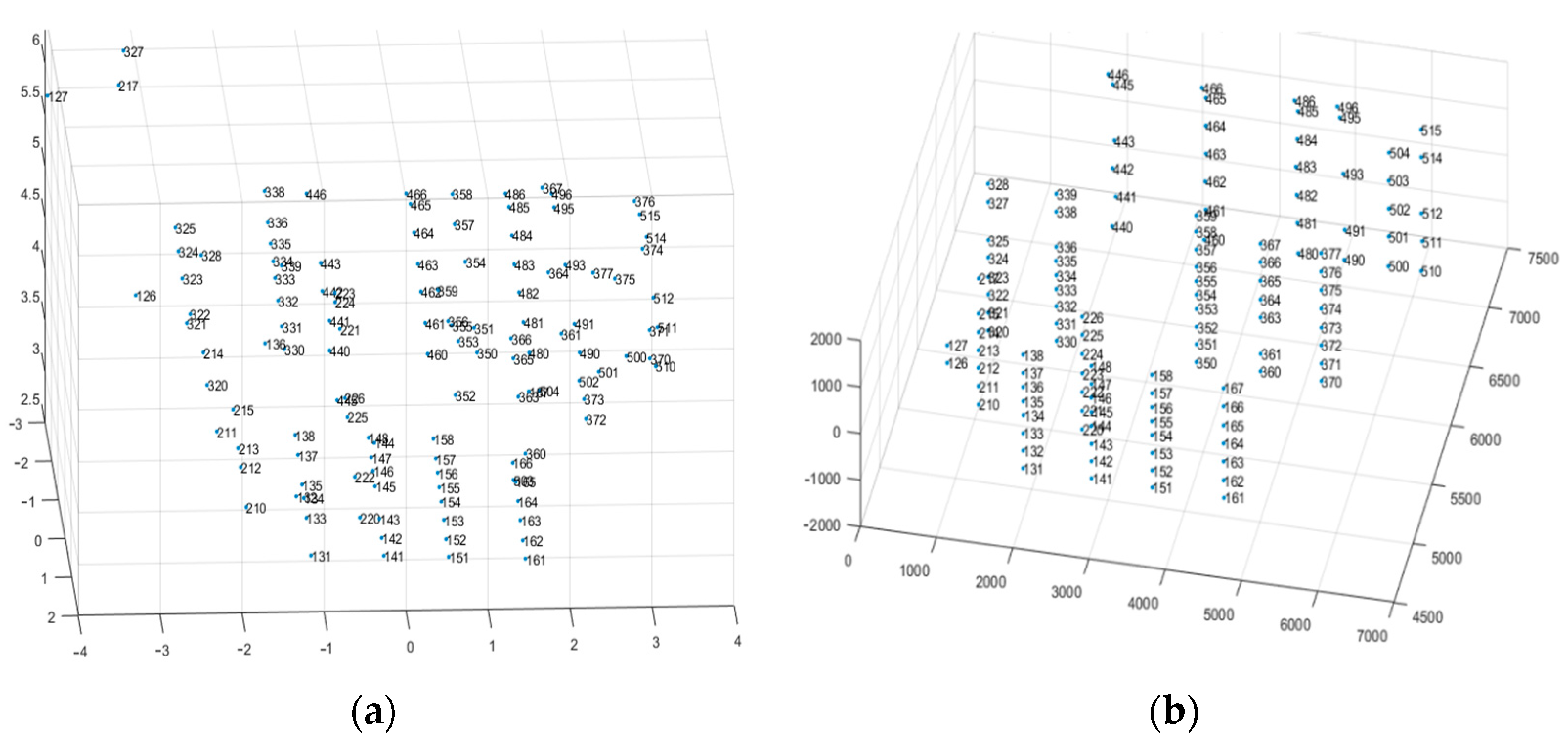
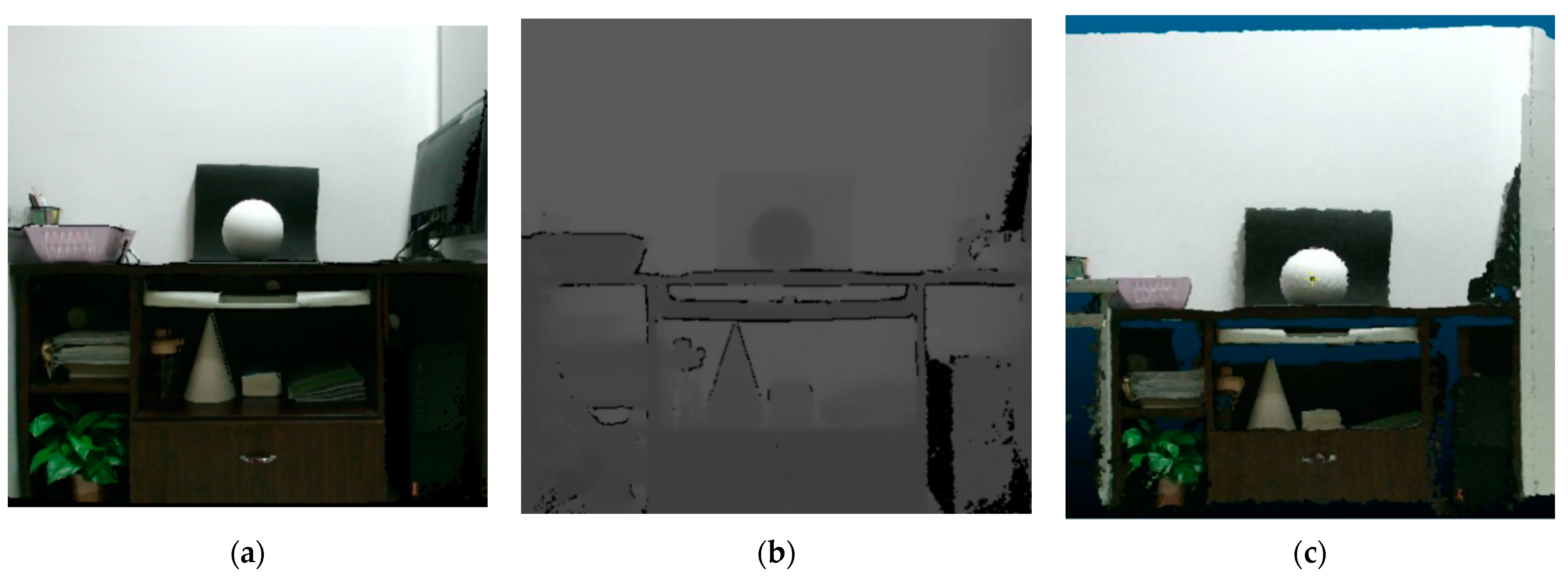
3.1. Pre-Processing of 3D Data

Figure 4a shows that even if there is considerable noise in the data, the outliers could be eliminated accurately by BaySAC. Then, the iteration method with variable weights was used to compute the parameters of the 3D registration model and control the slightly larger accidental errors in the data. The inliers were randomly and uniformly split into 80% control points and 20% check points 20 times, and one split of the dataset is shown in Figure 4b.

After the coordinate systems were unified, the residuals between the 3D coordinates of the corresponding points were calculated by Equation (9). Then, the results of the distribution and direction of the residual after coordinate transformation are shown in Figure 5, where the arrow represents the error vector. The figure shows that the error of Kinect V2 depth measurement is obviously related to the 3D coordinates of the measured object in space, and this verifies the systematic spatial distribution of the errors.

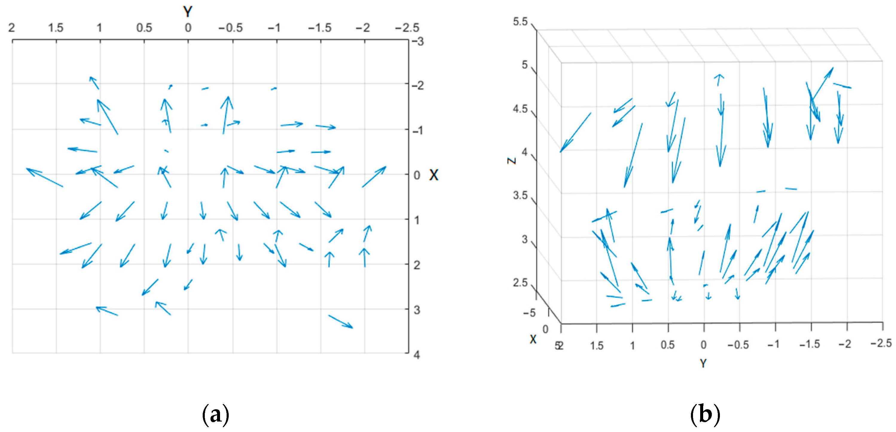
3.2. Establishment of Error Compensation Model in 3D Calibration Field

After the x and y errors of the 2D image were compensated by Formula (10), the errors in the depth direction were also compensated and calculated by stepwise regression, which can test the hypothesis and screen the parameters. Therefore, the optimal linear, quadratic, and cubic models for residual compensation are as follows:

Linear model:

$$\Delta d=a_0+a_1{x}^{\prime }+a_2{y}^{\prime }+a_4{r}^{\prime }$$

(15)

Quadratic model:

$$\Delta d=a_0+a_1{x}^{\prime }+a_2{y}^{\prime }+a_4{r}^{\prime }+a_9{x}^{\prime }{y}^{\prime }$$

(16)

Cubic model:

$$\Delta d=a_0+a_1{x}^{\prime }+a_2{y}^{\prime }+a_4{r}^{\prime }+a_9{x}^{\prime }{y}^{\prime }+a_{11}{x}^{\prime }{r}^{\prime }+a_{15}{x^{\prime }}^3+a_{25}{d}^2{x}^{\prime }+a_{31}{x}^{\prime }{y}^{\prime }d$$

(17)

Then, check points (i.e., cross validation) were substituted into the three models to calculate the RMSE and the percentage reduction of the error before and after correction in the 2D, depth and 3D directions. The average RMSEs of the 20% splits before and after correction were calculated. The results are shown in

Table 1. Effects of three error compensation models. Bolded numbers indicate the best accuracy in the comparison.

Dimension	Compensation Model	RMSE
		Before Correction	After Correction	Percentage Reduction of Error
2D	2D correction model	0.0963	0.0794	17.55%
Depth	Linear model	0.1828	0.0161	91.19%
	Quadratic model		0.0165	90.97%
	Cubic model		0.0174	90.48%
3D	Linear model	0.2066	0.0794	61.58%
	Quadratic model		0.0795	61.53%
	Cubic model		0.0797	61.45%

.

The result shows that all the 3D error compensation models can compensate for the systematic error to a certain extent. Compared with the quadratic and cubic models, the linear model is the most effective because it can compensate 91.19% of the error in the depth direction, and its coordinate error in the 3D direction can be reduced by 61.58% due to different denominators of percentages. Please note that the percentages of improvement calculated in the paper were acquired from the raw results of RMSE, but for presentation purposes, the results of before and after correction are rounded in the table, while the latter are referenced to this standard. The effect of the 3D compensation model outperforms that of the 2D and 1D (depth) compensation models. In addition, the r with better significance is retained.

3.3. Accuracy Evaluation Based on Checkerboard

To prove the generalization of the optimal compensation model for different distances, a high accuracy chessboard was used in the experiment. The data were taken by the Kinect V2 camera every 500 mm to acquire 10 sets of images, i.e., color images and corresponding depth images within the range of 500–5000 mm. As seen in Figure 6, many data points are missing due to the short distance at 500 mm.

Then, the coordinates of the checkerboard corner points at different distances were extracted and compensated through the optimal compensation model. The RMSEs before and after correction in the 3D direction are summarized in

Table 2. Compensation effect of the optimal model on the checkerboard at different distances.

Distance (mm)	RMSE
	Before Correction	After Correction	Percentage Reduction of Error
500	0.0463	0.0444	4.20%
1000	0.0694	0.0407	41.31%
1500	0.0846	0.0283	66.50%
2000	0.1268	0.0411	67.53%
2500	0.1374	0.0242	82.37%
3000	0.1611	0.0197	87.79%
3500	0.1958	0.0248	87.35%
4000	0.2200	0.0216	90.19%
4500	0.2889	0.0599	79.25%
5000	0.2092	0.0469	77.59%

.

The results show that all the error values of the data at different distances were improved. Although the compensation accuracies at distances of 500 mm (4.20%) and 1000 mm (41.31%) were relatively low, the compensation accuracy reached 60% at other distances, especially up to 90.19% at 4000 mm. The compensation effect increased to the maximum value at 4000 mm and then decreased at 4500 mm with the change in distance.

3.4. Accuracy Evaluation of the Model for Real Sphere Fitting

A regular gypsum sphere with a polished surface was used in this experiment. The Kinect V2 camera was utilized to collect color images at multiple angles, as shown in Figure 7a; and depth images, as shown in Figure 7b. The 3D point cloud data obtained after processing are shown in Figure 7c.

After the outliers were removed, the optimal 3D compensation model proposed was utilized to correct the spherical coordinates. Finally, the original coordinates and optimized coordinates were substituted into the sphere fitting model to calculate the sphere parameters and residual standard deviation, respectively.

In the results, the residual standard deviation of the coordinates before correction was 0.3354 mm and after correction was 0.3024 mm, and the error was reduced by 9.84%. The coordinates of the three directions can all be improved, and the sphere radius fit by the optimized coordinates was closer to the real value (shown in Figure 8b).

4. Discussion

We analyze and discuss the results of the above experiments as follows:

(1)

The optimized BaySAC algorithm can effectively eliminate gross errors. This occurs because the algorithm adds the influence of Bayesian prior probability into the RANSAC algorithm, which could reduce the number of iterations by half. In addition, a novel robust and efficient estimation method is applied that leads to the outliers being eliminated more accurately, and the relatively accurate coordinate transformation relationship can also be determined.

(2)

The accidental error could be further reduced by the iteration method with variable weights. In the parameter calculation process of the 3D registration model, the residuals between the matching points are used to update the weights until the iteration termination condition is reached. While more optimized parameters of the 3D registration model are obtained, the influence of larger accidental errors could also be reduced.

(3)

The systematic error of the depth camera could be controlled better by the error compensation model. Because some errors existed in the three directions of the depth data, compared with the 2D calibration field, the 3D calibration field with depth variation among control points can preferably meet the requirements of RGB-D camera calibration in the depth direction. Moreover, it is also helpful to obtain depth data with better accuracy.

(4)

Model optimization can reduce part of the model error. Three systematic error compensation models are established in the paper, and then we compared their compensation effects and selected the optimal model to calibrate the RGB-D camera. The results show that the linear model obtains the best compensation result. This may be because the essential errors of the Kinect V2 are relatively simple so that the linear model fits it well and has no overparameterization issue. Hence, the linear model has good generalization ability with simple parameters, while the quadratic and cubic models are relatively complicated.

(5)

The proposed compensation models are effective and have good generalization ability, which allows them to be applied to 3D modeling. This has been proven by the realization of the checkerboard and sphere fitting experiments, and the generalization differences are discussed below.

The checkerboard results show that the model has a good compensation effect in the appropriate shooting range (500–4500 mm) of the Kinect V2. However, the compensation effect gradually decreases when the distance is too close or too far. The result is consistent with that of the 3D calibration field, and some compensation effects are higher than the calibration field as the distance changes. The reason may be that the checkerboard has high manufacturing accuracy (±0.01 mm), and its surface has been specially treated by diffuse reflection and no light reflection so that the error caused by reflection is greatly reduced, which ensures original data quality.

In addition, the manufacturing process of the sphere may not be sufficiently strict; and the surface of the sphere is relatively smooth, which may result in some reflection errors. Hence, the compensation result is not as good as the 3D calibration field data and checkerboard.

5. Conclusions

In this paper, a Kinect V2 depth camera is taken as the research object and a new 3D compensation method for systematic error is proposed. The proposed linear model can better compensate for the systematic errors of a depth camera. The method considers overparameterization and provides a high-quality data source for 3D reconstruction.

Future work will focus on the depth measurement error caused by mixed pixels generated by low resolution and an estimation of the continuous depth value through the neighborhood correlation method. In addition, there are some more accurate camera calibration models (e.g., Sturm’s model [25]) that will be studied to further improve the 3D compensation accuracy for a Kinect RGB-D camera.

References

1. Lachat, E.; Macher, H.; Mittet, M.-A.; Landes, T.; Grussenmeyer, P. First Experiences with Kinect V2 Sensor For Close Range 3d Modelling. ISPRS-Int. Arch. Photogramm. Remote Sens. Spat. Inf. Sci. 2015, XL-5/W4, 93–100. [Google Scholar] [CrossRef] [Green Version]
2. Naeemabadi, M.; Dinesen, B.; Andersen, O.K.; Hansen, J. Investigating the impact of a motion capture system on Microsoft Kinect v2 recordings: A caution for using the technologies together. PLoS ONE 2018, 13, e0204052. [Google Scholar] [CrossRef] [PubMed]
3. Chi, C.; Bisheng, Y.; Shuang, S.; Mao, T.; Jianping, L.; Wenxia, D.; Lina, F. Calibrate Multiple Consumer RGB-D Cameras for Low-Cost and Efficient 3D Indoor Mapping. Remote Sens. 2018, 10, 328. [Google Scholar]
4. Choe, G.; Park, J.; Tai, Y.-W.; Kweon, I.S. Refining Geometry from Depth Sensors using IR Shading Images. Int. J. Comput. Vis. 2017, 122, 1–16. [Google Scholar] [CrossRef]
5. Weber, T.; Hänsch, R.; Hellwich, O. Automatic registration of unordered point clouds acquired by Kinect sensors using an overlap heuristic. ISPRS J. Photogramm. Remote Sens. 2015, 102, 96–109. [Google Scholar] [CrossRef]
6. Nir, O.; Parmet, Y.; Werner, D.; Adin, G.; Halachmi, I. 3D Computer-vision system for automatically estimating heifer height and body mass. Biosyst. Eng. 2018, 173, 4–10. [Google Scholar] [CrossRef]
7. Silverstein, E.; Snyder, M. Implementation of facial recognition with Microsoft Kinect v2 sensor for patient verification. Med. Phys. 2017, 44, 2391–2399. [Google Scholar] [CrossRef]
8. Guffanti, D.; Brunete, A.; Hernando, M.; Rueda, J.; Cabello, E.N. The Accuracy of the Microsoft Kinect V2 Sensor for Human Gait Analysis. A Different Approach for Comparison with the Ground Truth. Sensors 2020, 20, 4405. [Google Scholar] [CrossRef]
9. Cui, J.; Zhang, J.; Sun, G.; Zheng, B. Extraction and Research of Crop Feature Points Based on Computer Vision. Sensors 2019, 19, 2553. [Google Scholar] [CrossRef] [Green Version]
10. Wang, L.; Huynh, D.Q.; Koniusz, P. A Comparative Review of Recent Kinect-Based Action Recognition Algorithms. IEEE Trans. Image Process. 2020, 29, 15–28. [Google Scholar] [CrossRef] [Green Version]
11. Fankhauser, P.; Bloesch, M.; Rodriguez, D.; Kaestner, R.; Siegwart, R. Kinect v2 for Mobile Robot Navigation: Evaluation and Modeling. In Proceedings of the International Conference on Advanced Robotics (ICAR), Istanbul, Turkey, 27–31 July 2015. [Google Scholar]
12. Nascimento, H.; Mujica, M.; Benoussaad, M. Collision Avoidance Interaction Between Human and a Hidden Robot Based on Kinect and Robot Data Fusion. IEEE Robot. Autom. Lett. 2020, 6, 88–94. [Google Scholar] [CrossRef]
13. Wang, K.Z.; Lu, T.K.; Yang, Q.H.; Fu, X.H.; Lu, Z.H.; Wang, B.L.; Jiang, X. Three-Dimensional Reconstruction Method with Parameter Optimization for Point Cloud Based on Kinect v2. In Proceedings of the 2019 International Conference on Computer Science, Communications and Big Data, Bejing, China, 24 March 2019. [Google Scholar]
14. Lachat, E.; Landes, T.; Grussenmeyer, P. Combination of TLS point clouds and 3D data from Kinect V2 sensor to complete indoor models. ISPRS-Int. Arch. Photogramm. Remote Sens. Spat. Inf. Sci. 2016, XLI-B5, 659–666. [Google Scholar] [CrossRef] [Green Version]
15. Camplani, M.; Mantecón, T.; Salgado, L. Depth-Color Fusion Strategy for 3-D Scene Modeling With Kinect. IEEE Trans. Cybern. 2013, 43, 1560–1571. [Google Scholar] [CrossRef]
16. Maybank, S.J.; Faugeras, O.D. A theory of self-calibration of a moving camera. Int. J. Comput. Vis. 1992, 8, 123–151. [Google Scholar] [CrossRef]
17. Lachat, E.; Macher, H.; Landes, T.; Grussenmeyer, P. Assessment and Calibration of a RGB-D Camera (Kinect v2 Sensor) Towards a Potential Use for Close-Range 3D Modeling. Remote Sens. 2015, 7, 13070–13097. [Google Scholar] [CrossRef] [Green Version]
18. He, X.; Zhang, H.; Hur, N.; Kim, J.; Wu, Q.; Kim, T. Estimation of Internal and External Parameters for Camera Calibration Using 1D Pattern. In Proceedings of the IEEE International Conference on Video & Signal Based Surveillance, Sydney, Australia, 22–24 November 2006. [Google Scholar]
19. Koshak, W.J.; Stewart, M.F.; Christian, H.J.; Bergstrom, J.W.; Solakiewicz, R.J. Laboratory Calibration of the Optical Transient Detector and the Lightning Imaging Sensor. J. Atmos. Ocean. Technol. 2000, 17, 905–915. [Google Scholar] [CrossRef]
20. Sampsell, J.B.; Florence, J.M. Spatial Light Modulator Based Optical Calibration System. U.S. Patent 5,323,002A, 21 June 1994. [Google Scholar]
21. Hamid, N.F.A.; Ahmad, A.; Samad, A.M.; Ma’Arof, I.; Hashim, K.A. Accuracy assessment of calibrating high resolution digital camera. In Proceedings of the IEEE 9th International Colloquium on Signal Processing and its Applications, Kuala Lumpur, Malaysia, 8–10 March 2013. [Google Scholar]
22. Tsai, C.-Y.; Huang, C.-H. Indoor Scene Point Cloud Registration Algorithm Based on RGB-D Camera Calibration. Sensors 2017, 17, 1874. [Google Scholar] [CrossRef] [Green Version]
23. Wang, X.; Habert, S.; Ma, M.; Huang, C.H.; Fallavollita, P.; Navab, N. Precise 3D/2D calibration between a RGB-D sensor and a C-arm fluoroscope. Int. J. Comput. Assist. Radiol. Surg. 2016, 11, 1385–1395. [Google Scholar] [CrossRef]
24. Zhang, Z. A flexible new technique for camera calibration. IEEE Trans. Pattern Anal. Mach. Intell. 2000, 22, 1330–1334. [Google Scholar] [CrossRef] [Green Version]
25. Sturm, P.F.; Maybank, S.J. On plane-based camera calibration: A general algorithm, singularities, applications. In Proceedings of the IEEE Computer Society Conference on Computer Vision & Pattern Recognition, Fort Collins, CO, USA, 23–25 June 1999. [Google Scholar]
26. Boehm, J.; Pattinson, T. Accuracy of exterior orientation for a range camera. Int. Arch. Photogramm. Remote Sens. Spat. Inf. Sci. 2010, 38, 103–108. [Google Scholar]
27. Liu, W.; Fan, Y.; Zhong, Z.; Lei, T. A new method for calibrating depth and color camera pair based on Kinect. In Proceedings of the 2012 International Conference on Audio, Language and Image Processing (ICALIP), Shanghai, China, 16–18 July 2012. [Google Scholar]
28. Song, X.; Zheng, J.; Zhong, F.; Qin, X. Modeling deviations of rgb-d cameras for accurate depth map and color image registration. Multimed. Tools Appl. 2018, 77, 14951–14977. [Google Scholar] [CrossRef]
29. Gui, P.; Ye, Q.; Chen, H.; Zhang, T.; Yang, C. Accurately calibrate kinect sensor using indoor control field. In Proceedings of the 2014 3rd International Workshop on Earth Observation and Remote Sensing Applications (EORSA), Changsha, China, 11–14 June 2014. [Google Scholar]
30. Zhang, C.; Huang, T.; Zhao, Q. A New Model of RGB-D Camera Calibration Based On 3D Control Field. Sensors 2019, 19, 5082. [Google Scholar] [CrossRef] [PubMed] [Green Version]
31. Geiger, A.; Moosmann, F.; Car, O.; Schuster, B. Automatic camera and range sensor calibration using a single shot. In Proceedings of the 2012 IEEE International Conference on Robotics and Automation, Saint Paul, MN, USA, 14–18 May 2012; pp. 3936–3943. [Google Scholar]
32. Heikkila, J. Geometric camera calibration using circular control points. IEEE Trans. Pattern Anal. Mach. Intell. 2000, 22, 1066–1077. [Google Scholar] [CrossRef] [Green Version]
33. Kang, Z.; Jia, F.; Zhang, L. A Robust Image Matching Method based on Optimized BaySAC. Photogramm. Eng. Remote Sens. 2014, 80, 1041–1052. [Google Scholar] [CrossRef]
34. Fischler, M.A.; Bolles, R.C. Random Sample Consensus: A Paradigm for Model Fitting with Applications to Image Analysis and Automated Cartography. In Readings in Computer Vision; Fischler, M.A., Firschein, O., Eds.; Morgan Kaufmann: San Francisco, CA, USA, 1987; pp. 726–740. [Google Scholar]
35. Botterill, T.; Mills, S.; Green, R. New Conditional Sampling Strategies for Speeded-Up RANSAC. In Proceedings of the British Machine Vision Conference, BMVC, London, UK, 7–10 September 2009. [Google Scholar]
36. Li, D. Gross Error Location by means of the Iteration Method with variable Weights. J. Wuhan Tech. Univ. Surv. Mapp. 1984, 9, 46–68. [Google Scholar]
37. Brown, D.C. Close-range camera calibration. PE 1971, 37, 855–866. [Google Scholar]
Figure 1. The algorithm flowchart of 3D systematic error compensation for RGB-D cameras.
Remotesensing 13 04583 g001
Figure 2. Images collected from the 3D calibration field. (a) 3D calibration field; (b) RGB image within known calibration points; and (c) depth image.
Remotesensing 13 04583 g002
Figure 3. Coordinates of the control points in two coordinate systems. (a) In the depth camera; and (b) in the 3D calibration field.
Remotesensing 13 04583 g003
Figure 4. 3D points in RGB-D camera. (a) Inliers and outliers calculated by BaySAC; and (b) distribution of control points and check points.
Remotesensing 13 04583 g004
Figure 5. The error distribution and direction of observation points of the Kinect V2 RGB-D camera. (a) Error distribution under the XOY plane; and (b) error distribution in 3D space. The direction of the arrow indicates the direction of the error, and the unit in the figure is mm.
Remotesensing 13 04583 g005
Figure 6. Checkerboard data collected at different distances. (a) 500 mm; (b) 1000 mm; (c) 1500 mm; (d) 2000 mm; (e) 2500 mm; (f) 3000 mm; (g) 3500 mm; (h) 4000 mm; (i) 4500 mm; and (j) 5000 mm.
Remotesensing 13 04583 g006aRemotesensing 13 04583 g006b
Figure 7. Images of a sphere taken by a Kinect V2. (a) Color image; (b) depth image; and (c) 3D point cloud data.
Remotesensing 13 04583 g007
Figure 8. Compensation effect of optimal model on sphere data. (a) Before correction; and (b) After correction.
Remotesensing 13 04583 g008