Article

Exploring the Applicability and Scaling Effects of Satellite-Observed Spring and Autumn Phenology in Complex Terrain Regions Using Four Different Spatial Resolution Products

1
Key Laboratory of Regional Sustainable Development Modeling, Institute of Geographic Sciences and Natural Resources Research, Chinese Academy of Sciences, Beijing 100101, China
2
College of Resources and Environment, University of Chinese Academy of Sciences, Beijing 100049, China
3
State Key Laboratory of Remote Sensing Science, Aerospace Information Research Institute, Chinese Academy of Sciences, Beijing 100101, China
4
National Remote Sensing Center of China, Beijing 100036, China
*
Author to whom correspondence should be addressed.
Remote Sens. 2021, 13(22), 4582; https://doi.org/10.3390/rs13224582
Submission received: 24 September 2021 / Revised: 10 November 2021 / Accepted: 11 November 2021 / Published: 15 November 2021
(This article belongs to the Special Issue Remote Sensing of Land Surface Phenology)

Abstract

:
The information on land surface phenology (LSP) was extracted from remote sensing data in many studies. However, few studies have evaluated the impacts of satellite products with different spatial resolutions on LSP extraction over regions with a heterogeneous topography. To bridge this knowledge gap, this study took the Loess Plateau as an example region and employed four types of satellite data with different spatial resolutions (250, 500, and 1000 m MODIS NDVI during the period 2001–2020 and ~10 km GIMMS3g during the period 1982–2015) to investigate the LSP changes that took place. We used the correlation coefficient (r) and root mean square error (RMSE) to evaluate the performances of various satellite products and further analyzed the applicability of the four satellite products. Our results showed that the MODIS-based start of the growing season (SOS) and end of the growing season (EOS) were highly correlated with the ground-observed data with r values of 0.82 and 0.79, respectively (p < 0.01), while the GIMMS3g-based phenology signal performed badly (r < 0.50 and p > 0.05). Spatially, the LSP that was derived from the MODIS products produced more reasonable spatial distributions. The inter-annual averaged MODIS SOS and EOS presented overall advanced and delayed trends during the period 2001–2020, respectively. More than two-thirds of the SOS advances and EOS delays occurred in grasslands, which determined the overall phenological changes across the entire Loess Plateau. However, both inter-annual trends of SOS and EOS derived from the GIMMS3g data were opposite to those seen in the MODIS results. There were no significant differences among the three MODIS datasets (250, 500, and 1000 m) with regard to a bias lower than 2 days, RMSE lower than 1 day, and correlation coefficient greater than 0.95 (p < 0.01). Furthermore, it was found that the phenology that was derived from the data with a 1000 m spatial resolution in the heterogeneous topography regions was feasible. Yet, in forest ecosystems and areas with an accumulated temperature ≥10 °C, the differences in phenological phase between the MODIS products could be amplified.

1. Introduction

Land surface phenology (LSP) has been recognized as one of the most effective indicators of climate change [1,2,3,4] and is closely related to animal migration, gross primary production, and crop productivity [5,6,7]. Methods for measuring phenology include ground observations (i.e., PhenoCam network and phenology network) and satellite observations [8,9,10]. Ground observations usually only reflect the phenological information of local ecological communities [11,12,13]. However, satellite remote sensing has the potential to continuously observe the variation in vegetation phenology at multiple scales [14,15,16,17].
Phenology has been widely monitored in different types of remote sensing data in attempts to understand the interactions between vegetation and climate change during the past few decades [18,19,20,21,22]. A variety of vegetation indexes were used to monitor vegetation phenology in previous studies [23,24,25]. The two most used vegetation indices are the enhanced vegetation index (EVI) and the normalized difference vegetation index (NDVI) [26,27,28,29]. Meanwhile, several sets of freely accessible remote sensing products with different resolutions were released, such as the third generation GIMMS (GIMMS3g) NDVI with a spatial resolution of 1/12 degree that is derived from the Advanced Very-High-Resolution Radiometer (AVHRR) series satellites [30,31]; the Systeme Probatoire d’Observation de la Tarre (SPOT) NDVI with a 1 km spatial resolution [32]; and the moderate-resolution imaging spectroradiometer (MODIS) NDVI with spatial resolutions of 250, 500, or 1000 m [33,34]. Among them, GIMMS3g NDVI is the latest and longest-used product, and MODIS NDVI has several different spatial resolutions. These products have been widely used for studies involving phenology extraction [15]. Recent studies showed that the temporal and spatial variation trends of vegetation phenology that were observed in some areas by GIMMS3g NDVI and MODIS NDVI were consistent, but the conclusions that were reached in other regions were opposite [35,36]. The topography has a significant impact on the phenology of different product identifications [37]. Furthermore, the spatial phenological heterogeneity of data with a different resolution increases with the increase in landscape fragmentation [5]. However, the impacts of satellite products with different spatial resolutions on LSP extraction over regions with a heterogeneous topography have not been well clarified.
In general, data with a finer spatial resolution possess more information about the seasonality and phenology properties of vegetation [38,39,40]. Meanwhile, data with a fine spatial resolution have the problem of providing a larger amount of data, having a slow computation speed, and being time-consuming [41]. The coarse spatial resolution data is more suitable for monitoring phenology at a landscape scale [42]. Moreover, there will be some differences in vegetation phenology that are estimated from the coarse spatial resolution data to the fine spatial resolution data [5]. Thus, it is important to select remote sensing products with an appropriate spatial resolution in order to investigate vegetation phenology changes.
In this study, we explored the applicability of 250, 500, and 1000 m MODIS NDVI and GIMMS3g NDVI across the entire Loess Plateau, which is a typically ecological fragile region with a heterogeneous topography. The aims of this study were to (1) investigate the spatial and temporal patterns of vegetation phenology in the Loess Plateau, (2) analyze the applicability of different types of satellite data in complex terrain regions, and (3) explore the factors that influence the differences in the phenology of multiple datasets.

2. Materials and Methods

2.1. Study Area

The Loess Plateau lies in the north of China, covering an area of 62.4 × 10⁴ km2 (Figure 1). The region is dominated by a continental monsoon climate. The annual accumulated temperature ≥10 °C (annual AT10) increases from ~50 °C·d in the high-elevation western part to ~5800 °C·d in the southern part. Additionally, the annual mean precipitation varies from 50 mm in the northwest to 700 mm in the southeast. The terrain of the Loess Plateau varies significantly, and the altitude ranges from 80 m in the southeast to 5200 m in the west. Land use data with a spatial resolution of 500 m from the MODIS land cover product (MCD12Q1) show that there are seven land cover types in the entire study area; these are grasslands (68.5%), croplands (21.2%), forests (5.1%), barren regions (3.3%), urban and built-up areas (1.8%), and water bodies (0.1%).

2.2. Data Resources and Preprocessing

In this study, we used four types of satellite data: MODIS NDVI with spatial resolutions of 250, 500, and 1000 m and GIMMS3g NDVI with a spatial resolution of ~10 km. These data have been widely applied for vegetation phenology extraction at regional to global scales [43,44,45]. MODIS data for the period 2001–2020 were acquired from NASA (ftp://ladsweb.nascom.nasa.gov/allData/6/, accessed on 15 April 2021). MODIS NDVI with a temporal resolution of 16 days is a gridded level 3 product. GIMMS3g NDVI was obtained from the NASA Earth Exchange platform for the period 1982–2015 (https://nex.nasa.gov/nex/, accessed on 15 April 2021). The spatial and temporal resolution of the GIMMS3g NDVI was 15 days and 1/12 degree (~10 km), respectively. Both the MODIS and GIMMS3g time-series datasets were used to identify the start of the growing season (SOS) and the end of the growing season (EOS).
The daily mean air temperature with a spatial resolution of 0.25 degrees for the period 1982–2020 was obtained from the Copernicus Climate Change Service Climate Data Store (CDS) (https://cds.climate.copernicus.eu/#!/home, accessed on 19 June 2021). The daily air temperature was used to obtain AT10 in order to analyze the interaction between phenology and temperature.
The annual MODIS land cover type product at a 500 m spatial resolution was used to examine the influence of vegetation type on the LSP. The classification scheme that is used for the product is the International Geosphere–Biosphere Program (IGBP). Additionally, the year used for the latest MODIS land cover type data was 2019. The land cover type product for the period 2001–2019 was obtained from NASA’s Land Processes Distributed Active Archive Center (LP DAAC) (https://lpdaac.usgs.gov/products/mcd12q1v006/, accessed on 19 June 2021). The spatial resolution of the product was resampled to 250 m, 1000 m, and 1/12 degree using nearest-neighbor interpolation. The Shuttle Radar Topography Mission (SRTM) digital elevation model (DEM) dataset was achieved at the CGIAR (https://srtm.csi.cgiar.org/, accessed on 11 July 2021). The DEM dataset was used to understand the distribution of the topography in the Loess Plateau. The terrain of the central and western parts of the Loess Plateau is heterogeneous, while the terrain of the Weihe Plain is flat [46].
The 271 detailed ground-observed records in the Loess Plateau were obtained from 14 agro-meteorological stations from 2001 to 2013 (a small set of data with low quality was rejected). The distributions and information of the ground-observed sites can be found in Figure 1a and Table 1. The observed records were used to validate the vegetation phenology that was derived from MODIS data and more information could be used as prior knowledge of the research area [47].

2.3. Methods

The quality of the NDVI time series was first examined based on the QA information. The LSP was not produced if three serial periods of NDVI data were contaminated by clouds. Second, to reduce the impacts of noise from cloud contamination or other poor atmospheric conditions, the MODIS NDVI time series were smoothed using the modified Savitsky–Golay algorithm (mSG) with the help of a specific MODIS data layer named “composite day of the year” [19,48]. Similarly, the GIMMS3g NDVI data were also smoothed. However, the GIMMS3g data lacked the layer of “composite day of the year”; we thus regarded the 1st and 16th days of each month as the “day of year (DOY)” for each image. The mSG algorithm is a simple but robust method that is based on the Savitsky–Golay algorithm [48,49]. Finally, the smoothed NDVI growth curve was used to estimate the SOS and EOS with the following logistic model [34]:
y ( t ) = c 1 + e a + b t + d ,
where t is the DOY, y(t) represents the NDVI value at time t, a and b are the fitting parameters, c is the difference between the maximum and minimum NDVI values, and d is the initial background vegetation index value. Next, the SOS and EOS were produced from the rate of change in curvature:
K = b 2 c z ( 1 z ) ( 1 + z ) 3 [ ( 1 + z ) 4 + ( b c z ) 2 ] 3 / 2
K = b 3 c z {   3 z ( 1 z ) ( 1 + z ) 3 [ 2 ( 1 + z ) 3 + b 2 c 2 z ] [ ( 1 + z ) 4 + ( b c z ) 2 ] 5 / 2 ( 1 + z ) 2 ( 1 + 2 z 5 z 2 ) [ ( 1 + z ) 4 + ( b c z ) 2 ] 3 2   }
where K represents the curvature, z = e a + b t , and K′ is the rate of change of K.
In order to acquire the deviation and the correlation characteristics between different products, the root mean square error (RMSE) and correlation coefficient (r) were calculated using Equations (4) and (5), respectively:
R M S E = i = 1 n ( X i X ¯ ) 2 n
where X ¯ is the mean value of X and ( X i X ¯ ) represents the deviation value, that is, the bias;
r = i = 1 n ( X i X ¯ ) ( Y i Y ¯ ) i = 1 n ( X i X ¯ ) 2 i = 1 n ( Y i Y ¯ ) 2
where X i and Y i correspond to two different datasets.
Based on the geographical location information of agro-meteorological stations, we first extracted the SOS and EOS pixels (e.g., 3 × 3 homogeneous pixels) around the center of each station, and then averaged these values to obtain the mean SOS and EOS of each station [50]. Finally, we employed RMSE and r to investigate the correlation between the satellite-based and ground-observed phenology.

3. Results

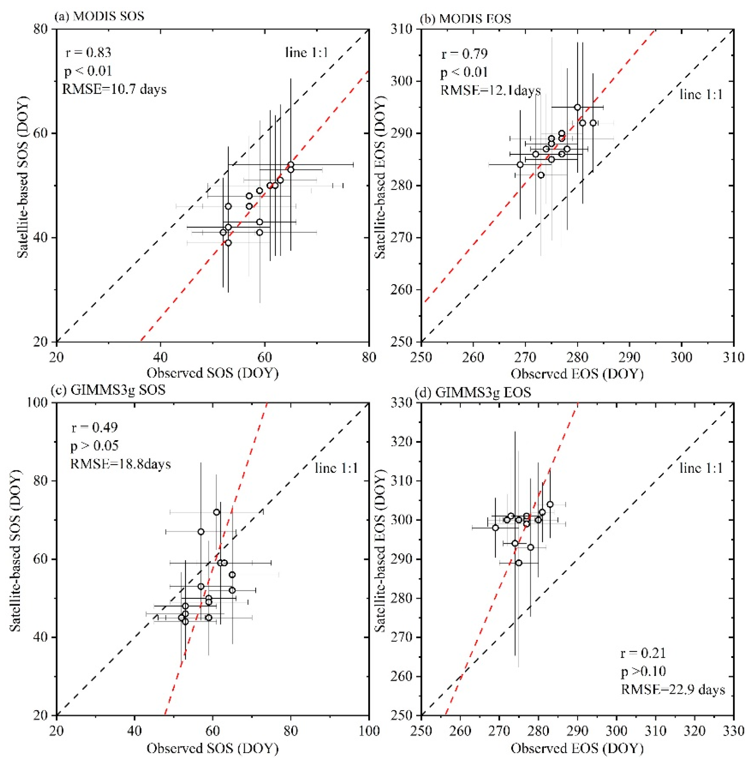
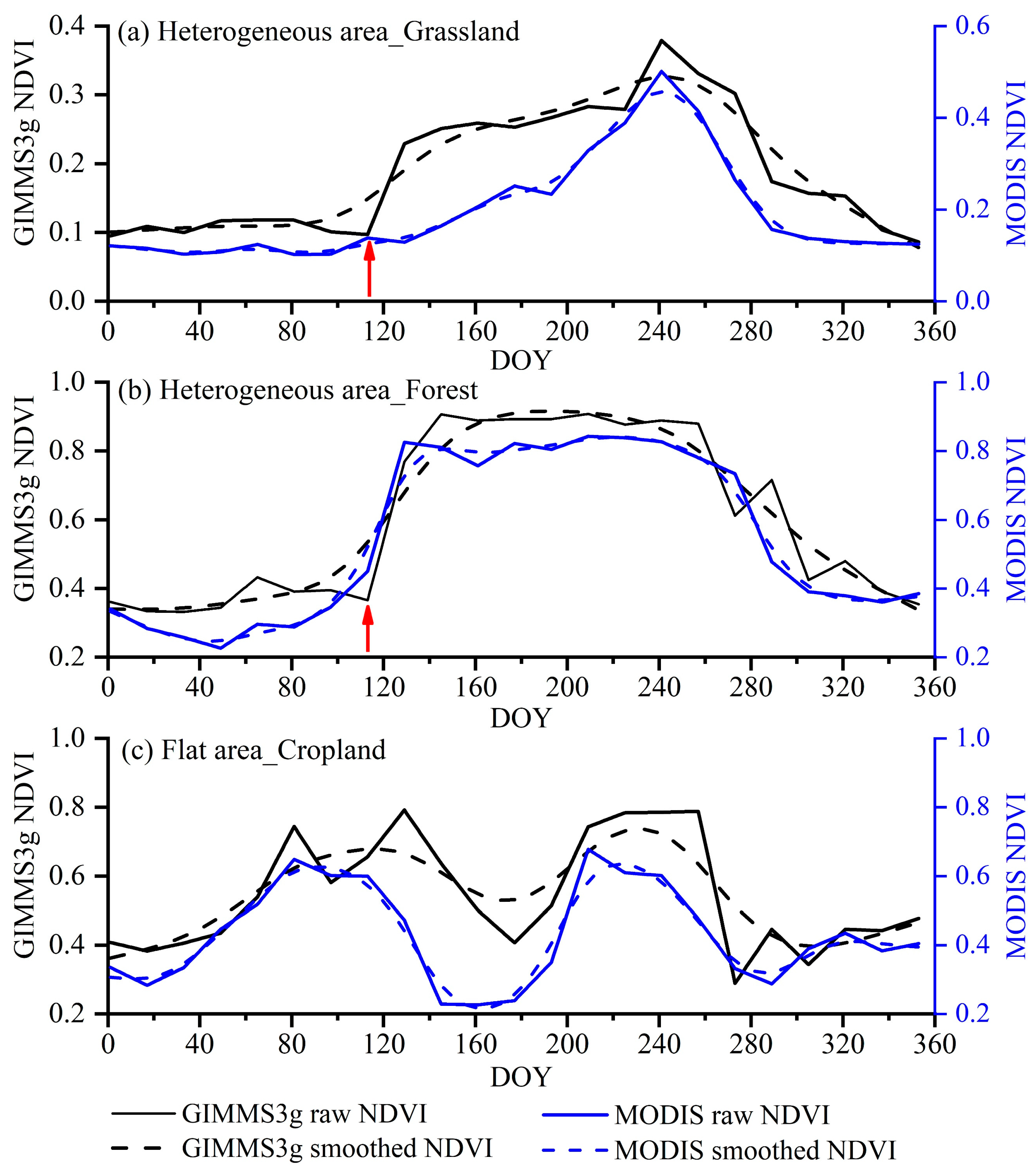
3.1. The Performances of Satellite-Based SOS and EOS

This study first verified the performances of the SOS and EOS that were produced from the 250 m MODIS NDVI and GIMMS3g NDVI against the ground-observed data from 2001 to 2013. The results showed that a good agreement was observed between the MODIS-derived phenology and ground-observed data, where the r values of the MODIS SOS and EOS were 0.83 and 0.79, respectively (p < 0.01, Figure 2). However, the phenology that was estimated from GIMMS3g NDVI showed poor consistency. The r values of the GIMMS3g SOS and EOS were only 0.49 and 0.21, and both the p-values were more than 0.05.

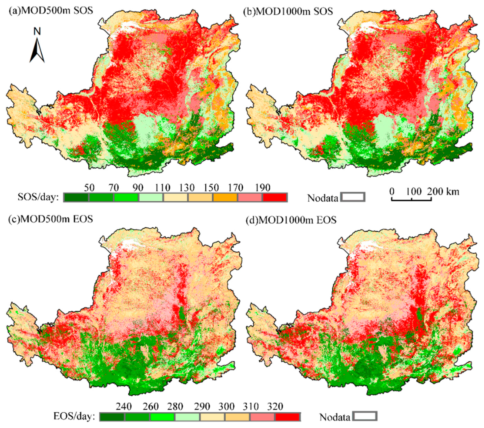
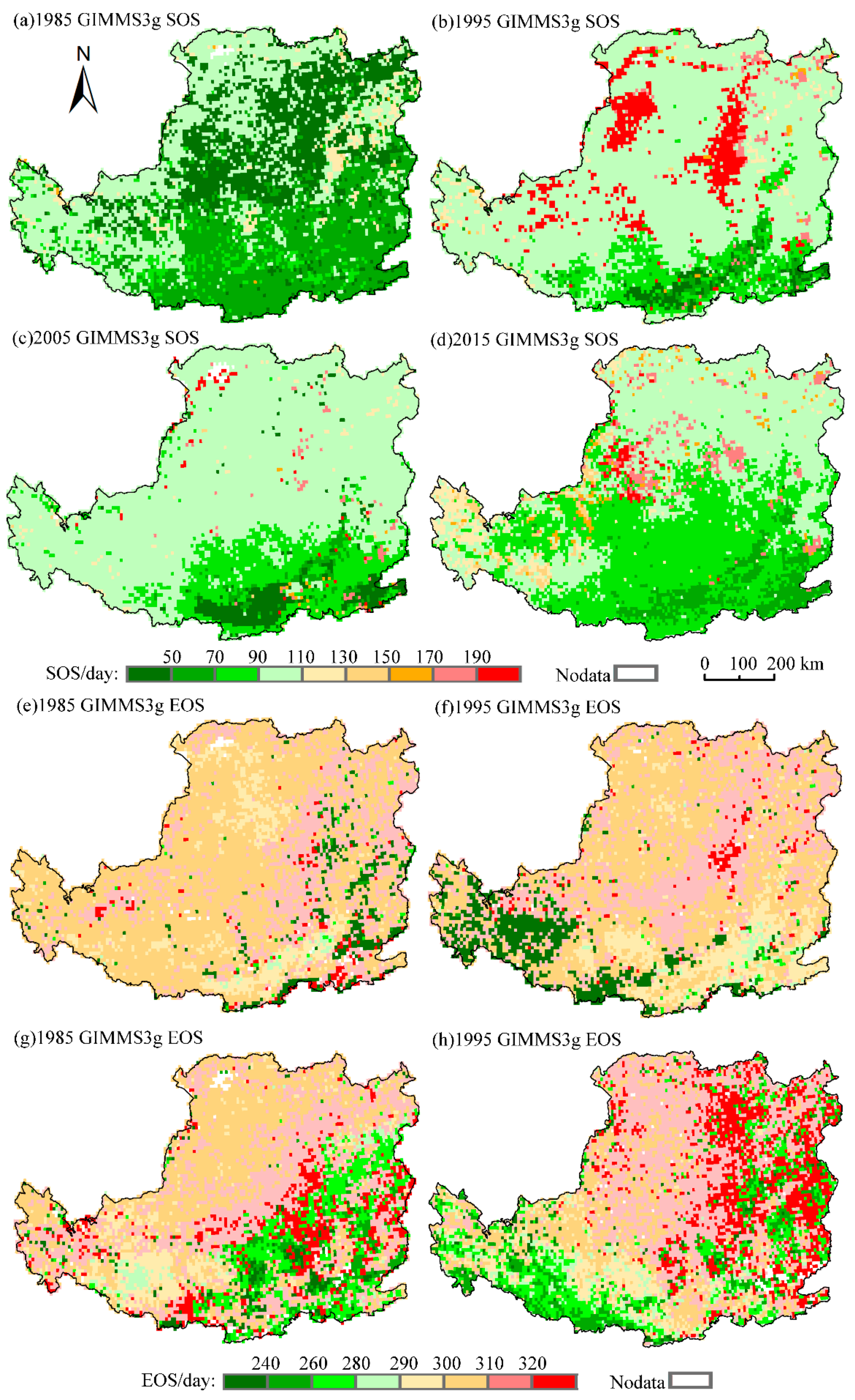
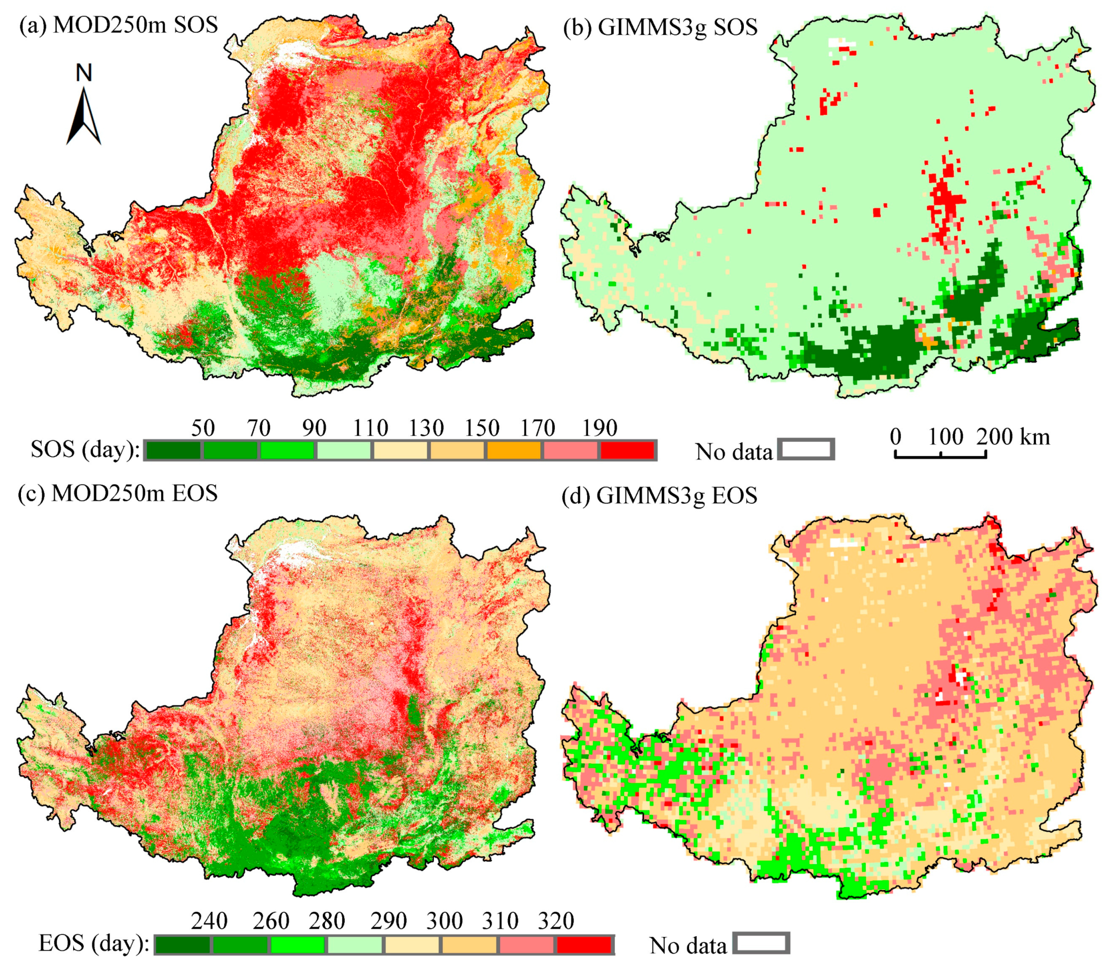
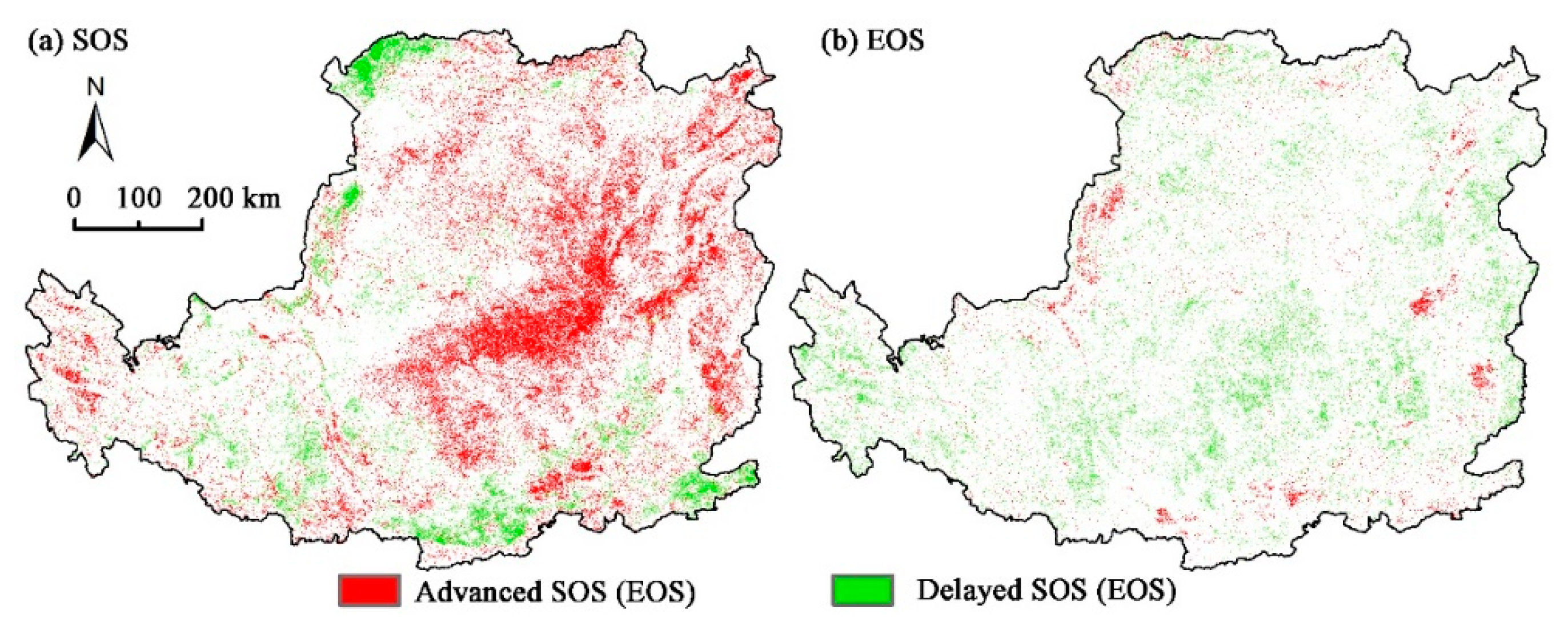
3.2. Spatial Patterns of Vegetation Phenology

Figure 3 presents the SOS and EOS of the Loess Plateau in 2001. The spatial patterns of the vegetation phenology that were produced from the GIMMS3g data were quite different from those of the MODIS data. However, three sets of MODIS phenology results with different resolutions gave a similar spatial distribution (Figure A1). The spring phenology of croplands in the Weihe Plain was the earliest, with an average SOS of DOY 46. Most SOSs in the grassland region of the central Loess Plateau were later than DOY 170. In particular, the SOS that was derived from MODIS NDVI in the Mu Us Sandy Land region was earlier than that in the surrounding areas. The early EOS in the Loess Plateau was mainly concentrated in the southern region, while the late EOS was mainly concentrated in the western region and the Lvliang mountains. Among the land cover types, the EOS of almost 80% of the croplands was between DOY 260 and 290, the EOS date of the forests was the earliest, and that of the grasslands was the latest.
Compared with the MODIS-derived phenology, the spatial distribution of the phenology period that was identified by the GIMMS3g data was more concentrated. Moreover, the SOS values that were derived from the GIMMS3g product were largely consistent with the phenology that was derived from the MODIS data, which was mainly distributed in the Weihe Plain. The SOS that was produced by the GIMMS3g NDVI data in the northern part of the Loess Plateau was concentrated in DOY 90–110, and the spatial details were greatly neglected. Additionally, there was a significant difference between the GIMMS3g EOS and the MODIS EOS in the south–central region of the Loess Plateau. The difference ranged from 20 days to more than 60 days.
Figure 4a,b presents the raw and smoothed NDVI in heterogeneous areas, where the land use types are grassland and forest, respectively. Figure 4c shows that the time series of NDVI in the Weihe Plain, where the land use type was cropland. Based on the time-series data, we found that no matter what year it was, the inflection point of the time series of the original GIMMS3g data was always concentrated in the seventh or eighth period’s data in heterogeneous areas. However, this phenomenon did not occur in flat areas. This indicates that the problem of GIMMS3g data is one of the important reasons for the spatially aggregated distribution of GIMMS3g phenology.
In order to compare the differences between the GIMMS3g-derived and MODIS-derived phenology in flat areas, we calculated the differences of the two datasets in the Weihe Plain during the period 2001–2015 (Figure 5). The findings showed that the differences in SOS (GIMMS3g SOS–250 m MODIS SOS) were mainly less than 5 days and 10 days in 43.49% and 70.66%. The GIMMS3g data performed well at monitoring SOS over the flat areas. In addition, we found that the frequency with which the differences in SOS were greater than 20 days decreased significantly and became close to 0. In the results showing the SOS differences greater than 25 days, the value of the GIMMS3g SOS was always greater than that of the 250 m MODIS SOS. This shows that GIMMS3g SOS tended to be later than MODIS SOS. However, differences in the EOS (GIMMS3g EOS–250 m MODIS EOS) that were less than 5 days or 10 days were only 13.85% and 29.88%. In addition, for the entire Loess Plateau, the proportion of differences in EOS between the GIMMS3g and 250 m MODIS data that were less than 5 days was still less than 20%. This indicated that the consistency of the GIMMS3g EOS and the MODIS EOS was poor, even in flat areas.

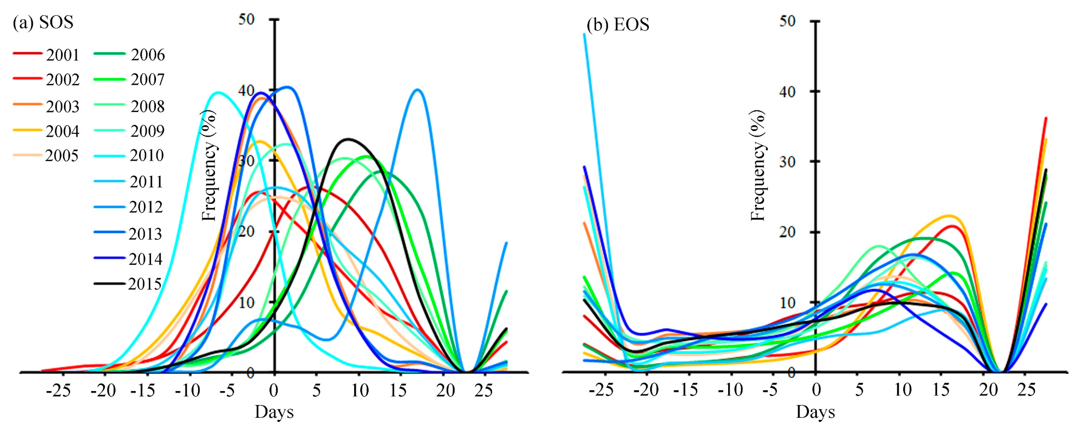
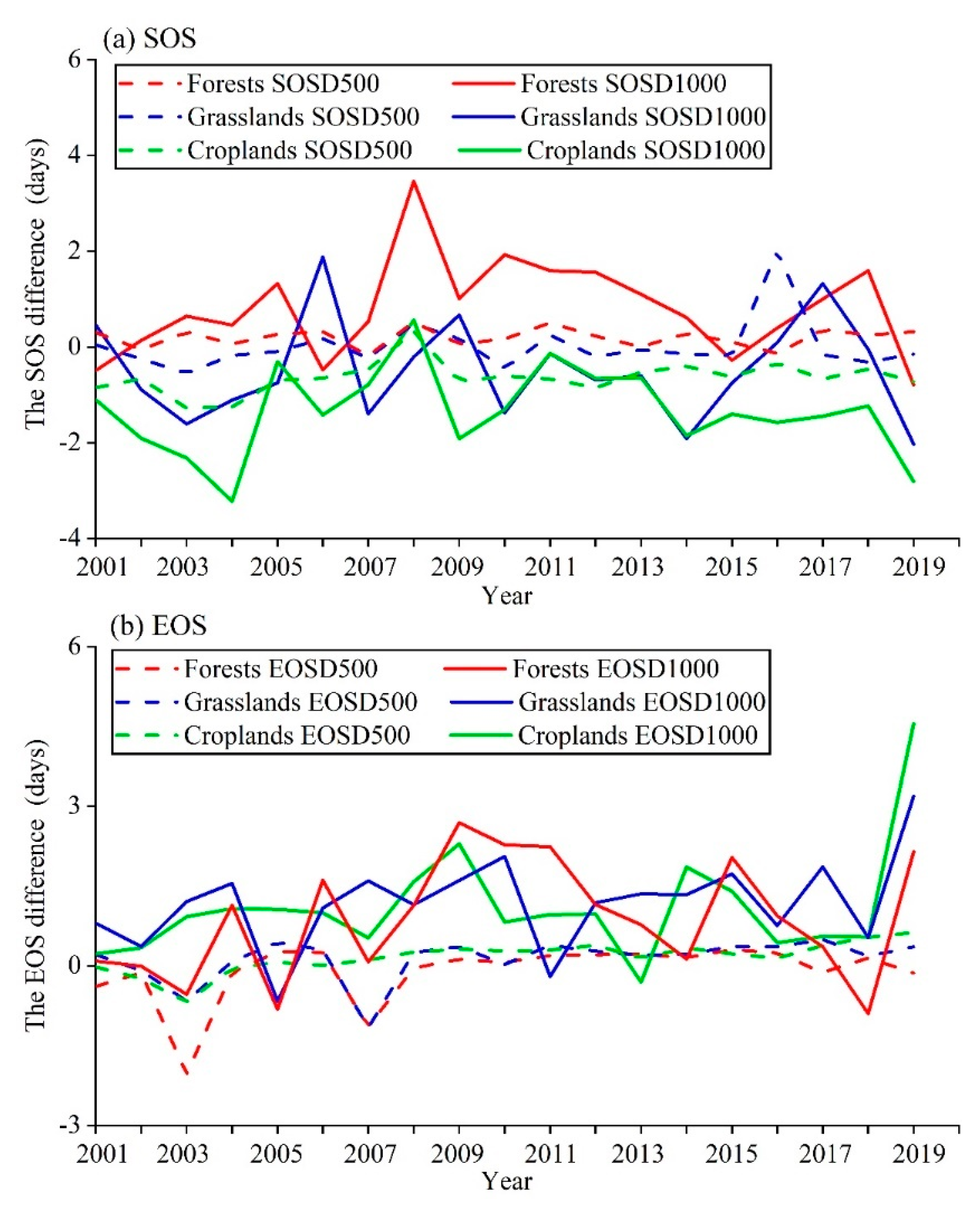
3.3. Temporal Variation in Vegetation Phenology

The inter-annual trends of the SOS and EOS during the period 1982–2020 are presented in Figure 6. The results showed that the inter-annual trends of the SOS and EOS from GIMMS3g were the reverse of those of the MODIS data. The SOS showed a trend of postponing and the EOS presented a trend of advancing from 1982 to 2015 based on the GIMMS3g data. In addition, the SOS (EOS) of the GIMMS3g data delay (advance) trend during the period 2001–2015 was more significant, and the trend lines K of the SOS and EOS were 0.34 and −0.14, respectively. In contrast, the SOS (EOS) showed an advanced (delayed) trend based on the MODIS data, and the trend line K of the MODIS SOS and EOS was −0.63 and 0.19, respectively, during the period 2001–2015.
In the comparison of MODIS products, our findings showed that the phenological periods that were derived from MODIS products with various spatial resolutions gave only small differences. The average difference between the 500 m MODIS SOS (EOS) and 250 m MODIS SOS (EOS) was only 1.2 (0.3) days. The correlation coefficient and RMSE between the 500 m MODIS and 250 m MODIS results were greater than 0.99 and less than 0.60, respectively (Table 2). Moreover, the average difference between the 1000 m MODIS SOS (EOS) and 250 m MODIS slightly increased to 1.7 (1.4) days. The correlation coefficient and RMSE between the 1000 m MODIS and 250 m MODIS results were greater than 0.95 and approximately equal to 1.0, respectively. This demonstrated that there was little difference between the 1000 m MODIS NDVI and the 250 m MODIS NDVI. Therefore, the 1000 m MODIS NDVI could be used to monitor the LSP of the Loess Plateau. However, the GIMMS3g product may not be able to accurately monitor heterogeneous areas, such as the Loess Plateau.
Figure 7 shows the spatial trend of the phenology over the Loess Plateau that was calculated from the MODIS data during the period 2001–2020, which passed the significance test of α = 0.05. The area with a significantly advanced SOS was about 16.7 × 10⁴ km2, which was about a quarter of the area of the Loess Plateau. Areas with a significantly advanced SOS were mainly in the central and northeastern regions of the Loess Plateau. The area of the delayed SOS was only one-third that of the advanced SOS. Meanwhile, the delayed SOS was mainly distributed across the croplands of the Weihe and Hetao Plains. Moreover, the area with a significantly delayed EOS was about 9.3 × 10⁴ km2, which was more than three times that of the area with an advanced EOS. More than two-thirds of the advanced SOS and delayed EOS occurred in grasslands, which determined the overall phenological changes in the Loess Plateau. Although the land cover types in the Loess Plateau changed dramatically, the phenological changes were still dominated by the areas where the land use did not change. Only about 20% of the SOS or EOS significant trends occurred in areas with changes in the land cover type.

3.4. Impact Factors on MODIS Products

3.4.1. Influences of Vegetation on MODIS Products

To examine the possible causes of the difference in LSP from the MODIS data, we investigated the differences in the SOSs and EOSs between MODIS products that were used on different land cover types (Figure 8). Our findings showed that the largest difference between the 250 m MODIS SOS and the 1000 m MODIS SOS (1000 m MODIS SOS–250 m MODIS SOS) in forests was 3.5 days, which was larger than the difference found in grasslands (1.9 days) and croplands (0.6 days). Additionally, the standard deviation of the inter-annual difference between the 250 m and 1000 m MODIS SOS in forests was 1.1 days, which was the largest value that was obtained among all vegetation types. The differences that were obtained between the 250 m MODIS EOS and the 1000 m MODIS EOS were 0.9 days (forests), 1.2 days (grasslands), and 1.1 days (croplands). The standard deviation of the inter-annual difference was the largest in forests. In addition, we found that the differences in the SOS between the 250 m MODIS and 500 m MODIS (500 m MODIS SOS–250 m MODIS SOS) were both less than one day.

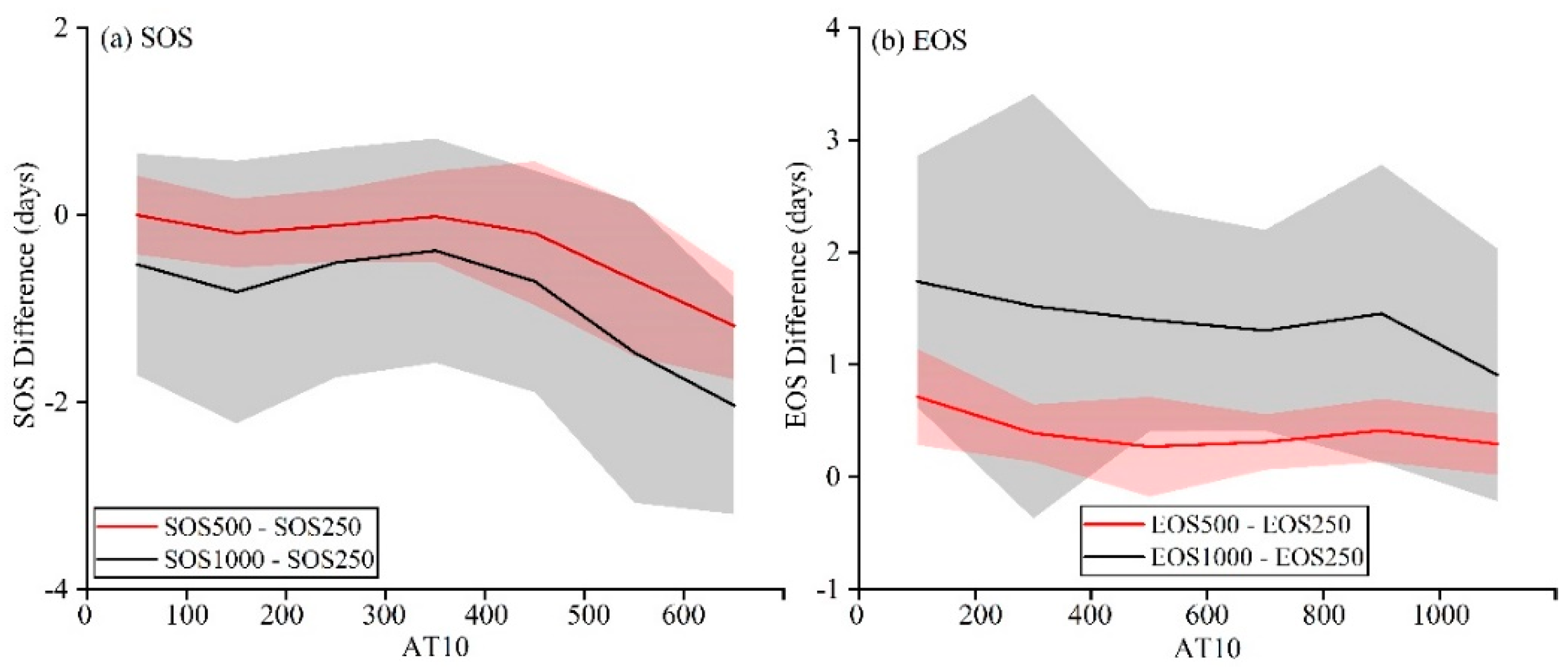
3.4.2. Influences of AT10 on the Phenology

Figure 9 presents the variations in the differences that were obtained between multiple sets of the SOS and EOS with an AT10 from 1 January to 30 April and from 1 September to 31 October, respectively. As the AT10 from January to April increased, the difference between each MODIS SOS gradually increased. In particular, the difference between the 1000 m MODIS SOS and the 250 m MODIS SOS (1000 m MODIS SOS–250 m MODIS SOS) was greater than the difference between the 500 m MODIS SOS and the 250 m MODIS SOS (500 m MODIS SOS–250 m MODIS SOS). The standard deviation of the 1000 m MODIS SOS was greater than that of the 500 m MODIS SOS. The relationship between the EOS and AT10 was found to be opposite to that of the SOS and AT10. Our results showed that with the increase in AT10 from September to October, the difference between each MODIS EOS gradually decreased. No matter whether the SOS or EOS were used, the difference in vegetation phenology between the 250 m and 1000 m products was less than 3 days. Additionally, we found that there was almost no difference between the 250 m and 500 m vegetation phenology.

4. Discussion

4.1. Difference between Satellite-Based LSP and Observations

Based on the MODIS NDVI and the layer named “composite day of the year,” we calculated three sets of MODIS phenology with different spatial resolutions from 2001 to 2020. The GIMMS3g data lacked a “composite day of the year” layer, therefore we regarded the 1st and 16th days of each month as the DOY and calculated the GIMMS3g phenology from 1982 to 2015. We used the ground-observed data during the period 2001–2013 to verify the performances of the phenology that was derived from the MODIS and GIMMS3g data. Our results showed that the MODIS-derived phenology and ground-observed data had a good agreement, but that the correlation between the GIMMS3g-derived phenology and ground-observed data was very bad. This indicates that the SOS and EOS that were identified by the MODIS NDVI were more robust, but that the GIMMS3g phenology performed badly.
Moreover, the MODIS SOS that was identified by the logistics model was earlier than the SOS that was observed on the ground, while the MODIS EOS was later than the ground-observed data. Similarly, previous studies also found that in the north of China, the SOS that was identified by the logistics model based on SPOT satellite data was earlier than the SOS observed on the ground [49]. We suggest that this phenomenon was caused by the phenological recognition algorithm and the time resolution of the data used. The finer the temporal resolution of the image is, the more accurate the identified phenological phase will be [51,52,53,54]. However, among the existing vegetation index products, product data with a high time resolution are still limited. Therefore, an alternative suggestion is that using a proper method may make up for the lack of advanced or delayed phenological phases, such as the cumulative NDVI [49,55]. However, it is also worth noting that different methods will cause different problems.
The agreement between the EOS and the ground-observed data was not as good as for the SOS, especially GIMMS3g EOS. A previous study found that the NDVI at harvest time will be increased due to the noise-reduction algorithm [56]. The land use type of the Weihe Plain is mainly cropland, and the locations of the agro-meteorological stations are distributed around the Weihe Plain. This may lead to worse accuracy for the EOS in cultivated land than for the SOS. In addition, due to the limitation of data from observation stations, the phenological results that were gained in other areas cannot be verified. Compared with other studies, we found that the MODIS phenology was similar to those of other studies in terms of their spatial patterns [49,57].

4.2. Comparisons of Different Product Data

Effectiveness and using the smallest possible amount of data are matters that must be considered first in experiments. In this study, we compared four sets of remote sensing product data with different resolutions for the extraction of phenology in the Loess Plateau. Notably, the three sets of MODIS results with different resolutions showed good consistency. From the correlation coefficient and RMSE, we found that there was little difference between the 1000 m MODIS and 250 m MODIS results. This indicated that lower-resolution data could achieve the same effect as relatively higher-resolution data. Moreover, computers could process the 1000 m MODIS data much faster. Therefore, the comprehensive performance of the 1000 m MODIS data was better. If errors within the range of 1–3 days are allowed, we can use the 1000 m MODIS NDVI rather than the 250 m MODIS NDVI in future phenological studies.
In contrast, the GIMMS3g products were less effective in the Loess Plateau. From the time-series phenological results of the GIMMS3g products, we observed that the phenology was delayed in spring and advanced in autumn. However, the phenological results based on the MODIS products showed the opposite situation. As we know, many studies have confirmed that global warming advances spring phenology and delays autumn phenology [58,59,60]. This indicates that the phenological results obtained using the GIMMS3g data may contain errors in complex-terrain regions, such as the Loess Plateau. Additionally, we found that the strong spatial homogeneity of the GIMMS3g NDVI was the main reason for these phenological differences. Except for croplands, from the time series of the original data, no matter what year was used, the inflection point of the GIMMS3g data was always concentrated in the seventh or eighth period, and this led to the maximum curvature of the smoothed timing signal focus in this period. Therefore, the SOS that was identified by the GIMMS3g NDVI data in the northern part of the Loess Plateau was concentrated in DOY 90–110 (Figure A2).
However, previous studies showed that coarse-resolution SOS was comparable with finer-resolution SOS in homogeneous areas [5,42]. In this study, we calculated the difference between the MODIS and GIMMS3g results in the Weihe Plain during the period 2001–2015. Similarly, our findings showed that the GIMMS3g data performed well in monitoring the SOS over flat areas. Furthermore, the cropping intensity in a large area of the Weihe Plain during 1982–2013 changed from cropping twice a year to a single cropping taking place each year [61]. Due to the effectiveness of the GIMMS3g image in the Weihe Plain, the GIMMS3g SOS also showed a delayed trend that was the same as the MODIS phenological trend. Except for the flat area, the large heterogeneous areas in the Loess Plateau were affected by the original GIMMS3g data. Therefore, the original GIMMS3g data from the heterogeneous area incorrectly identified the phenological trend in the whole Loess Plateau.
Moreover, although the inflection point did not occur at the end of the vegetation growth of the raw GIMMS3g data, the proportion of the differences in EOSs between the GIMMS3g and MODIS data that were less than 5 days was still less than 20% for the entire Loess Plateau. This means that the GIMMS3g data had a weak ability to predict the SOS and EOS in areas with complex terrain, while they could better monitor the change in the SOS in relatively flat areas. If the GIMMS3g product cannot be replaced in an experiment on phenology production, other phenology estimation methods may be used, such as the dynamic threshold method [62,63,64]. Based on the maximum and minimum NDVI each year, the dynamic threshold method was used to determine the SOS and EOS in spring and autumn with the threshold ratio. This method could reduce the deviation in phenological estimation that is caused by the mutation of the temporal signal to a certain extent [65,66].

4.3. Factors for the Differences from MODIS Products

The differences in vegetation phenology that were determined from MODIS products with different spatial resolutions were mainly due to the land-cover types and temperatures involved. This finding can also be seen in other regions and ecosystems [67,68,69,70]. It is usually the case that when the same time resolution of the image is used, the finer the spatial resolution is, the more accurate the phenology properties will be. For example, in forest ecosystems, the vegetation phenology that is identified by MODIS images with a 1000 m resolution is more variable than that identified using images with a 500 m resolution. The main reason for this may be that the structures and functions of forest ecosystems are more complex than those of other natural ecosystems, such as cropland ecosystems [71,72]. Croplands are homogeneous and mainly affected by crop management. In contrast, forests are usually controlled by multiple environmental factors. Previous studies also suggested that the performance of coarse-resolution images over homogeneous areas is better than that over other regions [42,73,74].
Temperature is the main factor that leads to the advancement of spring phenology and the delay of autumn phenology [75,76,77]. Further, we found that the higher the AT10 during the early growth season was, the greater the differences and variability between the SOSs were. Meanwhile, the lower the AT10 during the late growth season was, the greater the differences and volatility of the EOSs were. Areas with a high AT10 from January to April were mainly distributed south of the Weihe Plain. We suggested that the main reason for this phenomenon was that there are more types of ecosystems in the southeast of the Loess Plateau, while the northwest of the plateau has a relatively homogenous ecosystem. Due to differences in the sensitivity of various types of vegetation to AT10, the SOS in areas with a relatively high AT10 showed greater differences. In addition, areas with a low AT10 from September to October were mainly concentrated in the southwest of the Loess Plateau. The huge elevation fluctuation in this area may be the reason for the phenological differences that were seen in products with different spatial resolutions. Although the AT10 and vegetation type or terrain had an impact on the data, the maximum averaged differences of the SOS and EOS between the 250 m MODIS products and the 1000 m MODIS products were less than three days. Additionally, the phenological difference remained within an acceptable range.

5. Conclusions

Based on the 250, 500, and 1000 m MODIS data during the period 2001–2020 and the ~10 km GIMMS3g data during the period 1982–2015, as well as the rate of change in the curvature of the logistic models, this study investigated the applicability and spatial scaling effects of various remote sensing products with different spatial resolutions on phenology extraction in a complex-terrain region. Our study showed that the MODIS products performed better in phenology analysis across the Loess Plateau, and the phenology results that were derived from the different MODIS products showed only small differences. However, the GIMMS3g-based SOSs that were derived from logistic models had a good performance in the flat region (i.e., the Weihe Plain) but a poor performance in regions with a more heterogeneous topography. Additionally, the performances of the GIMMS3g-based EOSs across the whole Loess Plateau were poor. The phenology results that were derived from the MODIS data presented advanced SOS trends and delayed EOS trends during the period 2001–2020 for the entire Loess Plateau. However, both the SOS and EOS trends that were identified by the GIMMS3g products were the opposite. Our finding emphasized that the 1000 m MODIS product can be used to extract phenology from areas with a complex terrain, such as the Loess Plateau, and almost no difference was found in the phenology extraction between the 500 m MODIS product and the 250 m MODIS products. Furthermore, we also investigated the effects of vegetation and AT10 on the spatiotemporal variability of vegetation phenology, which could help us to understand the driving factors of such phenological changes in the future.

Author Contributions

Conceptualization and methodology, F.C., Z.L. and S.W.; software, F.C.; validation, F.C.; formal analysis, F.C. and H.Z.; investigation, F.C. and H.Z.; resources, F.C., Z.L. and S.W.; data curation, F.C.; writing—original draft preparation, F.C.; writing—review and editing, Z.L. and S.W.; visualization, Z.L. and F.C.; supervision, Z.L.; project administration, Z.L.; funding acquisition, Z.L. All authors have read and agreed to the published version of the manuscript.

Funding

This work was funded by the National Key Research and Development Program of China (grant no. 2017YFC0504701), National Natural Science Foundation of China (grant nos. 41971218 and 41601582), and the Strategic Priority Research Program of the Chinese Academy of Sciences (grant nos. XDA23070302 and XDA28130400).

Data Availability Statement

The data that we used in this study can be requested by contacting the corresponding author.

Acknowledgments

We appreciate three anonymous reviewers and their valuable suggestions and comments.

Conflicts of Interest

The authors declare no conflict of interest.

Appendix A

Figure A1. Spatial patterns of the SOS were estimated from (a) 500 m MODIS and (b) 1000 m MODIS from 2001; spatial patterns of the EOS were estimated from (c) 500 m MODIS and (d) 1000 m MODIS from 2001.
Remotesensing 13 04582 g0a1
Figure A2. Spatial patterns of the SOS were estimated from GIMMS3g data from (a) 1985, (b) 1995, (c) 2005, and (d) 2015; spatial patterns of the EOS were estimated from GIMMS3g data from (e) 1985, (f) 1995, (g) 2005, and (h) 2015.
Remotesensing 13 04582 g0a2

References

  1. Wang, X.; Xiao, J.; Li, X.; Cheng, G.; Ma, M.; Zhu, G.; Arain, M.A.; Black, T.A.; Jassal, R.S. No trends in spring and autumn phenology during the global warming hiatus. Nat. Commun. 2019, 10, 2389. [Google Scholar] [CrossRef] [PubMed]
  2. Shen, M. Spring phenology was not consistently related to winter warming on the Tibetan Plateau. Proc. Natl. Acad. Sci. USA 2011, 108, E91–E92. [Google Scholar] [CrossRef] [PubMed] [Green Version]
  3. Zhang, G.; Zhang, Y.; Dong, J.; Xiao, X. Green-up dates in the Tibetan Plateau have continuously advanced from 1982 to 2011. Proc. Natl. Acad. Sci. USA 2013, 110, 4309–4314. [Google Scholar] [CrossRef] [Green Version]
  4. Maignan, F.; Bréon, F.-M.; Bacour, C.; Demarty, J.; Poirson, A. Interannual vegetation phenology estimates from global AVHRR measurements: Comparison with in situ data and applications. Remote Sens. Environ. 2008, 112, 496–505. [Google Scholar] [CrossRef]
  5. Peng, D.; Zhang, X.; Zhang, B.; Liu, L.; Liu, X.; Huete, A.R.; Huang, W.; Wang, S.; Luo, S.; Zhang, X.; et al. Scaling effects on spring phenology detections from MODIS data at multiple spatial resolutions over the contiguous United States. ISPRS J. Photogramm. Remote Sens. 2017, 132, 185–198. [Google Scholar] [CrossRef]
  6. Smith, P.C.; de Noblet-Ducoudré, N.; Ciais, P.; Peylin, P.; Viovy, N.; Meurdesoif, Y.; Bondeau, A. European-wide simulations of croplands using an improved terrestrial biosphere model: Phenology and productivity. J. Geophys. Res. 2010, 115, 640. [Google Scholar] [CrossRef] [Green Version]
  7. Emmenegger, T.; Hahn, S.; Bauer, S. Individual migration timing of common nightingales is tuned with vegetation and prey phenology at breeding sites. BMC Ecol. 2014, 14, 9. [Google Scholar] [CrossRef] [Green Version]
  8. Richardson, A.D.; Hufkens, K.; Milliman, T.; Aubrecht, D.M.; Chen, M.; Gray, J.; Johnston, M.R.; Keenan, T.; Klosterman, S.T.; Kosmala, M.; et al. Tracking vegetation phenology across diverse North American biomes using PhenoCam imagery. Sci. Data 2018, 5, 180028. [Google Scholar] [CrossRef]
  9. Schwartz, M.; Betancourt, J.L.; Weltzin, J.F. From Caprio’s lilacs to the USA National Phenology Network. Front. Ecol. Environ. 2012, 10, 324–327. [Google Scholar] [CrossRef]
  10. Norris, J.R.; Walker, J.J. Solar and sensor geometry, not vegetation response, drive satellite NDVI phenology in widespread ecosystems of the western United States. Remote Sens. Environ. 2020, 249, 112013. [Google Scholar] [CrossRef]
  11. Peng, D.; Zhang, X.; Wu, C.; Huang, W.; Gonsamo, A.; Huete, A.R.; Didan, K.; Tan, B.; Liu, X.; Zhang, B. Intercomparison and evaluation of spring phenology products using National Phenology Network and AmeriFlux observations in the contiguous United States. Agric. For. Meteorol. 2017, 242, 33–46. [Google Scholar] [CrossRef] [Green Version]
  12. Cao, M.; Sun, Y.; Jiang, X.; Li, Z.; Xin, Q. Identifying leaf phenology of deciduous broadleaf forests from PhenoCam images using a convolutional neural network regression method. Remote Sens. 2021, 13, 2331. [Google Scholar] [CrossRef]
  13. Bórnez, K.; Richardson, A.D.; Verger, A.; Descals, A.; Peñuelas, J. Evaluation of VEGETATION and PROBA-V phenology using PhenoCam and eddy covariance data. Remote Sens. 2020, 12, 3077. [Google Scholar] [CrossRef]
  14. Wang, Y.; Luo, Y.; Shafeeque, M. Interpretation of vegetation phenology changes using daytime and night-time temperatures across the Yellow River Basin, China. Sci. Total Environ. 2019, 693, 133553. [Google Scholar] [CrossRef] [PubMed]
  15. Zhang, X.; Friedl, M.A.; Schaaf, C.B. Global vegetation phenology from moderate resolution imaging spectroradiometer (MODIS): Evaluation of global patterns and comparison with in situ measurements. J. Geophys. Res. 2006, 111, 367–375. [Google Scholar] [CrossRef]
  16. Shen, X.; Liu, B.; Xue, Z.; Jiang, M.; Lu, X.; Zhang, Q. Spatiotemporal variation in vegetation spring phenology and its response to climate change in freshwater marshes of Northeast China. Sci. Total Environ. 2019, 666, 1169–1177. [Google Scholar] [CrossRef]
  17. Moulin, S.; Kergoat, L.; Viovy, N.; Dedieu, G. Global-scale assessment of vegetation phenology using NOAA/AVHRR satellite measurements. J. Clim. 1997, 10, 1154–1170. [Google Scholar] [CrossRef]
  18. Wang, H.; Wu, C.; Ciais, P.; Peñuelas, J.; Dai, J.; Fu, Y.; Ge, Q. Overestimation of the effect of climatic warming on spring phenology due to misrepresentation of chilling. Nat. Commun. 2020, 11, 4945. [Google Scholar] [CrossRef]
  19. Atkinson, P.M.; Jeganathan, C.; Dash, J.; Atzberger, C. Inter-comparison of four models for smoothing satellite sensor time-series data to estimate vegetation phenology. Remote Sens. Environ. 2012, 123, 400–417. [Google Scholar] [CrossRef]
  20. Shilong, P.; Fang, J.Y.; Zhou, L.M.; Ciais, P.; Zhu, B. Variations in satellite-derived phenology in China’s temperate vegetation. Glob. Chang. Biol. 2006, 12, 672–685. [Google Scholar]
  21. Cong, N.; Wang, T.; Nan, H.; Ma, Y.; Wang, X.; Myneni, R.B.; Piao, S. Changes in satellite-derived spring vegetation green-up date and its linkage to climate in China from 1982 to 2010: A multimethod analysis. Glob. Chang. Biol. 2013, 19, 881–891. [Google Scholar] [CrossRef]
  22. Cleland, E.E.; Chuine, I.; Menzel, A.; Mooney, H.A.; Schwartz, M.D. Shifting plant phenology in response to global change. Trends Ecol. Evol. 2007, 22, 357–365. [Google Scholar] [CrossRef]
  23. Pan, Y.; Li, L.; Zhang, J.; Liang, S.; Zhu, X.; Sulla-Menashe, D. Winter wheat area estimation from MODIS-EVI time series data using the Crop Proportion Phenology Index. Remote Sens. Environ. 2012, 119, 232–242. [Google Scholar] [CrossRef]
  24. Wang, C.; Chen, J.; Wu, J.; Tang, Y.; Shi, P.; Black, T.A.; Zhu, K. A snow-free vegetation index for improved monitoring of vegetation spring green-up date in deciduous ecosystems. Remote Sens. Environ. 2017, 196, 1–12. [Google Scholar] [CrossRef]
  25. Yang, W.; Kobayashi, H.; Wang, C.; Shen, M.; Chen, J.; Matsushita, B.; Tang, Y.; Kim, Y.; Bret-Harte, M.S.; Zona, D.; et al. A semi-analytical snow-free vegetation index for improving estimation of plant phenology in tundra and grassland ecosystems. Remote Sens. Environ. 2019, 228, 31–44. [Google Scholar] [CrossRef]
  26. Wong, C.Y.; D’Odorico, P.; Bhathena, Y.; Arain, M.A.; Ensminger, I. Carotenoid based vegetation indices for accurate monitoring of the phenology of photosynthesis at the leaf-scale in deciduous and evergreen trees. Remote Sens. Environ. 2019, 233, 111407. [Google Scholar] [CrossRef]
  27. Hou, X.; Niu, Z.; Gao, S.; Huang, N. Monitoring vegetation phenology in farming-pastoral zone using SPOT-VGT NDVI data. Trans. Chin. Soc. Agric. Eng. 2013, 29, 142–150. [Google Scholar]
  28. Fabio, F.; Christian, R.; Tobias, J.; Gabriel, A.; Stefan, W. Alpine grassland phenology as seen in AVHRR, VEGETATION, and MODIS NDVI time series—A comparison with in situ measurements. Sensors 2008, 8, 2833–2853. [Google Scholar]
  29. Cao, R.; Chen, J.; Shen, M.; Tang, Y. An improved logistic method for detecting spring vegetation phenology in grasslands from MODIS EVI time-series data. Agric. For. Meteorol. 2015, 200, 9–20. [Google Scholar] [CrossRef]
  30. Tong, X.; Tian, F.; Brandt, M.; Liu, Y.; Zhang, W.; Fensholt, R. Trends of land surface phenology derived from passive microwave and optical remote sensing systems and associated drivers across the dry tropics 1992–2012. Remote Sens. Environ. 2019, 232, 111307. [Google Scholar] [CrossRef]
  31. Markon, C.J.; Fleming, M.D.; Binnian, E.F. Characteristics of vegetation phenology over the Alaskan landscape using AVHRR time-series data. Polar Rec. 1995, 31, 179–190. [Google Scholar] [CrossRef]
  32. Guyon, D.; Guillot, M.; Vitasse, Y.; Cardot, H.; Hagolle, O.; Delzon, S.; Wigneron, J.-P. Monitoring elevation variations in leaf phenology of deciduous broadleaf forests from SPOT/VEGETATION time-series. Remote Sens. Environ. 2011, 115, 615–627. [Google Scholar] [CrossRef]
  33. Tan, B.; Morisette, J.T.; Wolfe, R.E.; Gao, F.; Ederer, G.A.; Nightingale, J.; Pedelty, J.A. An enhanced TIMESAT algorithm for estimating vegetation phenology metrics from MODIS data. IEEE J. Sel. Top. Appl. Earth Obs. Remote Sens. 2011, 4, 361–371. [Google Scholar] [CrossRef]
  34. Zhang, X.; Friedl, M.A.; Schaaf, C.B.; Strahler, A.H.; Hodges, J.C.F.; Gao, F.; Reed, B.C.; Huete, A. Monitoring vegetation phenology using MODIS. Remote Sens. Environ. 2003, 84, 471–475. [Google Scholar] [CrossRef]
  35. Ye, W.; van Dijk, A.I.J.M.; Huete, A.; Yebra, M. Global trends in vegetation seasonality in the GIMMS NDVI3g and their robustness. Int. J. Appl. Earth Obs. Geoinf. 2021, 94, 102238. [Google Scholar] [CrossRef]
  36. Zhang, J.; Zhao, J.; Wang, Y.; Zhang, H.; Zhang, Z.; Guo, X. Comparison of land surface phenology in the Northern Hemisphere based on AVHRR GIMMS3g and MODIS datasets. ISPRS J. Photogramm. Remote Sens. 2020, 169, 1–16. [Google Scholar] [CrossRef]
  37. Xia, H.; Qin, Y.; Feng, G.; Meng, Q.; Cui, Y.; Song, H.; Ouyang, Y.; Liu, G. Forest phenology dynamics to climate change and topography in a geographic and climate transition zone: The Qinling mountains in central China. Forests 2019, 10, 1007. [Google Scholar] [CrossRef] [Green Version]
  38. Shen, M.; Zhang, G.; Cong, N.; Wang, S.; Kong, W.; Piao, S. Increasing altitudinal gradient of spring vegetation phenology during the last decade on the Qinghai–Tibetan Plateau. Agric. For. Meteorol. 2014, 189–190, 71–80. [Google Scholar] [CrossRef]
  39. Richardson, A.D.; Keenan, T.F.; Migliavacca, M.; Ryu, Y.; Sonnentag, O.; Toomey, M. Climate change, phenology, and phenological control of vegetation feedbacks to the climate system. Agric. For. Meteorol. 2013, 169, 156–173. [Google Scholar] [CrossRef]
  40. Liu, L.; Cao, R.; Shen, M.; Chen, J.; Zhang, X. How does scale effect influence spring vegetation phenology estimated from satellite-derived vegetation indexes? Remote Sens. 2019, 11, 2137. [Google Scholar] [CrossRef] [Green Version]
  41. Ives, A.R.; Zhu, L.; Wang, F.; Zhu, J.; Morrow, C.J.; Radeloff, V.C. Statistical inference for trends in spatiotemporal data. Remote Sens. Environ. 2021, 266, 112678. [Google Scholar] [CrossRef]
  42. Zhang, X.; Wang, J.; Gao, F.; Liu, Y.; Schaaf, C.; Friedl, M.; Yu, Y.; Jayavelu, S.; Gray, J.; Liu, L.; et al. Exploration of scaling effects on coarse resolution land surface phenology. Remote Sens. Environ. 2017, 190, 318–330. [Google Scholar] [CrossRef] [Green Version]
  43. Potter, C.; Alexander, O. Changes in vegetation phenology and productivity in alaska over the past two decades. Remote Sens. 2020, 12, 1546. [Google Scholar] [CrossRef]
  44. Ma, X.; Huete, A.; Tran, N.N. Interaction of seasonal sun-angle and savanna phenology observed and modelled using MODIS. Remote Sens. 2019, 11, 1398. [Google Scholar] [CrossRef] [Green Version]
  45. Deng, G.; Zhang, H.; Yang, L.; Zhao, J.; Guo, X.; Ying, H.; Rihan, W.; Guo, D. estimating frost during growing season and its impact on the velocity of vegetation greenup and withering in northeast China. Remote Sens. 2020, 12, 1355. [Google Scholar] [CrossRef]
  46. Fu, B.; Chen, L.; Ma, K.; Zhou, H.; Wang, J. The relationships between land use and soil conditions in the hilly area of the loess plateau in northern Shaanxi, China. CATENA 2000, 39, 69–78. [Google Scholar] [CrossRef]
  47. Xiao, D.; Tao, F.; Liu, Y.; Shi, W.; Wang, M.; Liu, F.; Zhang, S.; Zhu, Z. Observed changes in winter wheat phenology in the North China Plain for 1981–2009. Int. J. Biometeorol. 2013, 57, 275–285. [Google Scholar] [CrossRef]
  48. Chen, J.; Jönsson, P.; Tamura, M.; Gu, Z.; Matsushita, B.; Eklundh, L. A simple method for reconstructing a high-quality NDVI time-series data set based on the Savitzky–Golay filter. Remote Sens. Environ. 2004, 91, 332–344. [Google Scholar] [CrossRef]
  49. Wu, C.; Hou, X.; Peng, D.; Gonsamo, A.; Xu, S. Land surface phenology of China’s temperate ecosystems over 1999–2013: Spatial–temporal patterns, interaction effects, covariation with climate and implications for productivity. Agric. For. Meteorol. 2016, 216, 177–187. [Google Scholar] [CrossRef]
  50. Liu, Z.; Wang, L.; Wang, S. Comparison of different GPP models in China using MODIS image and ChinaFLUX Data. Remote Sens. 2014, 6, 10215–10231. [Google Scholar] [CrossRef] [Green Version]
  51. Wang, J.; Dong, J.; Liu, J.; Huang, M.; Li, G.; Running, S.W.; Smith, W.K.; Harris, W.; Saigusa, N.; Kondo, H.; et al. Comparison of gross primary productivity derived from GIMMS NDVI3g, GIMMS, and MODIS in southeast Asia. Remote Sens. 2014, 6, 2108–2133. [Google Scholar] [CrossRef] [Green Version]
  52. Song, X.-P.; Huang, W.; Hansen, M.C.; Potapov, P. An evaluation of Landsat, Sentinel-2, Sentinel-1 and MODIS data for crop type mapping. Sci. Remote Sens. 2021, 3, 100018. [Google Scholar] [CrossRef]
  53. Fensholt, R.; Proud, S.R. Evaluation of earth observation based global long term vegetation trends—Comparing GIMMS and MODIS global NDVI time series. Remote Sens. Environ. 2012, 119, 131–147. [Google Scholar] [CrossRef]
  54. Tarnavsky, E.; Garrigues, S.; Brown, M.E. Multiscale geostatistical analysis of AVHRR, SPOT-VGT, and MODIS global NDVI products. Remote Sens. Environ. 2008, 112, 535–549. [Google Scholar] [CrossRef]
  55. Hou, X.; Gao, S.; Niu, Z.; Xu, Z. Extracting grassland vegetation phenology in North China based on cumulative SPOT-VEGETATION NDVI data. Int. J. Remote Sens. 2014, 35, 3316–3330. [Google Scholar] [CrossRef]
  56. Cao, R.; Chen, Y.; Shen, M.; Chen, J.; Zhou, J.; Wang, C.; Yang, W. A simple method to improve the quality of NDVI time-series data by integrating spatiotemporal information with the Savitzky-Golay filter. Remote Sens. Environ. 2018, 217, 244–257. [Google Scholar] [CrossRef]
  57. Wang, H.; Liu, G.-H.; Li, Z.-S.; Ye, X.; Wang, M.; Gong, L. Driving force and changing trends of vegetation phenology in the Loess Plateau of China from 2000 to 2010. J. Mt. Sci. 2016, 13, 844–856. [Google Scholar] [CrossRef] [Green Version]
  58. Körner, C.; Basler, D. Phenology under global warming. Science 2010, 327, 1461–1462. [Google Scholar] [CrossRef]
  59. Fu, Y.H.; Zhao, H.; Piao, S.; Peaucelle, M.; Peng, S.; Zhou, G.; Ciais, P.; Huang, M.; Menzel, A.; Penuelas, J.; et al. Declining global warming effects on the phenology of spring leaf unfolding. Nature 2015, 526, 104–107. [Google Scholar] [CrossRef] [Green Version]
  60. Roberts, A.M.; Tansey, C.; Smithers, R.J.; Phillimore, A.B. Predicting a change in the order of spring phenology in temperate forests. Glob. Chang. Biol. 2015, 21, 2603–2611. [Google Scholar] [CrossRef]
  61. Qiu, B.; Lu, D.; Tang, Z.; Song, D.; Zeng, Y.; Wang, Z.; Chen, C.; Chen, N.; Huang, H.; Xu, W. Mapping cropping intensity trends in China during 1982–2013. Appl. Geogr. 2017, 79, 212–222. [Google Scholar] [CrossRef]
  62. Cai, Y.; Li, X.; Zhang, M.; Lin, H. Mapping wetland using the object-based stacked generalization method based on multi-temporal optical and SAR data. Int. J. Appl. Earth Obs. Geoinf. 2020, 92, 102164. [Google Scholar] [CrossRef]
  63. Tang, H.; Li, Z.; Zhu, Z.; Chen, B.; Zhang, B.; Xin, X. Variability and climate change trend in vegetation phenology of recent decades in the Greater Khingan Mountain area, Northeastern China. Remote Sens. 2015, 7, 11914–11932. [Google Scholar] [CrossRef] [Green Version]
  64. Huang, X.; Liu, J.; Zhu, W.; Atzberger, C.; Liu, Q. The optimal threshold and vegetation index time series for retrieving crop phenology based on a modified dynamic threshold method. Remote Sens. 2019, 11, 2725. [Google Scholar] [CrossRef] [Green Version]
  65. Descals, A.; Verger, A.; Yin, G.; Penuelas, J. A threshold method for robust and fast estimation of land-surface phenology using google earth engine. IEEE J. Sel. Top. Appl. Earth Obs. Remote Sens. 2021, 14, 601–606. [Google Scholar] [CrossRef]
  66. You, X.; Meng, J.; Zhang, M.; Dong, T. Remote sensing based detection of crop phenology for agricultural zones in China using a new threshold method. Remote Sens. 2013, 5, 3190–3211. [Google Scholar] [CrossRef] [Green Version]
  67. Zhang, Q.; Kong, D.; Shi, P.; Singh, V.P.; Sun, P. Vegetation phenology on the Qinghai-Tibetan Plateau and its response to climate change (1982–2013). Agric. For. Meteorol. 2018, 248, 408–417. [Google Scholar] [CrossRef]
  68. Gao, M.; Wang, X.; Meng, F.; Liu, Q.; Li, X.; Zhang, Y.; Piao, S. Three-dimensional change in temperature sensitivity of northern vegetation phenology. Glob. Chang. Biol. 2020, 26, 5189–5201. [Google Scholar] [CrossRef]
  69. Qiao, C.; Shen, S.; Cheng, C.; Wu, J.; Jia, D.; Song, C. Vegetation phenology in the Qilian mountains and its response to temperature from 1982 to 2014. Remote Sens. 2021, 13, 286. [Google Scholar] [CrossRef]
  70. Ganguly, S.; Friedl, M.A.; Tan, B.; Zhang, X.; Verma, M. Land surface phenology from MODIS: Characterization of the Collection 5 global land cover dynamics product. Remote Sens. Environ. 2010, 114, 1805–1816. [Google Scholar] [CrossRef] [Green Version]
  71. Walker, J.J.; de Beurs, K.M.; Wynne, R.H.; Gao, F. Evaluation of Landsat and MODIS data fusion products for analysis of dryland forest phenology. Remote Sens. Environ. 2012, 117, 381–393. [Google Scholar] [CrossRef]
  72. Berra, E.F.; Gaulton, R. Remote sensing of temperate and boreal forest phenology: A review of progress, challenges and opportunities in the intercomparison of in-situ and satellite phenological metrics. For. Ecol. Manag. 2021, 480, 118663. [Google Scholar] [CrossRef]
  73. Bajocco, S.; Dragoz, E.; Gitas, I.; Smiraglia, D.; Salvati, L.; Ricotta, C. Mapping forest fuels through vegetation phenology: The role of coarse-resolution satellite time-series. PLoS ONE 2015, 10, e0119811. [Google Scholar]
  74. Tian, J.; Zhu, X.; Wu, J.; Shen, M.; Chen, J. Coarse-resolution satellite images overestimate urbanization effects on vegetation spring phenology. Remote Sens. 2020, 12, 117. [Google Scholar] [CrossRef] [Green Version]
  75. Hänninen, H.; Kramer, K. A framework for modelling the annual cycle of trees in boreal and temperate regions. Silva. Fenn. 2007, 41, 167–205. [Google Scholar] [CrossRef] [Green Version]
  76. Piao, S.; Tan, J.; Chen, A.; Fu, Y.H.; Ciais, P.; Liu, Q.; Janssens, I.A.; Vicca, S.; Zeng, Z.; Jeong, S.-J.; et al. Leaf onset in the northern hemisphere triggered by daytime temperature. Nat. Commun. 2015, 6, 6911. [Google Scholar] [CrossRef] [Green Version]
  77. Estrella, N.; Sparks, T.H.; Menzel, A. Trends and temperature response in the phenology of crops in Germany. Glob. Chang. Biol. 2007, 13, 1737–1747. [Google Scholar] [CrossRef]
Figure 1. (a) Location of the Loess Plateau; (b) digital elevation model (DEM) showing the location of the Weihe Plain, Lvliang Mountains, Mu Us Sandy Land, Hetao Plain, and Qilian Mountains; (c) the pattern of accumulated temperature ≥ 10 °C (AT10); and (d) land cover types in 2001.
Remotesensing 13 04582 g001
Figure 2. Validations of the (a) SOS and (b) EOS that were derived from the 250 m MODIS NDVI and the (c) SOS and (d) EOS that were derived from the GIMMS3g NDVI.
Remotesensing 13 04582 g002
Figure 3. Spatial patterns of the SOSs were estimated from (a) 250 m MODIS and (b) GIMMS3g data from 2001; spatial patterns of the EOSs were estimated from (c) 250 m MODIS and (d) GIMMS3g data from 2001.
Remotesensing 13 04582 g003
Figure 4. Time series of (a) grassland, (b) forest, and (c) cropland NDVIs from the GIMMS3g and MODIS products.
Remotesensing 13 04582 g004
Figure 5. The distribution of the (a) SOS and (b) EOS differences between the 250 m MODIS and GIMMS3g phenology during the period 2001–2015.
Remotesensing 13 04582 g005
Figure 6. Inter-annual trends of the (a) SOS and (b) EOS that were estimated from the GIMMS3g and MODIS products during the period 1982–2020. The yellow, red, green, and blue solid lines represent the SOS and EOS values that were inferred from the GIMMS3g NDVI (1982–2015) and MODIS NDVI (2001–2020). The yellow dashed line shows the GIMMS3g-based SOS and EOS trends during the period 1982–2015. The pink dashed line shows the GIMMS3g-based SOS and EOS trends during the period 2001–2015. The black and red dashed line shows the 250 m MODIS-based SOS and EOS trends during the periods 2001–2015 and 2001–2020, respectively.
Remotesensing 13 04582 g006
Figure 7. Spatial trends of the (a) SOS and (b) EOS from the 250 m MODIS time-series data during the period 2001–2020.
Remotesensing 13 04582 g007
Figure 8. Inter-annual trends of the differences in the (a) SOS and (b) EOS between different land cover types over the Loess Plateau. The dashed line represents the difference in the SOS between the 250 m SOS and 500 m SOS for different land cover types during the period 2001–2019. The solid line represents the difference in SOS between the 250 m SOS and 1000 m SOS in different land cover types during the period 2001–2019.
Remotesensing 13 04582 g008
Figure 9. The variation in the differences between multiple sets of the (a) SOS and (b) EOS with an AT10 from January to April and from September to October, respectively. The red line shows the difference between the 500 m MODIS SOS (EOS) and the 250 m MODIS SOS (EOS). The black line shows the difference between the 1000 m MODIS SOS (EOS) and the 250 m MODIS SOS (EOS). The red and gray shadows indicate the standard deviations of the red and black lines, respectively.
Remotesensing 13 04582 g009
Table 1. The description of the ground-observed sites.
Site NameLongitude (°E)Latitude (°N)Altitude (m)Data Range
Fengxiang107.3834.51 7792001–2013
Yongshou108.1534.70 10062001–2013
Wugong108.2234.25 4292001–2013
Xianyang108.7134.40 4732001–2013
Changan108.9234.15 4352001–2013
Lintong109.23 34.40 4182001–2013
Weinan109.46 34.50 3572001–2013
Baishui109.58 34.95 4822001–2013
Hancheng110.45 35.46 4462001–2013
Ruicheng110.71 34.70 5032001–2013
Wanrong110.83 35.40 6092001–2013
Yuncheng111.02 35.03 3802001–2013
Linfen111.50 36.06 4502001–2013
Jincheng112.83 35.51 7262001–2013
Table 2. The correlation coefficient and RMSE that were used for the comparison of the vegetation phenology between different MODIS products.
500 m MODIS–250 m MODIS1000 m MODIS–250 m MODIS
BiasCorrelation CoefficientRMSEBiasCorrelation CoefficientRMSE
SOS−1.20.9977 ** 0.5665 −1.70.9957 ** 0.9101
EOS0.30.9952 ** 0.31761.40.9775 ** 0.8241
The symbol ** indicates significance at the 0.01 level.
Publisher’s Note: MDPI stays neutral with regard to jurisdictional claims in published maps and institutional affiliations.

