Article

A New Lightweight Convolutional Neural Network for Multi-Scale Land Surface Water Extraction from GaoFen-1D Satellite Images

1
Aerospace Information Research Institute, Chinese Academy of Sciences, Beijing 100094, China
2
College of Resource and Environment, University of Chinese Academy of Sciences, Beijing 100049, China
3
School of Electronic, Electrical and Communication Engineering, University of Chinese Academy of Sciences, Beijing 100049, China
4
Key Laboratory of Earth Observation of Hainan Province, Hainan Research Institute, Aerospace Information Research Institute, Chinese Academy of Sciences, Sanya 572029, China
5
Faculty of Geographical Science, Beijing Normal University, Beijing 100091, China
*
Author to whom correspondence should be addressed.
Remote Sens. 2021, 13(22), 4576; https://doi.org/10.3390/rs13224576
Submission received: 6 September 2021 / Revised: 6 November 2021 / Accepted: 12 November 2021 / Published: 14 November 2021
(This article belongs to the Section Remote Sensing Image Processing)

Abstract

:
Mapping land surface water automatically and accurately is closely related to human activity, biological reproduction, and the ecological environment. High spatial resolution remote sensing image (HSRRSI) data provide extensive details for land surface water and gives reliable data support for the accurate extraction of land surface water information. The convolutional neural network (CNN), widely applied in semantic segmentation, provides an automatic extraction method in land surface water information. This paper proposes a new lightweight CNN named Lightweight Multi-Scale Land Surface Water Extraction Network (LMSWENet) to extract the land surface water information based on GaoFen-1D satellite data of Wuhan, Hubei Province, China. To verify the superiority of LMSWENet, we compared the efficiency and water extraction accuracy with four mainstream CNNs (DeeplabV3+, FCN, PSPNet, and UNet) using quantitative comparison and visual comparison. Furthermore, we used LMSWENet to extract land surface water information of Wuhan on a large scale and produced the land surface water map of Wuhan for 2020 (LSWMWH-2020) with 2m spatial resolution. Random and equidistant validation points verified the mapping accuracy of LSWMWH-2020. The results are summarized as follows: (1) Compared with the other four CNNs, LMSWENet has a lightweight structure, significantly reducing the algorithm complexity and training time. (2) LMSWENet has a good performance in extracting various types of water bodies and suppressing noises because it introduces channel and spatial attention mechanisms and combines features from multiple scales. The result of land surface water extraction demonstrates that the performance of LMSWENet exceeds that of the other four CNNs. (3) LMSWENet can meet the requirement of high-precision mapping on a large scale. LSWMWH-2020 can clearly show the significant lakes, river networks, and small ponds in Wuhan with high mapping accuracy.

1. Introduction

Land surface water plays a significant role in land cover changes, environmental changes, and climate changes in many parts of the world. The health, ecological, economic, and social effects of water changes have become a popular subject of academic study in recent years [1,2,3,4,5,6,7]. Recently, using satellite remote sensing images to extract the information of land surface water, such as water position, area, shape, and river width, has become an effective way to obtain land surface water information rapidly [8]. With the development of aerospace technology, the spatial resolution of remote sensing images increases significantly, and the high spatial resolution remote sensing image (HSRRSI) data are widely applied in the fine land cover classification.
The current information extraction algorithms of land surface water based on satellite images include the threshold algorithm [9,10], machine learning algorithm [11,12], and deep learning algorithm [13,14]. Table 1 enumerates the recent techniques for information extraction in land surface water.
The threshold algorithm is mainly based on the spectral characteristics of ground objects. The principle of the threshold algorithm is to perform information extraction in land surface water by selecting an appropriate threshold in one or more bands [9,10]. The water index algorithm is a common method in the threshold algorithm [8]. In 1996, McFeeters [15] put forward the normalized difference water index (NDWI) to extract land surface water information. In order to reduce the interference of shadows in extracting the information of the land surface water, Xu [16] proposed the modified normalized difference water index (MNDWI). Shen et al. [17] also gave the Gaussian normalized difference water index (GNDWI) to remove the interference factors effectively using the DEM data. However, the threshold method has a few disadvantages. The threshold method is not suitable for information extraction in small land surface water. Additionally, it is challenging to select an appropriate threshold in the complex geographical scene [8].
In order to omit the step of optimal threshold selection, many machine learning algorithms, such as support vector machine (SVM) [18], maximum likelihood classification (MLC) [19], decision tree (DT) [20], and random forest (RF) [21] have been widely adopted for information extraction in land surface water. The machine learning algorithm uses artificially designed features, such as textural and spectral features, to feed an information extraction model in land surface water [8]. Aung et al. [22] proposed a river extraction algorithm based on the Google Earth RGB image data using SVM. Deng et al. [19] adopted a maximum likelihood classification to extract land surface water information from multi-temporal HJ-1 images after the spectral enhancement’s decorrelation stretch (DS). Friedl et al. [20] presented several decision trees for feature classification on three remote sensing datasets. The experimental results show that the decision tree can achieve high classification accuracy, and it has the advantages of good robustness and flexibility. Rao et al. [23] used a random forest method to extract the flooded water for Dongting Lake District based on MOD09A1 data. The results show that the random forest classifier is better than the threshold algorithms (NDVI, NDWI, and MNDWI) and the other machine learning methods (logical regression and SVM) for information extraction in land surface water. However, machine learning algorithms are hard to achieve when the data scale is enormous. In addition, the artificially designed features used in the algorithm require considerable professional domain knowledge, and the algorithm only works in the specific geographic scene of an image [8].
With the development of computer technology, deep learning algorithms have been popular in satellite image processing [24,25,26,27,28]. Deep learning is a significant field in machine learning. The deep learning algorithms combine a series of machine learning algorithms with nonlinear transformations to obtain high-level abstractions of the input data [29]. As an essential part of deep learning, CNNs have been extensively applied in object detection, semantic segmentation, and scene classification. In 1998, Lecun et al. [30] proposed LeNet5 for handwritten digit recognition and established the modern structure of CNN. In 2015, Long et al. [31] gave a fully convolutional network (FCN), which realized the pixel-level segmentation of images for the first time. Following FCN, many algorithms, such as DeeplabV3+ [32], UNet [33], and PSPNet [34], have been proposed to remarkably raise the accuracy of semantic segmentation. Moreover, CNN is also applied to network traffic classification [35] and communications systems [36]. The principles of the CNN in network traffic data and communications systems are similar to that in image processing. In the field of image processing, the input image is considered as several matrices, and the number of matrices is equal to the number of channels of the image. These matrices are regarded as a tensor, and we put the tensor into a CNN for calculation. In the research of network traffic classification, the network traffic data are transformed into a grayscale image, and the grayscale image is also considered a tensor to input to a CNN. In the study of communications systems, the structures of a communications system, such as physical layers, encoder, and decoder, are represented by specific CNNs. The signals are considered tensors and sent to the system for processing. As can be seen from the current studies, CNNs have the following advantages: (1) CNNs obtain characteristics from raw data automatically by multiple convolutional layers. This kind of “self-learning ability” could avoid the process of complex feature selection, which can improve classification accuracy and optimize the system’s overall performance. (2) In the field of remote sensing data processing, CNNs can perform image classification at the pixel-level, which is of great significance to extract ground feature information from HSRRSI data accurately. (3) CNNs can handle a large amount of geographic data to promote the remote sensing image interpretation to be more intelligent and automatic. However, there are still challenges for CNNs to extract land surface water information: (1) The CNN is usually a deep and complicated network structure that takes more time and generates a mass of parameters in the training process. (2) The sizes of receptive fields of the feature maps generated by convolution layers at different depths are different, making feature maps have multi-scale features. Combining multi-scale features to extract land surface water information is a question that needs to be explored further. (3) The increase in the spatial resolution of satellite images enlarges the volume of remote sensing data. Putting a remote sensing image with a large size into the CNN model directly may cause memory overflow. Large-scale land surface water mapping based on HSRRSI data is a burning question.
This paper presents an improved CNN for information extraction in land surface water based on GaoFen-1D images and a Lightweight Multi-Scale Land Surface Water Extraction Network (LMSWENet). Firstly, we designed a lightweight encoder–decoder network structure to address the first challenge. The function of the encoder is to obtain high-level features, and the decoder is used to restore feature maps from encoders to the same size and resolution as the input images. Then, we introduced several dilated convolutions with the specified dilation rates to obtain the feature maps of land surface water from multiple scales to handle the second challenge. Additionally, we introduced the Spatial and Channel Squeeze and Excitation (scSE) block to improve the effectiveness of the remote sensing image segmentation. Finally, we designed a “sliding window” prediction method to extract the information of land surface water from the whole image using LMSWENet and produce Wuhan’s land surface water map to tackle the third challenge.
The remainder of this paper is structured as follows. We introduce the study area, satellite image data, and the process of sample generation in Section 2. In Section 3, we propose the structure of LMSWENet. The specific explanations of the notations used in this section are listed in Table 2. In Section 4, we employ LMSWENet and the four mainstream CNNs to extract land surface water information. The efficiency and accuracy comparison of these CNNs will be shown. Furthermore, we explore the contribution of scSE blocks and dilated convolutions to the performance of LMSWENet by carrying out a comparative experiment. In Section 5, LMSWENet is used to produce the land surface water map of Wuhan for 2020 (LSWMWH-2020) with a 2m spatial resolution. Random and equidistant validation points verify the accuracy of the LSWMWH-2020. In Section 6, we discuss the possible reasons for the different information extraction results of land surface water from different CNNs and analyze the mapping accuracy results of LSWMWH-2020. Finally, the conclusions are summarized in Section 7.

2. Study Materials

2.1. Study Area and Date

Wuhan, Hubei province, China, is selected as the study area because of its numerous water bodies of different shapes and sizes, including natural lakes, small streams, and artificial ponds. Besides that, the Yangtze River also runs through it [37]. We collected 7 GaoFen-1D images (6 for training and 1 for testing) of Wuhan for 2020 as the experiment data. To enrich the sample dataset and enhance the generalization abilities of the CNN network, we selected seven images with different tones, and some images contain thin clouds.
The Panchromatic Multispectral Sensor (PMS) of GaoFen-1D contains four multispectral bands (red, green, blue, and near-red bands) and one panchromatic band. The spatial resolution of the multispectral bands is 8m, and that of the panchromatic band is 2m. The radiation resolution of each band is 16 bits. The information of the study images is shown in Figure 1 and Table 3.

2.2. Sample Generation

The sample generation process contains four parts: remote sensing image preprocessing, typical scene selection, sample labeling in land surface water, and remote sensing images and sample images clipping. Figure 2 shows the sample generation of one remote sensing image. The remote sensing data preprocessing was conducted by the PCI GeoImaging Accelerator (GXL) software. The GaoFen-1 D data contain the panchromatic band data, multispectral band data, rational function model parameters, and so forth. The rational function model parameters were used for the geometric correction of satellite images [38,39]. The PANSHARP algorithm was applied to fuse multispectral and panchromatic images [40]. After the preprocessing, images with geometric errors less than 1 pixel and a spatial resolution of 2m were generated. The preprocessing process is shown in Figure 3. For typical scene selection, land surface water with different spectral features, texture features, and the geographical environment was considered in the dataset to examine the generalization capacity of CNNs. Additionally, confusing areas such as shadows, highways, and outdoor stadiums were contained in the dataset. The contour of land surface water was manually outlined for sample labeling in land surface water via the artificial visual interpretation method. The sample image in land surface water was stored as a 16 bits raster map, where the blue field represented land surface water and the black field represented non-water. Finally, the selected images and the corresponding labels were randomly clipped to patches of 512 × 512 pixels. After the above steps, the sample set contained 975 samples.

3. Method

3.1. Spatial and Channel Squeeze and Excitation

The Spatial and Channel Squeeze and Excitation (scSE) block is composed of the Spatial Squeeze and Channel Excitation (cSE) block and the Channel Squeeze and Spatial Excitation (sSE) block [41]. The scSE block is helpful for the CNN to pay more attention to the region of interest to acquire more subtle land surface water information. In addition, the scSE block has good adaptability to be seamlessly integrated into most CNNs. The structure of the scSE block is shown in Figure 4.
For the cSE block, we consider the input image U = [ u 1 , u 2 , , u c ] as the combination of channels u i R H × W . We use a global average pooling layer to process it into a tensor z R 1 × 1 × C with its k t h element
z k = 1 H × W i H j W u k i , j
This operation transforms the global spatial information to a tensor z that reflects the characteristics of each channel. Then, the tensor z is converted into z ^ = w 1 δ w 2 z , with w 1 R c × c 2 , w 2 R c 2 × c being the weights of two fully-connected layers and the ReLu operation δ . . This process is to encode the channel-wise dependencies. Finally, we bring the dynamic range of the activations of z ^ to the interval [0,1] by using a Sigmoid operation σ z ^ . The activation σ z i ^ represents the importance of the i t h channel. The resultant tensor is applied to recalibrate or excite U to
U ^ c S E = F c S E U = σ z 1 ^ u 1 , σ z 2 ^ u 2 , σ z c ^ u c ,
In the training process, the activation σ z i ^ is self-adaptively tuned to ignore unimportant channels and pay attention to the important channels.
For the sSE block, we consider the input feature map as another tensor U = u 1 , 1 ,   u 1 , 2 ,   ,   u i , j ,   ,   u H , W , where u i , j R 1 × 1 × C corresponds to the spatial location i , j with i 1 ,   2 , ,   H and j 1 ,   2 , ,   W . We use a convolutional layer q = W s q × U with the weight W s q R 1 × 1 × C × 1 to transform the input feature map to a projection tensor q R H × W . Each q i , j of the projection represents the linear combination for all channels for a spatial location i , j . Then, we rescale the projection tensor to the interval [0,1] by using a sigmoid layer σ q , and this is used to recalibrate or excite U spatially
U ^ s S E = F s S E U = σ q 1 , 1 u 1 , 1 , ,   σ q i , j u i , j   , ,   σ q H , W u H , W  
The value σ q i , j is the relative importance of the spatial information i , j of a given feature map. This operation provides more importance to relevant spatial locations and ignores irrelevant ones.
For the scSE block, we combine the above two SE blocks to concurrently recalibrate the input U spatially and channel-wise.
U ^ s c S E = U ^ c S E + U ^ s S E
When a location i ,   j ,   c of the input feature map obtains high importance from channel re-scaling and spatial re-scaling, it will be given higher activation. The function of the scSE block is to encourage the CNN to learn more significant features that are relevant both spatially and channel-wise.

3.2. Dilated Convolution

The receptive field, a significant concept in CNNs, refers to the region on an input image that corresponds by a point on the feature map. The size of a receptive field determines how much feature information can be obtained [42]. The dilated convolution introduces “holes” based on convolution maps of a standard convolution to change the size of the receptive field. Therefore, the dilated convolution can extract features from multi-scale. Based on the standard convolution, the dilated convolution has a special hyperparameter named the dilation rate. The dilation rate means the number of kernel intervals [43]. Figure 5 shows several dilated convolutions with a dilation rate of 0, 1, and 2. As you see, the convolution kernel with the dilation rate of 0 is equivalent to a standard kernel.
The HSRRSI data display various water bodies and other surface objects that are easily confused with water, such as architecture and mountain shadows, expressways, and outdoor gymnasiums, and so on. Obtaining land surface water information from multi-scale based on HSRRSI data is necessary. Using dilated convolutional layers with different dilation rates is helpful to obtain rich spatial context information. The rich spatial information, such as the relevant information between water and non-water, the surface feature, and its shadows, can help LMSWENet precisely obtain land surface water information from multi-scale and avoid the interference of noises.

3.3. LMSWENet

LMSWENet is composed of the encoder, dilated convolutions, bottleneck module, and decoder. The encoding part consists of four downsampling operations. Each downsampling operation contains two convolutional computations with ReLu functions, an scSE calculation, and a max-pooling operation. After the encoder, four parallel dilated convolutions are introduced to extract land surface water information from multi-scale. The dilation rates of the four dilated convolutional layers are 0, 2, 4, and 8, respectively. After the dilated convolutions is a bottleneck module. The bottleneck module is helpful for reducing data dimensions and trainable parameters, including two convolutions with ReLu functions and an scSE block. Then move to the next module, the decoder, which includes four upsampling operations. Each operation consists of a deconvolutional calculation, two convolutional computations with ReLu functions, and an scSE operation. Finally, we pack a convolutional layer with a S i g m o i d function to generate the segmented land surface water image. In order to integrate features from different levels, we put the output feature map of each downsampling operation into its corresponding upsampling operation. The structure of LMSWENet is shown in Figure 6.

4. Experiment

We chose one GaoFen-1D image, containing various types of water bodies and confusing surface features as the test data. The sample dataset mentioned in Section 2.2 was used as the training data. We employed LMSWENet to extract land surface water information and performed a comparative experiment with DeeplabV3+, FCN, PSPNet, and UNet.
DeeplabV3+, FCN, PSPNet, and UNet are highly representative. FCN uses several deconvolution layers to replace the fully connected layers of traditional CNNs. The deconvolutional layers up-sample the feature maps from the last convolutional layer. The feature maps are restored to the same size as the input image so that each pixel has its corresponding prediction result. UNet is improved based on FCN. The structure of UNet can be divided into two parts. The first part is the encoder, which is very similar to the backbone of FCN. The second part is the decoder. The decoder restores the high-level feature maps generated from the encoder to the same resolution as the original image. Between the encoder and decoder, features maps from different levels are confused by skip connections. To further improve the classification accuracy of CNNs, some research adjusted the receptive field of CNN to obtain multi-scale features. DeeplabV3+ and PSPNet introduce different methods to change the receptive field. DeeplabV3+ proposes Atrous Spatial Pyramid Pooling (ASPP) block after the encoder. The ASPP block is composed of parallel dilated convolutional layers with specific dilation rates. PSPNet proposes a pyramid pooling module to aggregate the context information of different size regions enhance the ability to obtain global information. The pyramid pooling module is composed of four average pooling layers with different scales.

4.1. Training

In the training process, eighty percent of the sample set was used as a training set, and the rest of the samples were selected as a validation set. We randomly shuffled and employed data augmentation for the training set. The data augmentation process includes flipping, translation, scaling, and image illumination changing. All the experiments were implemented using Python3.7 and Pytorch1.10 on an NVIDIA Titan GPU with cuDNN 10.0 acceleration. The training parameters are listed in Table 4.

4.2. Accuracy Evaluation Criteria

Eight accuracy evaluation criteria were used to evaluate information extraction results in land surface water in this study. The accuracy evaluation criteria include Pixel Accuracy (PA), Error Rate (ER), Water Precision (WP), Mean Precision (MP), Water Intersection over Union (WIoU), Mean Intersection over Union (MIoU), Recall, and F1-Score. Table 5 lists definitions and formulas of the above criteria.

4.3. Comparative Experiment

4.3.1. Comparison of Training Process

The efficiency comparison of LMSWENet, DeeplabV3+, FCN, PSPNet, and UNet in the training process is presented in Table 6. LMSWENet has the minimum parameters, FLOPs, and training time. DeeplabV3+ has the most trainable parameters and the longest training time due to its complex structure. However, its FLPOs are relatively small. The parameters and training time of FCN, PSPNet, and UNet are almost the same, while the FLOPs of PSPNet and UNet are relatively large.
The accuracy and loss curves of training and validation are displayed in Figure 7 and Figure 8. It can be concluded from the plots that the performances of LMSWENet and the other four CNNs in the training set are better than those in the validation set. The fluctuating range of the accuracy and loss curves in the validation set is higher. The curves of these CNNs become convergent after the 40th epoch. The accuracy and loss of LMSWENet are optimal in these CNNs. LMSWENet achieved the highest accuracy and the lowest loss at the beginning of training, and its curves are very smooth in both the training and validation set. The accuracy and loss of PSPNet are worst among these CNNs, and it has the lowest accuracy at the beginning of training. The curves of PSPNet have the biggest fluctuation in the process of training. The training curves of DeeplabV3+, FCN, and UNet have roughly the same fluctuations and trends.

4.3.2. Comparison of Performance for Different Water Types

The HSRRI data can present the details of land surface water. To compare the accuracy and generalization of LMSWENet, DeeplabV3+, FCN, PSPNet, and UNet, we applied these CNNs to extract different types of water areas successively. The visual results are shown in Figure 9.
For the regular artificial ditch in Figure 9a, LMSWENet, FCN, and UNet can extract complete land surface water information, while there are discontinuities in the water extraction results of DeeplabV3+ and PSPNet. For the agriculture waters in Figure 9b, LMSWENet and UNet can accurately extract water boundaries. DeeplabV3+, FCN, and PSPNet ignore the detailed boundary information. In addition, LMSWENet can identify the small area of non-water, while DeeplabV3+, FCN, PSPNet, and UNet cannot do that. For the riverside and lakes in Figure 9c,d, LMSWENet and the other four CNNs can accurately extract water bodies, but the water boundaries extracted by DeeplabV3+, FCN, and PSPnet are smoother than others. For open pools and puddles in Figure 9e,f, the smaller ones are missed when using DeeplabV3+, FCN, PSPNet, and UNet. For the tiny river with an irregular shape in Figure 9g, LMSWENet and FCN can extract land surface water information well, while DeeplabV3+, PSPNet, and UNet cannot keep the completeness of the river. Figure 9 demonstrates that LMSWENet outperforms the other four CNNs in extracting various types of water bodies. DeeplabV3+, FCN, and PSPNet lose many water details, leading to the loss of small water areas and blurred water boundaries. UNet can better extract the detailed information of land surface water. However, it misses some small water bodies. Figure 9 indicates that the universal performance of LMSWENet is better than those of others.

4.3.3. Comparison of Performance for Confusing Area

The HSRRSI data could distinctly observe the objects whose spatial and spectral characteristics are similar to water bodies. The confusing objects in images may interfere with the information extraction in land surface water and cause data redundancy. It is challenging to distinguish water from confusing areas, such as highways, shadows, farmland, outdoor stadiums, and so forth. To compare the reliability of LMSWENet, DeeplabV3+, FCN, PSPNet, and UNet, we applied these CNNs to extract the water near the confusing object successively. The visual results are shown in Figure 10.
For highways and mountain shadows in Figure 10a,b, LMSWENet and the other four CNNs can overcome the interference. For architecture shadows in Figure 10c, LMSWENet, DeeplabV3+, and PSPNet better remove the noise, while FCN and Unet cannot suppress the noise. For agricultural land in Figure 10d, LMSWENet, DeeplabV3+, FCN, and PSPNet can distinguish farmland and paddy field from water, while Unet cannot identify the small paddy field. For the sports field in Figure 10e, all of these CNNs cannot wholly separate water from it. However, LMSWENet and DeeplabV3+ perform better than the others. The comparison of prediction results in confusing areas shows that LMSWENet, DeeplabV3+, and PSPNet have better reliabilities in eliminating interference information, but they cannot remove the interference from the sports field. The noises from building shadows still exist in the predicted outcomes using FCN and UNet.

4.3.4. Comparison of Accuracy Using Evaluation Criteria

To quantitatively compare the results of information extraction of CNNs in land surface water, the criteria mentioned in Section 4.2 were calculated based on the ground truth and the water areas extracted by the CNNs. Table 7 lists the quantitative results. From Table 7, we can conclude that LMSWENet is superior to other networks in PA, ER, MPI, WIoU, MIoU, Recall, and F1-Score. FCN performs best in WPI, which may be due to the structure of FCN. It shows that without the structure of jump connection between the shallow and deep feature maps, FCN can accurately extract land surface water information, but it may fail to generate clear edge information. In addition, FCN cannot suppress noises well and always misclassifies many non-water objects as water, so the MPI of FCN is lower than that of LMSWENet.

4.3.5. Comparison of Performance for LMSWENet, LMSWENet “without scSE Blocks” and LMSWENet “without Dilated Convolutions”

To examine the importance of the scSE blocks and dilated convolutions, we designed another comparative experiment in which the experimental conditions and processes are the same as in Section 4.1. The accuracy criteria mentioned in Section 4.2 are calculated to make a quantitative comparison. The test data of the comparative experiment contains building shadows, highways, ponds, small pools, and rivers. Figure 11 displays the visual comparison and Table 8 summarizes the quantitative comparison.
Both LMSWENet and LMSWENet “without scSE Blocks” can accurately extract land surface water information, but the latter cannot handle the details well. LMSWENet “without scSE Blocks” cannot suppress the noises, such as small shadows and water floats. Moreover, the latter is not able to extract continuous small rivers in Figure 11a(4),b(4),c(4),d(4),e(4), which may be due to LMSWENet “without scSE Blocks” cannot obtain more features that are difficult to mine. The results show that the scSE blocks can suppress useless information and highlight useful information in the space and channel of the image. Using scSE blocks can make the network pay more attention to water areas and extract more detailed information that is difficult to mine.
For objects that interfere with information extraction in land surface water, LMSWENet “without Dilated Convolutions” has apparent disadvantages. In Figure 11a(5),b(5), LMSWENet “without Dilated Convolutions” mixes architecture shadows and highways. Moreover, the pond boundary and small streams cannot be identified by LMSWENet “without Dilated Convolutions” in Figure 11c(5),d(5),e(5). The results are probably due to the spatial context information, such as the relevant information between objects and shadows, water and non-water, being ignored by LMSWENet “without Dilated Convolutions”. It can be concluded from the figure that dilated convolutions can obtain multi-scale land surface water information using receptive fields of different sizes. The rich spatial context information from dilated convolutions is helpful to extract water bodies of different sizes and suppress noises.
Table 8 shows that the scSE blocks and dilated convolutional layers improve the performance of LMSWENet. The dilated convolutional layers contribute more to the accuracy of LMSWENet. Although LMSWENet “without scSE Blocks” and LMSWENet “without Dilated Convolutions” perform better in WPI, they cannot suppress noises well, and their MPIs are lower.

5. Land Surface Water Mapping Method and Accuracy Evaluation

This section employed LMSWENet to realize the mapping of land surface water in Wuhan based on the GaoFen-1D data mentioned in Section 2.1.

5.1. Land Surface Water Mapping Method

Compared with traditional images, satellite images have more bands and larger image sizes. The height and width of an image from GaoFen-1D are more than 40,000 pixels, and the data volume is more than 16 GB. Moreover, sending such a large image volume directly to a CNN will cause the computer to run into out-of-memory exceptions.
To realize that LMSWENet can predict a complete satellite image, a novel “sliding window” predict method was designed. The principle of this method is shown in Figure 12. To be more specific, the whole image was divided into several small blocks of 512 × 512 pixels. We noticed that LMSWENet could learn the edge information of images during a training process, leading to errors in the image edge. Therefore, we applied LMSWENet to predict each block and the extra 10 pixels around it, respectively, using a sliding window. The effect of the 10 pixels is to eliminate the edge effect in the semantic segmentation of a satellite image. Finally, we removed the prediction results of the extra 10 pixels around the block and selected the rest for mapping. The LSWMWH-2020 was obtained using LMSWENet to predict the images based on the “sliding window” prediction method. The result is shown in Figure 13.

5.2. Land Surface Water Mapping Accuracy Evaluation

In order to verify the mapping accuracy of LSWMWH-2020, two kinds of sampling methods were used to select validation points. The first method randomly selects 350 validation points, and the second method selects 344 points for verification at an equal distance. The distributions of these validation points are exhibited in Figure 14. The blue point means the true water, the green point indicates the true background, the red point refers to the false background, and the orange point is the false water. In Figure 14a, the false water points are mainly located in the urban area of Wuhan, and the false background points mainly appear in the ponds in the suburbs. The distribution of false points in Figure 14b is consistent with Figure 14a. This result may be due to LMSWENet identifying some playgrounds and small shadows in the urban as water and classifying the connecting parts of water and water floats in the suburbs as non-water.
We also used the accuracy criteria mentioned in Section 4.2 to evaluate the mapping accuracy quantitatively. The mapping accuracy is listed in Table 9 and Table 10. The accuracy evaluation results of the two sampling methods are different. The accuracy evaluation indexes in the equal distance sampling method are higher than those in the random sampling method. In general, the mapping accuracy of the two sampling methods is high. Significantly, the PA is 93.14% in the random sampling method and 95.93% in the equal distance sampling method.

6. Discussion

HSRRSI data provide reliable data support for the accurate extraction of land surface water information. CNNs have widely conducted automatic extraction of land surface water information because of the “self-learning ability” of deep learning. This study proposes a lightweight CNN named LMSWENet for land surface water information extracting and mapping from GaoFen-1D images. Visual and quantitative comparisons are used to verify the superiority of LMSWENet. The results show that LMSWENet has fewer parameters, FLOPs, and training time than DeeplabV3+, FCN, PSPNet, and UNet. LMSWENet has the highest accuracy of information extraction in land surface water and the best noises removal effect among these CNNs. In addition, LMSWENet can carry out high-accuracy land surface water mapping on a large scale.

6.1. Effects of the CNN’s Structure on Water Extraction

CNNs with different structures perform information extraction differently in land surface water. DeeplabV3+ introduces the ASPP pyramids to obtain features from different scales. In this study, the ASPP pyramids effectively enable DeeplabV3+ to suppress interference, such as shadows and freeways. However, DeeplabV3+ is not sensitive to the boundary of water, and it may smooth the boundaries. In addition, the backbone of DeeplabV3+ needs a deep structure to make the ASPP module extract useful information, which causes DeeplabV3+ to have a complex structure and a longer training time. The idea of PSPNet is similar to that of DeeplabV3+. PSPNet proposes a pyramid pooling module after several convolutional layers to carry global and local contextual information. In this study, PSPNet is better than FCN and UNet in noise suppression. However, PSPNet does not perform well. The water boundary extracted by PSPNet is not apparent, especially in small rivers and ponds. This result may relate to the upsampling layers after the pyramid parsing module ignores the specific information. FCN replaces fully connected layers of a standard CNN and up-samples feature maps by several deconvolutional layers. Although FCN has high precision in this study, it cannot effectively remove the noises of building shadows, which mistakenly divides the whole playground into water. The reason is that FCN obtains land surface water features using several convolutional layers and performs water segmentation using only several low-level feature maps generated by the last convolutional layers. A structure of the encoder and decoder designs UNet. Between the encoder and decoder, feature maps at different levels are fused by the skip connection. UNet is suitable for extracting water boundaries and capturing detailed information in HSRRSI data. However, it mistakenly classifies shadows and playgrounds as water bodies because low-level features from shallow convolutional layers were fused during the model training process. The low-level features may cause UNet to identify other objects with similar spectral characteristics as water by mistake. LMSWENet is motivated by the encoder–decoder architecture of UNet and the ASPP pyramids of DeeplabV3+. For the complexity of the model, LMSWENet further simplifies the encoder-decoder structure and greatly reduces the convolutional layers and parameters, which effectively improves training efficiency and suppresses overfitting. The encoder can greatly reduce the amount of video memory and computation. Additionally, the bottleneck module introduced in LMSWENet further reduces data dimensions. In addition, the scSE blocks introduced by LMSWENet only increase the complexity of the model by a tiny fraction. The scSE blocks add 4.57 × 10 4 parameters, which only account for 0.04% of LMSWENet. For the performance of LMSWENet, each decoder block combines a feature map from the encoder with the same dimensions. The shallow feature from the encoder obtains simple features, such as the shape, boundary, color, and so on. The depth feature from the encoder extracts abstract information. Integrating information from different levels can enable LMSWENet to obtain more important details to extract the water boundaries better. The dilative convolution layers can enable LMSWENet to extract land surface water features with different scales and obtain more spatial context information to suppress noises and avoid the shortcoming of traditional semantic segmentation methods. Moreover, LMSWENet separately introduces scSE blocks after the encoding and decoding modules. The scSE blocks improve the performance of LMSWENet and minimize data redundancy by heightening the meaningful features and suppressing useless features.

6.2. Analysis of Mapping Results

LMSWENet could effectively map various water types in Wuhan. In this study, two sampling methods were employed to verify the mapping accuracy of LSWMWH-2020. However, compared with the classification accuracy in the test dataset, the accuracy of LSWMWH-2020 is lower. The following two factors may cause that. First, the training set used in the study influences the classification accuracy of CNNs. The training data are labeled for the typical scene by artificial interpretation. However, the land cover of Wuhan is more complex. The border area of water and non-water is still challenging to identify, especially in lakes, ponds, and wetlands. Figure 15 shows some typical border areas of water and non-water, and the water extraction results. The second factor is that the locations and randomness of the validation points can affect the mapping accuracy of LSWMWH-2020. In the test dataset, the water and non-water are almost 1:1. However, the water and non-water are about 1:2.4 in the random sampling method and 1:4 in the equal distance sampling method. The ratio of water to non-water is unbalanced in the two different sampling processes. However, the two sampling methods could better reflect the proper water distribution on the land surface, especially the equidistant sampling method. It is observed that the accuracy evaluation results of the two sampling methods are different. The accuracy evaluation indexes in the equal distance sampling method are higher than those in the random sampling method. However, the accuracy evaluation indexes of the two methods are very close, and the accuracy evaluation results are reliable.

7. Conclusions

This paper gives an improved lightweight CNN named LMSWENet for land surface water information extraction and mapping in Wuhan based on GaoFen-1D high-resolution remote sensing images. Four CNNs (DeeplabV3+, FCN, PSPNet, and UNet) for semantic segmentation are employed for comparison. The complexities of these CNNs are evaluated on parameters, FLOPs, and training time. Visual and quantitative comparisons evaluate the performances of information extraction in land surface water. Random and equidistant validation points verify the mapping accuracy of LSWMWH-2020. The conclusions are as follows:
(a) To make the structure of LMSWENet more straightforward, a lightweight network using an encoder–decoder structure is proposed, and a bottleneck block is introduced to reduce the data dimensions and trainable parameters. The experimental results show that LMSWENet outperforms the four CNNs in terms of the simplicity of the network, which parameters, FLOPs, and training time indicated.
(b) To raise the classification accuracy of LMSWENet, the scSE blocks are introduced to highlight useful information and added parallel dilated convolutions to obtain land surface water information from multi-scale. According to the visual comparison, land surface water extraction based on LMSWENet is better than DeeplabV3+, FCN, PSPNet, and UNet. The scSE blocks are helpful for LMSWENet to extract more precise water boundaries. Dilated convolutions are effective for LMSWENet to extract different types of water and remove the noises caused by the objects whose spatial and spectral characteristics are similar to water. In addition, the quantitative comparison shows that LMSWENet on the PA, ER, MPI, WIoU, MIou, Recall, and F1-Score are better than others.
(c) To realize large-scale land surface water mapping, a “sliding window” prediction method is designed to extract land surface water information using LMSWENet from the whole image and produce LSWMWH-2020. According to the information extraction results of land surface water, LMSWENet can realize land surface water mapping with high quality. LSWMWH-2020 can clearly show the lakes, river networks, aquafarms, and ponds with high mapping accuracy.
LMSWENet has good application potential in large-scale and high-resolution land surface water mapping, contributing to land surface water resources investigation. We will enrich the sample dataset and expand the study area to the whole of Hubei Province in the future. Meanwhile, to explore the generalization ability of LMSWENet, we will also apply our LMSWENet to extract land surface water information from remote sensing images with different spatial resolutions.

Author Contributions

Y.D., G.H., W.Z. and P.H. conceived of and designed the experiments. Y.D. and H.G. performed the experiments. Y.D. and P.H. made the dataset. G.H., Y.D. and H.G. analyzed the results. Y.D. wrote the whole paper, and all authors edited the paper. All authors have read and agreed to the published version of the manuscript.

Funding

This research was financially supported by the National Natural Science Foundation of China (61731022), the Strategic Priority Research Program of the Chinese Academy of Sciences (XDA19090300), and the National Key Research and Development Program of China—rapid production method for large-scale global change products (2016YFA0600302).

Data Availability Statement

Not applicable.

Acknowledgments

The authors thank the anonymous reviewers and the editors for their valuable comments to improve our manuscript.

Conflicts of Interest

The authors declare no conflict of interest.

Abbreviations

The following abbreviations are used in this manuscript:
HSRRSIHigh Spatial Resolution Remote Sensing Image
CNNConvolutional Neural Network
LMSWENetLightweight Multi-Scale Land Surface Water Extraction Network
FCNFully Convolutional Network
PSPNetPyramid Scene Parsing Network
LSWMWH-2020Land Surface Water Map of Wuhan for 2020
NDWINormalized Difference Water Index
MNDWIModified Normalized Difference Water Index
GNDWIGaussian Normalized Difference Water Index
SVMSupport Vector Machine
MLCMaximum Likelihood Classification
DTDecision Tree
RFRandom Forest
DSDecorrelation Stretch
scSESpatial and Channel Squeeze and Excitation (scSE)
PMSPanchromatic Multispectral Sensor
GXLPCI GeoImaging Accelerator
cSESpatial Squeeze and Channel Excitation
sSEChannel Squeeze and Spatial Excitation
ASPPAtrous Spatial Pyramid Pooling
GPUGraphics Processing Unit
cuDNNCUDA Deep Neural Network
AdamAdam Adaptive Moment Estimation
PAPixel Accuracy
ERError Rate
WPWater Precision
MPMean Precision
WIoUWater Intersection over Union
MIoUMean Intersection over Union
TPTrue Positive
TNTrue Negative
FNFalse Negative
FPFalse Positive
FLOPsFloating-point Operations

References

  1. Feyisa, G.L.; Meilby, H.; Fensholt, R.; Proud, S. Automated Water Extraction Index: A new technique for surface water mapping using Landsat imagery. Remote Sens. Environ. 2014, 140, 23–35. [Google Scholar] [CrossRef]
  2. Alderman, K.; Turner, L.; Tong, S. Floods and human health: A systematic review. Environ. Int. 2012, 47, 37–47. [Google Scholar] [CrossRef] [Green Version]
  3. Bond, N.R.; Lake, P.S.; Arthington, A.H. The impacts of drought on freshwater ecosystems: An Australian perspective. Hydrobiologia 2008, 600, 3–16. [Google Scholar] [CrossRef] [Green Version]
  4. Charron, D.F.; Thomas, M.K.; Waltner-Toews, D.; Aramini, J.J.; Edge, T.; Kent, R.A.; Maarouf, A.R.; Wilson, J. Vulnerability of waterborne diseases to climate change in canada: A review. J. Toxicol. Environ. Health Part A 2004, 67, 1667–1677. [Google Scholar] [CrossRef] [PubMed]
  5. Kondo, H.; Seo, N.; Yasuda, T.; Hasizume, M.; Koido, Y.; Ninomiya, N.; Yamamoto, Y. Post-flood—Infectious Diseases in Mozambique. Prehospital Disaster Med. 2002, 17, 126–133. [Google Scholar] [CrossRef]
  6. Lake, P.S. Ecological effects of perturbation by drought in flowing waters. Freshw. Biol. 2003, 48, 1161–1172. [Google Scholar] [CrossRef]
  7. Li, K.; Wu, S.; Dai, E.; Xu, Z. Flood loss analysis and quantitative risk assessment in China. Nat. Hazards 2012, 63, 737–760. [Google Scholar] [CrossRef]
  8. Dan, L.I.; Wu, B.; Chen, B.W.; Xue, Y.; Zhang, Y. Review of water body information extraction based on satellite remote sensing. J. Tsinghua Univ. (Sci. Technol.) 2020, 60, 147–161. [Google Scholar] [CrossRef]
  9. Xiao, Y.F.; Lin, Z. A study on information extraction of water body using band1 and band7 of TM imagery. Sci. Surv. Mapp. 2010, 35, 226–227+216. [Google Scholar] [CrossRef]
  10. Zhang, M.H. Extracting Water-Body Information with Improved Model of Spectal Relationship in a Higher Mountain Area. Geogr. Geo-Inf. Sci. 2008, 24, 1416. [Google Scholar]
  11. Warner, T.A.; Nerry, F. Does single broadband or multispectral thermal data add information for classification of visible, near- and shortwave infrared imagery of urban areas? Int. J. Remote Sens. 2009, 30, 2155–2171. [Google Scholar] [CrossRef]
  12. Acharya, T.D.; Lee, D.H.; Yang, I.T.; Lee, J.K. Identification of Water Bodies in a Landsat 8 OLI Image Using a J48 Decision Tree. Sensors 2016, 16, 1075. [Google Scholar] [CrossRef] [PubMed] [Green Version]
  13. Isikdogan, F.; Bovik, A.C.; Passalacqua, P. Surface Water Mapping by Deep Learning. IEEE J. Sel. Top. Appl. Earth Obs. Remote Sens. 2017, 10, 4909–4918. [Google Scholar] [CrossRef]
  14. Guo, H.; He, G.; Jiang, W.; Yin, R.; Yan, L.; Leng, W. A Multi-Scale Water Extraction Convolutional Neural Network (MWEN) Method for GaoFen-1 Remote Sensing Images. ISPRS Int. J. Geo-Inf. 2020, 9, 189. [Google Scholar] [CrossRef] [Green Version]
  15. McFeeters, S.K. The use of the Normalized Difference Water Index (NDWI) in the delineation of open water features. Int. J. Remote Sens. 1996, 17, 1425–1432. [Google Scholar] [CrossRef]
  16. Xu, H. A study on information extraction of water body with the modified normalized difference water index (MNDWI). J. Remote Sens. 2005, 9, 589–595. [Google Scholar]
  17. Shen, Z.; Xia, L.; Li, J.; Luo, J. Automatic and high-precision extraction of rivers from remotely sensed images with Gaussian normalized water index. J. Image Graph. 2013, 18, 421–428. [Google Scholar]
  18. Christianini, N.; Shawe-Taylor, J. An Introduction to Support Vector Machines and Other Kernel-Based Learning Methods; Cambridge University Press: Cambridge, UK, 2000. [Google Scholar]
  19. Deng, R.; Huang, J.; Wang, F.-M. Research on extraction method of water body with DS spectral enhancement based on HJ-1 images. Guang Pu Xue Yu Guang Pu Fen Xi=Guang Pu 2011, 31, 3064–3068. [Google Scholar]
  20. Friedl, M.; Brodley, C. Decision tree classification of land cover from remotely sensed data. Remote Sens. Environ. 1997, 61, 399–409. [Google Scholar] [CrossRef]
  21. Breiman, L. Random forests, machine learning 45. J. Clin. Microbiol. 2001, 2, 199–228. [Google Scholar]
  22. Aung, E.; Tint, T. Ayeyarwady River Regions Detection and Extraction System from Google Earth Imagery. In Proceedings of the 2018 IEEE International Conference on Information Communication and Signal Processing (ICICSP) 2018, Singapore, 28–30 September 2018; pp. 74–78. [Google Scholar]
  23. Rao, P.; Jiang, W.; Wang, X.; Chen, K. Flood Disaster Analysis Based on MODIS Data—Taking the Flood in Dongting Lake Area in 2017 as an Example. J. Catastroph. 2019, 34, 203–207. [Google Scholar] [CrossRef]
  24. Penatti, O.; Nogueira, K.; dos Santos, J. Do deep features generalize from everyday objects to remote sensing and aerial scenes domains? In Proceedings of the IEEE Conference on Computer Vision and Pattern Recognition Workshops, Boston, MA, USA, 7–12 June 2015; pp. 44–51. [Google Scholar]
  25. Huang, B.; Zhao, B.; Song, Y. Urban land-use mapping using a deep convolutional neural network with high spatial resolution multispectral remote sensing imagery. Remote Sens. Environ. 2018, 214, 73–86. [Google Scholar] [CrossRef]
  26. Cheng, B.; Liang, C.; Liu, X.; Liu, Y.; Ma, X.; Wang, G. Research on a novel extraction method using Deep Learning based on GF-2 images for aquaculture areas. Int. J. Remote Sens. 2020, 41, 3575–3591. [Google Scholar] [CrossRef]
  27. Shao, Z.; Cai, J.; Fu, P.; Hu, L.; Liu, T. Deep learning-based fusion of Landsat-8 and Sentinel-2 images for a harmonized surface reflectance product. Remote Sens. Environ. 2019, 235, 111425. [Google Scholar] [CrossRef]
  28. Carvalho, O.; Júnior, O.D.C.; Albuquerque, A.; Bem, P.; Silva, C.; Ferreira, P.; Moura, R.; Gomes, R.; Guimarães, R.; Borges, D. Instance Segmentation for Large, Multi-Channel Remote Sensing Imagery Using Mask-RCNN and a Mosaicking Approach. Remote Sens. 2020, 13, 39. [Google Scholar] [CrossRef]
  29. LeCun, Y.; Bengio, Y.; Hinton, G. Deep learning. Nature 2015, 521, 436–444. [Google Scholar] [CrossRef]
  30. LeCun, Y.; Bottou, L.; Bengio, Y.; Haffner, P. Gradient-based learning applied to document recognition. Proc. IEEE 1998, 86, 2278–2324. [Google Scholar] [CrossRef] [Green Version]
  31. Long, J.; Shelhamer, E.; Darrell, T. Fully Convolutional Networks for Semantic Segmentation. arXiv 2014, arXiv:1605.06211. [Google Scholar]
  32. Chen, L.-C.; Papandreou, G.; Kokkinos, I.; Murphy, K.; Yuille, A.L. DeepLab: Semantic Image Segmentation with Deep Convolutional Nets, Atrous Convolution, and Fully Connected CRFs. IEEE Trans. Pattern Anal. Mach. Intell. 2018, 40, 834–848. [Google Scholar] [CrossRef] [PubMed]
  33. Ronneberger, O.; Fischer, P.; Brox, T. U-Net: Convolutional Networks for Biomedical Image Segmentation. In International Conference on Medical Image Computing and Computer-Assisted Intervention; Springer: Cham, Switzerland, 2015; pp. 234–241. [Google Scholar] [CrossRef] [Green Version]
  34. Zhao, H.; Shi, J.; Qi, X.; Wang, X.; Jia, J. Pyramid Scene Parsing Network. In Proceedings of the IEEE Conference on Computer Vision and Pattern Recognition, Honolulu, HI, USA, 21–26 July 2017; pp. 6230–6239. [Google Scholar]
  35. Aceto, G.; Ciuonzo, D.; Montieri, A.; Pescape, A. Mobile Encrypted Traffic Classification Using Deep Learning: Experimental Evaluation, Lessons Learned, and Challenges. IEEE Trans. Netw. Serv. Manag. 2019, 16, 445–458. [Google Scholar] [CrossRef]
  36. O’Shea, T.; Hoydis, J. An Introduction to Deep Learning for the Physical Layer. IEEE Trans. Cogn. Commun. Netw. 2017, 3, 563–575. [Google Scholar] [CrossRef] [Green Version]
  37. Jia, H.H.; Yu, G.M. Assessing the Carrying Capacity of Water Resources in Wuhan City, China. Adv. Mater. Res. 2014, 905, 357–361. [Google Scholar] [CrossRef]
  38. Tengfei, L.; Weili, J.; Guojin, H. Nested Regression Based Optimal Selection (NRBOS) of Rational Polynomial Coefficients. Photogramm. Eng. Remote Sens. 2014, 80, 261–269. [Google Scholar] [CrossRef]
  39. Wang, T.; Zhang, G.; Jiang, Y.; Wang, S.; Huang, W.; Li, L. Combined Calibration Method Based on Rational Function Model for the Chinese GF-1 Wide-Field-of-View Imagery. Photogramm. Eng. Remote Sens. 2016, 82, 291–298. [Google Scholar] [CrossRef]
  40. Su, Y.Y.; Li, Y.J.; Zhou, Z.F. Remote sensing image fusion methods and their quality evaluation. Geotechnol. Investig. Surv. 2012, 40, 70–74. [Google Scholar]
  41. Roy, A.G.; Navab, N.; Wachinger, C. Concurrent Spatial and Channel ‘Squeeze & Excitation’ in Fully Convolutional Networks. In Proceedings of the Medical Image Computing and Computer Assisted Intervention—MICCAI 2018, Granada, Spain, 16–20 September 2018; pp. 421–429. [Google Scholar]
  42. Liu, S.; Huang, D.; Wang, Y. Receptive Field Block Net for Accurate and Fast Object Detection. In Proceedings of the European Conference on Computer Vision (ECCV), Munich, Germany, 8–14 September 2018; Springer: Berlin, Germany, 2018; pp. 385–400. [Google Scholar]
  43. Yu, F.; Koltun, V. Multi-Scale Context Aggregation by Dilated Convolutions. arXiv 2016, arXiv:1511.07122. [Google Scholar]
Figure 1. 
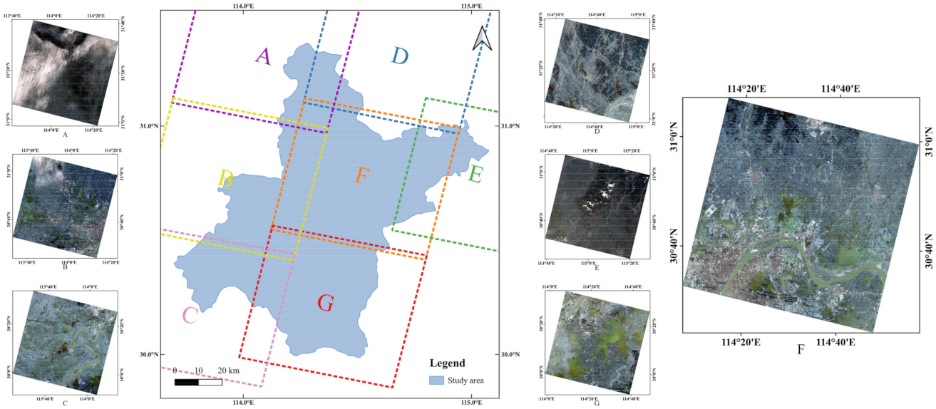
The study area and the GaoFen-1 D dataset (A, B, C, D, E, and G are used for training and F is used for testing).
Remotesensing 13 04576 g001
Figure 2. 
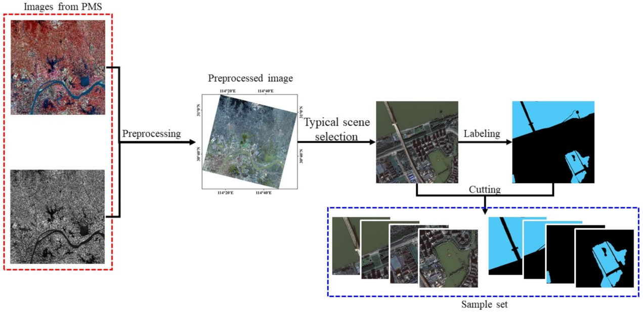
Steps of sample generation.
Remotesensing 13 04576 g002
Figure 3. 
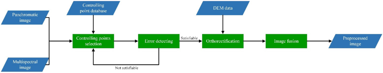
Flowchart of remote sensing image preprocessing.
Remotesensing 13 04576 g003
Figure 4. 
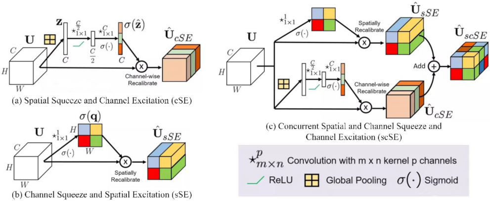
The structure of Squeeze and Excitation (SE) blocks. (ac) are the structures of cSE, sSE, and scSE, respectively.
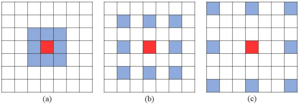
Remotesensing 13 04576 g004
Figure 5. (ac) Convolution kernels with different dilation rates of 0, 1, and 2, respectively.
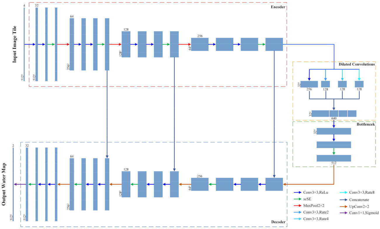
Remotesensing 13 04576 g005
Figure 6. The structure of the Lightweight Multi-Scale Land Surface Water Extraction Network (LMSWENet).
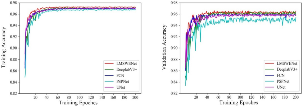
Remotesensing 13 04576 g006
Figure 7. The accuracy curves of training and validation.
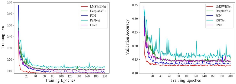
Remotesensing 13 04576 g007
Figure 8. The loss curves of training and validation.
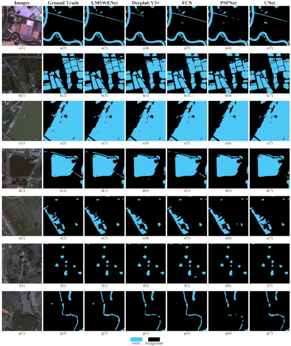
Remotesensing 13 04576 g008
Figure 9. Land surface water information extraction results for different water types. (a(1)) is the raw image of artificial ditches; (a(27)) are the water areas extracted from (a(1)) using manually labeling, LMSWENet, DeeplabV3+, FCN, PSPNet, and UNet, respectively; (b(1)–g(7)) are the water areas extracted from various types of water with agricultural water, riverside, lakes, open pools, puddles, and tiny streams, respectively.
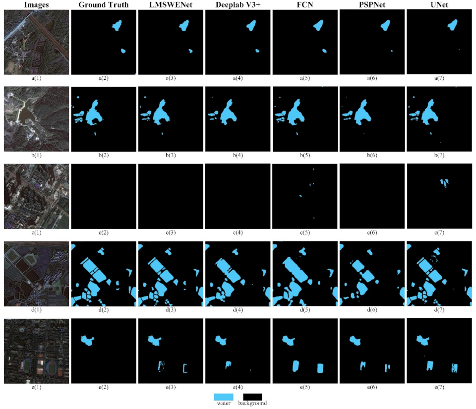
Remotesensing 13 04576 g009
Figure 10. Land surface water information extraction results in a confusing area. (a(1)) is the raw image of highways; (a(27)) are the water areas extracted from (a(1)) using manually labeling, LMSWENet, DeeplabV3+,FCN, PSPNet, and UNet, respectively; (b(1)–e(7)) are the water areas extracted from different surface environments with mountain shadows, architecture shadows, agricultural land, and playgrounds, respectively.
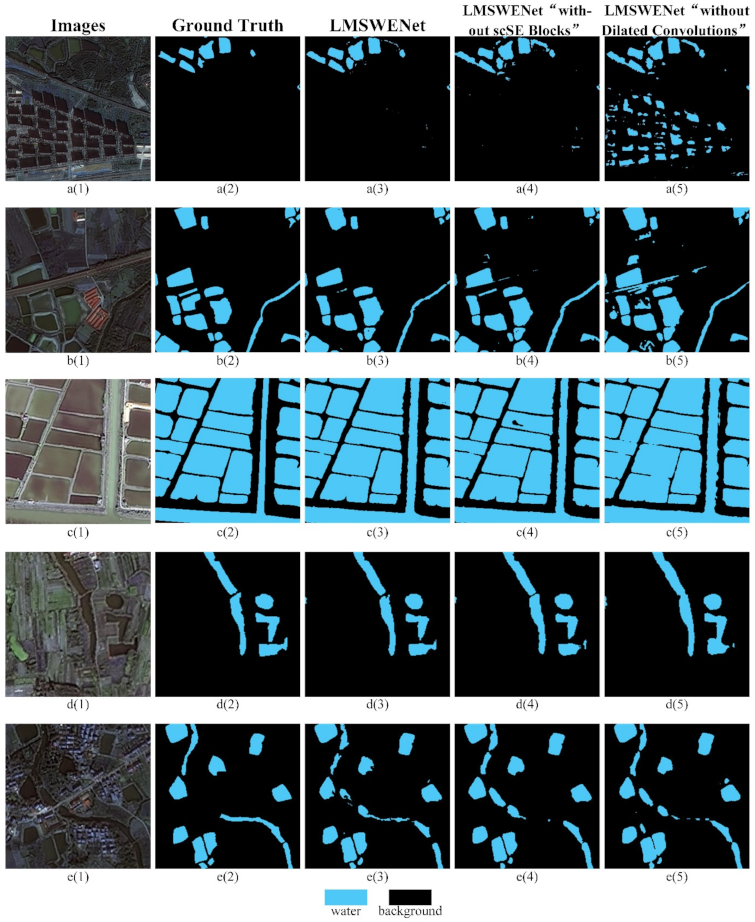
Remotesensing 13 04576 g010
Figure 11. Land surface water information extraction results for LMSWENet, LMSWENet “without scSE Blocks”, and LMSWENet “without Dilated Convolutions”. (a(1)) is the raw image of architecture shadows, and (a(25)) are the water areas extracted from (a(1)) using manually labeling, LMSWENet, LMSWENet “without scSE Blocks”, and LMSWENet “without Dilated Convolutions”, respectively; (b(1)–e(7)) are the water areas extracted from geography scenes with highways, ponds, small puddles, and rivers, respectively.
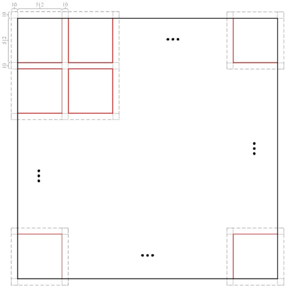
Remotesensing 13 04576 g011
Figure 12. The principle of the “sliding window” prediction method.
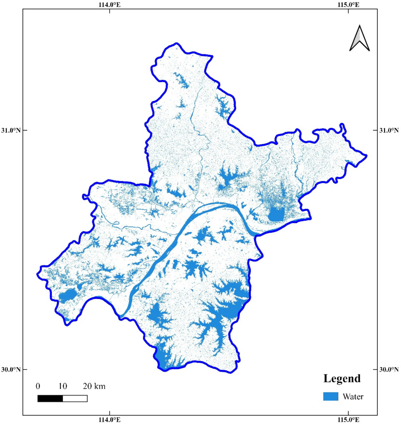
Remotesensing 13 04576 g012
Figure 13. Land surface water map of Wuhan for 2020 (LSWMWH-2020).
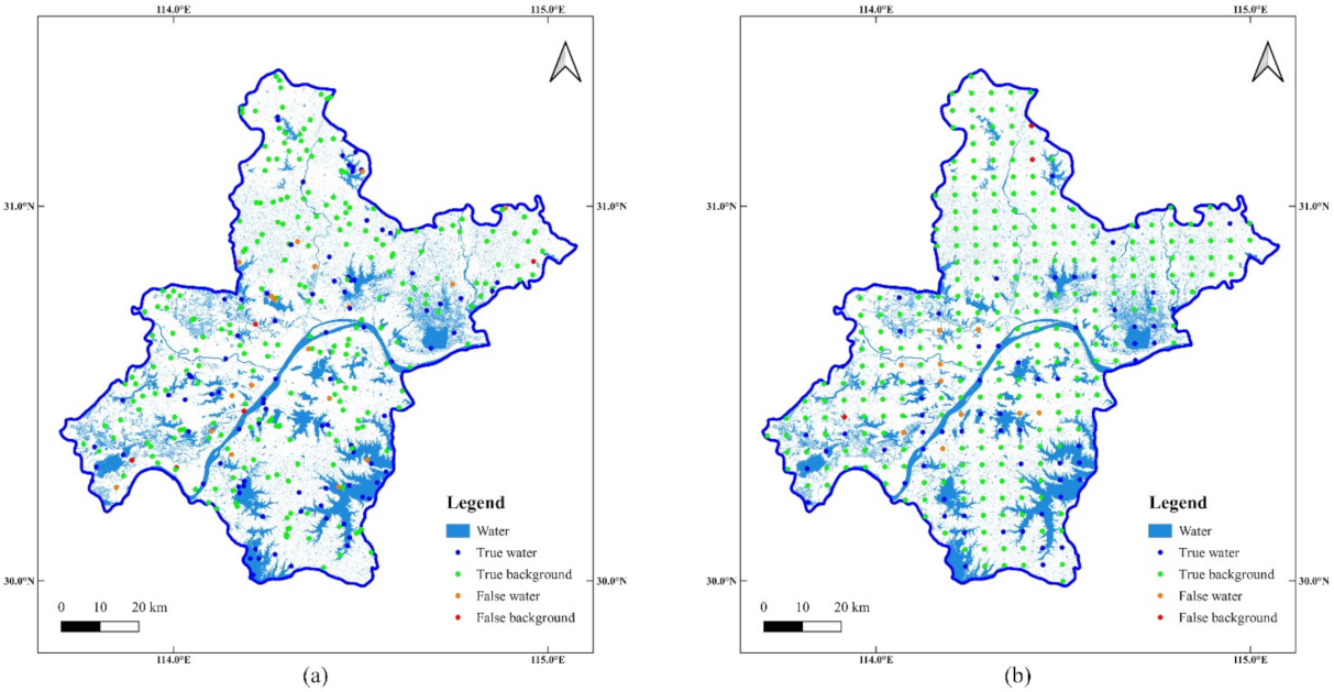
Remotesensing 13 04576 g013
Figure 14. The distribution of validation points in Wuhan. (a,b) are the distributions of random validation points and equidistant validation points, respectively.
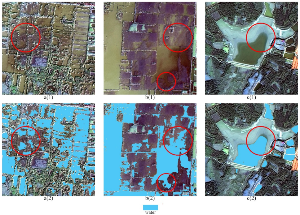
Remotesensing 13 04576 g014
Figure 15. Border area of water and non-water and the water extraction results. (a(1),b(1)) and are the raw image of ponds mixed with vegetation and sediment; (a(2),b(2)) are the water areas extracted from (a(1),b(1)) using LMSWENet; (c(1),c(2)) are the raw image of wetland and the water extraction result.
Remotesensing 13 04576 g015
Table 1. Recent methods for land surface water extraction.
CategoryExtraction Method of Land Surface Water
Threshold algorithmThreshold value of single wave band [8]
Law of the spectrum relevance [9,10]
Index of water body [15,16,17]
Machine learningSupport vector machine [22]
Maximum likelihood classification [19]
Decision tree [20]
Random forest [23]
Deep learningConvolutional neural network [13,14]
Table 2. Notation and symbols used in this paper.
SymbolDescription
U The input image.
u i The feature map of the i t h channel of an input image.
H ,   W H = Hight of a feature map, and W = Width of a feature map.
z A descriptor encoding the global spatial information.
c The channel dimensions of feature maps
i , j The spatial location of a point in the feature map.
z ^ The vectors obtained through two cascaded fully connected layers
w 1 , w 2 Weights of two fully-connected layers.
δ . The ReLu function
σ . The Sigmoid function.
F c S E U The mapping between U and U ^ c S E .
U ^ c S E The tensor after spatial-dimension recalibration.
u i , j A vector in spatial position (i, j) along all channels
q A projection tensor representing the linearly combined representation.
W s q The weight of a convolutional layer.
F s S E U The mapping between U and U ^ s S E .
U ^ s S E The tensor after spatial-dimension recalibration.
U ^ s c S E The concatenation of U ^ c S E and U ^ s S E .
Table 3. Detailed information of the study data.
ImagesCentral Longitude (°E)Central Latitude (°N)Imaging Time
(M-D-Y)
Image Size (pixel×pixel)Image Usage
A114.131.311-09-202041,329 × 40,988Training
B114.030.811-09-202041,335 × 40,983Training
C113.830.211-09-202040,004 × 39,643Training
D114.731.311-13-202041,188 × 40,839Training
E115.130.810-11-202041,070 × 40,715Training
G114.430.211-13-202041,224 × 40,854Training
F114.530.811-13-202041,211 × 40,876Testing
Table 4. Training parameters of CNNs.
ParameterValue
Loss functionMean cross-entropy
OptimizerAdam
Learning rate0.001, reduce to 1/2 of the previous every ten epochs
Batch size4
Train epoch200
Table 5. Eight evaluation criteria for the accuracy assessment.
Accuracy Evaluation CriteriaDefinitionFormula
PAThe ratio of the correctly predicted pixel numbers to the total pixel numbers P A = T P + T N T P + T N + F P + F N
ERThe ratio of erroneously predicted pixel numbers to the total pixel numbers P A = F P + F N T P + T N + F P + F N
WPThe ratio of the number of correctly predicted water pixels to the number of the labelled water pixels W P = T P T P + F P
MPThe mean Precision for all classes (water and background) M P = 1 n + 1 i = 0 n T P T P + F P
WIoUThe ratio of the intersection to the union of the ground truth water and the predicted water area W I o U = T P T P + F N + F P
MIoUThe mean IoU for all classes (water and background) M I o U = 1 n + 1 i = 0 n T P T P + F P + F N
RecallThe proportion of the number of correctly predicted water pixels and the number of the actual target feature pixels R e c a l l = T P T P + F N
F1-ScoreThe harmonic means for water precision and recall F 1 S c o r e = 2 × W P × R e c a l l W P + R e c a l l
Where TP, TN, FN, and FP refer to the numbers of pixels of true water, true background, false background, and false water, respectively.
Table 6. The efficiency comparison of the CNNs.
CNNNumber of Trainable
Parameters (Million)
FLOPs(G)Training Time
(s/epoch)
LMSWENet11.3549.2465.63
DeeplabV3+26.7154.8082.53
FCN18.6480.5675.64
PSPNet17.46117.2878.86
UNet17.27160.6072.53
Table 7. Land surface water information extraction accuracy of the CNNs.
CNNPAERWPIMPIWIoUMIoURecallF1-Score
LMSWENet98.23%1.77%98.17%98.16%92.33%94.99%93.94%96.01%
DeeplabV3+97.85%2.15%97.55%97.63%91.10%94.12%93.27%95.34%
FCN97.96%2.04%98.52%98.08%91.43%94.36%92.71%95.52%
PSPNet97.29%2.71%95.57%96.63%88.99%92.70%92.81%94.17%
UNet98.07%1.93%98.29%98.09%91.76%94.60%93.25%95.70%
Table 8. Land surface water information extraction accuracy of LMSWENet, LMSWENet “without scSE Blocks” and LMSWENet “without Dilated Convolutions”.
CNNPAERWPIMPIWIoUMioURecallF1-Score
LMSWENet98.23%1.77%98.17%98.16%92.33%94.99%93.94%96.01%
LMSWENet “without scSE Blocks”97.95%2.05%98.74%98.15%92.29%94.74%93.39%95.99%
LMSWENet “without Dilated Convolutions”97.35%2.65%98.70%97.76%88.90%92.70%89.95%91.98%
Table 9. Confusion matrix for mapping.
Type of Validation Point Classification Data
WaterNot WaterTotal
Random validation pointsReference dataWater9119110
Not water5235240
Total96254350
Equidistant validation pointsWater641074
Not water4266270
Total68276344
Table 10. Accuracy assessment for mapping.
Type of
Validation Point
PAERWPIMPIWIoUMIoURecallF1-Score
Random validation points93.14%6.86%82.73%90.32%79.13%84.93%94.79%88.35%
Random validation points95.93%4.07%86.45%92.50%82.05%88.53%94.12%90.14%
Publisher’s Note: MDPI stays neutral with regard to jurisdictional claims in published maps and institutional affiliations.

