A Neural Network-Based TEC Model Capable of Reproducing Nighttime Winter Anomaly

Abstract

With the availability of fast computing machines, as well as the advancement of machine learning techniques and Big Data algorithms, the development of a more sophisticated total electron content (TEC) model featuring the Nighttime Winter Anomaly (NWA) and other effects is possible and is presented here. The NWA is visible in the Northern Hemisphere for the American sector and in the Southern Hemisphere for the Asian longitude sector under solar minimum conditions. During the NWA, the mean ionization level is found to be higher in the winter nights compared to the summer nights. The approach proposed here is a fully connected neural network (NN) model trained with Global Ionosphere Maps (GIMs) data from the last two solar cycles. The day of year, universal time, geographic longitude, geomagnetic latitude, solar zenith angle, and solar activity proxy, F10.7, were used as the input parameters for the model. The model was tested with independent TEC datasets from the years 2015 and 2020, representing high solar activity (HSA) and low solar activity (LSA) conditions. Our investigation shows that the root mean squared (RMS) deviations are in the order of 6 and 2.5 TEC units during HSA and LSA period, respectively. Additionally, NN model results were compared with another model, the Neustrelitz TEC Model (NTCM). We found that the neural network model outperformed the NTCM by approximately 1 TEC unit. More importantly, the NN model can reproduce the evolution of the NWA effect during low solar activity, whereas the NTCM model cannot reproduce such effect in the TEC variation.

1. Introduction

The Earth’s ionosphere is a medium that contains electrically charged particles. The ionosphere is ionized by solar radiation, and its state is constantly varying due to ever-changing space weather conditions. During daytime, there is more solar radiation, which leads to photoionization and hence more ionized particles. During nighttime, the photoionization process is absent due to the lack of sunlight, which leads to reduced electron density in the ionosphere. In the ionosphere there exists enough ionization to affect the propagation of radio waves [1] (p. 1). Global Navigation Satellite Systems (GNSS) use radio waves to estimate positions on Earth and in space. Depending on the state of the ionosphere, radio waves experience a delay in their signal. The ionospheric state can be described by the Total Electron Content (TEC), commonly measured in TEC Units (TECU). One TECU stands for 10¹⁶ free electrons in a column of one squared meter. The propagation delay is directly proportional to the ionospheric TEC, which increases with an increase in electron density. The ionosphere is a dispersive medium, meaning that the delay also depends on the frequency of the radio waves. Utilizing this property, ionospheric delay can be corrected by combining two or more GNSS signals. Only higher order effects/terms remain in such combinations that are below 1% of the total delay [2]. However, single frequency users need external information or ionospheric models to correct this propagation effect.

There are models available that contain corrections for the ionosphere, such as the Klobuchar model [3,4], the NeQuickG model [5,6], or different versions of the Neustrelitz TEC Model (NTCM) [7,8,9,10,11] applicable for GPS and Galileo systems. GNSS satellites transmit coefficients as part of the navigation message to broadcast ionospheric models. The accuracy of position estimates improves when the broadcast models are applied. The International GNSS Service (IGS) releases Global Ionosphere Maps (GIMs) that contain Vertical Total Electron Content (VTEC) data. The GIMs are available in the IONosphere EXchange Format (IONEX) as rapid and final solutions, both released with a latency. The rapid solution is released within 24 h, but the final solution has a latency of approximately 11 days. The GIMs are more accurate than the broadcast models [12] and have been available since the official start of 1998. Besides empirical ionosphere models, there are first-principle physics models that have the potential to provide ionospheric forecasts. Examples of such models are the Thermosphere-Ionosphere-Electrodynamics General Circulation Model (TIE-GCM) developed at the National Center for Atmospheric Research (NCAR), or the Coupled Thermosphere Ionosphere Plasmasphere Electrodynamics Model (CTIPe) developed at the Space Weather Prediction Center from the National Oceanic and Atmospheric Administration (NOAA). However, Shim et al. [13] have suggested that errors in electron density can be very large due to errors in initialization and boundary conditions.

Different versions of NTCM developed at the German Aerospace Center (DLR) have shown that the computationally very fast 12 coefficient model is comparable in its simplicity to the Klobuchar model and achieves a similar performance as the NeQuick2/NeQuickG model [7,9,10,11,14]. The NTCM approach describes the TEC dependencies on local time, geographic/geomagnetic location, and solar irradiance and activity. The local time dependency is explicitly described by the diurnal, semi-diurnal, and ter-diurnal harmonic components. The two ionization crests at the low latitude anomaly regions on both sides of the geomagnetic equator are modelled by Gaussian functions. The 12 model coefficients are fitted to the TEC data to describe the broad spectrum of TEC variation at all levels of solar activity. The driving parameter of the model is either the daily solar radio flux index, F10.7, which is a proxy for the EUV radiation of the Sun, or the ionosphere correction coefficients transmitted via GPS or Galileo satellite navigation messages.

The NTCM models are developed based on TEC data provided by the Center for Orbit Determination in Europe (CODE) [15]. The models can predict the mean TEC behavior and reduce the ionospheric propagation errors by up to 80% in GNSS applications [8]. The persistent anomaly features that exist during both high and low solar activity times, such as the equatorial ionization anomaly (EIA), are modelled by NTCM approaches. However, the anomalies that become visible only during low solar activity (LSA) time, such as the Nighttime Winter Anomaly (NWA), the Weddell Sea anomaly, and the midsummer nighttime anomaly (MSNA), are not explicitly modelled. The NWA is present because during LSA periods the mean ionization level is higher in the winter nights compared to the summer nights [16]. During the day, the ionization is equal or even less compared to the summer, and thus, the NWA is only visible during the night. Modelling NWA and MSNA features are out of scope when developing empirical TEC models with a limited number of model coefficients. However, with the availability of fast computing machines, as well as the advancement of machine learning techniques and Big Data algorithms, the development of a more sophisticated TEC model featuring the NWA and other effects is possible and is presented here.

The use of neural networks (NN) for predicting TEC is not new; various types of networks capable of predicting TEC have already been developed. Some of the networks are focused on regional or short-term predictions, or are trained with data from a short period, which does not cover all solar activity. A few examples of previously developed networks are the Long Short-Term Memory (LSTM) network proposed by Xiong et al. [17] that can make accurate, short-term TEC predictions over China, or the model proposed by Machado and Fonseca Jr. [18] that forecasts the VTEC of a subsequent 72 h in the Brazilian region. A combination of Convolutional Neural Networks (CNNs) and LSTM networks has been proposed by Cherrier et al. [19] This approach is able to predict global TEC maps 2 to 48 h in advance. The TensorFlow-based, fully connected NN prediction model proposed by Orus Perez [12], the IONONet, was trained with GIM data from LSA periods and was also tested with LSA data. The IONONet has been making global predictions one or more days ahead but is unable to represent the equatorial anomalies. However, the IONONet model adjusted with NeQuick2 is able to represent the equatorial anomalies. The NN approach introduced by Cesaroni et al. [20] trains a neural network with data from one solar cycle on a selection of grid points and uses the NeQuick2 model to extend it to a global scale. The approach proposed here is a fully connected neural network trained with global GIM data from almost two solar cycles.

Most of the previously mentioned models developed using machine learning techniques are already able to predict VTEC maps containing large-scale features, but a prediction containing NWA features is newly developed. The paper is divided into sections, beginning with brief descriptions of the ionospheric TEC models. The subsequent section discusses the database and sources used for the datasets for model development and testing. The final section provides a performance evaluation of the proposed NN model compared to the NTCM model. The model is further evaluated with respect to its capability of reproducing the NWA feature during low solar activity time.

2. Database

The database used to train and test the proposed neural network consists of GIMs provided by the CODE [15]. The daily IONEX files were downloaded from the Crustal Dynamics Data Information System (CDDIS) archive at https://cddis.nasa.gov/archive/gnss/products/ionex/ (accessed on 30 March 2021). Each IONEX file contains either bi-hourly or hourly (since the end of 2014) VTEC maps with 2.5° and 5° latitude and longitude resolution. We used CODE data from 2001 to 2020, which includes high and low solar activity condition/levels covering the last two solar cycles, 23 and 24.

The solar activity level was provided by the solar radio flux index, F10.7, measured in solar flux units (sfu, 1 sfu = 10–22 Wm⁻²Hz⁻¹). This describes the solar emission at a wavelength of 10.7 cm [21]. The daily F10.7 data were obtained from NASA’s (National Aeronautics and Space Administration) OMNIWeb interface, available at https://omniweb.gsfc.nasa.gov/form/dx1.html (accessed on 12 May 2021). A time series of F10.7 is plotted in Figure 1, which varies from about 70 units at LSA to up to more than 200 units at high solar activity (HSA) conditions, causing high dynamics in the VTEC.

In order to reduce computational complexity, the datasets (e.g., F10.7, VTEC maps) were downscaled by taking the Carrington rotation averages at each hour. One Carrington rotation period is approximately 27 days, the time for which a fixed feature of the Sun rotates to the same apparent position as viewed from Earth. Each rotation of the Sun is given a unique number, called the Carrington Rotation Number, starting from 9 November 1853 [22]. The average F10.7 for each Carrington rotation is plotted in Figure 1 (see orange plot) for the considered period. We observe that the average F10.7 successfully follows the trend of the solar activity level.

First, we divided the data into two main categories: training and test datasets. The training data consisted of data from the years 2001 to 2019, excluding the year 2015. The testing dataset consisted of data from the years 2015 and 2020, which corresponded to high and low solar activity conditions, respectively. The data from the December 2019 period were excluded from the training dataset since they were used for analyzing the model performance during the NWA condition.

The spatial resolution of the VTEC maps was reduced to speed up the model training. A resolution of 2.5° latitude by 15° longitude was used for the training dataset. However, for model testing, the original data (i.e., individual hourly maps of 2.5° and 5° latitude and longitude) as well as the Carrington rotation averaged data were used.

Since a validation dataset is needed to find the correct free parameters, known as the hyperparameters, part of the training data was separated. The process of finding the optimized free parameters is called hyperparameter tuning. Not only is the structure of the network defined by the hyperparameters (i.e., the number of neurons or layers), but they also define how the network is trained (i.e., the learning rate or number of epochs).

If the cost function (mean squared error) decreases for only the training set and not for the validation set, it means that the model is learning noise in the training data [23]. The chosen hyperparameters are discussed in the method section. After finding the correct hyperparameters, the model was trained one last time with the validation dataset included in the training dataset.

The data were normalized and scaled to an interval of [0,1] in order to converge the model faster using the MinMaxScaler function from the Scikit-Learn Python library [24]. The scaler was fitted to the training and validation data. The testing data were left out because, otherwise, the scaler could extract information from the test set. After the scaler was fitted, the test data could be transformed by the scaler in order to make predictions. If the information of the test datasets was used before or during training, the model’s performance could not be fairly evaluated as information about the test dataset may leak into the training of the model.

3. Method

Our previous investigation and modelling activities (e.g., [7,8,9,10,11]) show that the ionospheric TEC can be successfully modelled by describing TEC dependencies on local time, seasons, geographic/geomagnetic location, solar irradiance, and activity. Our current investigation shows that the same geophysical conditions can be selected as features for training a neural network to accurately describe the events of the ionospheric TEC. Therefore, we used the following six features: F10.7 index, solar zenith angle, day of year (DOY), Universal Time (UT), geographic longitude, and geomagnetic latitude. UT was selected instead of Local Time (LT), although in our previous modelling activities LT was always used. We found that with neural network-based modelling we could directly use UT without any performance degradation. The solar zenith angle is the angle between the Sun’s rays and the vertical direction at a geographic location. The solar zenith angle dependency (Φ) is considered by the following expression [25]:

$$\cos \mathsf{\Phi } = \sin \mathsf{\varphi } \ast \sin \mathsf{\delta } + \cos \mathsf{\varphi } \ast \cos \mathsf{\delta } \ast \cos \left(\mathrm{LT}\right)$$

(1)

where ϕ is the geographic latitude and δ is the solar declination.

The International Geomagnetic Reference Field (IGRF) model [26] was used for geographic to geomagnetic latitude conversion.

At what extent the selected features correlate to the TECs can be known by estimating a Pearson’s correlation matrix [27], shown in Figure 2. We found that the F10.7 index and the solar zenith angle had a moderate to high correlation with the VTEC, whereas other features showed relatively low correlation values.

The prediction of VTEC is a regression problem for which a fully connected neural network is used to train the model. The architecture was built with a sequential model using the open source TensorFlow [28] and Keras [29] libraries, written for Python. Keras was built on top of TensorFlow and was designed to make the implementation easier. A 6-256-128-64-32-16-1 network architecture was chosen, where the numbers represent the number of neurons of each layer. This architecture is similar to one of the model architectures investigated by Orus Perez [12]. A schematic view of the network architecture is displayed in Figure 3.

To map non-linearities, the Rectified Linear Unit (ReLU) activation function was used. ReLU returns zero in the case of a negative input and returns a value for positive inputs. ReLU is a widely used activation function due to its computational efficiency [30]. All the hidden layers of the network use the ReLU activation function. The output layer uses a linear identity activation function.

During the training of a network, it can occur that the model remembers the training data too well, which is called overfitting. This means that the model has also learnt the noise of the training dataset, and the performance of the model on the validation and testing datasets may be lower. One of the ways to avoid overfitting is by adding a regularization term that penalizes the model for fitting the data too well. As already mentioned, the model’s training data consisted of Carrington averaged data. Instead of being fed daily data, the model was fed Carrington averaged values (approximately 27 days), making it less vulnerable to noise. There was no regularization term added because, otherwise, the model would not be able to detect small-scale features such as the NWA.

The model training was optimized using an optimization method called Adam [31], which considers a learning rate of 0.0001 and the Mean Squared Error (MSE) as the loss function. The Adam optimizer minimizes the MSE and is a computationally effective algorithm with little memory requirements [31]. The loss function is defined as the MSE between model prediction and VTEC from the GIMs, also known as label. The training process took several hours, which can be considered as short since no special hardware was used other than a personal computer with an Intel Core i7-8665U CPU and 16 GB RAM. The number of epochs used for the model’s training was 150, which stands for how many times the complete training dataset is passed through the network. The model was fitted using a batch size of 128. The batch size is the number of samples that are being fed to the network.

The first consideration was using two models, one for HSA conditions (e.g., F10.7 > 100) and another one for LSA conditions. During high solar activity periods, equatorial anomaly crests are more prominent features when compared to low activity periods. The specialized LSA and HSA models had difficulties showing the predications that contained equatorial anomalies. The models predicted the anomalies as one blob instead of two crest features. After increasing the complexity of the network, such as by increasing the number of neurons and layers, the HSA model was able to show predictions containing the two crests. The anomalies were still not present in predictions made with the specialized LSA model because the crests were less prominent. After lowering the regularization term, the two crests became visible. However, the final model was trained on data from both solar periods and could also predict the equatorial anomalies during the LSA period. In terms of root mean square (RMS) errors, the combined model performed slightly worse than the specialized models, but the difference was not significant enough. However, a combined model is preferable for a smooth transition of TEC prediction when the main driving parameter, F10.7, experiences fluctuations due to space weather events. The NWA was more difficult to model because it is a short-lived feature. After reducing the regularization term, the model was able to make predictions containing the NWA effect.

After training, the model had to be tested with unseen test data. The model’s results were evaluated by looking at the performance metrics, such as standard deviation (STD), mean, RMS errors, and the presence of features in the VTEC predictions. The performance of the model was also compared to the performance of the NTCM model [7].

The model was validated against the test data from the HSA in 2015 and the LSA in 2020. The test dataset contained the Carrington averaged data as well as the original daily data. Model values were calculated for the same geophysical conditions as the test datasets. The differences between the model values and test datasets were computed and the statistical estimates of differences were derived. The performance of the daily data in terms of mean, STD, and RMS differences is provided in

Table 1. Quality measures of the daily test data and the Carrington averaged test set.

	Combined		2015		2020
	Daily	Carrington	Daily	Carrington	Daily	Carrington
Mean	−0.02	−0.25	0.72	−0.07	−0.75	−0.51
STD	4.56	3.00	5.95	3.74	2.28	1.31
RMS	4.56	3.01	5.99	3.74	2.40	1.40

. We found that the values were lower for the Carrington averaged data compared to the daily data. This was expected because the model was trained with Carrington rotation averaged data. The model’s performance was worse during the HSA in 2015 compared to the LSA in 2020. The VTEC values had a larger spread, and were higher during 2015, which is shown in

Table 2. Quality measures of the Global Ionosphere Maps (GIMs) and predictions.

	2015		2020
	GIMs	Predictions	GIMs	Predictions
Mean	19.36	18.64	8.13	8.88
STD	16.26	15.32	6.72	7.50
Min	0.00	0.00	0.00	0.00
Max	142.30	117.45	66.00	74.08

. Therefore, it was expected that the model would have had lower accuracy during the HSA in 2015. In Table 2, it can also be seen that the model was underpredicting during the HSA period because the model’s mean, STD, and maximum value was lower compared to the GIMs. However, during LSA conditions, the model was overpredicting because the mean, STD, and maximum value were higher compared to the GIMs. This behavior could have resulted from training the model with data from HSA and LSA periods and using Carrington rotation averaged data instead of daily data.

4. Results and Discussion

In the present work, NTCM was used as a benchmark for comparing the proposed neural network-based TEC prediction (NN) model with independent reference data. Therefore, it is interesting to compare the NTCM and NN models for whether they can show the signature of the NWA.

4.1. Comparison with NTCM

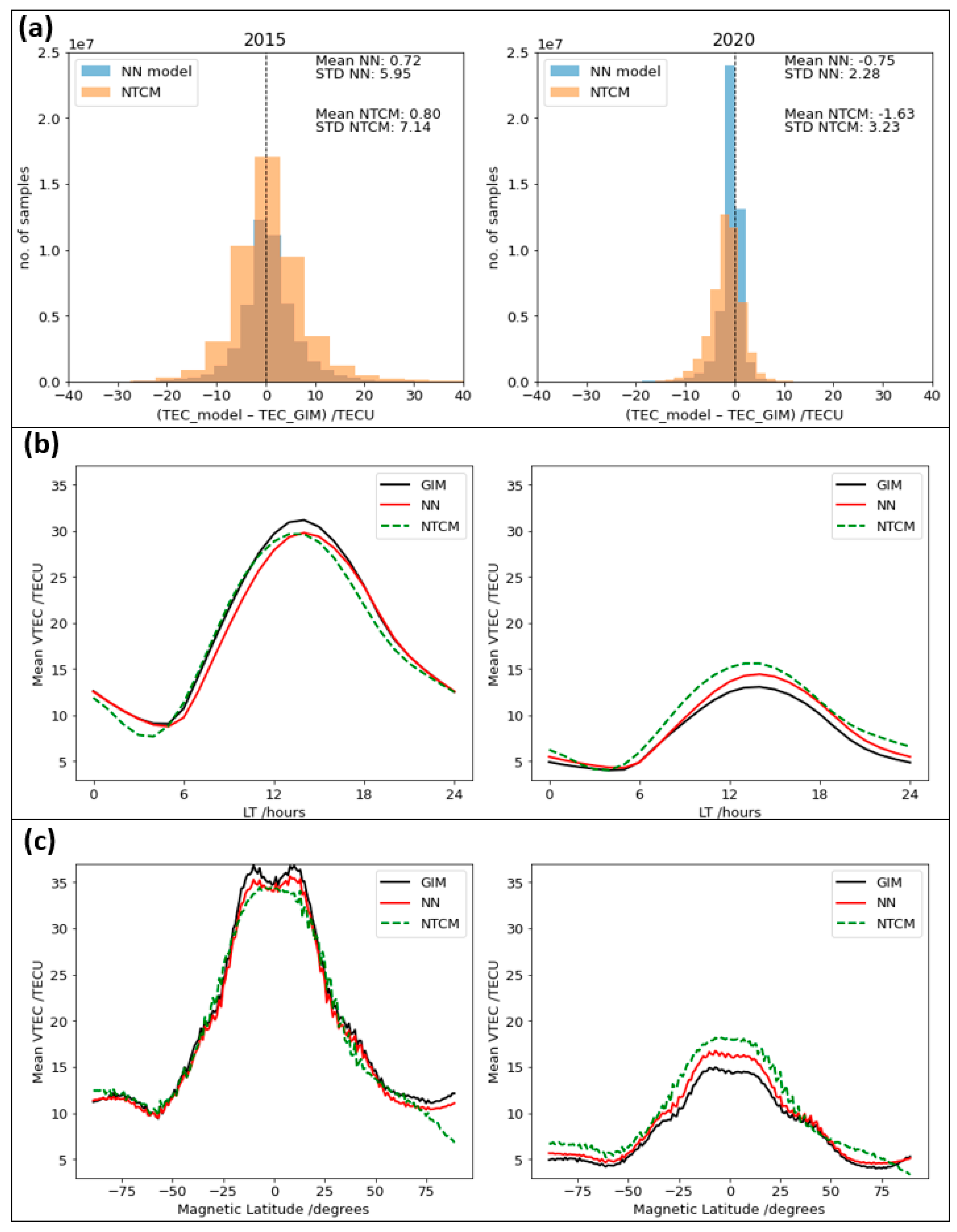
The model performances were compared in terms of histogram plots and statistical estimates of model residuals in the top panel of Figure 4. We found that the mean residuals were approximately equal for both models for the HSA in 2015, whereas the STD residual was about 1.2 TECU less for the NN model (see top-left plot). However, during the LSA in 2020, both mean and STD values were about 1 TECU less for the NN model compared to the NTCM.

The average diurnal variation of TEC as found in the GIMs and predicted by NN and NTCM are shown in the middle panel of Figure 4 for both LSA (see middle-right) and HSA years (middle-left panel). The VTEC reached its maximum at around 14–15 LT and decreased gradually with the increase in LT. The largest differences between the reference VTEC values and predictions were found around the VTEC maximum at about 14 LT, when the effect of the ionosphere was most prominent. In the HSA diurnal variation plot (year 2015), the NTCM model was closer to GIM data during the morning LT hours, but in the afternoon the NN model’s VTEC predictions were closer. In the LSA of 2020, the NN model predictions were closer to the GIMs for almost all LT hours. From the plots in Figure 4, it can be seen that the VTEC predicted by the NN was in most cases closer to the GIM data, especially during the LSA year.

Solar activity has an influence on VTEC values, which are higher during HSA conditions compared to LSA periods. According to Adewale et al. [32], the VTEC increases from 6 LT and the maximum is reached at approximately 14–15 LT. The diurnal variation of the ionosphere has a wave-like pattern, meaning the VTEC increases during daytime and decreases during the night. It occurs every 24 h and is caused by the rotation of the Earth around its axis. This behavior is previously seen in the predictions shown in the middle panel of Figure 4. In the bottom panel of Figure 4, the VTEC is plotted against the geomagnetic latitude. From these plots it can be seen that the NN model was closer to the GIM values for both testing years compared to the NTCM. We found that the north and south crest separation was visible in the NN model during the HSA year, whereas it was not visible in the NTCM.

4.2. Presence of NWA Signature

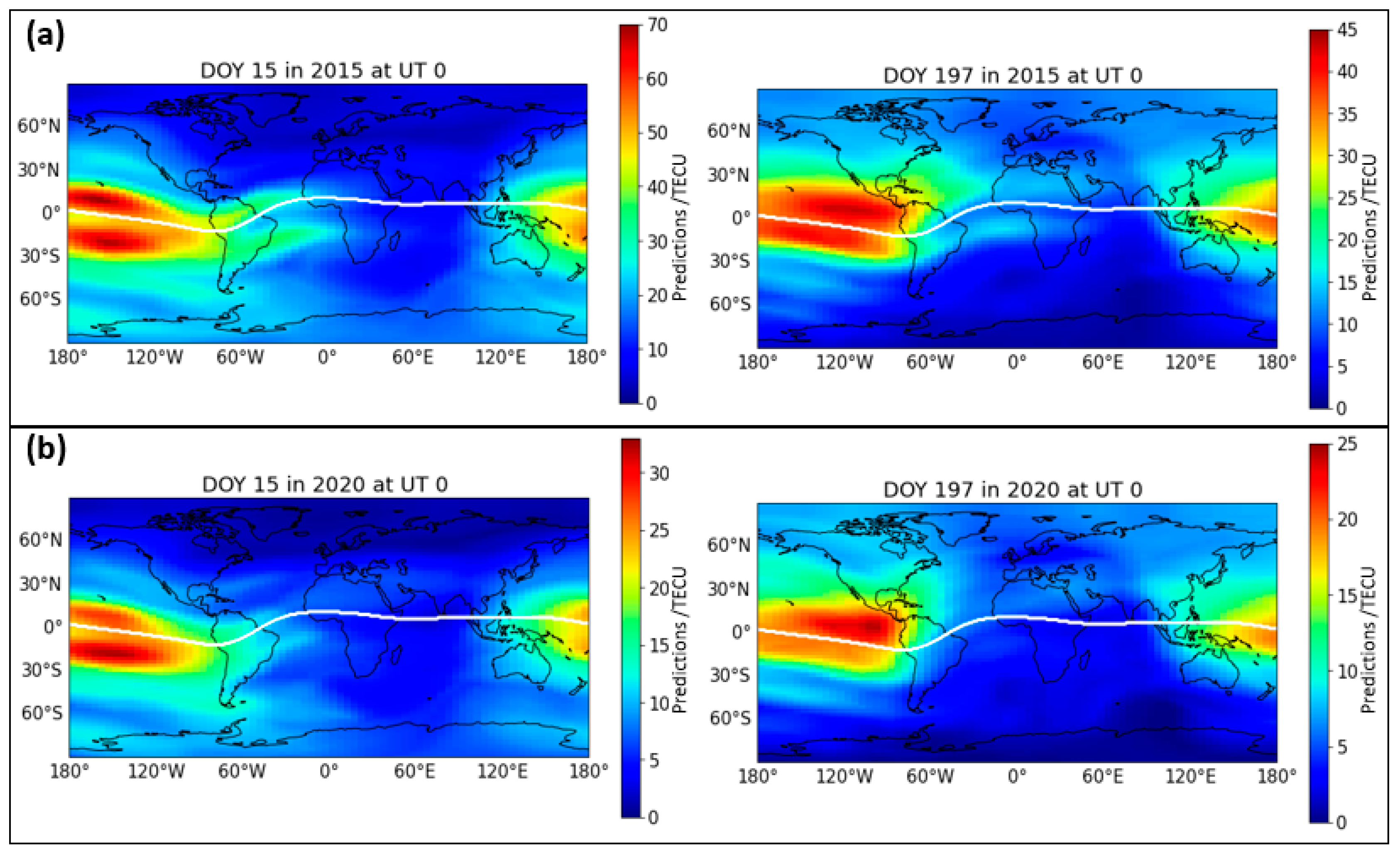
Before investigating the presence of the NWA feature, we first investigated the NN model’s ability to predict the common seasonal variations, such as the presence of higher TEC values during the summertime in the corresponding hemisphere. For this purpose, the VTEC maps at UT 0 for DOY 15 and DOY 197 are shown in Figure 5 for the HSA year (top panels) and for the LSA year (bottom panels). The DOY 15 represents a winter day in the Northern Hemisphere, whereas DOY 197 represents a summer day in the Northern Hemisphere. Note that the seasons are opposite in the Southern Hemisphere and that the color bars are different for each plot due to the difference in levels of ionization. Figure 5 clearly shows that the background ionization was higher in the hemisphere where it is summer.

The equatorial anomaly, also known as the Appleton anomaly, can be seen as two crests within ~±20 degrees magnetic latitude, also seen in Figure 5. The crests develop in the local morning hours and continue to exist even beyond the sunset [33].

The NWA is a feature that only occurs during LSA periods and nighttime in the middle latitude at certain longitude sectors. As investigated by Jakowski et al. [16,34,35], the NWA is visible in the Northern Hemisphere for the American sector and in the Southern Hemisphere for the Asian longitude sector under low solar activity conditions. During the NWA, the mean ionization level is found to be higher in the winter nights compared to the summer nights. The higher level of ionization during winter nights is caused by the transport of interhemispheric plasma from the conjugated summer hemisphere [16,35]. This happens for longitude sections where the displacement of the geomagnetic equator from the geographic equator is the largest [16], which is in the American and Asian sectors.

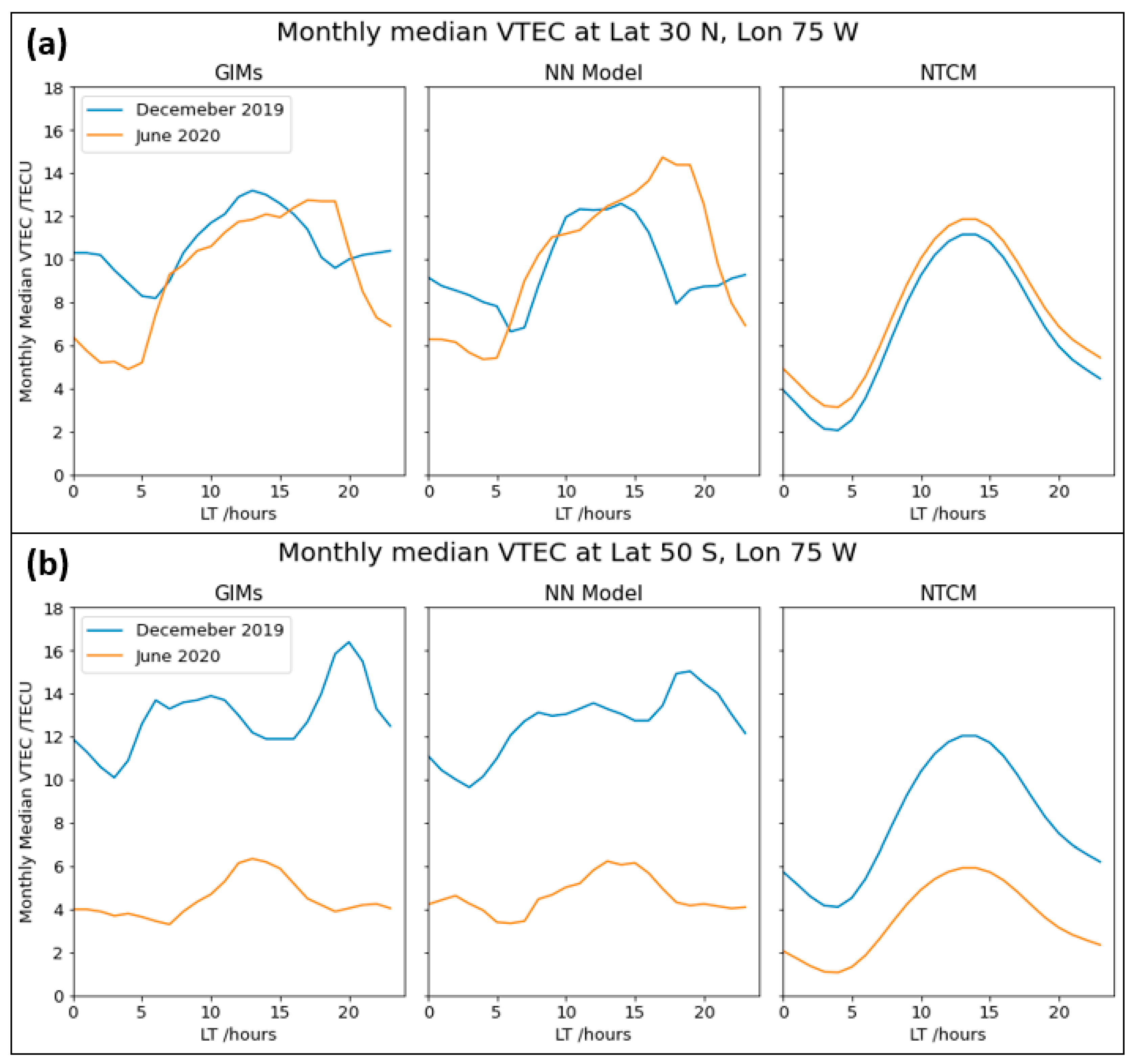
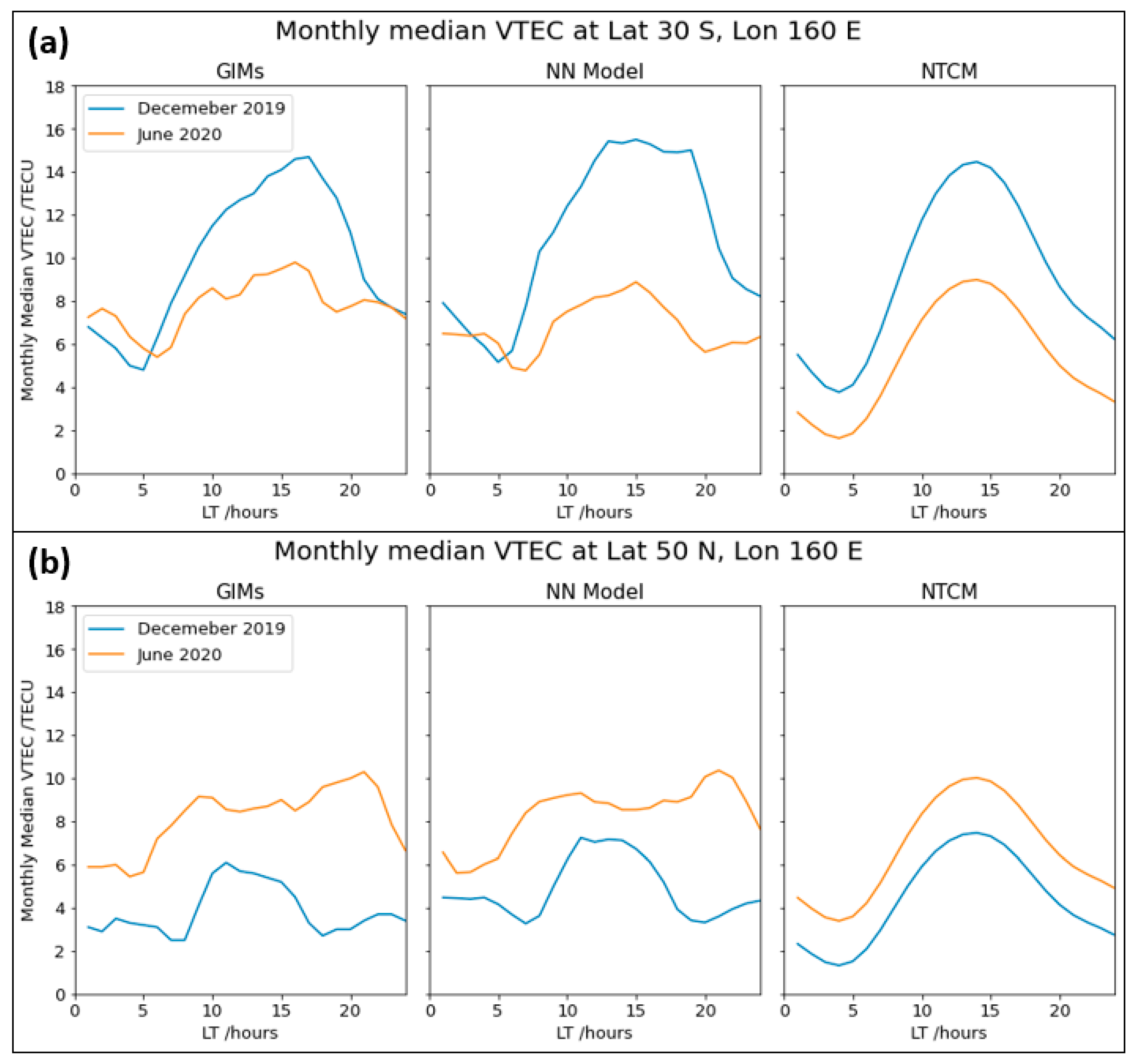
Next, we investigated the performance of our NN model in describing the NWA features. For this, the monthly median VTEC values during winter and summer months were computed at certain middle latitude locations. Figure 6 and Figure 7 show the corresponding VTEC plots as a function of the local time. We chose the same two reference geographic locations (30°N, 75°W) and (30°S, 160°E) considered by Jakowski et al. [16] for the NWA investigation. Figure 6 and Figure 7 show that the NWA effect was visible in the reference locations (see top panel plots), whereas it was not visible in the corresponding geomagnetic conjugated locations (50°S, 75°W and 50°N, 160°E) as expected. December 2019 and June 2020 were chosen as winter and summer months, respectively, for the Northern Hemisphere. The seasons are opposite in the Southern hemisphere. It should be noted that the corresponding data were not used in the NN model training.

The left panels of Figure 6 and Figure 7 show the TEC measurements, and the middle and right panels show the corresponding model results. As already mentioned, the NTCM results are included in the right panel for comparison purposes. By comparing monthly TEC variation in the top-left panel of Figure 6, we see that the nighttime (e.g., 21–5 LT) TEC values were higher during the Northern winter (see blue curve). Similarly, the top-left panel of Figure 7 shows that the nighttime (e.g., 0–5 LT) TEC values were higher during the Southern winter (orange curve). A larger TEC difference between the summer and winter months at 30°N, 75°W indicates that the NWA effect was more pronounced in the American sector than in the Asian sector. The results agree well with the results by Jakowski et al. [16] Comparing the middle and right panels with the left panel, we see that the signature of the NWA effect was visible in the NN model but not visible in the NTCM. Although the NN model showed NWA signatures, the magnitude of TEC differences between the summer and winter months was less in comparison to the observed TEC differences.

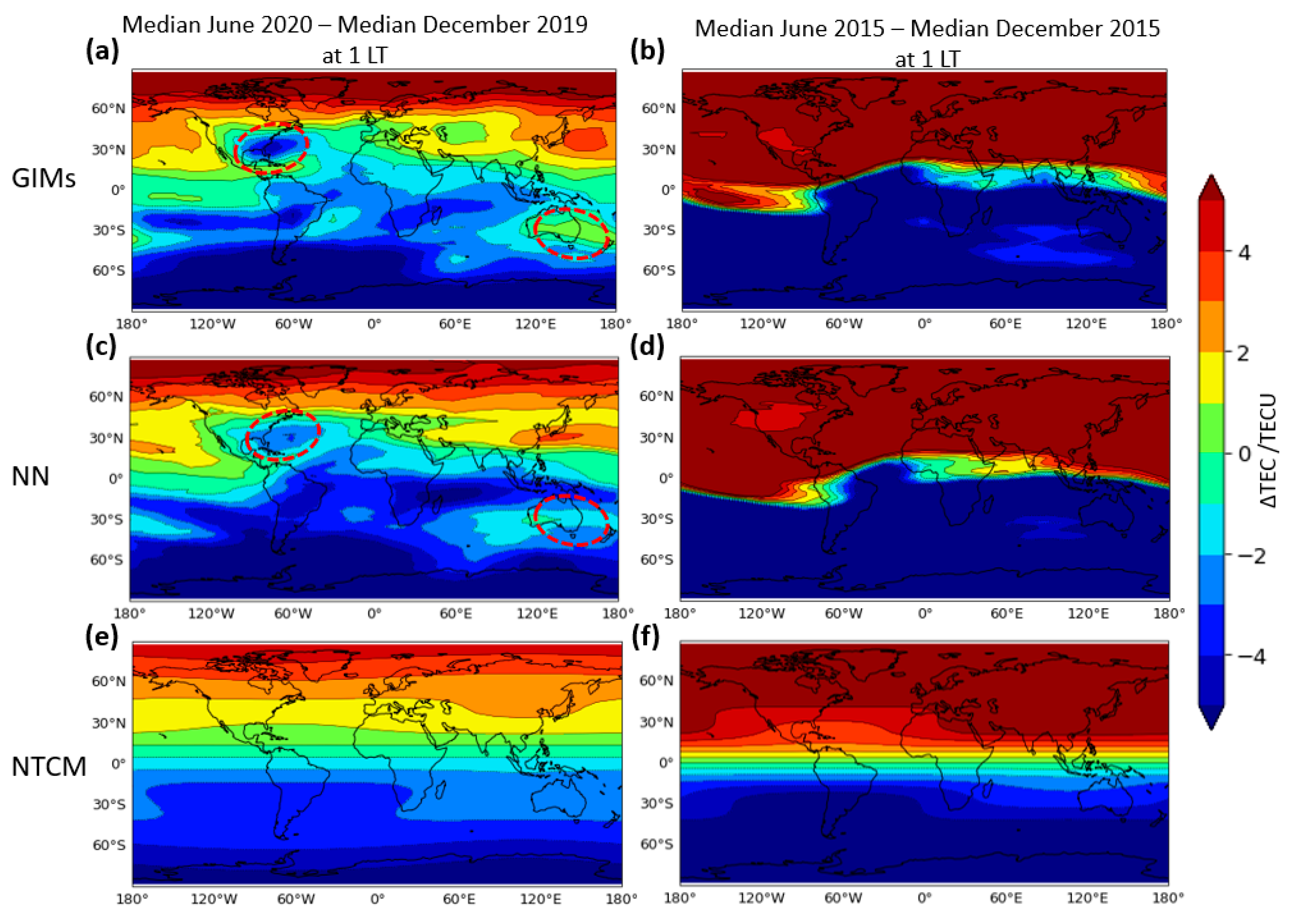
We further evaluated the presence of the NWA effect on the global ionospheric maps (GIMs) and the performance of the NN model in preserving the NWA features. For this, the monthly median TEC maps for the Northern winter months of December 2015 and 2019 were computed and subtracted from the monthly median TEC maps of the Northern summer months of June 2015 and 2020, respectively. The years 2015 and 2019 represented the HSA and LSA conditions, respectively. The top, middle, and bottom panels of Figure 8 show the TEC difference maps for the IGS GIMs, the NN model, and the NTCM model, respectively. The left panel shows the TEC differences for the LSA condition, whereas the right panel shows the TEC differences for the HSA condition.

In the GIM data (top panel), the NWA effect was visible during the LSA condition (left plot, see encircled areas) and not visible during the HSA condition as expected. The middle panel shows that the NN model successfully described the NWA features during the LSA, and such features were absent during the HSA condition. The bottom panel shows that the NTCM model could not reproduce the NWA features. Both the observations and NN model show that NWA was more prominent for the American sector in the Northern Hemisphere than for the Asian sector in the Southern Hemisphere.

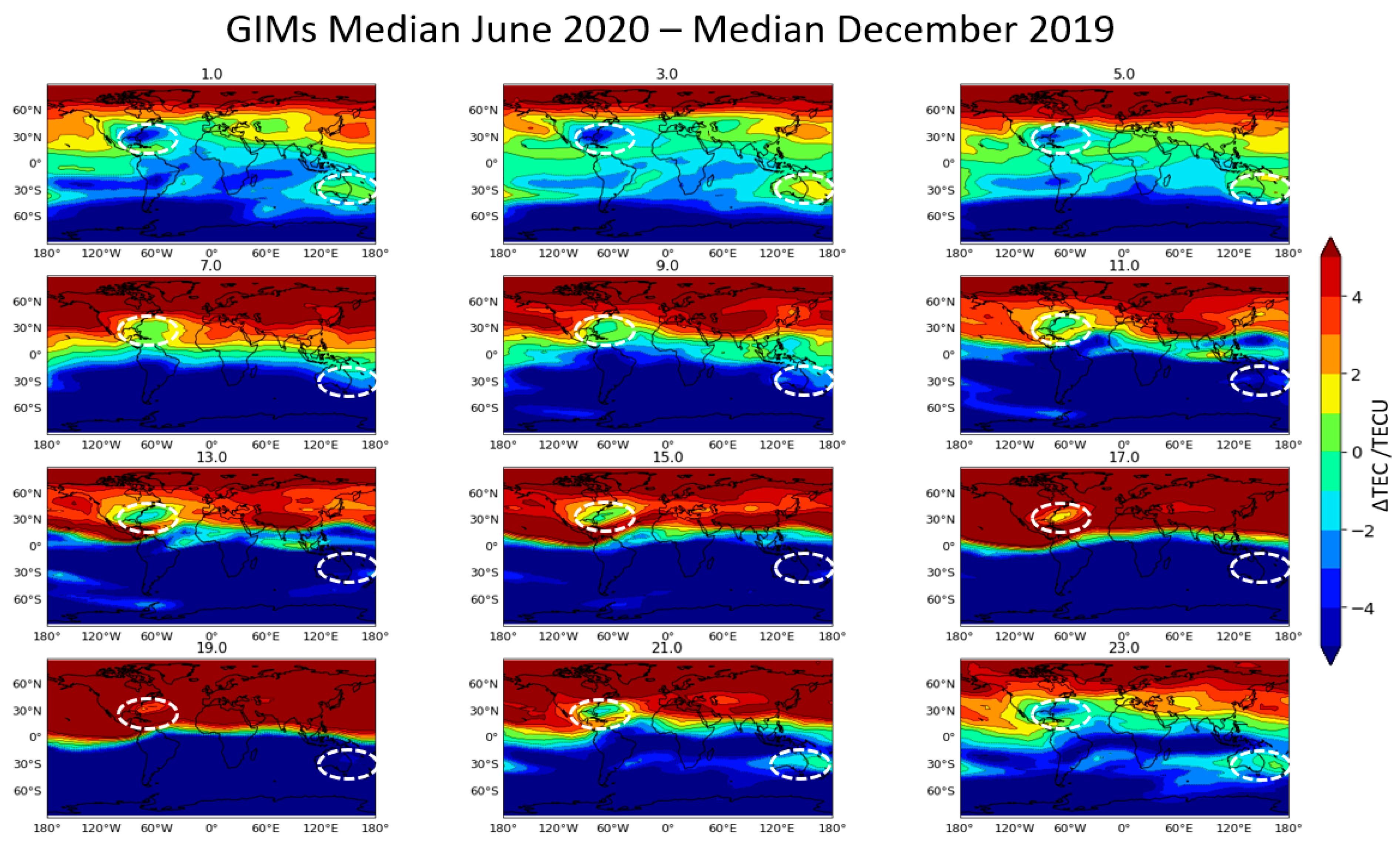
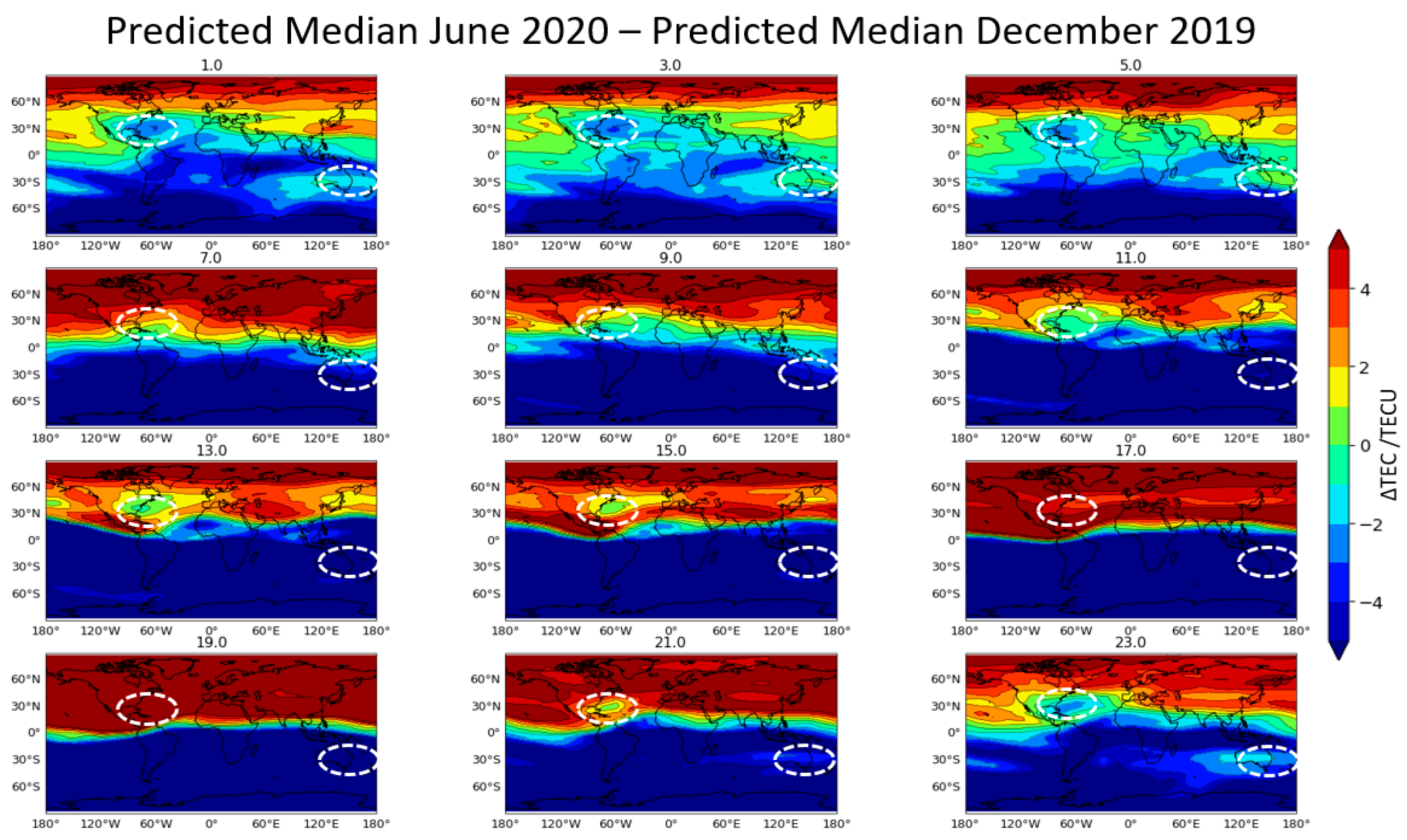
To show the formation of NWA as a function of LT on a global scale, the TEC difference maps were generated every two LT hours for IGS GIMs as well as for the NN model, shown in Figure 9 and Figure 10, respectively. To indicate the NWA, white dotted lines are displayed at the location of the NWA. We see that the NWA in the American sector appears to evolve at LT 21 until LT 5, and then gradually decreases in subsequent maps. Figure 10 shows that the NN model could successfully reproduce the evolution of the NWA during nighttime hours. The Southern Hemisphere’s NWA in the Asian sector was more strongly present during 3–5 LT, the same behavior was seen in the NN predictions. At 1 LT, the NN predictions did not clearly show the NWA in the Asian sector, even though it was present in the GIMs. A reason for this behavior could be that the Southern Hemisphere’s NWA located in the Asian sector is not very prominent in comparison to the Northern Hemisphere’s NWA. Therefore, it is harder for the model to learn it.

5. Conclusions

In this paper, a fully connected neural network-based (NN) TEC model was proposed for global Vertical TEC (VTEC) predictions that could reproduce the Nighttime Winter Anomaly (NWA). The NWA is a unique feature that only occurs at nighttime during low solar activity conditions. The model was trained with a large dataset containing IGS Global Ionosphere Maps (GIMs) from almost two solar cycles covering the years 2001 to 2019, with 2015 excluded. The NN model was tested with unseen data from a high and a low solar activity year (2015 and 2020, respectively). The day of year, universal time, geographic longitude, geomagnetic latitude, solar zenith angle, and solar activity proxy, F10.7, were used as input parameters for the network in order to predict the VTEC.

Our investigation shows that the model clearly reproduces the NWA feature in the global VTEC predictions. The Northern Hemisphere’s NWA in the American sector is clearly seen at 1 Local Time (LT), but the Southern Hemisphere’s NWA becomes more visible during 3–5 LT in the NN model prediction. The NWA in the Asian sector is also more prominent in the GIM data at 3 LT, but is also present at 1 LT. The reason why the NWA in the Asian sector is not clearly visible in the VTEC prediction is that the NWA effect is not as strong as it is in the American sector.

To validate the neural network model, a comparison with the Neustrelitz TEC Model (NTCM) was made. The NN model outperforms the NTCM by approximately 1 TEC unit in the case of high and low solar activity periods. The NTCM is not able to make predictions containing the NWA feature, whereas the NN model is able to do so. Even though the model was trained on both high and low solar activity data, it can still predict features that only occur during low solar activity periods in the night like the NWA can.

References

1. Davies, K. Ionospheric Radio; The Institution of Engineering and Technology: London, UK, 1990; p. 1. ISBN 978-0-86341-186-1. [Google Scholar]
2. Hoque, M.M.; Jakowski, N. Estimate of higher order ionospheric errors in GNSS positioning. Radio Sci. 2008, 43, RS5008. [Google Scholar] [CrossRef]
3. Klobuchar, J.A. Ionospheric Time-Delay Algorithms for Single-Frequency GPS Users. IEEE Trans. Aerosp. Electron. Syst. 1987, 23, 325–331. [Google Scholar] [CrossRef]
4. GPS Directorate. Systems Engineering & Integration Interface Specification IS-GPS-200, Revision J. 2018. Available online: https://www.gps.gov/technical/icwg/IS-GPS-200J.pdf (accessed on 1 July 2021).
5. European GNSS (Galileo) Open Service. Signal-In-Space Interface Control Document, Issue 1.3. December 2016. Available online: https://www.gsc-europa.eu/sites/default/files/sites/all/files/Galileo-OS-SIS-ICD.pdf (accessed on 25 July 2021).
6. Nava, B.; Coisson, P.; Radicella, S.M. A new version of the NeQuick ionosphere electron density model. J. Atmos. Sol. Terrest. Phys. 2008, 70, 1856–1862. [Google Scholar] [CrossRef]
7. Jakowski, N.; Hoque, M.M.; Mayer, C. A new global TEC model for estimating transionospheric radio wave propagation errors. J. Geod. 2011, 85, 965–974. [Google Scholar] [CrossRef]
8. Hoque, M.M.; Jakowski, N. An alternative ionospheric correction model for global navigation satellite systems. J. Geod. 2015, 89, 391–406. [Google Scholar] [CrossRef]
9. Hoque, M.M.; Jakowski, N.; Berdermann, J. Ionospheric Correction using NTCM driven by GPS Klobuchar coefficients for GNSS applications. GPS Solut. 2017, 21, 1563–1572. [Google Scholar] [CrossRef]
10. Hoque, M.M.; Jakowski, N.; Berdermann, J. Positioning performance of the NTCM model driven by GPS Klobuchar model parameters. J. Space Weather Space Clim. 2018, 8, A20. [Google Scholar] [CrossRef] [Green Version]
11. Hoque, M.M.; Jakowski, N.; Orús Pérez, R. Fast ionospheric correction using Galileo Az coefficients and the NTCM model. GPS Solut. 2019, 23, 41. [Google Scholar] [CrossRef]
12. Orus Perez, R. Using TensorFlow-based Neural Network to estimate GNSS single frequency ionospheric delay (IONONet). Adv. Space Res. 2019, 63, 1607–1618. [Google Scholar] [CrossRef]
13. Shim, J.S.; Kuznetsova, M.; Rastaetter, L.; Bilitza, D.; Butala, M.; Codrescu, M.; Emery, B.A.; Foster, B.; Fuller-Rowell, T.J.; Huba, J.; et al. CEDAR Electrodynamics Thermosphere Ionosphere (ETI) Challenge for systematic assessment of ionosphere/thermosphere models: Electron density, neutral density, NmF2, and hmF2 using space based observations. Space Weather 2012, 10, S10004. [Google Scholar] [CrossRef] [Green Version]
14. Hoque, M.M.; Jakowski, N.; Berdermann, J. An ionosphere broadcast model for next generation GNSS. In Proceedings of the 28th International Technical Meeting of the Satellite Division of the Institute of Navigation (ION GNSS+ 2015), Tampa, FL, USA, 14–18 September 2015; pp. 3755–3765. [Google Scholar]
15. Schaer, S.; Beutler, G.; Rothacher, M. Mapping and predicting the ionosphere. In Proceedings of the 1998 IGS Analysis Center Workshop, Darmstadt, Germany, 9–11 February 1998. [Google Scholar]
16. Jakowski, N.; Hoque, M.M.; Kriegel, M.; Patidar, V. The persistence of the NWA effect during the low solar activity period 2007–2009. J. Geophys. Res. Space Phys. 2015, 120, 9148–9160. [Google Scholar] [CrossRef]
17. Xiong, P.; Zhai, D.; Long, C.; Zhou, H.; Zhang, X.; Shen, X. Long short-term memory neural network for ionospheric total electron content forecasting over China. Space Weather 2021, 19, e2020SW002706. [Google Scholar] [CrossRef]
18. Machado, W.; Fonseca, E., Jr. VTEC prediction at Brazilian region using artificial neural networks. In Proceedings of the 24th International Technical Meeting of the Satellite Division of the Institute of Navigation (ION GNSS 2011), Portland, OR, USA, 20–23 September 2011; pp. 2552–2560. [Google Scholar]
19. Cherrier, N.; Castaings, T.; Boulch, A. Deep Sequence-to-Sequence Neural Networks for Ionospheric Activity Map Prediction. In Neural Information Processing (ICONIP 2017); Springer: Berlin/Heidelberg, Germany, 2017; Volume 10638, pp. 545–555. [Google Scholar] [CrossRef]
20. Cesaroni, C.; Spogli, L.; Aragon-Angel, A.; Fiocca, M.; Dear, V.; De Franceschi, G.; Romano, V. Neural network based model for global Total Electron Content forecasting. J. Space Weather Space Clim. 2020, 10, 11. [Google Scholar] [CrossRef]
21. Tapping, K.F. The 10.7 cm solar radio flux (F10.7). Space Weather 2013, 11, 394–406. [Google Scholar] [CrossRef]
22. Ridpath, I. A Dictionary of Astronomy, 2nd ed.; Oxford University Press: Oxford, UK, 2012; ISBN 978-0199609055. [Google Scholar]
23. Camporeale, E. The Challenge of Machine Learning in Space Weather: Nowcasting and Forecasting. Space Weather 2019, 17, 1166–1207. [Google Scholar] [CrossRef]
24. Pedregosa, F.; Varoquaux, G.; Gramfort, A.; Michel, V.; Thirion, B.; Grisel, O.; Blondel, M.; Prettenhofer, P.; Weiss, R.; Dubourg, V.; et al. Scikit-learn: Machine Learning in Python. J. Mach. Learn. Res. 2011, 12, 2825–2830. [Google Scholar]
25. Kalogirou, S.A. Chapter 2—Environmental Characteristics. In Solar Energy Engineering: Processes and Systems, 2nd ed.; Academic Press: Oxford, UK, 2014; pp. 51–123. ISBN 9780123972705. [Google Scholar]
26. Alken, P.; Thébault, E.; Beggan, C.D.; Amit, H.; Aubert, J.; Baerenzung, J.; Bondar, T.N.; Brown, W.J.; Califf, S.; Chambodut, A.; et al. International Geomagnetic Reference Field: The thirteenth generation. Earth Planets Space 2021, 73, 49. [Google Scholar] [CrossRef]
27. Freedman, D.; Pisani, R.; Purves, R. Statistics, 4th ed.; W. W. Norton & Company: New York, NY, USA, 2007. [Google Scholar]
28. Abadi, M.; Agarwal, A.; Barham, P.; Brevdo, E.; Chen, Z.; Citro, C.; Corrado, G.S.; Davis, A.; Dean, J.; Devin, M.; et al. TensorFlow: Large-Scale Machine Learning on Heterogeneous Systems. 2015. Available online: https://www.tensorflow.org (accessed on 23 January 2021).
29. Chollet, F. Keras. 2015. Available online: https://keras.io (accessed on 23 January 2021).
30. Lecun, Y.; Bengio, Y.; Hinton, G. Deep Learning. Nature 2015, 521, 436–444. [Google Scholar] [CrossRef]
31. Kingma, D.P.; Ba, J. Adam: A method for stochastic optimization. In Proceedings of the 3rd International Conference for Learning Representations—ICLR 2015, San Diego, CA, USA, 7–9 May 2015. [Google Scholar]
32. Adewale, A.O.; Oyeyemi, E.O.; Olwendo, J. Solar activity dependence of total electron content derived from GPS observations over Mbarara. Adv. Space Res. 2012, 50, 415–426. [Google Scholar] [CrossRef]
33. Balan, N.; Liu, L.B.; Le, H.J. A brief review of equatorial ionization anomaly and ionospheric irregularities. Earth Planet. Phys. 2018, 2, 257–275. [Google Scholar] [CrossRef]
34. Jakowski, N.; Landrock, R.; Jungstand, A. The Nighttime Winter Anomaly (NWA) effect at the Asian longitude sector. Gerlands Beitr. Geophys. 1990, 99, 163–168. [Google Scholar]
35. Jakowski, N.; Förster, M. About the nature of the night-time winter anomaly effect (NWA) in the F-region of the ionosphere. Planet. Space Sci. 1995, 43, 603–612. [Google Scholar] [CrossRef]
Figure 1. The daily and 27-day averaged Carrington rotation solar activity of the dataset used for training and testing the model where the dataset has approximately two solar cycles.
Remotesensing 13 04559 g001
Figure 2. Correlation matrix between the network’s input features.
Remotesensing 13 04559 g002
Figure 3. General architecture of the fully connected neural network (NN).
Remotesensing 13 04559 g003
Figure 4. (a) The performance of the model on the daily test dataset and the Neustrelitz TEC Model (NTCM). The left panels correspond to the high solar activity (HSA) in 2015 and the right panels to the low solar activity (LSA) in 2020; (b) Vertical Total Electron Content (VTEC) values from GIMs and predicted values grouped by Local Time (LT) and by magnetic latitude (c).
Remotesensing 13 04559 g004
Figure 5. (a) VTEC measured for day of year (DOY) 15 and 197 at UT 0 for 2015; (b) VTEC measured for DOY 15 and 197 at UT 0 for 2020, with the geomagnetic equator plotted as the white line.
Remotesensing 13 04559 g005
Figure 6. Monthly median VTEC plotted against LT for the Northern Hemisphere’s Nighttime Winter Anomaly (NWA) for the American sector (a) and at the conjugated location (b).
Remotesensing 13 04559 g006
Figure 7. Monthly median VTEC plotted against LT for the Southern Hemisphere’s NWA for the Asian sector (a) and at the conjugated location (b).
Remotesensing 13 04559 g007
Figure 8. The differential GIM VTEC data (a,b), NN model predictions (c,d), and the NTCM predictions (e,f) for the LSA in 2020 and HSA in 2015. The NWA is highlighted with the red dashed circles.
Remotesensing 13 04559 g008
Figure 9. The formation of the NWA for all LTs every two hours computed with the GIM VTEC. The dashed white lines indicate the location of the NWA.
Remotesensing 13 04559 g009
Figure 10. The formation of the NWA for all LTs every two hours computed from the NN predicted VTEC. The dashed white lines indicate the location of the NWA.
Remotesensing 13 04559 g010