
Remote Sensing Image Scene Classification Based on Global Self-Attention Module


Abstract
:
1. Introduction
- (1)
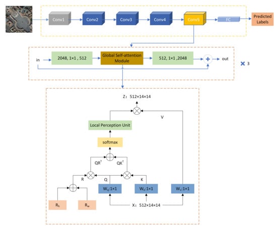
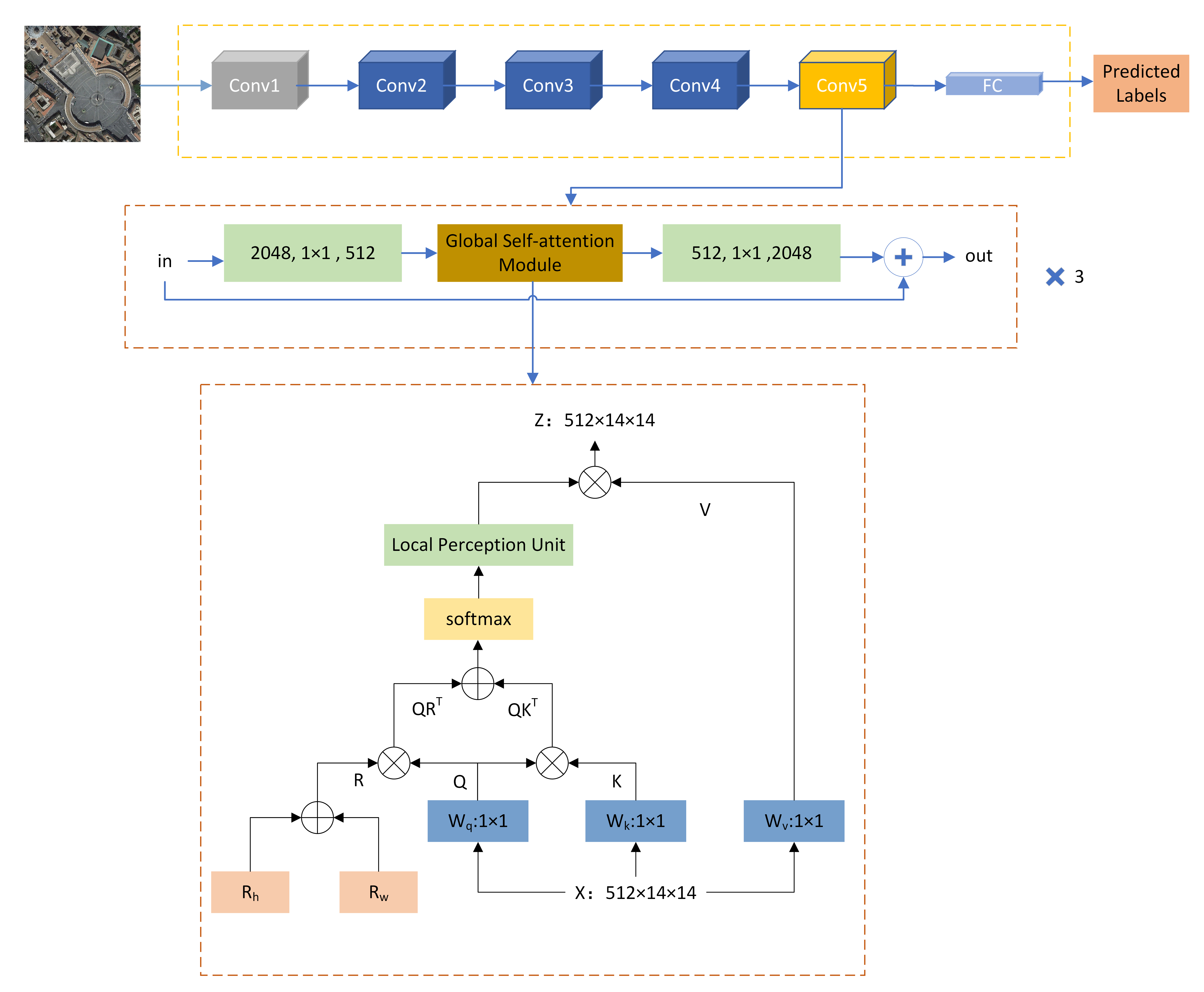
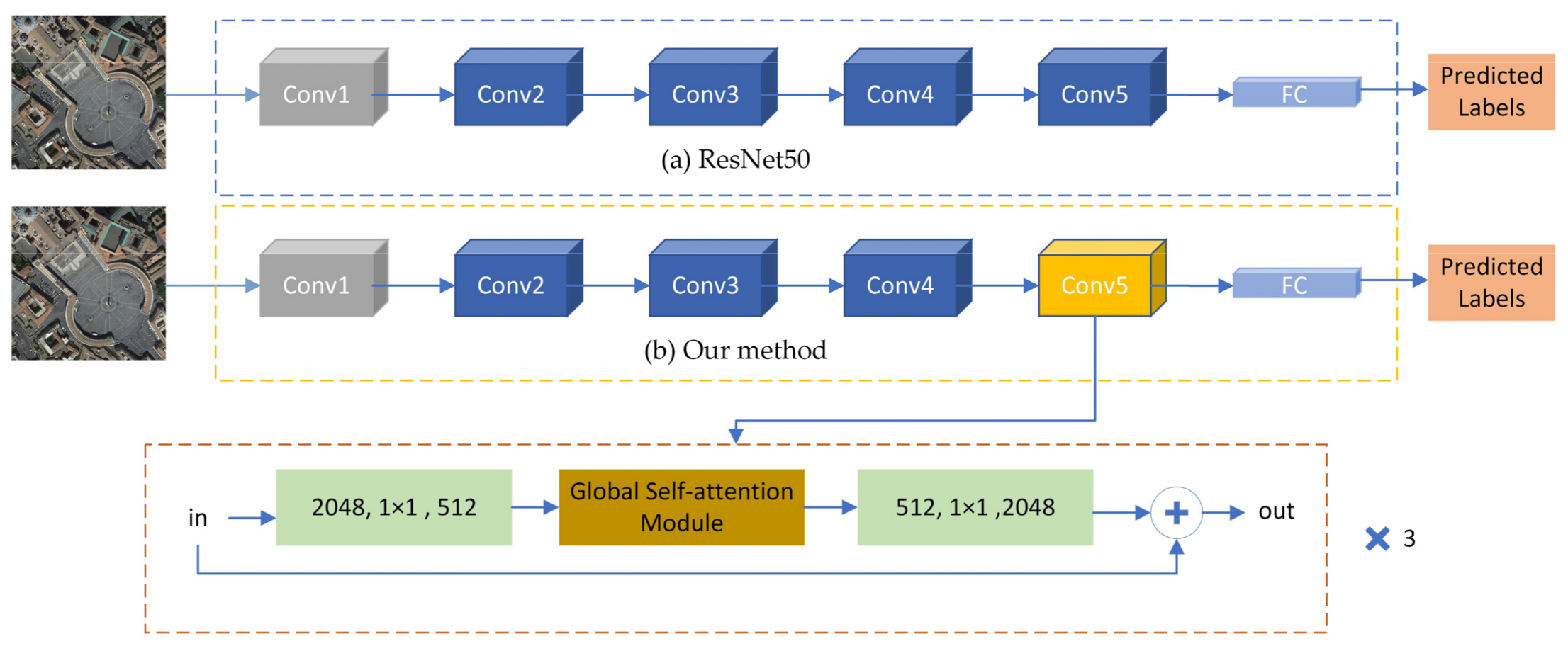
- We propose a network structure based on the global self-attention module and CNN. To address the problem of the inadequacy of CNN in extracting global information, the self-attention module is able to make the model have a global perceptual field by augmenting depth features on a global scale.
- (2)
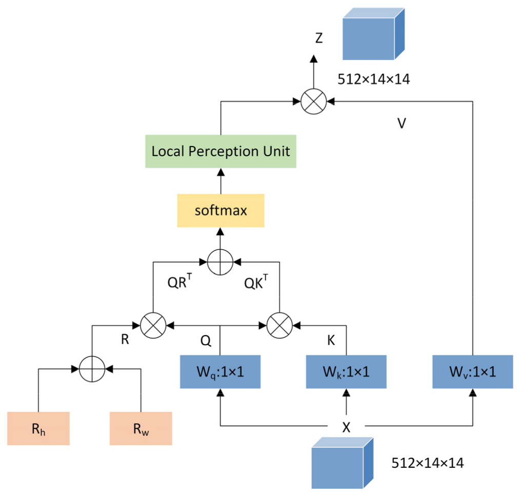
- The proposed global self-attention module can perceive the spatial location and local features of the image while enhancing global information.
- (3)
- With the purpose of optimizing the classification performance and mitigating the overfitting phenomenon, we use a data enhancement strategy. For the validity of our proposed model, extensive experiments were conducted and comparative analysis was carried out.
2. Materials and Methods
2.1. Overall Framework
| Algorithm 1: Our Method |
| Input: Training images |
| Output: Predicted labels of testing images |
| 1: Parameters initialization: initial learning ratio = 0.01, batch size = 16, the number of iterations = 80 |
| 2: Load parts of the parameters of the pre-trained ResNet50 model |
| 3: For iteration = 1:80 |
| For batch = 1:16 |
| Data preprocessing; |
| Calculate cross entropy loss; |
| Backpropagate loss; |
| Update model parameters |
| 4: The predicted labels of each testing image |
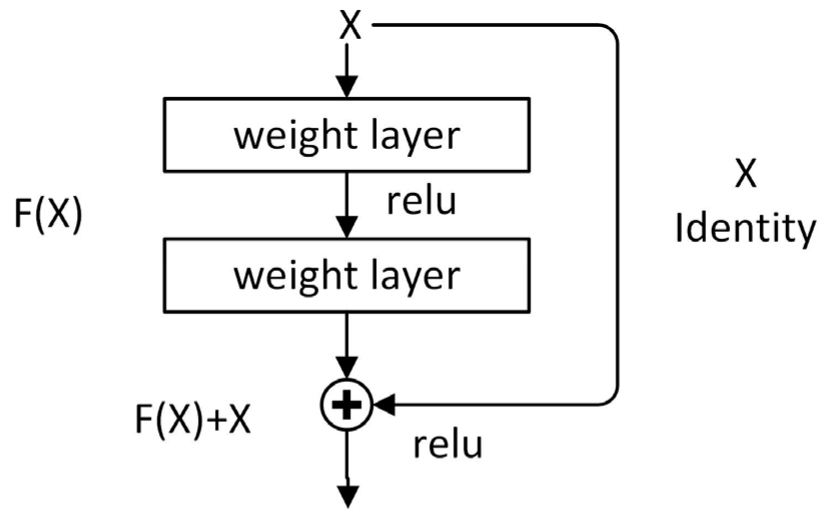
2.2. Basic Network
2.3. Global Self-Attention Module
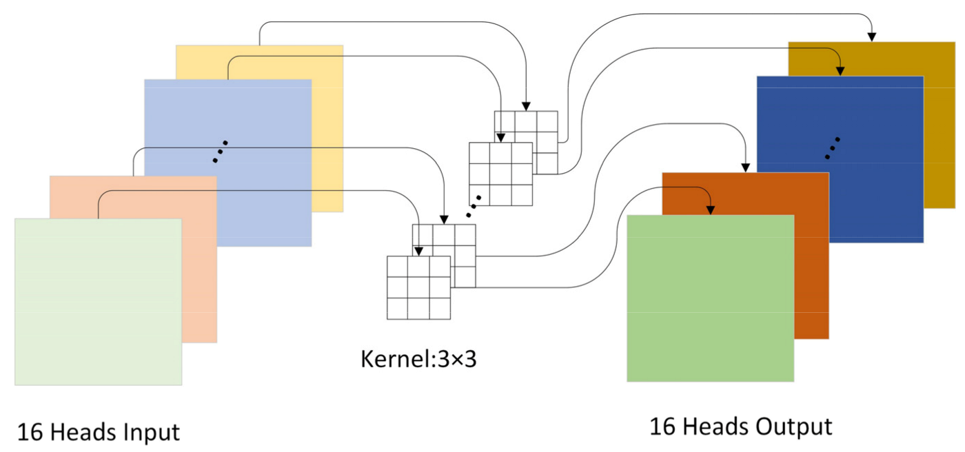
2.3.1. Multi-Head Self-Attention Layer
2.3.2. Relative Position Encoding
2.3.3. Local Perception Unit
2.4. Dataset Description
3. Experimental Results
3.1. Data Preprocessing
3.2. Experimental Setup and Evaluation Metrics
3.2.1. Experimental Setup
3.2.2. Evaluation Metrics
3.3. Accuracy Evaluation
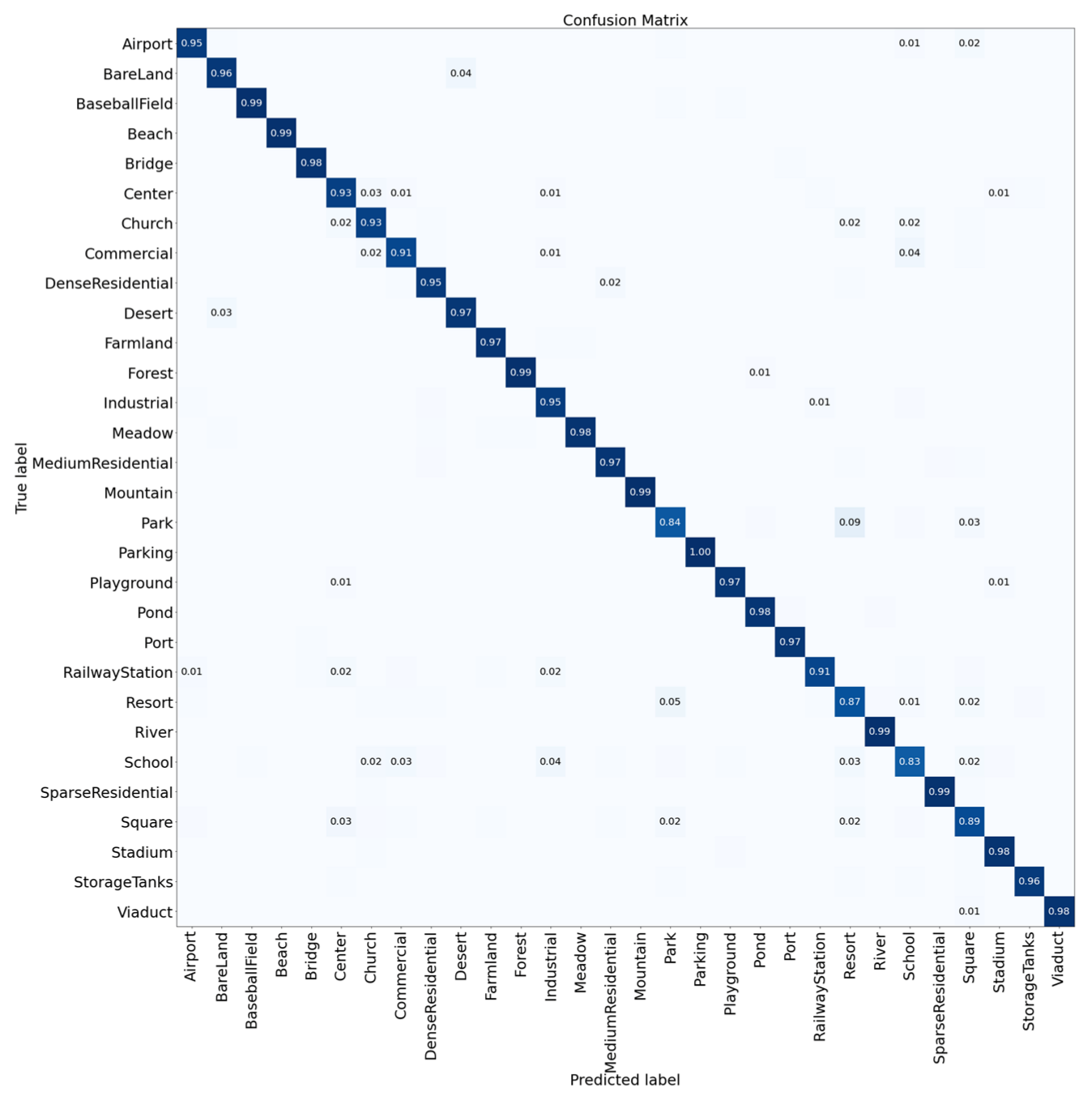
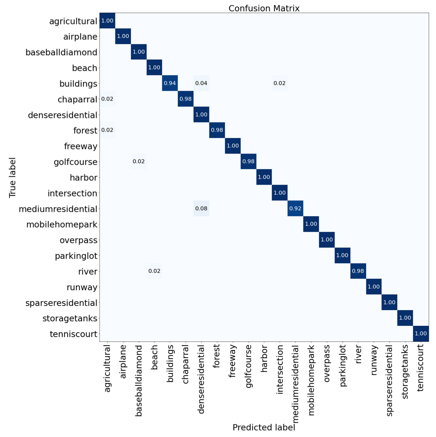
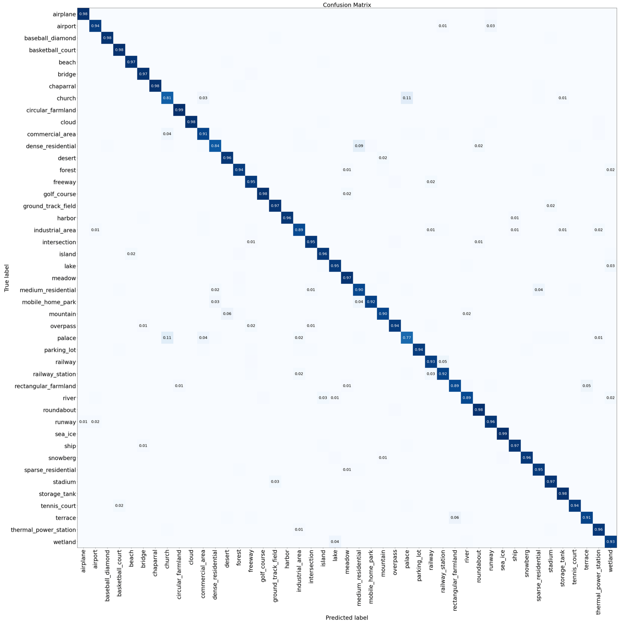
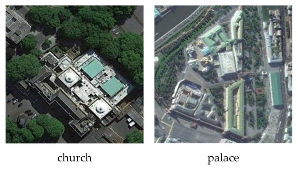
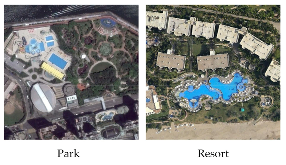
3.4. Confusion Matrix for Result Analysis
4. Discussion
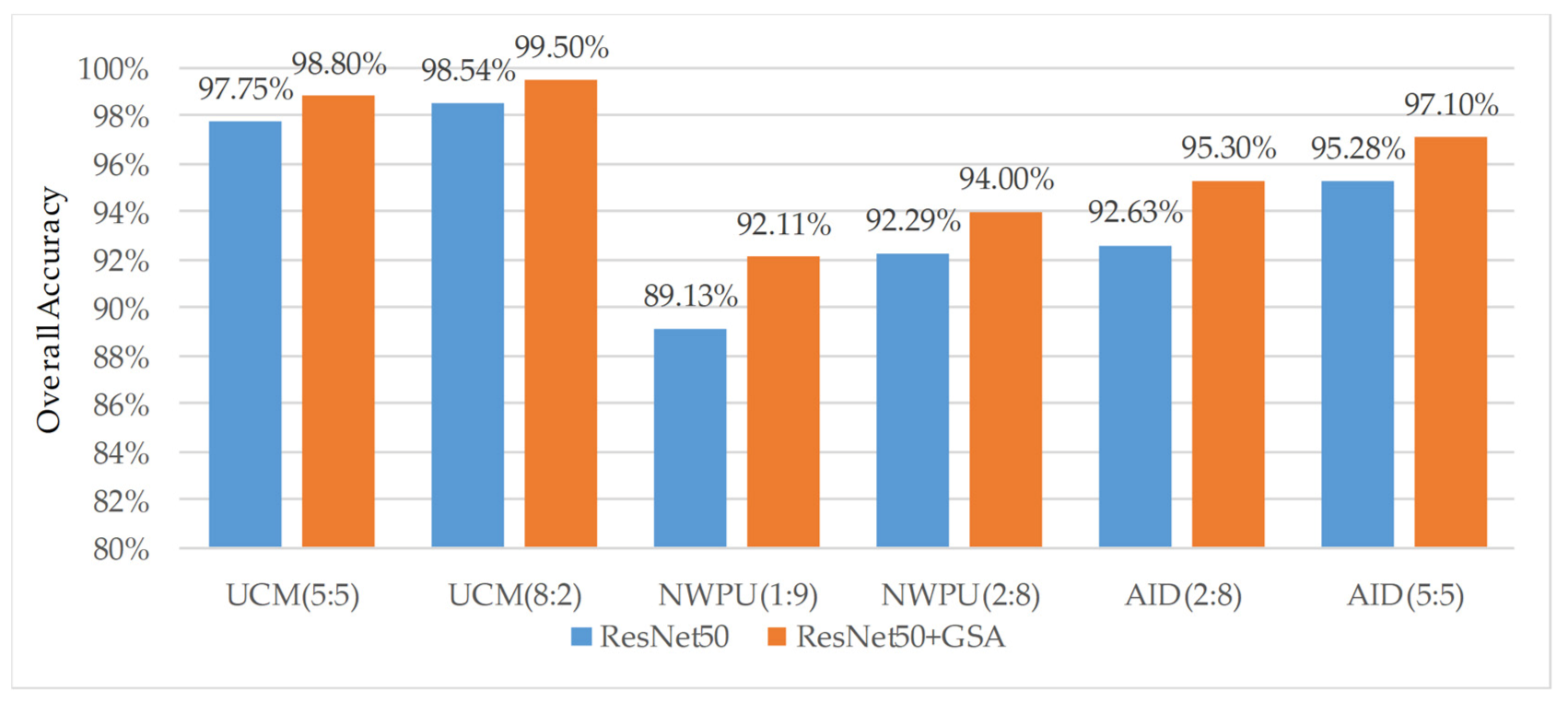
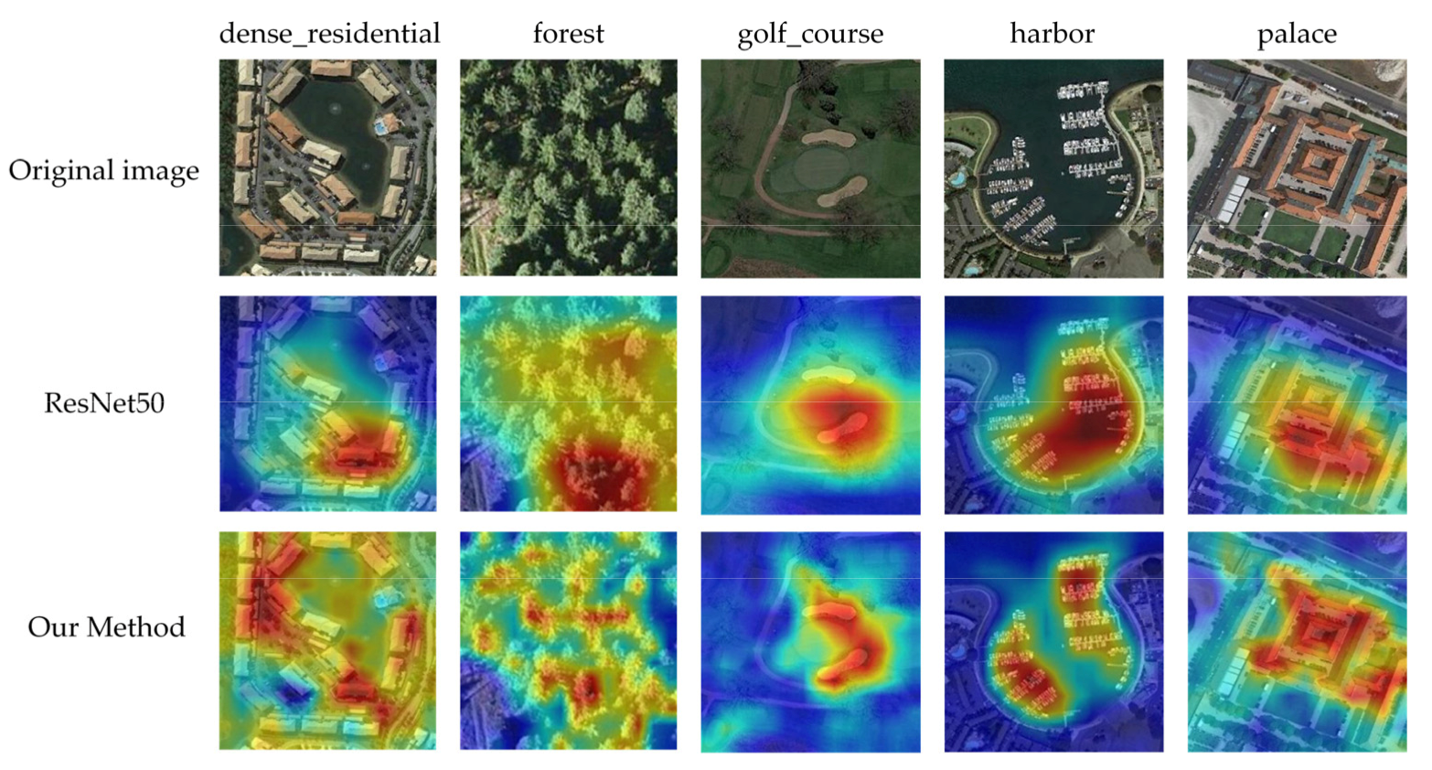
4.1. Analysis on the Improvement of Algorithm Accuracy by the Global Self-Attention Module
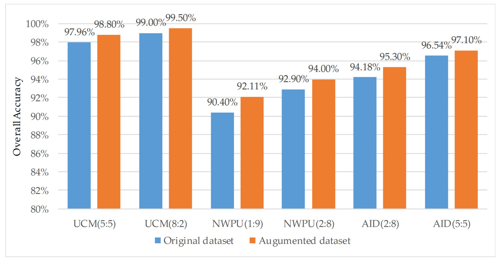
4.2. Analysis on the Improvement of Algorithm Accuracy by Data Augmentation
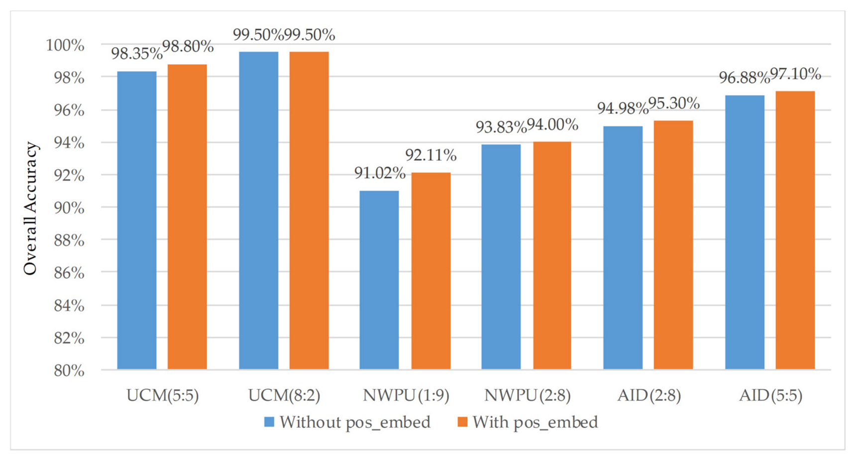
4.3. Analysis of the Improvement of Algorithm Accuracy by Relative Position Coding
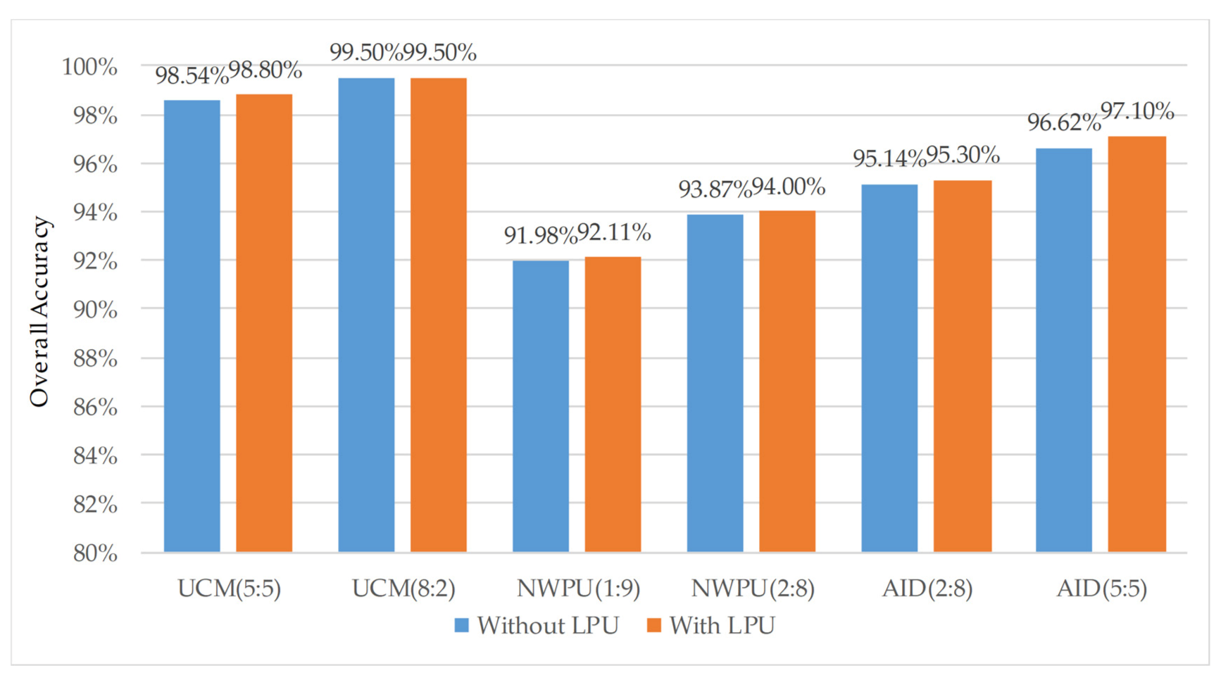
4.4. Analysis of the Improvement of Algorithm Accuracy by Local Perception Unit (LPU)
5. Conclusions
Author Contributions
Funding
Conflicts of Interest
Abbreviations
References
- Gómez-Chova, L.; Tuia, D.; Moser, G.; Camps-Valls, G. Multimodal Classification of Remote Sensing Images: A Review and Future Directions. Proc. IEEE 2015, 103, 1560–1584. [Google Scholar] [CrossRef]
- Longbotham, N.; Chaapel, C.; Bleiler, L.; Padwick, C.; Emery, W.; Pacifici, F. Very High Resolution Multiangle Urban Classification Analysis. IEEE Trans. Geosci. Remote Sens. 2011, 50, 1155–1170. [Google Scholar] [CrossRef]
- Zhang, T.; Huang, X. Monitoring of Urban Impervious Surfaces Using Time Series of High-Resolution Remote Sensing Images in Rapidly Urbanized Areas: A Case Study of Shenzhen. IEEE J. Sel. Top. Appl. Earth Obs. Remote Sens. 2018, 11, 2692–2708. [Google Scholar] [CrossRef]
- Cheng, G.; Han, J.; Zhou, P.; Guo, L. Multi-class geospatial object detection and geographic image classification based on collection of part detectors. ISPRS J. Photogramm. Remote Sens. 2014, 98, 119–132. [Google Scholar] [CrossRef]
- Ghaderpour, E.; Vujadinovic, T. Change Detection within Remotely Sensed Satellite Image Time Series via Spectral Analysis. Remote Sens. 2020, 12, 4001. [Google Scholar] [CrossRef]
- Panuju, D.R.; Paull, D.J.; Griffin, A.L. Change Detection Techniques Based on Multispectral Images for Investigating Land Cover Dynamics. Remote Sens. 2020, 12, 1781. [Google Scholar] [CrossRef]
- Fan, H. Feature Learning Based High Resolution Remote Sensing Image Scene Classification. Ph.D. Thesis, Wuhan University, Wuhan, China, 2017. [Google Scholar]
- Zhao, L.; Tang, P.; Huo, L.-Z. Land-Use Scene Classification Using a Concentric Circle-Structured Multiscale Bag-of-Visual-Words Model. IEEE J. Sel. Top. Appl. Earth Obs. Remote Sens. 2014, 7, 4620–4631. [Google Scholar] [CrossRef]
- Daniilidis, K.; Maragos, P.; Paragios, N. Improving the Fisher Kernel for Large-Scale Image Classification; Computer Vision—ECCV 2010; Lecture Notes in Computer Science; Springer: Berlin/Heidelberg, Germany, 2010; Volume 6314. [Google Scholar]
- Li, Q.; Qi, S.; Shen, Y.; Ni, D.; Zhang, H.; Wang, T. Multispectral Image Alignment with Nonlinear Scale-Invariant Keypoint and Enhanced Local Feature Matrix. IEEE Geosci. Remote Sens. Lett. 2015, 12, 1551–1555. [Google Scholar] [CrossRef]
- Ojala, T.; Pietikainen, M.; Maenpaa, T. Multiresolution gray-scale and rotation invariant texture classification with local binary patterns. IEEE Trans. Pattern Anal. Mach. Intell. 2002, 24, 971–987. [Google Scholar] [CrossRef]
- Dalal, N.; Triggs, B. Histograms of Oriented Gradients for Human Detection. In Proceedings of the IEEE Computer Society Conference on Computer Vision and Pattern Recognition (CVPR’05), San Diego, CA, USA, 20–25 June 2005. [Google Scholar] [CrossRef] [Green Version]
- Połap, D.; Włodarczyk-Sielicka, M.; Wawrzyniak, N. Automatic ship classification for a riverside monitoring system using a cascade of artificial intelligence techniques including penalties and rewards. ISA Trans. 2021. [Google Scholar] [CrossRef]
- Ma, L.; Liu, Y.; Zhang, X.; Ye, Y.; Yin, G.; Johnson, B.A. Deep learning in remote sensing applications: A meta-analysis and review. ISPRS J. Photogramm. Remote Sens. 2019, 152, 166–177. [Google Scholar] [CrossRef]
- Shin, H.-C.; Roth, H.R.; Gao, M.; Lu, L.; Xu, Z.; Nogues, I.; Yao, J.; Mollura, D.; Summers, R.M. Deep Convolutional Neural Networks for Computer-Aided Detection: CNN Architectures, Dataset Characteristics and Transfer Learning. IEEE Trans. Med Imaging 2016, 35, 1285–1298. [Google Scholar] [CrossRef] [Green Version]
- Hu, F.; Xia, G.-S.; Hu, J.; Zhang, L. Transferring Deep Convolutional Neural Networks for the Scene Classification of High-Resolution Remote Sensing Imagery. Remote Sens. 2015, 7, 14680–14707. [Google Scholar] [CrossRef] [Green Version]
- Zou, Q.; Ni, L.; Zhang, T.; Wang, Q. Deep Learning Based Feature Selection for Remote Sensing Scene Classification. IEEE Geosci. Remote Sens. Lett. 2015, 12, 2321–2325. [Google Scholar] [CrossRef]
- Dong, R.; Xu, D.; Jiao, L.; Zhao, J.; An, J. A Fast Deep Perception Network for Remote Sensing Scene Classification. Remote Sens. 2020, 12, 729. [Google Scholar] [CrossRef] [Green Version]
- Krizhevsky, A.; Sutskever, I.; Hinton, G.E. ImageNet classification with deep convolutional neural networks. Adv. Neural Inf. Process. Syst. 2012, 25, 1097–1105. [Google Scholar] [CrossRef]
- Simonyan, K.; Zisserman, A. Very deep convolutional networks for large-scale image recognition. In Proceedings of the 3rd International Conference on Learning Representations, San Diego, CA, USA, 7–9 May 2015; pp. 1–14. [Google Scholar] [CrossRef]
- Szegedy, C.; Liu, W.; Jia, Y.; Sermanet, P.; Reed, S.; Anguelov, D.; Erhan, D.; Vanhoucke, V.; Rabinovich, A. Going deeper with convolutions. In Proceedings of the IEEE Conference on Computer Vision and Pattern Recognition, Boston, MA, USA, 7–12 June 2015; pp. 1–9. [Google Scholar] [CrossRef] [Green Version]
- He, K.; Zhang, X.; Ren, S.; Sun, J. Deep residual learning for image recognition. In Proceedings of the IEEE Conference on Computer Vision and Pattern Recognition, Las Vegas, NV, USA, 27–30 June 2016; pp. 770–778. [Google Scholar] [CrossRef] [Green Version]
- Huang, G.; Liu, Z.; Van Der Maaten, L.; Weinberger, K.Q. Densely connected convolutional networks. In Proceedings of the IEEE Conference on Computer Vision and Pattern Recognition, Honolulu, HI, USA, 21–26 July 2017; pp. 2261–2269. [Google Scholar] [CrossRef] [Green Version]
- Chen, Z.; Wang, Y.; Han, W.; Feng, R.; Chen, J. An Improved Pretraining Strategy-Based Scene Classification With Deep Learning. IEEE Geosci. Remote Sens. Lett. 2019, 17, 844–848. [Google Scholar] [CrossRef]
- Shi, C.; Wang, T.; Wang, L. Branch Feature Fusion Convolution Network for Remote Sensing Scene Classification. IEEE J. Sel. Top. Appl. Earth Obs. Remote Sens. 2020, 13, 5194–5210. [Google Scholar] [CrossRef]
- Zhang, B.; Zhang, Y.; Wang, S. A Lightweight and Discriminative Model for Remote Sensing Scene Classification With Multidilation Pooling Module. IEEE J. Sel. Top. Appl. Earth Obs. Remote Sens. 2019, 12, 2636–2653. [Google Scholar] [CrossRef]
- Huang, H.; Xu, K. Combing Triple-Part Features of Convolutional Neural Networks for Scene Classification in Remote Sensing. Remote Sens. 2019, 11, 1687. [Google Scholar] [CrossRef] [Green Version]
- Ahonen, T.; Hadid, A.; Pietikäinen, M. Face Description with Local Binary Patterns: Application to Face Recognition. IEEE Trans. Pattern Anal. Mach. Intell. 2006, 28, 2037–2041. [Google Scholar] [CrossRef]
- Fang, J.; Yuan, Y.; Lu, X.; Feng, Y. Robust Space–Frequency Joint Representation for Remote Sensing Image Scene Classification. IEEE Trans. Geosci. Remote Sens. 2019, 57, 7492–7502. [Google Scholar] [CrossRef]
- Zhang, J.; Zhang, M.; Shi, L.; Yan, W.; Pan, B. A Multi-Scale Approach for Remote Sensing Scene Classification Based on Feature Maps Selection and Region Representation. Remote Sens. 2019, 11, 2504. [Google Scholar] [CrossRef] [Green Version]
- Yuan, Y.; Fang, J.; Lu, X.; Feng, Y. Remote Sensing Image Scene Classification Using Rearranged Local Features. IEEE Trans. Geosci. Remote Sens. 2018, 57, 1779–1792. [Google Scholar] [CrossRef]
- Li, E.; Xia, J.; Du, P.; Lin, C.; Samat, A. Integrating Multilayer Features of Convolutional Neural Networks for Remote Sensing Scene Classification. IEEE Trans. Geosci. Remote Sens. 2017, 55, 5653–5665. [Google Scholar] [CrossRef]
- Chaib, S.; Liu, H.; Gu, Y.; Yao, H. Deep Feature Fusion for VHR Remote Sensing Scene Classification. IEEE Trans. Geosci. Remote Sens. 2017, 55, 4775–4784. [Google Scholar] [CrossRef]
- Liang, J.; Deng, Y.; Zeng, D. A Deep Neural Network Combined CNN and GCN for Remote Sensing Scene Classification. IEEE J. Sel. Top. Appl. Earth Obs. Remote Sens. 2020, 13, 4325–4338. [Google Scholar] [CrossRef]
- Bi, Q.; Qin, K.; Zhang, H.; Li, Z.; Xu, K. RADC-Net: A residual attention based convolution network for aerial scene classification. Neurocomputing 2020, 377, 345–359. [Google Scholar] [CrossRef]
- Xu, R.; Tao, Y.; Lu, Z.; Zhong, Y. Attention-Mechanism-Containing Neural Networks for High-Resolution Remote Sensing Image Classification. Remote Sens. 2018, 10, 1602. [Google Scholar] [CrossRef] [Green Version]
- Chen, J.; Wang, C.; Ma, Z.; Chen, J.; He, D.; Ackland, S. Remote Sensing Scene Classification Based on Convolutional Neural Networks Pre-Trained Using Attention-Guided Sparse Filters. Remote Sens. 2018, 10, 290. [Google Scholar] [CrossRef] [Green Version]
- Kim, I.; Baek, W.; Kim, S. Spatially attentive output layer for image classification. In Proceedings of the IEEE/CVF Conference on Computer Vision and Pattern Recognition, Seattle, WA, USA, 14–19 June 2020; pp. 9533–9542. [Google Scholar]
- Shen, J.; Zhang, T.; Wang, Y.; Wang, R.; Wang, Q.; Qi, M. A Dual-Model Architecture with Grouping-Attention-Fusion for Remote Sensing Scene Classification. Remote Sens. 2021, 13, 433. [Google Scholar] [CrossRef]
- Li, J.; Lin, D.; Wang, Y.; Xu, G.; Zhang, Y.; Ding, C.; Zhou, Y. Deep Discriminative Representation Learning with Attention Map for Scene Classification. Remote Sens. 2020, 12, 1366. [Google Scholar] [CrossRef]
- Vaswani, A.; Shazeer, N.; Parmar, N.; Uszkoreit, J.; Jones, L.; Gomez, A.N.; Kaiser, Ł.; Polosukhin, I. Attention is all you need. Adv. Neural Inf. Process. Syst. 2017, 30, 5998–6008. [Google Scholar]
- Dosovitskiy, A.; Beyer, L.; Kolesnikov, A.; Weissenborn, D.; Zhai, X.; Unterthiner, T.; Dehghani, M.; Minderer, M.; Heigold, G.; Gelly, S.; et al. An image is worth 16 × 16 words: Transformers for image recognition at scale. arXiv 2020, arXiv:2010.11929. [Google Scholar]
- Devlin, J.; Chang, M.-W.; Lee, K.; Toutanova, K. BERT: Pre-training of deep bidirectional transformers for language under-standing. In Proceedings of the 2019 Conference of the North American Chapter of the Association for Computational Lin-guistics: Human Language Technologies, Minneapolis, MI, USA, 2–7 June 2019; Long and Short Papers. Volume 1, pp. 4171–4186. [Google Scholar]
- Wang, W.; Xie, E.; Li, X.; Fan, D.P.; Shao, L. Pyramid vision transformer: A versatile backbone for dense prediction without convolutions. arXiv 2021, arXiv:2102.12122. [Google Scholar]
- Wu, B.; Xu, C.; Dai, X.; Wan, A.; Zhang, P.; Tomizuka, M.; Keutzer, K.; Vajda, P. Visual transformers: Token-based image representation and processing for computer vision. arXiv 2020, arXiv:2006.03677. [Google Scholar]
- Bello, I.; Zoph, B.; Vaswani, A.; Shlens, J.; Le, Q.V. Attention Augmented Convolutional Networks. In Proceedings of the 2019 IEEE/CVF International Conference on Computer Vision (ICCV), Seoul, Korea, 27 October–2 November 2019; pp. 3285–3294. [Google Scholar]
- Srinivas, A.; Lin, T.-Y.; Parmar, N.; Shlens, J.; Abbeel, P.; Vaswani, A. Bottleneck Transformers for Visual Recognition. arXiv 2021, arXiv:2101.11605. [Google Scholar]
- Wu, H.; Zhao, S.; Li, L.; Lu, C.; Chen, W. Self-Attention Network With Joint Loss for Remote Sensing Image Scene Classification. IEEE Access 2020, 8, 210347–210359. [Google Scholar] [CrossRef]
- Shaw, P.; Uszkoreit, J.; Vaswani, A. Self-Attention with Relative Position Representations. arXiv Prepr. 2018, arXiv:1803.02155. [Google Scholar]
- Yang, Y.; Newsam, S. Bag-of-visual-words and spatial extensions for land-use classification. In Proceedings of the 18th SIGSPATIAL International Conference on Advances in Geographic Information Systems, San Jose, CA, USA, 3–5 November 2010; p. 270. [Google Scholar] [CrossRef]
- Cheng, G.; Han, J.; Lu, X. Remote Sensing Image Scene Classification: Benchmark and State of the Art. Proc. IEEE 2017, 105, 1865–1883. [Google Scholar] [CrossRef] [Green Version]
- Xia, G.-S.; Hu, J.; Hu, F.; Shi, B.; Bai, X.; Zhong, Y.; Zhang, L.; Lu, X. AID: A Benchmark Data Set for Performance Evaluation of Aerial Scene Classification. IEEE Trans. Geosci. Remote Sens. 2017, 55, 3965–3981. [Google Scholar] [CrossRef] [Green Version]
- Paszke, A.; Gross, S.; Massa, F.; Lerer, A.; Bradbury, J.; Chanan, G.; Killeen, T.; Lin, Z.; Gimelshein, N.; Antiga, L.; et al. PyTorch: An imperative style, high-performance deep learning library. In Advances in Neural Information Processing Systems; Curran Associates: Vancouver, BC, Canada, 2019; pp. 8024–8035. [Google Scholar]
- Xiong, W.; Lv, Y.; Cui, Y.; Zhang, X.; Gu, X. A Discriminative Feature Learning Approach for Remote Sensing Image Retrieval. Remote Sens. 2019, 11, 281. [Google Scholar] [CrossRef] [Green Version]
- Lv, Y.; Zhang, X.; Xiong, W.; Cui, Y.; Cai, M. An end-to end local-globalfusion feature extraction network for remote sensing image scene classification. Remote Sens. 2019, 11, 3006. [Google Scholar] [CrossRef] [Green Version]
- Liu, B.-D.; Meng, J.; Xie, W.-Y.; Shao, S.; Li, Y.; Wang, Y. Weighted Spatial Pyramid Matching Collaborative Representation for Remote-Sensing-Image Scene Classification. Remote Sens. 2019, 11, 518. [Google Scholar] [CrossRef] [Green Version]
- Liu, X.; Zhou, Y.; Zhao, J.; Yao, R.; Liu, B.; Zheng, Y. Siamese Convolutional Neural Networks for Remote Sensing Scene Classification. IEEE Geosci. Remote Sens. Lett. 2019, 16, 1200–1204. [Google Scholar] [CrossRef]
- He, N.; Fang, L.; Li, S.; Plaza, J.; Plaza, A. Skip-Connected Covariance Network for Remote Sensing Scene Classification. IEEE Trans. Neural Netw. Learn. Syst. 2019, 31, 1461–1474. [Google Scholar] [CrossRef] [Green Version]
- Shi, C.; Zhao, X.; Wang, L. A Multi-Branch Feature Fusion Strategy Based on an Attention Mechanism for Remote Sensing Image Scene Classification. Remote Sens. 2021, 13, 1950. [Google Scholar] [CrossRef]
- Zhao, Z.; Li, J.; Luo, Z.; Li, J.; Chen, C. Remote Sensing Image Scene Classification Based on an Enhanced Attention Module. IEEE Geosci. Remote Sens. Lett. 2020, 18, 1926–1930. [Google Scholar] [CrossRef]
- Fan, R.; Wang, L.; Feng, R.; Zhu, Y. Attention based Residual Network for High-Resolution Remote Sensing Imagery Scene Classification. In Proceedings of the 2019 IEEE International Geoscience and Remote Sensing Symposium, Yokohama, Japan, 28 July–2 August 2019. [Google Scholar]
- Tang, X.; Ma, Q.; Zhang, X.; Liu, F.; Ma, J.; Jiao, L. Attention Consistent Network for Remote Sensing Scene Classification. IEEE J. Sel. Top. Appl. Earth Obs. Remote Sens. 2021, 14, 2030–2045. [Google Scholar] [CrossRef]
- Guo, D.; Xia, Y.; Luo, X. Scene Classification of Remote Sensing Images Based on Saliency Dual Attention Residual Network. IEEE Access 2020, 8, 6344–6357. [Google Scholar] [CrossRef]
- Guo, Y.; Ji, J.; Lu, X.; Huo, H.; Fang, T.; Li, D. Global-Local Attention Network for Aerial Scene Classification. IEEE Access 2019, 7, 67200–67212. [Google Scholar] [CrossRef]
- Selvaraju, R.R.; Cogswell, M.; Das, A.; Vedantam, R.; Parikh, D.; Batra, D. Grad-CAM: Visual Explanations from Deep Net-works via Gradient-Based Localization. In Proceedings of the IEEE International Conference on Computer Vision; IEEE: Venice, Italy, 2017; pp. 618–626. [Google Scholar]


| Dataset | Number of Classes | Number of Images Per Class | Image Size | Resolution (m) | Year |
|---|---|---|---|---|---|
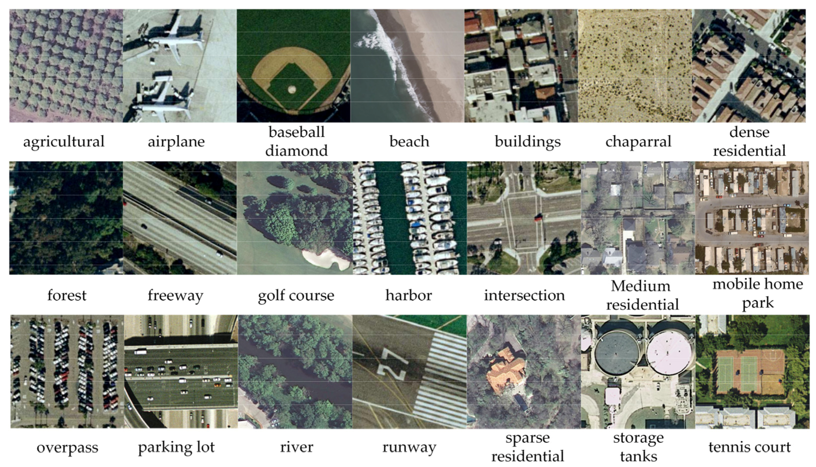
| UC Merced land-use dataset (UCM) | 21 | 100 | 256 * 256 | 0.3 | 2010 |
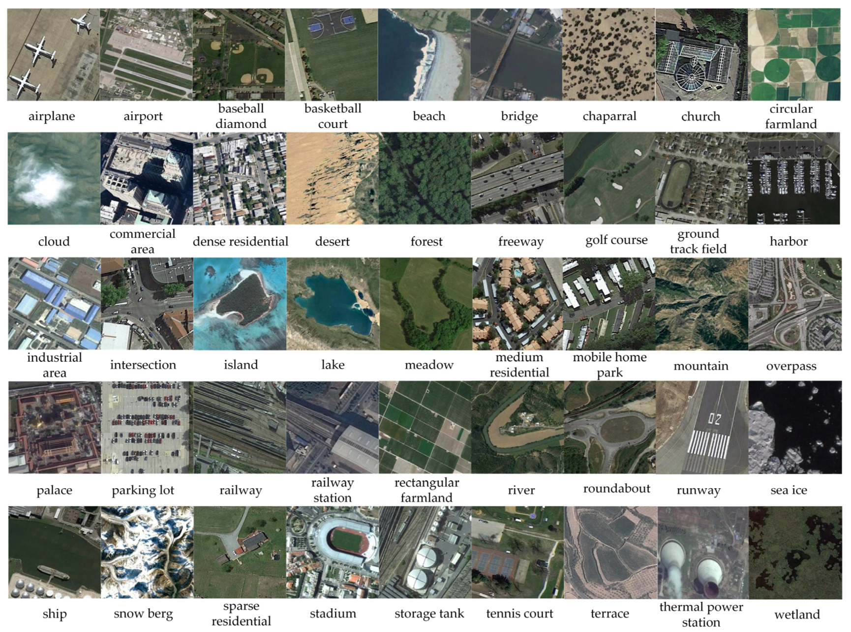
| NWPU-NESISC45 dataset (NWPU) | 45 | 700 | 256 * 256 | 0.2–30 | 2016 |
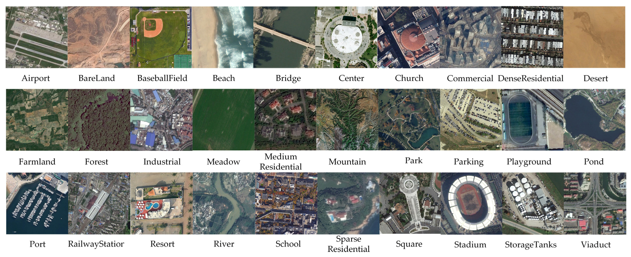
| Aerial Image Dataset (AID) | 30 | 220–420 | 600 * 600 | 0.5–8 | 2017 |
| Dataset | OA (%) | Kappa (%) | F1 |
|---|---|---|---|
| UCM (50%) | 98.80 | 98.75 | 98.82 |
| UCM (80%) | 99.50 | 99.21 | 99.25 |
| NWPU (10%) | 92.11 | 91.99 | 92.15 |
| NWPU (20%) | 94.00 | 93.87 | 94.04 |
| AID (20%) | 95.30 | 95.27 | 95.22 |
| AID (50%) | 97.10 | 97.06 | 97.05 |
| Methods | OA (50/50) (%) | OA (80/20) (%) |
|---|---|---|
| ResNet + weighted spatial pyramid matching collaborative representation based classification (WSPM-CRC) [56] | -- | 97.95 |
| Siamese ResNet_50 [57] | 90.95 | 94.29 |
| Skip-connected covariance (SCCov) [58] | -- | 99.05 ± 0.25 |
| Deep discriminative representation learning with attention map (DDRL-AM) [40] | -- | 99.05 ± 0.08 |
| Attention-oriented multi-branch CNN (AMB-CNN) [59] | -- | 99.52 ± 0.11 |
| ResNet-50+ attention-oriented multi-branch (EAM) [60] | -- | 98.98 ± 0.37 |
| Attention based Residual Network [61] | -- | 98.81 ± 0.30 |
| Attention consistent network (ACNet) [62] | -- | 99.76 ± 0.10 |
| Our Method | 98.80 ± 0.13 | 99.50 ± 0.08 |
| Methods | OA (10/90) (%) | OA (20/80) (%) |
|---|---|---|
| Saliency dual attention residualnetwork (SDAResNet) [63] | 89.40 | 91.15 |
| Siamese ResNet_50 [57] | -- | 92.28 |
| Global-local attention network (GLANet) [64] | 91.03 ± 0.18 | 93.45 ± 0.17 |
| SCCov [58] | 89.30 ± 0.35 | 92.10 ± 0.25 |
| DDRL-AM [40] | 92.17 ± 0.08 | 92.46 ± 0.09 |
| AMB-CNN [59] | 88.99 ± 0.14 | 92.42 ± 0.14 |
| ResNet-50+EAM [60] | 90.87 ± 0.15 | 93.51 ± 0.12 |
| Attention based Residual Network [61] | -- | 92.10 ± 0.30 |
| ACNet [62] | 91.09 ± 0.13 | 92.42 ± 0.16 |
| Our Method | 92.11 ± 0.06 | 94.00 ± 0.13 |
| Methods | OA (20/80) (%) | OA (50/50) (%) |
|---|---|---|
| GLANet [64] | 95.02 ± 0.28 | 96.66 ± 0.19 |
| SCCov [58] | 93.12 ± 0.25 | 96.10 ± 0.16 |
| DDRL-AM [40] | 92.36 ± 0.10 | -- |
| AMB-CNN [59] | 93.27 ± 0.22 | 95.54 ± 0.13 |
| ResNet-50+EAM [60] | 93.64 ± 0.25 | 96.62 ± 0.13 |
| ACNet [62] | 93.33 ± 0.29 | 95.38 ± 0.29 |
| Our Method | 95.30 ± 0.19 | 97.10 ± 0.23 |
Publisher’s Note: MDPI stays neutral with regard to jurisdictional claims in published maps and institutional affiliations. |
© 2021 by the authors. Licensee MDPI, Basel, Switzerland. This article is an open access article distributed under the terms and conditions of the Creative Commons Attribution (CC BY) license (https://creativecommons.org/licenses/by/4.0/).
Share and Cite
Li, Q.; Yan, D.; Wu, W. Remote Sensing Image Scene Classification Based on Global Self-Attention Module. Remote Sens. 2021, 13, 4542. https://doi.org/10.3390/rs13224542
Li Q, Yan D, Wu W. Remote Sensing Image Scene Classification Based on Global Self-Attention Module. Remote Sensing. 2021; 13(22):4542. https://doi.org/10.3390/rs13224542
Chicago/Turabian StyleLi, Qingwen, Dongmei Yan, and Wanrong Wu. 2021. "Remote Sensing Image Scene Classification Based on Global Self-Attention Module" Remote Sensing 13, no. 22: 4542. https://doi.org/10.3390/rs13224542
APA StyleLi, Q., Yan, D., & Wu, W. (2021). Remote Sensing Image Scene Classification Based on Global Self-Attention Module. Remote Sensing, 13(22), 4542. https://doi.org/10.3390/rs13224542